WO2018123559A1 - 情報処理装置、情報処理方法及びプログラム - Google Patents
情報処理装置、情報処理方法及びプログラム Download PDFInfo
- Publication number
- WO2018123559A1 WO2018123559A1 PCT/JP2017/044527 JP2017044527W WO2018123559A1 WO 2018123559 A1 WO2018123559 A1 WO 2018123559A1 JP 2017044527 W JP2017044527 W JP 2017044527W WO 2018123559 A1 WO2018123559 A1 WO 2018123559A1
- Authority
- WO
- WIPO (PCT)
- Prior art keywords
- elastic modulus
- external force
- distribution
- displacement amount
- information processing
- Prior art date
- Legal status (The legal status is an assumption and is not a legal conclusion. Google has not performed a legal analysis and makes no representation as to the accuracy of the status listed.)
- Ceased
Links
Images







Classifications
-
- A—HUMAN NECESSITIES
- A61—MEDICAL OR VETERINARY SCIENCE; HYGIENE
- A61B—DIAGNOSIS; SURGERY; IDENTIFICATION
- A61B5/00—Measuring for diagnostic purposes; Identification of persons
- A61B5/103—Measuring devices for testing the shape, pattern, colour, size or movement of the body or parts thereof, for diagnostic purposes
- A61B5/11—Measuring movement of the entire body or parts thereof, e.g. head or hand tremor or mobility of a limb
- A61B5/1104—Measuring movement of the entire body or parts thereof, e.g. head or hand tremor or mobility of a limb induced by stimuli or drugs
-
- A—HUMAN NECESSITIES
- A61—MEDICAL OR VETERINARY SCIENCE; HYGIENE
- A61B—DIAGNOSIS; SURGERY; IDENTIFICATION
- A61B1/00—Instruments for performing medical examinations of the interior of cavities or tubes of the body by visual or photographical inspection, e.g. endoscopes; Illuminating arrangements therefor
- A61B1/04—Instruments for performing medical examinations of the interior of cavities or tubes of the body by visual or photographical inspection, e.g. endoscopes; Illuminating arrangements therefor combined with photographic or television appliances
- A61B1/045—Control thereof
-
- A—HUMAN NECESSITIES
- A61—MEDICAL OR VETERINARY SCIENCE; HYGIENE
- A61B—DIAGNOSIS; SURGERY; IDENTIFICATION
- A61B5/00—Measuring for diagnostic purposes; Identification of persons
- A61B5/0059—Measuring for diagnostic purposes; Identification of persons using light, e.g. diagnosis by transillumination, diascopy, fluorescence
- A61B5/0077—Devices for viewing the surface of the body, e.g. camera, magnifying lens
-
- A—HUMAN NECESSITIES
- A61—MEDICAL OR VETERINARY SCIENCE; HYGIENE
- A61B—DIAGNOSIS; SURGERY; IDENTIFICATION
- A61B5/00—Measuring for diagnostic purposes; Identification of persons
- A61B5/103—Measuring devices for testing the shape, pattern, colour, size or movement of the body or parts thereof, for diagnostic purposes
- A61B5/11—Measuring movement of the entire body or parts thereof, e.g. head or hand tremor or mobility of a limb
- A61B5/1126—Measuring movement of the entire body or parts thereof, e.g. head or hand tremor or mobility of a limb using a particular sensing technique
- A61B5/1128—Measuring movement of the entire body or parts thereof, e.g. head or hand tremor or mobility of a limb using a particular sensing technique using image analysis
-
- A—HUMAN NECESSITIES
- A61—MEDICAL OR VETERINARY SCIENCE; HYGIENE
- A61B—DIAGNOSIS; SURGERY; IDENTIFICATION
- A61B8/00—Diagnosis using ultrasonic, sonic or infrasonic waves
- A61B8/08—Clinical applications
-
- G—PHYSICS
- G06—COMPUTING OR CALCULATING; COUNTING
- G06T—IMAGE DATA PROCESSING OR GENERATION, IN GENERAL
- G06T7/00—Image analysis
-
- G—PHYSICS
- G16—INFORMATION AND COMMUNICATION TECHNOLOGY [ICT] SPECIALLY ADAPTED FOR SPECIFIC APPLICATION FIELDS
- G16H—HEALTHCARE INFORMATICS, i.e. INFORMATION AND COMMUNICATION TECHNOLOGY [ICT] SPECIALLY ADAPTED FOR THE HANDLING OR PROCESSING OF MEDICAL OR HEALTHCARE DATA
- G16H30/00—ICT specially adapted for the handling or processing of medical images
- G16H30/40—ICT specially adapted for the handling or processing of medical images for processing medical images, e.g. editing
-
- G—PHYSICS
- G16—INFORMATION AND COMMUNICATION TECHNOLOGY [ICT] SPECIALLY ADAPTED FOR SPECIFIC APPLICATION FIELDS
- G16H—HEALTHCARE INFORMATICS, i.e. INFORMATION AND COMMUNICATION TECHNOLOGY [ICT] SPECIALLY ADAPTED FOR THE HANDLING OR PROCESSING OF MEDICAL OR HEALTHCARE DATA
- G16H50/00—ICT specially adapted for medical diagnosis, medical simulation or medical data mining; ICT specially adapted for detecting, monitoring or modelling epidemics or pandemics
- G16H50/50—ICT specially adapted for medical diagnosis, medical simulation or medical data mining; ICT specially adapted for detecting, monitoring or modelling epidemics or pandemics for simulation or modelling of medical disorders
Definitions
- the present invention relates to an information processing apparatus, an information processing method, and a program.
- Elastography techniques include, for example, nuclear magnetic resonance elasticity measurement (Magnetic Resonance Elastography: MRE) and ultrasonic elastography.
- MRE is an elastic modulus measurement method that uses magnetic resonance images (Magnetic Resonance Imaging: MRI), and is a method of imaging a measurement object that is vibrated from the outside and imaging a vibration wave that propagates within the target object.
- Magnetic Resonance Imaging Magnetic Resonance Imaging: MRI
- Ultrasonic elastography is a technique typified by a method of using a strain distribution of a tissue generated when an external pressure is applied to a measurement target, or a method of generating a shear wave in a target tissue and using its propagation velocity.
- the region range in which the elasticity information can be acquired by the elastography technique is limited to a local region where the wave propagates (surface portion of the target tissue) or a region near the region where pressure is applied.
- an object of the present invention is to provide a technique for estimating the elastic modulus distribution in the entire elastic body from local displacement information.
- the information processing apparatus includes an arithmetic unit that obtains the magnitude of an external force acting on a known action point and the elastic modulus distribution in the three-dimensional model.
- the invention according to claim 2 is the information processing apparatus according to claim 1, wherein the calculation unit obtains the magnitude of the external force and the distribution of the elastic modulus based on the following expression.
- E * is a set of E and f that minimizes the evaluation function J (E, f)
- E is an elastic modulus
- E 0 is a reference value of the elastic modulus
- f is The magnitude of the external force
- u 0 is the observed displacement
- L 0 (E) is the observable portion of the inverse matrix component of the overall stiffness matrix K expressed by the elastic modulus E
- L 0 ( E) f is an estimated displacement amount
- ⁇ is a coefficient
- 1 is a one-dimensional norm
- 2 is a two-dimensional norm.
- the invention according to claim 3 is an acquisition unit that acquires an observation displacement amount from an image obtained by imaging a part of an elastic body, a reception unit that receives an action point of an external force acting on the elastic body, and a three-dimensional structure of the elastic body.
- an estimation unit for estimating an estimated displacement amount of the three-dimensional model, and the observed displacement amount and the estimated displacement amount corresponding to the observed displacement amount includes an optimization unit that obtains the magnitude of the external force and the distribution of the elastic modulus in the three-dimensional model as an optimal solution for minimizing the difference.
- the invention according to claim 4 is the information processing apparatus according to claim 3, wherein the optimization unit obtains the magnitude of the external force and the distribution of the elastic modulus based on the following expression.
- E * is a set of E and f that minimizes the evaluation function J (E, f)
- E is an elastic modulus
- E 0 is a reference value of the elastic modulus
- f is The magnitude of the external force
- u 0 is the observed displacement
- L 0 (E) is the observable portion of the inverse matrix component of the overall stiffness matrix K expressed by the elastic modulus E
- L 0 ( E) f is an estimated displacement amount
- ⁇ is a coefficient
- 1 is a one-dimensional norm
- 2 is a two-dimensional norm.
- the invention according to claim 5 further includes an expression unit that expresses the three-dimensional model based on the distribution of the elastic modulus obtained as an optimal solution.
- a sixth aspect of the present invention is the information processing apparatus according to the first or third aspect, wherein the image is a still image captured by a single imaging camera.
- the invention according to claim 7 is characterized in that the optimum solution is obtained as a value that minimizes the sum of the absolute value sum of the change amount with respect to the initial value of the distribution of the elastic modulus and the difference.
- the invention according to claim 8 is characterized in that, when a plurality of pieces of information of the action points are given, the optimum solution is obtained as a value that minimizes the sum of the differences calculated for each of the action points.
- An information processing apparatus according to claim 1 or 3.
- the optimal solution is obtained as a value that minimizes the sum of the differences calculated for each of the external forces.
- the information processing apparatus according to claim 1 or 3, characterized in that A tenth aspect of the present invention is the information processing apparatus according to the first or third aspect, wherein there are a plurality of action points, and different external forces are applied to the action points.
- the invention according to claim 11 is the information processing apparatus according to claim 1 or 3, wherein the spatial resolution for obtaining the optimum solution is gradually increased from a low state.
- the invention according to claim 12 is characterized in that when the magnitude of the external force acting on the action point is given, the optimum solution is obtained as a distribution of the elastic modulus that minimizes the difference.
- Item 4. The information processing device according to Item 1 or 3.
- the invention according to claim 13 is a process for acquiring an observation displacement amount from an image obtained by imaging a part of an elastic body, a process for receiving an action point of an external force acting on the elastic body, and a three-dimensional model of the elastic body. Using the distribution of the elastic modulus and the magnitude of the external force as variables, the difference between the estimated displacement amount of the three-dimensional model and the estimated displacement amount corresponding to the observed displacement amount is minimized.
- the information processing method includes processing for obtaining the magnitude of the external force and the distribution of the elastic modulus in the three-dimensional model as an optimal solution to be converted.
- the invention according to claim 14 is a processing for acquiring an observation displacement amount from an image obtained by imaging a part of an elastic body, a process for receiving an action point of an external force acting on the elastic body, and a tertiary of the elastic body.
- the program executes a process for obtaining the magnitude of the external force and the distribution of the elastic modulus in the three-dimensional model.
- the elastic modulus distribution over the entire elastic body can be obtained.
- the distribution of the elastic modulus over the entire elastic body can be obtained.
- the elastic modulus distribution over the entire elastic body can be obtained.
- the elastic modulus distribution can be visually confirmed on the three-dimensional model.
- the apparatus structure used for observation of an elastic body can be simplified.
- the tenth aspect of the present invention it is possible to improve the estimation accuracy as compared with the case where only one action point and one external force are used for obtaining the displacement amount.
- a highly accurate estimation result can be obtained with the passage of time.
- the estimation accuracy can be increased as compared with the case where the magnitude of the external force is not given.
- the thirteenth aspect of the present invention even when the region where the amount of displacement can be acquired is limited to a part of the elastic body, the distribution of the elastic modulus over the entire elastic body can be obtained.
- the fourteenth aspect of the present invention even when the region where the amount of displacement can be acquired is limited to a part of the elastic body, the distribution of the elastic modulus over the entire elastic body can be obtained.
- FIG. 10 is a diagram for explaining observation conditions used in the second embodiment. It is a figure which shows the experimental result in the case where the pattern used for estimation of distribution of the elasticity modulus E is 1 set (Embodiment 1), and the pattern is 2 sets (Embodiment 2).
- FIG. 10 is a diagram for explaining the relationship between the ratio of the number of observed vertices and the observation accuracy in the case of the third embodiment.
- FIG. 1 is a diagram for explaining a conceptual image of an estimation method employed in an embodiment described later. As shown in FIG. 1, each embodiment assumes that the entire elastic body 1 cannot be observed (that is, a portion that can be observed and a portion that cannot be observed), and a portion that can be observed in each embodiment.
- This paper describes a method for estimating the elastic modulus distribution in the entire elastic body using local displacement information.
- the estimation process is executed using the fact that the position information of the acting point Pa of the external force F that deforms the elastic body 1 is known.
- the position information of the action point Pa may be given to the processing system before the estimation process starts, and the position of the action point Pa is arbitrary. Therefore, as shown in FIG. 1, it is not necessary to be present in a portion where the position of the action point Pa can be observed.
- the information that gives the magnitude f of the external force F acting on the action point Pa and the position information of the part (fixed point) Pf where the elastic body 1 is fixed around are known or unknown. good. In general, the more information that is known, the higher the estimation accuracy and the less the calculation time required for estimation.
- FIG. 1 for explaining the observable portion and the unobservable portion, a state in which a part of the elastic body 1 is covered with the shielding object 2 is illustrated, but a part of the elastic body 1 is covered with the shielding object 2. It is not essential to be.
- a portion included in the observation visual field is a portion that can be observed, and a portion not included in the observation visual field is a portion that cannot be observed. Therefore, the portion (for example, the back side or the back side) that is behind the elastic body 1 when viewed from the observation direction is an example of a portion that cannot be observed.
- the displacement amount of the part which can be observed among the elastic bodies 1 shall be pinpointed for every site
- the displacement amount may be given only for the surface region of the elastic body 1 or may be given including the internal region of the elastic body 1. In general, the more the region where the amount of displacement is specified (the more the proportion of the portion that can be observed increases), the higher the accuracy of estimating the elastic modulus.
- the elastic modulus in each embodiment includes a Young's modulus E representing hardness in the indentation / tensile direction, a rigidity modulus G representing hardness in the shearing direction, a Poisson's ratio ⁇ , a bulk modulus K, and the like.
- the elastic modulus is used as the Young's modulus.
- the elastic body 1 refers to a substance having a property of returning to the original dimensions when the action of the external force F is stopped while the distortion is generated (deformed) by the action of the external force F.
- an elastic body that is approximately expressed by using Hooke's law such as various organs in a living tissue, is assumed.
- the elastic modulus distribution in the elastic body 1 is not uniform.
- the case where the elastic modulus distribution is not uniform means, for example, that the elastic modulus of at least a part of the elastic body 1 is different from the surrounding elastic modulus.
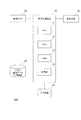
- FIG. 2 is a diagram illustrating a hardware configuration example of the information processing system 100.
- the information processing system 100 includes an information processing apparatus 10 that performs arithmetic processing for estimating the elastic modulus distribution of the elastic body 1 (see FIG. 1), at least one imaging camera 20 that is used to image the elastic body 1, and an elastic body.
- a user operates a three-dimensional image data storage device 30 that stores three-dimensional image data (volume data) used to create one mesh model, a display device 40 that is used to display an estimated elastic modulus distribution, and the like.
- an input device 50 including a mouse and a pointing device.
- the information processing apparatus 10 is a so-called computer, and includes a CPU (Central Processing Unit) 11 that executes a program, a ROM (Read Only Memory) 12 that stores programs and data such as BIOS (Basic Input / Output System) and firmware.
- a RAM (Random Access Memory) 13 that gives a work area to the program and a storage unit 14 that stores image data to be processed.
- the storage unit 14 is a storage device such as a hard disk device or a semiconductor memory. Functions realized through execution of the program by the CPU 11 will be described later.
- the imaging camera 20 is an imaging device used for observing the elastic body 1.
- the imaging camera 20 may be an imaging device suitable for observing the elastic body 1.
- an infrared camera, an endoscopic camera, an ultrasonic imaging apparatus, an optical ultrasonic imaging apparatus, or the like is used as the imaging camera 20.
- the information processing apparatus 10 can specify the amount of displacement of each part through movement of feature points and infrared markers existing on the surface of the elastic body 1.
- the ultrasonic imaging apparatus is used, the information processing apparatus 10 can specify the displacement amount of each part including the inside of the elastic body 1.
- the imaging device of the endoscope camera may be a CCD (Charge Coupled Device) or a CMOS (Complementary MOS).
- a single imaging camera 20 is used, and a still image obtained by photographing the elastic body 1 from one direction is output.
- the three-dimensional image data storage device 30 is a large-capacity hard disk device that stores, as three-dimensional image data, images (reconstructed images) reconstructed so that tomographic image data acquired by tomographic imaging of the elastic body 1 is stacked. Consists of.
- the three-dimensional image data storage device 30 may exist as a server or network storage on the network as well as when directly connected to the information processing device 10.
- CT Computed Tomography
- PET Positron Emission Tomography
- MRI Magnetic resonance imaging
- the display device 40 is composed of a liquid crystal display, for example.
- the liquid crystal display includes a liquid crystal panel, a backlight, and the like.
- the display device 40 may be an organic EL (ElectroLuminescence) display or the like.
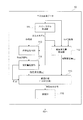
- FIG. 3 is a diagram illustrating an example of a functional configuration realized through execution of a computer program by the CPU 11.
- the information processing apparatus 10 includes a mesh model generation unit 111 that generates a three-dimensional mesh model, and a displacement amount (observation displacement amount u o) about an observation site from a camera image output from the imaging camera 20. ), An action point receiving unit 113 that receives position information of the action point Pa, and a displacement amount (estimated displacement amount u at each part of the mesh model by applying the action point information to the mesh model.
- the mesh model generation unit 111 takes in the three-dimensional image data of the elastic body 1 to be observed from the three-dimensional image data storage device 30, the mesh model generation unit 111 is a collection of simple shape elements from the three-dimensional image data given as a continuum. This is a functional unit that generates a certain mesh model.
- the mesh model here is an example of a three-dimensional model, and the minimum element is represented by a cube or tetrahedron (triangular pyramid).
- FIG. 4 is a diagram showing an example of a mesh model 200 in which the elastic body 1 is expressed by a mesh structure.
- FIG. 4 shows the mesh model 200 before the external force F (see FIG. 5) is applied to the action point Pa (see FIG. 5).
- a circle in the figure indicates a node of the minimum element.
- FIG. 5 shows the mesh model 200 after being elastically deformed by applying an external force F with the lower right end of the mesh model 200 as an action point Pa.
- the observation displacement amount acquisition unit 112 compares the camera image before the external force F is applied to the action point Pa with the camera image after the external force F is applied to the action point Pa, and observes the displacement of each part appearing in the image. It is a functional unit that acquires the quantity u o .
- the observation displacement amount u o acquired by the observation displacement amount acquisition unit 112 is a displacement amount for each position specified on the camera image, and the positional relationship with the voxels constituting the mesh model 200 is unknown. .
- the observation displacement amount acquisition unit 112 has a processing function for matching the three-dimensional image data or the mesh model 200 (see FIG. 4) with the camera image and associating the observation displacement amount u o with each vertex of the mesh model 200. Has been. At the time of the association here, processing for aligning the dimensions of the 3D image data or mesh model 200 and the dimensions of the camera image is also executed.
- the more image information included in the three-dimensional image data or the mesh model 200 the higher the matching accuracy with the camera image.
- the mesh model 200 is used for matching, if the rendering image obtained by rendering the surface information of the three-dimensional image data on the surface of the mesh model 200 is compared with the luminance information of the camera image, the vertex of the mesh model 200 is matched with high accuracy. observed displacement u o can be associated.
- the action point receiving unit 113 is a functional unit that receives position information of the action point Pa through the input device 50. For example, when a click operation is detected, the action point receiving unit 113 receives the part on the mesh model 200 where the mouse cursor is located as the action point Pa of the external force F. The action point accepting unit 113 specifies the position of the accepted action point Pa by the identification number of the vertex on the mesh model 200 and outputs it to the displacement amount estimating unit 114.
- the distribution of the elastic modulus E of the elastic body 1 and the magnitude f (vector) of the external force F applied to the elastic body 1 are final estimation targets. Since the elastic modulus E is an inclusion parameter of the overall stiffness matrix K, if the overall stiffness matrix K is specified, the elastic modulus E is also specified.
- FIG. 6 is a two-dimensional mesh model.
- the information processing system 100 handles a three-dimensional mesh model 200.
- the triangular element I is defined by vertex numbers 1, 2 and 3
- the triangular element II is defined by vertex numbers 2, 3 and 4.
- the element stiffness matrix K e to be used is derived from the following Equation 3.
- V is the volume of the triangular element.
- the B matrix is a matrix obtained from the shape function of the element, and the D matrix is a matrix obtained from the elastic modulus E and the Poisson's ratio ⁇ .
- the D matrix can be expressed by the following formula (Formula 4). As can be seen from Equation 4, the D matrix is a function of the elastic modulus E. Therefore, the element stiffness matrix K e is also expressed as a function of the elastic modulus E.
- Overall stiffness matrix K is an element stiffness matrix K e elements I triangle is given by the sum of the element stiffness matrix K e elements II triangular. That is, the overall stiffness matrix K is an element stiffness matrix K e elements I triangle composed of vertex number 1, 2, 3, element stiffness matrix elements II triangular composed of vertex number 2, 3, 4 Expressed as the sum of Ke.
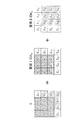
- FIG. 7 is a diagram explaining the concept of processing overlay element stiffness matrix K e.
- FIG. 7 shows that the overall stiffness matrix K is represented by the sum of the element stiffness matrix K e of the element I and the element stiffness matrix K e of the element II.
- the element stiffness matrix K e is a function of the elastic modulus E
- the overall stiffness matrix K expressed by the sum is also a function of the elastic modulus E. Therefore, the overall stiffness matrix K in the mesh model 200 in the present embodiment is also a function of the elastic modulus E.
- the camera image of the present embodiment is an image obtained by capturing a part of the elastic body 1 that has been elastically deformed by the external force F whose known point of action Pa is known but whose magnitude f is unknown. Therefore, the unknown parameters in Equation 2 are the elastic modulus E distribution (overall stiffness matrix K) and the magnitude f (vector) of the external force F.
- the displacement amount estimation unit 114 sets an arbitrary value for each of these unknown parameters and calculates the estimated displacement amount u o ′.
- the displacement amount estimation unit 114 gives initial values to the distribution of the elastic modulus E (overall stiffness matrix K) and the magnitude f of the external force F, which are unknown parameters.
- the estimated displacement u o ′ is calculated.
- Expression 2 When Expression 2 is expressed as a matrix, the following expression (Expression 5) is obtained.
- u o ′ is an estimated displacement amount of a portion that can be observed
- u i ′ is an estimated displacement amount of a portion that cannot be observed.
- L o is a moiety that can be observed among the inverse matrix component of the overall stiffness matrix K expressed by the elastic modulus E
- L i can not be observed among the inverse matrix component of the overall stiffness matrix K expressed in modulus of elasticity E Part.
- f o is the magnitude of the external force F acting on the vertex of the portion that can be observed
- f i is the magnitude of the external force F acting on the vertex of the portion that cannot be observed.
- Expression 5 Focusing on the estimated displacement u o ′ of the portion that can be observed, Expression 5 can be expressed as the following Expression (Expression 6).
- Expression 6 since the action point Pa is known, the magnitude of the external force F corresponding to a vertex other than the action point Pa among the magnitude f of the external force F can be represented by 0 (zero).
- the displacement amount estimation unit 114 calculates an estimated displacement amount u o ′ (including an initial value) based on the component L o represented by the elastic modulus E and the magnitude f of the external force F using Expression 6.
- the optimization unit 115 estimates the estimated displacement amount u o ′ for all vertex numbers (including not only the observable portion but also the observable portion vertex) of the mesh model 200, and the partial image captured by the imaging camera 20.
- the combination of unknown parameters is updated until an overall stiffness matrix K (that is, a distribution of elastic modulus E) and an external force f that minimize the difference from the observation displacement amount u o specified from the above are obtained.
- the optimization unit 115 performs an optimization problem for obtaining an unknown parameter that minimizes the difference between the estimated displacement amount u o ′ and the observed displacement amount u o (that is, gives the deformation closest to the observation result). Execute the solving process.
- This processing is expressed by the following formula (Formula 7).
- E * means a set of E and f that minimizes the evaluation function J (E, f).
- the evaluation function J (E, f) is given by the L 2 norm of the difference between the estimated displacement amount u o ′ and the observed displacement amount u o .
- the optimization unit 115 updates the unknown parameters E and f until the minimum value of the evaluation function J is obtained, and feeds back the updated values to the displacement amount estimation unit 114. That is, the recalculation of the estimated displacement u o ′ by the displacement estimator 114 using the updated values of the unknown parameters E and f and the evaluation of the estimated displacement u o ′ by the optimizer 115 are as follows. It is repeatedly executed until the minimum value is obtained.
- a Covariance Matrix Adaptation Evolution Strategy (CMA-ES) is used as a technique for solving the optimization problem.
- CMA-ES Covariance Matrix Adaptation Evolution Strategy
- other known methods may be used as a method for solving the optimization problem. For example, a gradient method, a Monte Carlo method, an annealing method, or the like may be used.
- the displacement amount estimation unit 114 and the optimization unit 115 are drawn as separate functional units, but may be included in one functional unit.
- the expression unit 116 displays an image representing the distribution of the elastic modulus E identified as the optimum solution and the distribution of the elastic modulus E out of the magnitude of the external force F superimposed on the mesh model 200 on the display device 40 ( (See FIG. 2).
- the expression unit 116 expresses the difference in elastic modulus E as a difference in color and brightness.
- the expression unit 116 may display the numerical value of the elastic modulus E corresponding to each part of the mesh model 200. It should be noted that the expression unit 116 outputs the magnitude f of the external force F obtained as an optimal solution as necessary.
- the method according to the embodiment is described as a program using Visual C / C ++, and the created program is executed on a general-purpose computer (OS: Windows 10 Pro, CPU: IntelCorei7-6700K, memory: 16 GB) did.
- OS Windows 10 Pro
- CPU IntelCorei7-6700K
- memory 16 GB
- the simulation was performed on a rectangular parallelepiped mesh model 200 (see FIG. 5).
- This mesh model 200 has 99 vertices in total, and the minimum element is a tetrahedron.
- the nine vertices located at the left end of the mesh model 200 are fixed ends Pf, and the other points are free points. Furthermore, as shown in FIG. 5, three vertices located at the lower right end of the mesh model 200 are designated as the action points Pa of the external force F. It is assumed that the external force F having the same magnitude f acts downward ( ⁇ z-axis direction) on these three vertices.
- FIG. 8 is a diagram in which the distribution of the elastic modulus E used as a true value is superimposed on the mesh model 200.
- the elastic modulus E used as a true value is superimposed on the mesh model 200.
- the elastic modulus E is large (hard), and the elastic modulus E of the other part takes the same value.
- white circle nodes represent positions that can be observed, and black circle nodes represent positions that cannot be observed.
- the elastic modulus E of the four cubic blocks located in the seventh and eighth left columns from the right end of the 40 cubic blocks to the left ( ⁇ x direction) is 2.0. [MPa] is hard and the elastic modulus E of the other part is 1.0 [MPa].
- the distribution of the elastic modulus E of all the vertices of the mesh model 200 is estimated based on the camera image observed when the external force F is applied to the mesh model 200 shown in FIG. did.
- the mesh model 200 shown in FIG. 8 applies an external force F of 10 N downward ( ⁇ z-axis direction) to the three apexes at the lower right end of the mesh model 200 of the elastic body 1 as in the description of FIG. This represents a deformed state.
- the magnitude f of the external force F is also an unknown parameter.
- FIG. 9 is a diagram for explaining the ratio of the number of vertices that can be observed in the mesh model 200.
- FIG. 9 is a diagram in which the mesh model 200 is observed from the lateral direction (xz plane), and is divided into 10 subsections in the x-axis direction.
- the case where one small section is observed corresponds to the case where 10% of the whole is observed, and the case where two small sections are observed corresponds to the case where 20% of the whole is observed. Similarly, the case where nine subsections are observed corresponds to the case where 90% of the whole is observed.
- the estimation accuracy of the elastic modulus E is expected to be affected by the number of dimensions of the estimation space.
- the number of dimensions of the estimated space is expressed by the estimated resolution of the elastic modulus E.
- a low number of dimensions in the estimation space means that the estimation is performed at a low resolution
- a high number of dimensions means that the estimation is performed at a high resolution.
- the number of dimensions of the estimated space represents how many unit sections (blocks) each mesh model 200 is divided into.
- FIG. 10 is a diagram for explaining the relationship between the estimated number of blocks N and the size of a unit block (block) from which the elastic modulus E is estimated.
- the larger the value of the estimated number of blocks N the smaller the estimated size of the unit section), the higher the spatial resolution, and the higher the resolution of the elastic modulus E can be estimated.
- FIG. 11 is a diagram illustrating experimental results when the estimated number of blocks N is 10, 20 is 40, and 40 is.
- the vertical axis in FIG. 11 represents the mean square error (Root Mean Square Error: RMSE) between the true elastic modulus E and the estimated elastic modulus E ′, and the horizontal axis represents the ratio of the total number of observable vertices (FIG. 9). Reference).
- RMSE Root Mean Square Error
- the elastic modulus E when the mesh model 200 is expressed by 10 blocks (when estimated at a low resolution), even if the number of observable vertices is about 15% of the entire mesh model 200, the elastic modulus E is highly accurate. It can be seen that can be estimated. In this case, the calculation cost is low because the number of blocks is small. Further, when the mesh model 200 is expressed by 20 blocks (when estimated at medium resolution), the elastic modulus E can be estimated with high accuracy when the number of observable vertices is about 50% of the entire mesh model 200. I understand. When expressing the mesh model 200 with 40 blocks (when estimating with high resolution), the least square error must not be sufficiently reduced unless the number of observable vertices is about 70% of the entire mesh model 200. I understand.
- the low resolution, medium resolution, and high resolution are merely representations of the relative relationship between the three resolutions.
- the observed displacement u o acquired from an image obtained by imaging a part (for example, 50% of the whole) of the elastic body 1 and the estimated displacement calculated for the mesh model 200 of the elastic body 1
- the magnitude f of the external force F acting on the known action point Pa and by obtaining the distribution of the elastic modulus E in the mesh model 200 throughout the region can be acquired observation displacement u o Find the distribution of the elastic modulus E of the elastic member 1 whole even if limited to a portion of the elastic body 1 Can do.
- the estimation accuracy depends on the resolution of the estimated space and the ratio of observable vertices. If it is desired to estimate the elastic modulus E of the elastic body 1 with high resolution, the area of the elastic body 1 imaged by the imaging camera 20 is estimated. When it is desired to estimate the elastic modulus E of the elastic body 1 with low resolution, the area of the elastic body 1 imaged by the imaging camera 20 may be small.
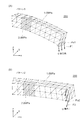
- FIG. 12 is a diagram for explaining the observation conditions used in the second embodiment.
- two sets of external force F and action point Pa are prepared.
- FIG. 12A shows a first set (pattern 1) of the external force F1 and the action point Pa1
- FIG. 12B shows a second set (pattern 2) of the external force F2 and the action point Pa2.
- the mesh model 200 shown in FIG. 12 represents the cubic block which has the elastic modulus E harder than the periphery by shading similarly to the case of FIG.
- the first external force F1 is applied downward ( ⁇ z-axis direction) with the three apexes at the lower right end of the mesh model 200 as the action points Pa1.
- the second set (pattern 2) shown in FIG. 12B, three apexes located on the left side of the right end of the mesh model 200 toward the end face are set to the left side ( ⁇ y axis direction) with the action point Pa2.
- transformation at the time of applying the 2nd external force F2 is represented.
- the action point Pa may be one and the action direction of the external force F may be plural. There may be two acting directions of the external force F.
- the information processing apparatus 10 obtains the observation displacement amount u o for each pattern, and thereafter, the difference between the observation displacement amount u o and the estimated displacement amount u o ′ for each pattern.
- the magnitude f1 of the external force F1 and the magnitude f2 of the external force F2 that minimize (u o ⁇ u o ′) and the distribution of the elastic modulus E over the entire mesh model 200 are obtained as optimal solutions.
- the optimization unit 115 obtains an unknown parameter that satisfies the following equation (Equation 9) as an optimal solution.
- U 0 is a matrix in which u 1o and u 2o are arranged in the column direction
- F is a matrix in which f 1 and f 2 are arranged in the column direction.
- the two-dimensional norm in the expression on the third row is a matrix norm, such as a Frobenius norm.
- FIG. 13 is a diagram illustrating experimental results when the pattern used for estimating the distribution of the elastic modulus E is one set (Embodiment 1) and when the pattern is two sets (Embodiment 2).
- the vertical axis in FIG. 13 is a mean square error (Root Mean Square Error: RMSE) between the true elastic modulus E and the estimated elastic modulus E ′, and the horizontal axis is the ratio of the number of observable vertices (see FIG. 9). is there.
- RMSE Root Mean Square Error
- the number of sets defined by the work point Pa and the magnitude f of the external force F is “2”, but the number of sets may be three or more.
- the estimation accuracy can be increased as the number of sets increases.
- the elastography method which is an example of a non-invasive method for evaluating a distortion image generated on an evaluation object (for example, an organ) by applying vibration such as ultrasonic waves
- an external force F applied to the evaluation object is timed. Changes. That is, in the elastography method, there are a plurality of sets defined by the action point Pa and the magnitude f of the external force F. Therefore, the present embodiment is compatible with the elastography method and can be estimated with high accuracy.
- the optimization unit 115 obtains an unknown parameter that satisfies the following equation (Equation 10) as an optimal solution.
- the second term of Equation 10 is a sparse term.
- E 0 is a reference value of the elastic modulus applied to most vertices.
- the sparse term is an expression for obtaining a one-dimensional norm L 1 for the difference (that is, ⁇ E) between the elasticity value E estimated for each vertex and the reference value.
- the coefficient ⁇ is set to 0.1.
- the sparse term has a small norm when the distribution of the estimated elastic modulus E distribution is high. Therefore, the distribution of the elastic modulus E having a large norm of the sparse term becomes low in evaluation.
- the value of the coefficient ⁇ is an example.
- FIG. 14 shows the case where the pattern used for estimating the distribution of the elastic modulus E is one set (Embodiment 1), the case where there are two patterns (Embodiment 2), and the case where there are two patterns (Embodiment). It is a figure which shows the experimental result when the sparsity of the change of the elasticity modulus E is added in the case of 2) (Embodiment 3).
- the vertical axis in FIG. 14 is the mean square error (Root Mean Square Error: RMSE) between the true elastic modulus E and the estimated elastic modulus E ′, and the horizontal axis is the ratio of the number of observable vertices (see FIG. 9). is there.
- RMSE Root Mean Square Error
- the sparsity of the change in the elastic modulus E when the sparsity of the change in the elastic modulus E is combined with the second embodiment, the first embodiment (when the number of sets is “1”) and the second embodiment It can be seen that the estimation accuracy can be improved for any of the cases of 2 (when the number of sets is “2”). In particular, when the sparsity of change in the elastic modulus E is combined with the second embodiment, high estimation accuracy can be obtained even when the ratio of the number of observable vertices is low.
- FIG. 15 is a diagram for explaining the relationship between the ratio of the number of observed vertices and the observation accuracy in the case of the present embodiment.
- the vertical axis in FIG. 15 is the elastic modulus, and the horizontal axis is the block number.
- FIG. 15 shows the case where the estimated number of blocks N is 40.
- the change in the true elastic modulus E is represented by a rectangular pulse, and the estimated change in the elastic modulus E is represented by a broken line.
- FIG. 15A when the number of observed vertices is 49% of the whole, the two waveforms are approximately the same.
- FIG. 15B when the number of observed vertices is 66% of the whole, The overlap between the two waveforms is even higher.
- the information processing system 100 can be used for a medical support system that supports diagnosis and surgery by a doctor, and can also be used for industrial fields other than the medical field, for observation and analysis purposes, and for production or manufacturing purposes.
- the information processing system 100 when used as a medical support system, as described above, since the visual field is limited, even if the whole image of the organ cannot be observed at once, the change in the organ that has occurred in the observable part Using the information (observation displacement u o ), the distribution of the elastic modulus E specific to the organ of the patient who is the subject can be estimated with high accuracy.
- the imaging camera 20 is an imaging unit that can capture the elastic body 1 that is an estimation target of the elastic modulus E as a moving image. May be. In this case, it may acquire the observation displacement u o described above with reference to the still image captured from a moving image captured.
- the shooting direction is not limited to one, and there may be a plurality of shooting directions. Also can increase the amount of information of the observation displacement u o by using an image obtained by photographing the deformation by external force F from a plurality of directions, thereby improving the estimation accuracy.
- Embodiment 1 the case where the estimated block number N is given as a fixed value has been described. However, the spatial resolution of the estimation result is gradually increased while the estimated block number N is increased.
- a technique may be adopted. That is, the estimation process for the distribution of the elastic modulus E may be divided into a plurality of steps. For example, in the first estimation step, the estimation process is executed for the case where the estimated number of blocks N is 10, the estimation result is obtained in a short time, and the estimation result is displayed on the display device 40. In the next estimation step, the estimation is performed. The number of blocks N may be increased to a predetermined value (for example, 20), and execution of the estimation process and update of the display of the estimation result may be repeated. According to such a method, the user can acquire an approximate image of the distribution of the elastic modulus E at an early stage and acquire it with higher spatial resolution as time passes.
- a predetermined value for example, 20
Landscapes
- Health & Medical Sciences (AREA)
- Life Sciences & Earth Sciences (AREA)
- Engineering & Computer Science (AREA)
- Medical Informatics (AREA)
- Public Health (AREA)
- General Health & Medical Sciences (AREA)
- Biomedical Technology (AREA)
- Pathology (AREA)
- Surgery (AREA)
- Physics & Mathematics (AREA)
- Animal Behavior & Ethology (AREA)
- Molecular Biology (AREA)
- Heart & Thoracic Surgery (AREA)
- Biophysics (AREA)
- Veterinary Medicine (AREA)
- Nuclear Medicine, Radiotherapy & Molecular Imaging (AREA)
- Radiology & Medical Imaging (AREA)
- Epidemiology (AREA)
- Primary Health Care (AREA)
- Oral & Maxillofacial Surgery (AREA)
- Dentistry (AREA)
- Physiology (AREA)
- Computer Vision & Pattern Recognition (AREA)
- Databases & Information Systems (AREA)
- Data Mining & Analysis (AREA)
- Bioinformatics & Cheminformatics (AREA)
- Chemical & Material Sciences (AREA)
- Medicinal Chemistry (AREA)
- Optics & Photonics (AREA)
- General Physics & Mathematics (AREA)
- Theoretical Computer Science (AREA)
- Ultra Sonic Daignosis Equipment (AREA)
- Magnetic Resonance Imaging Apparatus (AREA)
- Image Analysis (AREA)
Abstract
情報処理装置は、弾性体の一部分を撮像した画像から取得した観察変位量と弾性体の三次元モデルについて算出される推定変位量のうち観察領域に対応する領域部分の推定変位量との差分を最小化する最適解として、既知の作用点に作用する外力の大きさと当該三次元モデルにおける弾性率の分布とを求める演算部を有する。
Description
本発明は、情報処理装置、情報処理方法及びプログラムに関する。
癌病変に対する触診にみられるように、生体組織の硬さに関する情報は、医師が診断を下す上で有用である。近年では、臓器などの生体組織の弾性情報を定量的かつ客観的に評価し、その分布を画像表示するエラストグラフィ技術が実用化されている。エラストグラフィ技術には、例えば核磁気共鳴弾性計測法(Magnetic Resonance Elastography: MRE)や超音波エラストグラフィがある。
MREは、磁気共鳴画像(Magnetic Resonanse Imaging: MRI)を用いる弾性率測定法であり、計測対象を外部から振動させた状態で撮影し、対象物体内を伝播する振動波を画像化する手法である。超音波エラストグラフィは、計測対象に外圧を加えたときに生じる組織のひずみ分布を利用する方法や対象組織内にせん断波を生じさせ、その伝播速度を利用する方法に代表される手法である。
O. Goksel, H. Eskandari, and S. E. Salcudean, "Mesh adaptation for improving elasticity reconstruction using the FEM inverse problem,"IEEE Trans. Med. Imaging、 vol. 32、no. 2, pp. 408-418, 2013.p21-23
ところで、エラストグラフィ技術により弾性情報を取得できる領域範囲は、波が伝播する局所領域(対象組織の表面部分)や圧力を加えた領域の近傍範囲に限られる。
そこで、本発明は、局所的な変位情報から弾性体全体における弾性率の分布を推測する手法の提供を目的とする。
請求項1に記載の発明は、弾性体の一部分を撮像した画像から取得した観察変位量と当該弾性体の三次元モデルについて算出される推定変位量のうち観察領域に対応する領域部分の推定変位量との差分を最小化する最適解として、既知の作用点に作用する外力の大きさと当該三次元モデルにおける弾性率の分布とを求める演算部を有する情報処理装置である。
請求項2に記載の発明は、前記演算部は、次式に基づいて、前記外力の大きさと、前記弾性率の分布を求めることを特徴とする請求項1に記載の情報処理装置である。
 ここで、E*は、評価関数J(E,f)を最小にするEとfの集合であり、Eは、弾性率であり、E0は、弾性率の基準値であり、fは、外力の大きさであり、u0は、観察変位量であり、L0(E)は、弾性率Eで表現される全体剛性マトリクスKの逆行列成分のうち観察できる部分であり、L0(E)fは、推定変位量であり、λは、係数であり、|| ||1は、1次元のノルムであり、|| ||2は、2次元のノルムである。
請求項3に記載の発明は、弾性体の一部分を撮像した画像から観測変位量を取得する取得部と、前記弾性体に作用する外力の作用点を受け付ける受付部と、前記弾性体の三次元モデルにおける弾性率の分布と、前記外力の大きさとを変数として、当該三次元モデルの推定変位量を推定する推定部と、前記観測変位量と当該観測変位量に対応する前記推定変位量との差分を最小化する最適解として、前記外力の大きさと前記三次元モデルにおける前記弾性率の分布を求める最適化部とを有する情報処理装置である。
請求項4に記載の発明は、前記最適化部は、次式に基づいて、前記外力の大きさと、前記弾性率の分布を求めることを特徴とする請求項3に記載の情報処理装置である。
 ここで、E*は、評価関数J(E,f)を最小にするEとfの集合であり、Eは、弾性率であり、E0は、弾性率の基準値であり、fは、外力の大きさであり、u0は、観察変位量であり、L0(E)は、弾性率Eで表現される全体剛性マトリクスKの逆行列成分のうち観察できる部分であり、L0(E)fは、推定変位量であり、λは、係数であり、|| ||1は、1次元のノルムであり、|| ||2は、2次元のノルムである。
請求項5に記載の発明は、最適解として求められた前記弾性率の分布に基づいて前記三次元モデルを表現する表現部を更に有することを特徴とする請求項1又は3に記載の情報処理装置である。
請求項6に記載の発明は、前記画像は、単一の撮像カメラによって撮像された静止画像であることを特徴とする請求項1又は3に記載の情報処理装置である。
請求項7に記載の発明は、前記最適解は、前記弾性率の分布の初期値に対する変化量の絶対値和と前記差分との総和を最小化する値として求められることを特徴とする請求項1又は3に記載の情報処理装置である。
請求項8に記載の発明は、前記作用点の情報が複数与えられる場合、前記最適解は、個々の当該作用点について計算される前記差分の総和を最小化する値として求めることを特徴とする請求項1又は3に記載の情報処理装置である。
請求項9に記載の発明は、前記作用点に対して複数の前記外力が与えられる場合、前記最適解は、個々の当該外力について計算される前記差分の総和を最小化する値として求めることを特徴とする請求項1又は3に記載の情報処理装置である。
請求項10に記載の発明は、前記作用点は複数であり、当該作用点にはそれぞれ異なる前記外力が作用されることを特徴とする請求項1又は3に記載の情報処理装置である。
請求項11に記載の発明は、前記最適解を求める空間分解能を低い状態から徐々に高めることを特徴とする請求項1又は3に記載の情報処理装置である。
請求項12に記載の発明は、前記作用点に作用する前記外力の大きさが与えられる場合、前記最適解は、前記差分を最小化する前記弾性率の分布として求められることを特徴とする請求項1又は3に記載の情報処理装置である。
請求項13に記載の発明は、弾性体の一部分を撮像した画像から観察変位量を取得する処理と、前記弾性体に作用する外力の作用点を受け付ける処理と、前記弾性体の三次元モデルにおける弾性率の分布と、前記外力の大きさとを変数として、当該三次元モデルの推定変位量を推定する処理と、前記観測変位量と当該観測変位量に対応する前記推定変位量との差分を最小化する最適解として、前記外力の大きさと前記三次元モデルにおける前記弾性率の分布を求める処理とを有する情報処理方法である。
請求項14に記載の発明は、コンピュータに、弾性体の一部分を撮像した画像から観察変位量を取得する処理と、前記弾性体に作用する外力の作用点を受け付ける処理と、前記弾性体の三次元モデルにおける弾性率の分布と、前記外力の大きさとを変数として、当該三次元モデルの推定変位量を推定する処理と、前記観測変位量と当該観測変位量に対応する前記推定変位量との差分を最小化する最適解として、前記外力の大きさと前記三次元モデルにおける前記弾性率の分布を求める処理とを実行させるプログラムである。
請求項2に記載の発明は、前記演算部は、次式に基づいて、前記外力の大きさと、前記弾性率の分布を求めることを特徴とする請求項1に記載の情報処理装置である。
請求項3に記載の発明は、弾性体の一部分を撮像した画像から観測変位量を取得する取得部と、前記弾性体に作用する外力の作用点を受け付ける受付部と、前記弾性体の三次元モデルにおける弾性率の分布と、前記外力の大きさとを変数として、当該三次元モデルの推定変位量を推定する推定部と、前記観測変位量と当該観測変位量に対応する前記推定変位量との差分を最小化する最適解として、前記外力の大きさと前記三次元モデルにおける前記弾性率の分布を求める最適化部とを有する情報処理装置である。
請求項4に記載の発明は、前記最適化部は、次式に基づいて、前記外力の大きさと、前記弾性率の分布を求めることを特徴とする請求項3に記載の情報処理装置である。
請求項5に記載の発明は、最適解として求められた前記弾性率の分布に基づいて前記三次元モデルを表現する表現部を更に有することを特徴とする請求項1又は3に記載の情報処理装置である。
請求項6に記載の発明は、前記画像は、単一の撮像カメラによって撮像された静止画像であることを特徴とする請求項1又は3に記載の情報処理装置である。
請求項7に記載の発明は、前記最適解は、前記弾性率の分布の初期値に対する変化量の絶対値和と前記差分との総和を最小化する値として求められることを特徴とする請求項1又は3に記載の情報処理装置である。
請求項8に記載の発明は、前記作用点の情報が複数与えられる場合、前記最適解は、個々の当該作用点について計算される前記差分の総和を最小化する値として求めることを特徴とする請求項1又は3に記載の情報処理装置である。
請求項9に記載の発明は、前記作用点に対して複数の前記外力が与えられる場合、前記最適解は、個々の当該外力について計算される前記差分の総和を最小化する値として求めることを特徴とする請求項1又は3に記載の情報処理装置である。
請求項10に記載の発明は、前記作用点は複数であり、当該作用点にはそれぞれ異なる前記外力が作用されることを特徴とする請求項1又は3に記載の情報処理装置である。
請求項11に記載の発明は、前記最適解を求める空間分解能を低い状態から徐々に高めることを特徴とする請求項1又は3に記載の情報処理装置である。
請求項12に記載の発明は、前記作用点に作用する前記外力の大きさが与えられる場合、前記最適解は、前記差分を最小化する前記弾性率の分布として求められることを特徴とする請求項1又は3に記載の情報処理装置である。
請求項13に記載の発明は、弾性体の一部分を撮像した画像から観察変位量を取得する処理と、前記弾性体に作用する外力の作用点を受け付ける処理と、前記弾性体の三次元モデルにおける弾性率の分布と、前記外力の大きさとを変数として、当該三次元モデルの推定変位量を推定する処理と、前記観測変位量と当該観測変位量に対応する前記推定変位量との差分を最小化する最適解として、前記外力の大きさと前記三次元モデルにおける前記弾性率の分布を求める処理とを有する情報処理方法である。
請求項14に記載の発明は、コンピュータに、弾性体の一部分を撮像した画像から観察変位量を取得する処理と、前記弾性体に作用する外力の作用点を受け付ける処理と、前記弾性体の三次元モデルにおける弾性率の分布と、前記外力の大きさとを変数として、当該三次元モデルの推定変位量を推定する処理と、前記観測変位量と当該観測変位量に対応する前記推定変位量との差分を最小化する最適解として、前記外力の大きさと前記三次元モデルにおける前記弾性率の分布を求める処理とを実行させるプログラムである。
請求項1記載の発明によれば、変位量を取得できる領域が弾性体の一部分に限られる場合でも弾性体全域における弾性率の分布を求めることができる。
請求項2記載の発明によれば、変位量を取得できる領域が弾性体の一部分に限られる場合でも弾性体全域における弾性率の分布を求めることができる。
請求項3記載の発明によれば、変位量を取得できる領域が弾性体の一部分に限られる場合でも弾性体全域における弾性率の分布を求めることができる。
請求項4記載の発明によれば、変位量を取得できる領域が弾性体の一部分に限られる場合でも弾性体全域における弾性率の分布を求めることができる。
請求項5記載の発明によれば、弾性率の分布を三次元モデル上で視覚的に確認できる。
請求項6記載の発明によれば、弾性体の観察に使用する装置構成を簡素化できる。
請求項7記載の発明によれば、局在性が高い弾性率の分布を求めることができる。
請求項8記載の発明によれば、変位量の取得に用いた外力の作用点が1つだけの場合に比して推定精度を高めることができる。
請求項9記載の発明によれば、変位量の取得に用いた外力が1つだけの場合に比して推定精度を高めることができる。
請求項10記載の発明によれば、変位量の取得に用いた作用点と外力がそれぞれ1つだけの場合に比して推定精度を高めることができる。
請求項11記載の発明によれば、時間の経過とともに精度の高い推定結果を得ることができる。
請求項12記載の発明によれば、外力の大きさが与えられない場合と比して推定精度を高めることができる。
請求項13記載の発明によれば、変位量を取得できる領域が弾性体の一部分に限られる場合でも弾性体全域における弾性率の分布を求めることができる。
請求項14記載の発明によれば、変位量を取得できる領域が弾性体の一部分に限られる場合でも弾性体全域における弾性率の分布を求めることができる。
請求項2記載の発明によれば、変位量を取得できる領域が弾性体の一部分に限られる場合でも弾性体全域における弾性率の分布を求めることができる。
請求項3記載の発明によれば、変位量を取得できる領域が弾性体の一部分に限られる場合でも弾性体全域における弾性率の分布を求めることができる。
請求項4記載の発明によれば、変位量を取得できる領域が弾性体の一部分に限られる場合でも弾性体全域における弾性率の分布を求めることができる。
請求項5記載の発明によれば、弾性率の分布を三次元モデル上で視覚的に確認できる。
請求項6記載の発明によれば、弾性体の観察に使用する装置構成を簡素化できる。
請求項7記載の発明によれば、局在性が高い弾性率の分布を求めることができる。
請求項8記載の発明によれば、変位量の取得に用いた外力の作用点が1つだけの場合に比して推定精度を高めることができる。
請求項9記載の発明によれば、変位量の取得に用いた外力が1つだけの場合に比して推定精度を高めることができる。
請求項10記載の発明によれば、変位量の取得に用いた作用点と外力がそれぞれ1つだけの場合に比して推定精度を高めることができる。
請求項11記載の発明によれば、時間の経過とともに精度の高い推定結果を得ることができる。
請求項12記載の発明によれば、外力の大きさが与えられない場合と比して推定精度を高めることができる。
請求項13記載の発明によれば、変位量を取得できる領域が弾性体の一部分に限られる場合でも弾性体全域における弾性率の分布を求めることができる。
請求項14記載の発明によれば、変位量を取得できる領域が弾性体の一部分に限られる場合でも弾性体全域における弾性率の分布を求めることができる。
以下、添付図面を参照して、本発明の実施の形態について詳細に説明する。
<概念イメージ>
図1は、後述する実施の形態で採用する推定手法の概念イメージを説明する図である。図1に示すように、各実施の形態は、弾性体1の全体を観察できない場合(すなわち、観察できる部分と観察できない部分がある場合)を前提条件とし、各実施の形態では、観察できる部分における局所的な変位情報を用いて弾性体全体における弾性率の分布を推定する手法について記述する。
図1は、後述する実施の形態で採用する推定手法の概念イメージを説明する図である。図1に示すように、各実施の形態は、弾性体1の全体を観察できない場合(すなわち、観察できる部分と観察できない部分がある場合)を前提条件とし、各実施の形態では、観察できる部分における局所的な変位情報を用いて弾性体全体における弾性率の分布を推定する手法について記述する。
各実施の形態では、弾性体1を変形させる外力Fの作用点Paの位置情報が既知であることを利用して推定処理を実行する。
作用点Paの位置情報は、推定処理が始まる前に処理システムに与えられればよく、作用点Paの位置は任意である。従って、図1に示すように、作用点Paの位置が観察できる部分に存在する必要はない。
作用点Paの個数についての制限もなく、必ずしも1つである必要はない。従って、作用点Paの個数は、1個でも、複数個でも、弾性体1の表面全体でも良い。
作用点Paの位置情報は、推定処理が始まる前に処理システムに与えられればよく、作用点Paの位置は任意である。従って、図1に示すように、作用点Paの位置が観察できる部分に存在する必要はない。
作用点Paの個数についての制限もなく、必ずしも1つである必要はない。従って、作用点Paの個数は、1個でも、複数個でも、弾性体1の表面全体でも良い。
一方で、作用点Paに作用する外力Fの大きさfを与える情報や弾性体1が周囲に固定されている部位(固定点)Pfの位置情報は、既知であっても未知であっても良い。一般には、既知である情報が増えるほど、推定精度が高くなり、推定に要する計算時間も少なく済む。
図1では、観察できる部分と観察できない部分の説明のため、弾性体1の一部分が遮蔽物2によって覆われている様子を表しているが、弾性体1の一部分が遮蔽物2で覆われていることを必須とするものではない。例えば弾性体1を一方向のみから観察する場合、観察視野に含まれる部分が観察できる部分であり、観察視野に含まれない部分が観察できない部分となる。従って、観察方向から見て弾性体1の陰になる部分(例えば裏側や背面側)は、観察できない部分の一例である。
また、後述する実施の形態では、弾性体1のうち観察できる部分の変位量は、部位毎に特定できるものとする。すなわち、外力Fの作用による弾性体1の変位量は既知の情報として処理システムに与えられるものとする。
変位量は、観察手段の違いにより、弾性体1の表面領域についてのみ与えられる場合と弾性体1の内部領域も含めて与えられる場合がある。一般には、変位量が特定された領域が多いほど(観察できる部分の割合が増えるほど)、弾性率の推定精度が高くなる。
変位量は、観察手段の違いにより、弾性体1の表面領域についてのみ与えられる場合と弾性体1の内部領域も含めて与えられる場合がある。一般には、変位量が特定された領域が多いほど(観察できる部分の割合が増えるほど)、弾性率の推定精度が高くなる。
<用語>
各実施の形態における弾性率には、押込・引張方向についての硬さを表すヤング率E、せん断方向についての硬さを表す剛性率G、ポアソン比ν、体積弾性率Kなどが含まれ、後述する実施の形態では、弾性率がヤング率であるものとして使用する。
各実施の形態において、弾性体1とは、外力Fの作用により歪が生じる(変形する)一方、外力Fの作用が停止されると元の寸法に戻る性質を有する物質をいうものとする。本実施の形態では、例えば生体組織における各種の臓器などの近似的にフックの法則を用いて表現される弾性体を想定する。
もっとも、各実施の形態では、弾性体1における弾性率の分布が一様でない場合を想定する。ここで、弾性率の分布が一様でない場合とは、例えば弾性体1の少なくとも一部の弾性率が周囲の弾性率と異なることをいう。
各実施の形態における弾性率には、押込・引張方向についての硬さを表すヤング率E、せん断方向についての硬さを表す剛性率G、ポアソン比ν、体積弾性率Kなどが含まれ、後述する実施の形態では、弾性率がヤング率であるものとして使用する。
各実施の形態において、弾性体1とは、外力Fの作用により歪が生じる(変形する)一方、外力Fの作用が停止されると元の寸法に戻る性質を有する物質をいうものとする。本実施の形態では、例えば生体組織における各種の臓器などの近似的にフックの法則を用いて表現される弾性体を想定する。
もっとも、各実施の形態では、弾性体1における弾性率の分布が一様でない場合を想定する。ここで、弾性率の分布が一様でない場合とは、例えば弾性体1の少なくとも一部の弾性率が周囲の弾性率と異なることをいう。
<実施の形態1>
<システム構成>
図2は、情報処理システム100のハードウェア構成例を示す図である。
情報処理システム100は、弾性体1(図1参照)の弾性率の分布を推定する演算処理を実行する情報処理装置10と、弾性体1の撮像に用いる少なくとも1つの撮像カメラ20と、弾性体1のメッシュモデルの作成に使用する三次元画像データ(ボリュームデータ)を記憶する三次元画像データ記憶装置30と、推定された弾性率の分布の表示等に用いる表示装置40と、ユーザが操作するマウスやポインティングデバイス等で構成される入力装置50とを有している。
<システム構成>
図2は、情報処理システム100のハードウェア構成例を示す図である。
情報処理システム100は、弾性体1(図1参照)の弾性率の分布を推定する演算処理を実行する情報処理装置10と、弾性体1の撮像に用いる少なくとも1つの撮像カメラ20と、弾性体1のメッシュモデルの作成に使用する三次元画像データ(ボリュームデータ)を記憶する三次元画像データ記憶装置30と、推定された弾性率の分布の表示等に用いる表示装置40と、ユーザが操作するマウスやポインティングデバイス等で構成される入力装置50とを有している。
情報処理装置10は、いわゆるコンピュータであり、プログラムを実行するCPU(Central Processing Unit)11と、BIOS(Basic Input / Output System)やファームウェアなどのプログラムやデータを記憶するROM(Read Only Memory)12と、プログラムに作業エリアを与えるRAM(Random Access Memory)13と、処理対象とする画像データを記憶する記憶部14とにより構成される。記憶部14は、ハードディスク装置や半導体メモリなどの記憶装置である。CPU11によるプログラムの実行を通じて実現される機能については後述する。
撮像カメラ20は、弾性体1の観察に使用される撮像装置である。撮像カメラ20は、弾性体1の観察に適した撮像装置であればよい。例えば撮像カメラ20には、赤外線カメラ、内視鏡カメラ、超音波イメージング装置、光超音波イメージング装置などを使用する。
赤外線カメラや内視鏡カメラを用いる場合、情報処理装置10は、弾性体1の表面に存在する特徴点や赤外線マーカーの移動を通じて各部位の変位量を特定することができる。超音波イメージング装置を用いる場合、情報処理装置10は、弾性体1の内部も含めて各部位の変位量を特定することができる。なお、内視鏡カメラの撮像素子は、CCD(Charge Coupled Device)でもCMOS(Complementary MOS)でもよい。
本実施の形態では、単一の撮像カメラ20を使用し、弾性体1を一方向から撮影した静止画像を出力する。
赤外線カメラや内視鏡カメラを用いる場合、情報処理装置10は、弾性体1の表面に存在する特徴点や赤外線マーカーの移動を通じて各部位の変位量を特定することができる。超音波イメージング装置を用いる場合、情報処理装置10は、弾性体1の内部も含めて各部位の変位量を特定することができる。なお、内視鏡カメラの撮像素子は、CCD(Charge Coupled Device)でもCMOS(Complementary MOS)でもよい。
本実施の形態では、単一の撮像カメラ20を使用し、弾性体1を一方向から撮影した静止画像を出力する。
三次元画像データ記憶装置30は、弾性体1を断層撮影することにより取得した断層画像データを積み重ねるように再構成した画像(再構成画像)を三次元画像データとして記憶する大容量のハードディスク装置等で構成される。
三次元画像データ記憶装置30は、情報処理装置10に対して直接接続される場合だけでなく、ネットワーク上にサーバやネットワークストレージとして存在してもよい。ここで、断層画像データの取得には、例えばCT(Computed Tomography)、PET(Positron Emission Tomography)、MRI等を使用する。
三次元画像データ記憶装置30は、情報処理装置10に対して直接接続される場合だけでなく、ネットワーク上にサーバやネットワークストレージとして存在してもよい。ここで、断層画像データの取得には、例えばCT(Computed Tomography)、PET(Positron Emission Tomography)、MRI等を使用する。
表示装置40は、例えば液晶ディスプレイで構成される。液晶ディスプレイは、液晶パネル、バックライトなどで構成される。なお、表示装置40は、有機EL(ElectroLuminescence)ディスプレイ等でもよい
図3は、CPU11によるコンピュータプログラムの実行を通じて実現される機能構成例を説明する図である。
処理機能の観点から見た情報処理装置10は、三次元のメッシュモデルを生成するメッシュモデル生成部111と、撮像カメラ20から出力されるカメラ画像から観察部位についての変位量(観察変位量uo)を取得する観察変位量取得部112と、作用点Paの位置情報を受け付ける作用点受付部113と、作用点情報をメッシュモデルに適用してメッシュモデルの各部位における変位量(推定変位量uo’)を計算する変位量推定部114と、推定変位量uo’と観察変位量uoとの差分を最小化する弾性率E(結果として弾性率Eの関数である要素剛性マトリクスK)と外力Fの大きさfを最適解として求める最適化部115と、最適解とする要素剛性マトリクスKから特定される弾性率の分布をメッシュモデルに重ねて表現した画像を生成して表示装置40に出力する表現部116とを有している。これらの機能部は、請求の範囲における「演算部」の一例である。
処理機能の観点から見た情報処理装置10は、三次元のメッシュモデルを生成するメッシュモデル生成部111と、撮像カメラ20から出力されるカメラ画像から観察部位についての変位量(観察変位量uo)を取得する観察変位量取得部112と、作用点Paの位置情報を受け付ける作用点受付部113と、作用点情報をメッシュモデルに適用してメッシュモデルの各部位における変位量(推定変位量uo’)を計算する変位量推定部114と、推定変位量uo’と観察変位量uoとの差分を最小化する弾性率E(結果として弾性率Eの関数である要素剛性マトリクスK)と外力Fの大きさfを最適解として求める最適化部115と、最適解とする要素剛性マトリクスKから特定される弾性率の分布をメッシュモデルに重ねて表現した画像を生成して表示装置40に出力する表現部116とを有している。これらの機能部は、請求の範囲における「演算部」の一例である。
メッシュモデル生成部111は、三次元画像データ記憶装置30から観察対象とする弾性体1の三次元画像データを取り込むと、連続体として与えられた三次元画像データから単純な形状要素の集合体であるメッシュモデルを生成する機能部である。ここでのメッシュモデルは三次元モデルの一例であり、最小要素は立方体や四面体(三角錐)で表現される。
図4は、弾性体1をメッシュ構造で表現したメッシュモデル200の例を示す図である。図4は、外力F(図5参照)が作用点Pa(図5参照)に加えられる前のメッシュモデル200を表している。図中の丸印は最小要素のノードを示す。なお、図5は、メッシュモデル200の右端下部を作用点Paとして外力Fを加えて弾性変形させた後のメッシュモデル200を表している。
観察変位量取得部112は、外力Fが作用点Paに加えられる前のカメラ画像と外力Fが作用点Paに加えられた後のカメラ画像とを比較して画像内に現れる各部位の観察変位量uoを取得する機能部である。
なお、観察変位量取得部112で取得される観察変位量uoは、カメラ画像上で特定される各位置についての変位量であり、メッシュモデル200を構成するボクセルとの位置関係は不明である。
なお、観察変位量取得部112で取得される観察変位量uoは、カメラ画像上で特定される各位置についての変位量であり、メッシュモデル200を構成するボクセルとの位置関係は不明である。
そこで、観察変位量取得部112には、三次元画像データ又はメッシュモデル200(図4参照)とカメラ画像をマッチングし、観察変位量uoをメッシュモデル200の個々の頂点に対応付ける処理機能が用意されている。ここでの対応付けの際には、三次元画像データ又はメッシュモデル200の寸法とカメラ画像の寸法とを揃える処理も実行される。
一般には、三次元画像データ又はメッシュモデル200に含まれる画像情報が多いほどカメラ画像とのマッチング精度が高くなる。例えばメッシュモデル200をマッチングに使用する場合、メッシュモデル200の表面に三次元画像データの表面情報をレンダリングしたレンダリング画像をカメラ画像の輝度情報と比較すれば、メッシュモデル200の頂点に高いマッチング精度で観察変位量uoを対応付けることができる。
作用点受付部113は、作用点Paの位置情報を、入力装置50を通じて受け付ける機能部である。作用点受付部113は、例えばクリック操作が検出された際に、マウスカーソルが位置していたメッシュモデル200上の部位を外力Fの作用点Paとして受け付ける。
作用点受付部113は、受け付けた作用点Paの位置を、メッシュモデル200上の頂点の識別番号で特定し、変位量推定部114に出力する。
作用点受付部113は、受け付けた作用点Paの位置を、メッシュモデル200上の頂点の識別番号で特定し、変位量推定部114に出力する。
変位量推定部114は、線形有限要素法で使用する力の釣り合い式(すなわち、フックの法則を表現する式)を用いて、メッシュモデル200を構成する全ての頂点について推定変位量uo’を計算する機能部である。
具体的には、変位量推定部114は、メッシュモデル200の各頂点に加わる外力Fの大きさをf、各頂点における推定変位量をuo’、全体剛性マトリクスをKとする力の釣り合い式(f=K・uo’)を変形した式1に基づいて、推定変位量uo’を計算する。
 なお、添え字のoは、観測できる部分に位置する頂点を意味し、Lは、全体剛性マトリクスKの逆行列(K-1)を意味する。
具体的には、変位量推定部114は、メッシュモデル200の各頂点に加わる外力Fの大きさをf、各頂点における推定変位量をuo’、全体剛性マトリクスをKとする力の釣り合い式(f=K・uo’)を変形した式1に基づいて、推定変位量uo’を計算する。
本実施の形態の場合、弾性体1の弾性率Eの分布と弾性体1に加わる外力Fの大きさf(ベクトル)が最終的な推定対象となる。なお、弾性率Eは、全体剛性マトリクスKの内包パラメータであるので、全体剛性マトリクスKが特定されれば、弾性率Eも特定される。
以下では、説明を簡単にするために、全体剛性マトリクスKと弾性率Eの分布との関係を、図6を用いて説明する。図6は、二次元のメッシュモデルである。言うまでもなく、情報処理システム100で扱うのは、三次元のメッシュモデル200である。
図6に示すメッシュモデルの場合、三角形の要素Iは頂点番号1、2及び3で規定され、三角形の要素IIは頂点番号2、3及び4で規定される。このとき、頂点番号iに作用する力fi(i=1~4)と頂点番号iにおける変位量ui(i=1~4)は、全体剛性マトリクスKを用いた線形有限要素法での力の釣り合い式(式2)として与えられる。

ここで、個々の頂点番号i(i=1~4)に作用する外力Fの大きさfi(i=1~4)とその変位量ui(i=1~4)との関係付けに用いる要素剛性マトリクスKeは、以下の式3により導出される。
 ここで、Vは三角形の要素の体積である。
また、Bマトリクスは、要素の形状関数から求まるマトリクスであり、Dマトリクスは、弾性率Eとポアソン比νから求まるマトリクスである。
また、Bマトリクスは、要素の形状関数から求まるマトリクスであり、Dマトリクスは、弾性率Eとポアソン比νから求まるマトリクスである。
Dマトリクスは、次式(式4)により表すことができる。
 式4から分かるように、Dマトリクスは弾性率Eの関数である。従って、要素剛性マトリクスKeも弾性率Eの関数として表現される。
全体剛性マトリクスKは、三角形の要素Iの要素剛性マトリクスKeと、三角形の要素IIの要素剛性マトリクスKeとの和で与えられる。すなわち、全体剛性マトリクスKは、頂点番号1、2、3で構成される三角形の要素Iの要素剛性マトリクスKeと、頂点番号2、3、4で構成される三角形の要素IIの要素剛性マトリクスKeとの和で表される。
図6に示すように、三角形の要素Iと三角形の要素IIとでは、互いに重なり合う頂点が存在する。そこで、重なり合う各頂点に対して要素剛性マトリクスKeの重ね合わせを行う。
図7は、要素剛性マトリクスKeの重ね合わせ処理の概念を説明する図である。図7は、全体剛性マトリクスKが、要素Iの要素剛性マトリクスKeと要素IIの要素剛性マトリクスKeとの和で表されることを示している。前述したように、要素剛性マトリクスKeは弾性率Eの関数であったので、その和で表される全体剛性マトリクスKも弾性率Eの関数となる。
従って、本実施の形態におけるメッシュモデル200における全体剛性マトリクスKも弾性率Eの関数となる。
図7は、要素剛性マトリクスKeの重ね合わせ処理の概念を説明する図である。図7は、全体剛性マトリクスKが、要素Iの要素剛性マトリクスKeと要素IIの要素剛性マトリクスKeとの和で表されることを示している。前述したように、要素剛性マトリクスKeは弾性率Eの関数であったので、その和で表される全体剛性マトリクスKも弾性率Eの関数となる。
従って、本実施の形態におけるメッシュモデル200における全体剛性マトリクスKも弾性率Eの関数となる。
ところで、本実施の形態のカメラ画像は、前述したように、作用点Paは既知であるが大きさfが未知の外力Fによって弾性変形された弾性体1の一部分を撮像した画像である。
従って、式2のうち未知のパラメータは、弾性率Eの分布(全体剛性マトリクスK)と外力Fの大きさf(ベクトル)となる。
従って、式2のうち未知のパラメータは、弾性率Eの分布(全体剛性マトリクスK)と外力Fの大きさf(ベクトル)となる。
そこで、変位量推定部114では、これら未知のパラメータにそれぞれ任意の値を設定して推定変位量uo’を計算する。なお、推定変位量uo’の初回推定時には、変位量推定部114は、未知パラメータである弾性率Eの分布(全体剛性マトリクスK)と外力Fの大きさfのそれぞれに初期値を与えて推定変位量uo’を計算する。
式2をマトリクスで表現すると、次式(式5)となる。
 ここで、uo’は観察できる部分の推定変位量であり、ui’は観察できない部分の推定変位量である。また、Loは弾性率Eで表現される全体剛性マトリクスKの逆行列成分のうち観察できる部分であり、Liは弾性率Eで表現される全体剛性マトリクスKの逆行列成分のうち観察できない部分である。foは観察できる部分の頂点に作用する外力Fの大きさ、fiは観察できない部分の頂点に作用する外力Fの大きさである。
観察できる部分の推定変位量uo’に着目すると、式5は、次式(式6)として表現できる。
 ここで、作用点Paが既知であるので、外力Fの大きさfのうち作用点Pa以外の頂点に対応する外力Fの大きさを0(ゼロ)で表すことができる。
変位量推定部114は、この式6を用いて弾性率Eで表される成分Loと外力Fの大きさfにより推定変位量uo’(初期値を含む)を計算する。
変位量推定部114は、この式6を用いて弾性率Eで表される成分Loと外力Fの大きさfにより推定変位量uo’(初期値を含む)を計算する。
最適化部115は、メッシュモデル200の全ての頂点番号(観察できる部分だけでなく観察できない部分の頂点も含む)について推定された推定変位量uo’と、撮像カメラ20によって撮像された部分画像から特定された観察変位量uoとの差分を最小化する全体剛性マトリクスK(すなわち弾性率Eの分布)と外力fが得られるまで、未知パラメータの組み合わせを更新する。
具体的には、最適化部115は、推定変位量uo’と観察変位量uoとの差分を最小化する(すなわち、観察結果に最も近い変形を与える)未知パラメータを求める最適化問題を解く処理を実行する。当該処理を式で表すと次式(式7)となる。
 ここでのE*は、評価関数J(E,f)を最小にするEとfの集合を意味する。
本実施の形態の場合、評価関数J(E,f)は、推定変位量uo’と観察変位量uoの差分のL2ノルムで与えられる。
本実施の形態の場合、評価関数J(E,f)は、推定変位量uo’と観察変位量uoの差分のL2ノルムで与えられる。
最適化部115は、評価関数Jの最小値が求まるまで、未知パラメータEとfを更新し、更新された値を変位量推定部114にフィードバックする。すなわち、未知パラメータEとfの更新値を用いた変位量推定部114による推定変位量uo’の再計算と、最適化部115による推定変位量uo’の評価とが、評価関数Jの最小値が求まるまで繰り返し実行される。
本実施の形態では、最適化問題を解く手法として、共分散行列適応進化戦略(Covariance Matrix Adaptation Evolution Strategy:CMA-ES)を使用した。もっとも、最適化問題を解く手法には既知の他の手法を用いてもよい。例えば勾配法、モンテカルロ法、焼きなまし法などを用いてもよい。
なお、図3では、変位量推定部114と最適化部115を別の機能部として描画しているが、一つの機能部に含めてもよい。
なお、図3では、変位量推定部114と最適化部115を別の機能部として描画しているが、一つの機能部に含めてもよい。
表現部116(図3参照)は、最適解として特定された弾性率Eの分布と外力Fの大きさのうち弾性率Eの分布を、メッシュモデル200に重ねて表現した画像を表示装置40(図2参照)に表示する。弾性率Eの分布がメッシュモデル200と関連付けて表現されることにより、ユーザは、観察できない部分も含めた弾性体1の弾性率Eの分布を視覚的に理解できる。
なお、表現部116は、弾性率Eの違いを色や輝度の違いとして表現する。また、表現部116は、メッシュモデル200の各部に対応する弾性率Eの数値を表示してもよい。なお、表現部116は、必要に応じ、最適解として求まった外力Fの大きさfを出力する。
なお、表現部116は、弾性率Eの違いを色や輝度の違いとして表現する。また、表現部116は、メッシュモデル200の各部に対応する弾性率Eの数値を表示してもよい。なお、表現部116は、必要に応じ、最適解として求まった外力Fの大きさfを出力する。
<シミュレーション実験による検証>
以下では、弾性体1について作成したメッシュモデル200(すなわち、図4に示すメッシュモデル)と、弾性体1を局所的に観察して得られる観察変位量uoと、弾性体1に作用する外力Fの作用点Paの情報とを用いて推定した弾性率Eの分布の精度を検証した結果について説明する。
以下では、弾性体1について作成したメッシュモデル200(すなわち、図4に示すメッシュモデル)と、弾性体1を局所的に観察して得られる観察変位量uoと、弾性体1に作用する外力Fの作用点Paの情報とを用いて推定した弾性率Eの分布の精度を検証した結果について説明する。
以下では、シミュレーション実験では、弾性体1に対応するメッシュモデル200がN個の頂点を有するものとし、そのうちのM個(N>M)の頂点の観察変位量uoを用いて弾性体1全体の弾性率Eの分布を推定する場合に、観測できる頂点の数が推定精度に与える影響について説明する。
シミュレーション実験では、Visual C/C++を用いて、実施の形態に係る手法をプログラムとして記述し、作成されたプログラムを汎用計算機(OS:Windows 10 Pro、CPU:IntelCorei7-6700K、メモリ:16GB)で実行した。
なお、シミュレーションは、直方体形状のメッシュモデル200(図5参照)について実行した。このメッシュモデル200は、全体で99個の頂点を有し、最小要素を四面体とする。
なお、シミュレーションは、直方体形状のメッシュモデル200(図5参照)について実行した。このメッシュモデル200は、全体で99個の頂点を有し、最小要素を四面体とする。
また、図5に示すように、メッシュモデル200の左端に位置する9個の頂点を固定端Pfとし、それ以外の点を自由点とした。
さらに、図5に示すように、外力Fの作用点Paとして、メッシュモデル200の右端下部に位置する3個の頂点を指定した。これら3個の頂点には、同じ大きさfの外力Fがいずれも下向き(-z軸方向)に作用するものとした。
さらに、図5に示すように、外力Fの作用点Paとして、メッシュモデル200の右端下部に位置する3個の頂点を指定した。これら3個の頂点には、同じ大きさfの外力Fがいずれも下向き(-z軸方向)に作用するものとした。
メッシュモデル200の外力Fによる変形は、弾性体1の内部構造を与える弾性率Eの分布状態に依存する。ここでは、本実施の形態で提案する手法によって推定された弾性率Eの分布の推定精度を評価するために使用する真値としての内部構造について説明する。図8は、真値として使用する弾性率Eの分布をメッシュモデル200に重ねて表した図である。図8に示すメッシュモデル200は、一部分の弾性率Eだけが大きく(硬く)、他の部分の弾性率Eは同じ値を採る。図中、白丸のノードは観察できる部分に位置することを表し、黒丸のノードは観察できない部分に位置することを表している。
図8に示すメッシュモデル200は、40個の立方体ブロックのうち右端から左方向(-x方向)に7番目と8番目の左列に位置する4個の立方体ブロックの弾性率Eが2.0[MPa]と硬く、他の部分の弾性率Eが1.0[MPa]である場合を示している。
シミュレーション実験では、図8に示すメッシュモデル200に外力Fを作用させた場合に観測されたカメラ画像と作用点Paの位置に基づいて、メッシュモデル200の全ての頂点の弾性率Eの分布を推定した。
シミュレーション実験では、図8に示すメッシュモデル200に外力Fを作用させた場合に観測されたカメラ画像と作用点Paの位置に基づいて、メッシュモデル200の全ての頂点の弾性率Eの分布を推定した。
なお、図8に示すメッシュモデル200は、図5の説明と同じく、弾性体1のメッシュモデル200の右端下部にある3個の頂点に下方向(-z軸方向)へ10Nの外力Fを作用させて変形した状態を表している。勿論、情報処理装置10にとっては、外力Fの大きさfも未知パラメータである。
前述したように、シミュレーション実験の目的は、観測できる頂点の数が弾性率Eの推定精度に与える影響を評価することである。
そこで、シミュレーション実験では、観察できる頂点の数(観察変位量u0が与えられる頂点の数)が全体の10%の場合、20%の場合、…90%の場合について評価した。図9は、メッシュモデル200のうち観察できる頂点の数の割合を説明する図である。図9は、メッシュモデル200を横方向(x-z平面)から観察した図であり、x軸方向について10個の小区分に分割されている。このうち1つの小区分を観察する場合が全体の10%を観察する場合に相当し、2つの小区分を観察する場合が全体の20%を観察する場合に相当する。以下同様に、9つの小区分を観察する場合が全体の90%を観察する場合に相当する。
そこで、シミュレーション実験では、観察できる頂点の数(観察変位量u0が与えられる頂点の数)が全体の10%の場合、20%の場合、…90%の場合について評価した。図9は、メッシュモデル200のうち観察できる頂点の数の割合を説明する図である。図9は、メッシュモデル200を横方向(x-z平面)から観察した図であり、x軸方向について10個の小区分に分割されている。このうち1つの小区分を観察する場合が全体の10%を観察する場合に相当し、2つの小区分を観察する場合が全体の20%を観察する場合に相当する。以下同様に、9つの小区分を観察する場合が全体の90%を観察する場合に相当する。
ところで、弾性率Eの推定精度は、推定空間の次元数の影響を受けると予想される。ここで、推定空間の次元数とは、弾性率Eの推定解像度で表現される。例えば推定空間の次元数が低いことは低解像度で推定することを意味し、次元数が高いことは高解像度で推定することを意味する。換言すると、推定空間の次元数は、1つのメッシュモデル200を何個の単位区画(ブロック)に分割するかを表している。
以下のシミュレーション実験では弾性率Eの推定解像度を表す推定ブロック数Nを10個とする場合、N=20とする場合、N=40とする場合について検討した。
図10は、推定ブロック数Nと弾性率Eが推定される単位区画(ブロック)の大きさとの関係を説明する図である。
図10は、推定ブロック数Nと弾性率Eが推定される単位区画(ブロック)の大きさとの関係を説明する図である。
例えばN=10の場合は、メッシュモデル200(図9参照)を10個の単位区画(ブロック)で表現することを意味し、N=20の場合は、メッシュモデル200を20個の単位区画(ブロック)で表現することを意味し、N=40の場合は、メッシュモデル200を40個の単位区画(ブロック)で表現することを意味する。
つまり、N=40の場合の単位区画(ブロック)は、図8において説明した立方体ブロックと同じ形状になる。当然ながら推定ブロック数Nの値が大きいほど(推定される単位区画の大きさが小さいほど)空間分解能が高くなり、弾性率Eの分布を高精細に推定できる。
つまり、N=40の場合の単位区画(ブロック)は、図8において説明した立方体ブロックと同じ形状になる。当然ながら推定ブロック数Nの値が大きいほど(推定される単位区画の大きさが小さいほど)空間分解能が高くなり、弾性率Eの分布を高精細に推定できる。
続いて、推定ブロック数Nと高い推定精度を得るために必要とされる観察点数の割合との関係を説明する。後述するように、推定ブロック数Nが大きいほど(推定される単位区画の大きさが小さいほど)、高い推定精度を得るにはより多くの割合で弾性体1を観察することが必要になる。
図11は、推定ブロック数Nが10個の場合、20個の場合、40個の場合の実験結果を示す図である。図11の縦軸は真の弾性率Eと推定された弾性率E’との平均二乗誤差(Root Mean Square Error: RMSE)であり、横軸は観察できる頂点数の全体に占める割合(図9参照)である。
勿論、弾性率E’の推定に際しては、前述したように、メッシュモデル200の全ての頂点に同じ値の弾性率Eを与えた状態で最適解を求める推定処理が開始される。

図11は、推定ブロック数Nが10個の場合、20個の場合、40個の場合の実験結果を示す図である。図11の縦軸は真の弾性率Eと推定された弾性率E’との平均二乗誤差(Root Mean Square Error: RMSE)であり、横軸は観察できる頂点数の全体に占める割合(図9参照)である。
勿論、弾性率E’の推定に際しては、前述したように、メッシュモデル200の全ての頂点に同じ値の弾性率Eを与えた状態で最適解を求める推定処理が開始される。
図11によれば、メッシュモデル200を10個のブロックで表現する場合(低解像度で推定する場合)には、観測できる頂点の数がメッシュモデル200全体の15%程度でも高精度で弾性率Eを推定できることが分かる。また、この場合にはブロック数が少ないので、計算コストも低く済む。
また、メッシュモデル200を20個のブロックで表現する場合(中解像度で推定する場合)には、観測できる頂点の数がメッシュモデル200全体の50%程度になると高精度で弾性率Eを推定できることが分かる。
メッシュモデル200を40個のブロックで表現する場合(高解像度で推定する場合)には、観測できる頂点の数がメッシュモデル200全体の70%程度にならなければ最小二乗誤差が十分に小さくならないことが分かる。なお、ここでの低解像度、中解像度、高解像度は、単に3つの解像度間の相対的な関係を表したものにすぎない。
また、メッシュモデル200を20個のブロックで表現する場合(中解像度で推定する場合)には、観測できる頂点の数がメッシュモデル200全体の50%程度になると高精度で弾性率Eを推定できることが分かる。
メッシュモデル200を40個のブロックで表現する場合(高解像度で推定する場合)には、観測できる頂点の数がメッシュモデル200全体の70%程度にならなければ最小二乗誤差が十分に小さくならないことが分かる。なお、ここでの低解像度、中解像度、高解像度は、単に3つの解像度間の相対的な関係を表したものにすぎない。
<小括>
以上の通り、実施の形態1によれば、弾性体1の一部分(例えば全体の50%)を撮像した画像から取得した観察変位量uoと弾性体1のメッシュモデル200について算出される推定変位量uo’のうち観察領域に対応する領域部分の推定変位量との差分(uo-uo’)を最小化する最適解として、既知の作用点Paに作用する外力Fの大きさfとメッシュモデル200全域における弾性率Eの分布とを求めることにより、観察変位量uoを取得できる領域が弾性体1の一部分に限られる場合でも弾性体1全域における弾性率Eの分布を求めることができる。
以上の通り、実施の形態1によれば、弾性体1の一部分(例えば全体の50%)を撮像した画像から取得した観察変位量uoと弾性体1のメッシュモデル200について算出される推定変位量uo’のうち観察領域に対応する領域部分の推定変位量との差分(uo-uo’)を最小化する最適解として、既知の作用点Paに作用する外力Fの大きさfとメッシュモデル200全域における弾性率Eの分布とを求めることにより、観察変位量uoを取得できる領域が弾性体1の一部分に限られる場合でも弾性体1全域における弾性率Eの分布を求めることができる。
また、推定精度は、推定空間の解像度と観察できる頂点の割合に依存し、もし高解像度で弾性体1の弾性率Eを推定したい場合には、撮像カメラ20によって撮像される弾性体1の面積を広くする必要があり、低解像で弾性体1の弾性率Eを推定したい場合には、撮像カメラ20によって撮像される弾性体1の面積は狭くてもよい。
<実施の形態2>
本実施の形態では、前述した実施の形態1に比して、弾性率Eの分布の推定精度を高めるための手法について説明する。
図12は、実施の形態2で使用する観察条件を説明する図である。本実施の形態では、外力Fと作用点Paの組を2組用意する。図12(A)は、外力F1と作用点Pa1の第1の組(パターン1)を示し、図12(B)は、外力F2と作用点Pa2の第2の組(パターン2)を示す。
なお、図12に示すメッシュモデル200は、図8の場合と同じく、周囲より硬い弾性率Eを有する立方体ブロックを網掛けで表現している。
本実施の形態では、前述した実施の形態1に比して、弾性率Eの分布の推定精度を高めるための手法について説明する。
図12は、実施の形態2で使用する観察条件を説明する図である。本実施の形態では、外力Fと作用点Paの組を2組用意する。図12(A)は、外力F1と作用点Pa1の第1の組(パターン1)を示し、図12(B)は、外力F2と作用点Pa2の第2の組(パターン2)を示す。
なお、図12に示すメッシュモデル200は、図8の場合と同じく、周囲より硬い弾性率Eを有する立方体ブロックを網掛けで表現している。
図12(A)に示す第1の組(パターン1)は、メッシュモデル200の右端下部の3つの頂点を作用点Pa1として、下向き(-z軸方向)に第1の外力F1を作用させた場合の変形を表している。図12(B)に示す第2の組(パターン2)は、メッシュモデル200の右端のうち端面に向かって左辺に位置する3つの頂点を作用点Pa2として、左向きに(-y軸方向)に第2の外力F2を作用させた場合の変形を表している。
なお、図12においては、作用点Paだけでなく外力Fが作用する方向も異なる例を示しているが、作用点Paは1つで外力Fの作用方向が複数でもよいし、作用点Paは2つで外力Fの作用方向は1つでもよい。
この場合も、実施の形態1の場合と同様、情報処理装置10は、各パターンについての観察変位量uoを求め、その後、それぞれについて観察変位量uoと推定変位量uo’との差分(uo-uo’)を最小化する外力F1の大きさf1と外力F2の大きさf2と、メッシュモデル200全域における弾性率Eの分布を最適解として求める。
この場合も、実施の形態1の場合と同様、情報処理装置10は、各パターンについての観察変位量uoを求め、その後、それぞれについて観察変位量uoと推定変位量uo’との差分(uo-uo’)を最小化する外力F1の大きさf1と外力F2の大きさf2と、メッシュモデル200全域における弾性率Eの分布を最適解として求める。
すなわち、最適化部115は、次式(式9)を満たす未知パラメータを最適解として求める。
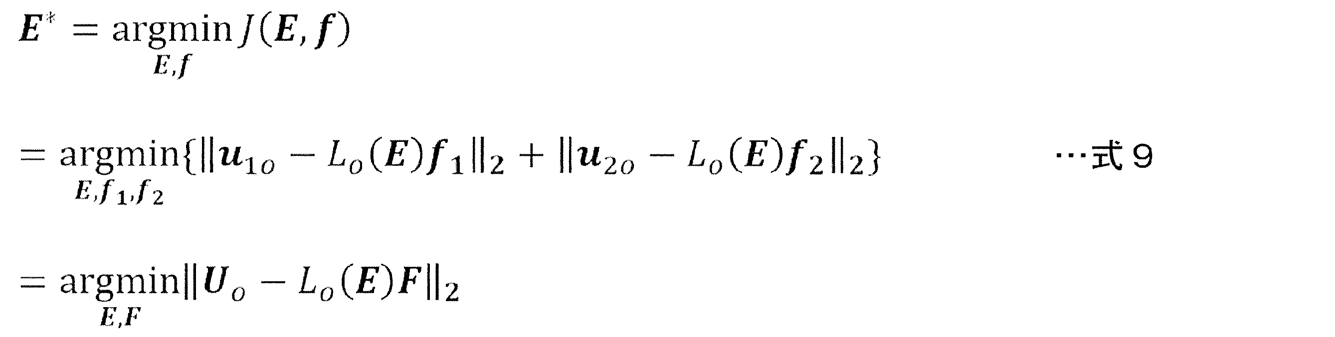 ここで、U0はu1oとu2oを列方向に並べた行列であり、Fはf1とf2を列方向に並べた行列である。また、3行目の式における2次元のノルムは行列のノルムであり、例えばフロベニアスノルムなどである。
図13は、弾性率Eの分布の推定に用いたパターンが1組(実施の形態1)の場合と、パターンが2組(実施の形態2)の場合の実験結果を示す図である。図13の縦軸は真の弾性率Eと推定された弾性率E’との平均二乗誤差(Root Mean Square Error: RMSE)であり、横軸は観察できる頂点数の割合(図9参照)である。
図13からも分かるように、弾性率Eの分布の推定に使用する作用点Paと外力Fの大きさfとで規定される組数が「2」の場合には、実施の形態1の場合(組数が「1」の場合)に比して、観察できる部分の割合が同じであっても、推定精度を高めることができる。
図13からも分かるように、弾性率Eの分布の推定に使用する作用点Paと外力Fの大きさfとで規定される組数が「2」の場合には、実施の形態1の場合(組数が「1」の場合)に比して、観察できる部分の割合が同じであっても、推定精度を高めることができる。
なお、本実施の形態では作点Paと外力Fの大きさfとで規定される組数を「2」としているが、組数は3以上でもよい。一般的に組数が増えるほど推定精度を高めることができる。例えば超音波などの振動を加えることによって評価対象物(例えば臓器)に生じるひずみ像を非侵襲的に評価するための手法の一例であるエラストグラフィ法では、評価対象物に作用させる外力Fが時間的に変化する。すなわち、エラストグラフィ法では、作用点Paと外力Fの大きさfとで規定される組数が複数である。従って、本実施の形態は、エラストグラフィ法との相性がよく、高い精度での推定が可能である。
<実施の形態3>
本実施の形態でも、前述した実施の形態1に比して、弾性率Eの分布の推定精度を高めるための他の手法について説明する。
ここでは、弾性率Eの変化にスパース性を推定できる場合について説明する。スパース性があるとは、要素の大部分が0(ゼロ)を持つという性質のことである。具体的には、一部分だけが硬い又は柔らかいといった局在性があることが知られている弾性体1に適用できる手法である。例えば臓器は、健常組織の弾性率Eは均一であるのに対し、一部の腫瘍部位だけは健常組織に比して硬い(弾性率Eが高い)ことが想定される。従って、臓器の弾性率Eの分布の推定にはスパース性を利用することができる。
本実施の形態でも、前述した実施の形態1に比して、弾性率Eの分布の推定精度を高めるための他の手法について説明する。
ここでは、弾性率Eの変化にスパース性を推定できる場合について説明する。スパース性があるとは、要素の大部分が0(ゼロ)を持つという性質のことである。具体的には、一部分だけが硬い又は柔らかいといった局在性があることが知られている弾性体1に適用できる手法である。例えば臓器は、健常組織の弾性率Eは均一であるのに対し、一部の腫瘍部位だけは健常組織に比して硬い(弾性率Eが高い)ことが想定される。従って、臓器の弾性率Eの分布の推定にはスパース性を利用することができる。
最適化問題に弾性率Eの変化にスパース項を導入することにより、弾性率Eの推定値の変化が局所的であるという制約を与えることができ、その分、推定精度の向上が期待できる。
本実施の形態の場合は、最適化部115は、次式(式10)を満たす未知パラメータを最適解として求める。

本実施の形態の場合は、最適化部115は、次式(式10)を満たす未知パラメータを最適解として求める。
式10の第2項がスパース項である。ここで、E0は、ほとんどの頂点に適用される弾性率の基準値である。従って、スパース項は、各頂点について推定された弾性値Eと基準値との差分(すなわちΔE)について1次元のノルムL1を求める式となる。
本実施の形態では、係数λを0.1とした。この式の場合、弾性率Eが基準値と異なる一部の頂点についてのみ差分ΔE(=E-E0)が非0(ゼロ)となり、大部分の頂点においての差分ΔEは0(ゼロ)となる。このスパース項は、推定された弾性率Eの分布の局在性が高い場合にノルムが小さくなる。従って、スパース項のノルムが大きい弾性率Eの分布は評価が低くなる。なお、係数λの値は一例である。
本実施の形態では、係数λを0.1とした。この式の場合、弾性率Eが基準値と異なる一部の頂点についてのみ差分ΔE(=E-E0)が非0(ゼロ)となり、大部分の頂点においての差分ΔEは0(ゼロ)となる。このスパース項は、推定された弾性率Eの分布の局在性が高い場合にノルムが小さくなる。従って、スパース項のノルムが大きい弾性率Eの分布は評価が低くなる。なお、係数λの値は一例である。
図14は、弾性率Eの分布の推定に用いたパターンが1組(実施の形態1)の場合と、パターンが2組(実施の形態2)の場合と、パターンが2組(実施の形態2)の場合に更に弾性率Eの変化のスパース性を加えた場合(実施の形態3)の実験結果を示す図である。図14の縦軸は真の弾性率Eと推定された弾性率E’との平均二乗誤差(Root Mean Square Error: RMSE)であり、横軸は観察できる頂点数の割合(図9参照)である。
図14からも分かるように、実施の形態2に対して弾性率Eの変化のスパース性を組み合わせた場合には、実施の形態1の場合(組数が「1」の場合)及び実施の形態2の場合(組数が「2」の場合)のいずれに対しても、推定精度を高められることが分かる。特に、実施の形態2に対して弾性率Eの変化のスパース性を組み合わせた場合には、観察できる頂点数の割合が低い場合でも高い推定精度を得ることができる。
図15は、本実施の形態の場合における観測頂点数の割合と観測精度の関係を説明する図である。図15の縦軸は弾性率であり、横軸はブロック番号である。図15は、推定ブロック数Nが40の場合について表している。図では、真の弾性率Eの変化が矩形パルスで表され、推定された弾性率Eの変化が折れ線で表されている。
図15(A)に示すように観測頂点数が全体の49%の場合には2つの波形がおおよそ一致し、図15(B)に示すように観測頂点数が全体の66%の場合には2つの波形の重なり具合が一段と高くなっている。従って、図15が前提とする観測条件の場合には、観察対象である弾性体1の約50%程度を観察できればどの部位が硬いかをおおよそ推定でき(RMSE=0.091907MPa)、約60%以上を観察できればどの部位が硬いかをより高い精度(RMSE=0.024834MPa)で推定できることが分かる。
図15(A)に示すように観測頂点数が全体の49%の場合には2つの波形がおおよそ一致し、図15(B)に示すように観測頂点数が全体の66%の場合には2つの波形の重なり具合が一段と高くなっている。従って、図15が前提とする観測条件の場合には、観察対象である弾性体1の約50%程度を観察できればどの部位が硬いかをおおよそ推定でき(RMSE=0.091907MPa)、約60%以上を観察できればどの部位が硬いかをより高い精度(RMSE=0.024834MPa)で推定できることが分かる。
<他の実施の形態>
前述の実施の形態においては、外力Fの大きさfと弾性率Eの分布がいずれも未知である場合について説明したが、外力Fの大きさfが既知である場合には、未知パラメータの数が減るため、弾性率Eの分布の推定精度を実施の形態1に比して高めることができる。
前述の実施の形態においては、外力Fの大きさfと弾性率Eの分布がいずれも未知である場合について説明したが、外力Fの大きさfが既知である場合には、未知パラメータの数が減るため、弾性率Eの分布の推定精度を実施の形態1に比して高めることができる。
前述した各実施の形態は、様々な用途において活用できる。例えば医師による診断や手術を支援する医療支援システムに情報処理システム100を活用できる他、医療分野以外の産業分野にも、観察や分析の用途にも、生産又は製造の用途にも活用できる。
例えば情報処理システム100を医療支援システムとして活用する場合には、前述したように、視野が限られるために臓器の全体像を一度に観察できなくても、観察できる部位に生じた臓器の変化の情報(観察変位量uo)を用いて、被検体である患者の臓器に固有の弾性率Eの分布を高精度に推定することができる。
前述の実施の形態においては、撮像カメラ20を通じて静止画像を撮像することを前提に説明したが、撮像カメラ20は弾性率Eの推定対象である弾性体1を動画像として撮像できる撮像手段であってもよい。この場合には、撮像された動画像からキャプチャされた静止画像を用いて前述した観察変位量uoを取得してもよい。
また、前述の実施の形態においては、撮像カメラ20が1台である場合について説明したが、撮像カメラ20は複数台あってもよい。また、撮影方向も1つに限らず、複数あってもよい。外力Fによる変形を複数の方向から撮影した画像を用いることによっても観察変位量uoの情報を増やすことができ、推定精度を向上させることができる。
また、前述の実施の形態(例えば実施の形態1)では、推定ブロック数Nが固定値として与えられる場合を前提に説明したが、推定ブロック数Nを増やしながら推定結果の空間分解能を徐々に高める手法を採用してもよい。すなわち、弾性率Eの分布の推定処理を複数ステップに分割してもよい。
例えば初回の推定ステップでは、推定ブロック数Nが10個の場合について推定処理を実行して短時間のうちに推定結果を得て推定結果を表示装置40に表示し、次の推定ステップでは、推定ブロック数Nを予め定めた値(例えば20個)に増加して推定処理の実行と推定結果の表示の更新を繰り返してもよい。このような手法によれば、ユーザは、弾性率Eの分布のおおよそのイメージを早期に把握しつつ、時間の経過につれてより高い空間分解能で取得できる。
例えば初回の推定ステップでは、推定ブロック数Nが10個の場合について推定処理を実行して短時間のうちに推定結果を得て推定結果を表示装置40に表示し、次の推定ステップでは、推定ブロック数Nを予め定めた値(例えば20個)に増加して推定処理の実行と推定結果の表示の更新を繰り返してもよい。このような手法によれば、ユーザは、弾性率Eの分布のおおよそのイメージを早期に把握しつつ、時間の経過につれてより高い空間分解能で取得できる。
以上、本発明の実施の形態について説明したが、本発明の技術的範囲は上記実施の形態に記載の範囲には限定されない。上記実施の形態に、種々の変更又は改良を加えたものも、本発明の技術的範囲に含まれることは、請求の範囲の記載から明らかである。
1…弾性体、10…情報処理装置、100…情報処理システム、111…メッシュモデル生成部、112…観察変位量取得部、113…作用点受付部、114…変位量推定部、115…最適化部、116…表現部、200…メッシュモデル、E…弾性率、F…外力、f…外力の大きさ、uo…観察変位量、uo’…推定変位量、Pa…作用点、Pf…固定点
Claims (14)
- 弾性体の一部分を撮像した画像から取得した観察変位量と当該弾性体の三次元モデルについて算出される推定変位量のうち観察領域に対応する領域部分の推定変位量との差分を最小化する最適解として、既知の作用点に作用する外力の大きさと当該三次元モデルにおける弾性率の分布とを求める演算部
を有する情報処理装置。 - 前記演算部は、次式に基づいて、前記外力の大きさと、前記弾性率の分布を求めることを特徴とする請求項1に記載の情報処理装置。
ここで、
E*は、評価関数J(E,f)を最小にするEとfの集合であり、
Eは、弾性率であり、
E0は、弾性率の基準値であり、
fは、外力の大きさであり、
u0は、観察変位量であり、
L0(E)は、弾性率Eで表現される全体剛性マトリクスKの逆行列成分のうち観察できる部分であり、
L0(E)fは、推定変位量であり、
λは、係数であり、
|| ||1は、1次元のノルムであり、
|| ||2は、2次元のノルムである。 - 弾性体の一部分を撮像した画像から観測変位量を取得する取得部と、
前記弾性体に作用する外力の作用点を受け付ける受付部と、
前記弾性体の三次元モデルにおける弾性率の分布と、前記外力の大きさとを変数として、当該三次元モデルの推定変位量を推定する推定部と、
前記観測変位量と当該観測変位量に対応する前記推定変位量との差分を最小化する最適解として、前記外力の大きさと前記三次元モデルにおける前記弾性率の分布を求める最適化部と
を有する情報処理装置。 - 前記最適化部は、次式に基づいて、前記外力の大きさと、前記弾性率の分布を求めることを特徴とする請求項3に記載の情報処理装置。
ここで、
E*は、評価関数J(E,f)を最小にするEとfの集合であり、
Eは、弾性率であり、
E0は、弾性率の基準値であり、
fは、外力の大きさであり、
u0は、観察変位量であり、
L0(E)は、弾性率Eで表現される全体剛性マトリクスKの逆行列成分のうち観察できる部分であり、
L0(E)fは、推定変位量であり、
λは、係数であり、
|| ||1は、1次元のノルムであり、
|| ||2は、2次元のノルムである。 - 最適解として求められた前記弾性率の分布に基づいて前記三次元モデルを表現する表現部を更に有すること
を特徴とする請求項1又は3に記載の情報処理装置。 - 前記画像は、単一の撮像カメラによって撮像された静止画像であること
を特徴とする請求項1又は3に記載の情報処理装置。 - 前記最適解は、前記弾性率の分布の初期値に対する変化量の絶対値和と前記差分との総和を最小化する値として求められること
を特徴とする請求項1又は3に記載の情報処理装置。 - 前記作用点の情報が複数与えられる場合、前記最適解は、個々の当該作用点について計算される前記差分の総和を最小化する値として求めること
を特徴とする請求項1又は3に記載の情報処理装置。 - 前記作用点に対して複数の前記外力が与えられる場合、前記最適解は、個々の当該外力について計算される前記差分の総和を最小化する値として求めること
を特徴とする請求項1又は3に記載の情報処理装置。 - 前記作用点は複数であり、当該作用点にはそれぞれ異なる前記外力が作用されること
を特徴とする請求項1又は3に記載の情報処理装置。 - 前記最適解を求める空間分解能を低い状態から徐々に高めること
を特徴とする請求項1又は3に記載の情報処理装置。 - 前記作用点に作用する前記外力の大きさが与えられる場合、前記最適解は、前記差分を最小化する前記弾性率の分布として求められること
を特徴とする請求項1又は3に記載の情報処理装置。 - 弾性体の一部分を撮像した画像から観察変位量を取得する処理と、
前記弾性体に作用する外力の作用点を受け付ける処理と、
前記弾性体の三次元モデルにおける弾性率の分布と、前記外力の大きさとを変数として、当該三次元モデルの推定変位量を推定する処理と、
前記観測変位量と当該観測変位量に対応する前記推定変位量との差分を最小化する最適解として、前記外力の大きさと前記三次元モデルにおける前記弾性率の分布を求める処理と
を有する情報処理方法。 - コンピュータに、
弾性体の一部分を撮像した画像から観察変位量を取得する処理と、
前記弾性体に作用する外力の作用点を受け付ける処理と、
前記弾性体の三次元モデルにおける弾性率の分布と、前記外力の大きさとを変数として、当該三次元モデルの推定変位量を推定する処理と、
前記観測変位量と当該観測変位量に対応する前記推定変位量との差分を最小化する最適解として、前記外力の大きさと前記三次元モデルにおける前記弾性率の分布を求める処理と
を実行させるプログラム。
Priority Applications (3)
| Application Number | Priority Date | Filing Date | Title |
|---|---|---|---|
| JP2018559002A JPWO2018123559A1 (ja) | 2016-12-28 | 2017-12-12 | 情報処理装置、情報処理方法及びプログラム |
| US16/474,820 US20200121225A1 (en) | 2016-12-28 | 2017-12-12 | Information processing device, information processing method and program |
| EP17888366.6A EP3564901A4 (en) | 2016-12-28 | 2017-12-12 | INFORMATION PROCESSING DEVICE, INFORMATION PROCESSING PROCESS AND PROGRAM |
Applications Claiming Priority (2)
| Application Number | Priority Date | Filing Date | Title |
|---|---|---|---|
| JP2016-254752 | 2016-12-28 | ||
| JP2016254752 | 2016-12-28 |
Publications (1)
| Publication Number | Publication Date |
|---|---|
| WO2018123559A1 true WO2018123559A1 (ja) | 2018-07-05 |
Family
ID=62707616
Family Applications (1)
| Application Number | Title | Priority Date | Filing Date |
|---|---|---|---|
| PCT/JP2017/044527 Ceased WO2018123559A1 (ja) | 2016-12-28 | 2017-12-12 | 情報処理装置、情報処理方法及びプログラム |
Country Status (4)
| Country | Link |
|---|---|
| US (1) | US20200121225A1 (ja) |
| EP (1) | EP3564901A4 (ja) |
| JP (1) | JPWO2018123559A1 (ja) |
| WO (1) | WO2018123559A1 (ja) |
Citations (2)
| Publication number | Priority date | Publication date | Assignee | Title |
|---|---|---|---|---|
| JP2011177535A (ja) * | 2004-08-24 | 2011-09-15 | General Hospital Corp | 試料の機械的歪み及び弾性的性質を測定するプロセス、システム及びソフトウェア |
| JP2015097724A (ja) * | 2013-11-20 | 2015-05-28 | 株式会社東芝 | 血管解析装置及び血管解析プログラム |
Family Cites Families (1)
| Publication number | Priority date | Publication date | Assignee | Title |
|---|---|---|---|---|
| US9636075B2 (en) * | 2012-08-06 | 2017-05-02 | The University Of North Carolina At Chapel Hill | Simulation-based estimation of elasticity parameters and use of same for non-invasive cancer detection and cancer staging |
-
2017
- 2017-12-12 WO PCT/JP2017/044527 patent/WO2018123559A1/ja not_active Ceased
- 2017-12-12 US US16/474,820 patent/US20200121225A1/en not_active Abandoned
- 2017-12-12 EP EP17888366.6A patent/EP3564901A4/en not_active Withdrawn
- 2017-12-12 JP JP2018559002A patent/JPWO2018123559A1/ja active Pending
Patent Citations (2)
| Publication number | Priority date | Publication date | Assignee | Title |
|---|---|---|---|---|
| JP2011177535A (ja) * | 2004-08-24 | 2011-09-15 | General Hospital Corp | 試料の機械的歪み及び弾性的性質を測定するプロセス、システム及びソフトウェア |
| JP2015097724A (ja) * | 2013-11-20 | 2015-05-28 | 株式会社東芝 | 血管解析装置及び血管解析プログラム |
Non-Patent Citations (2)
| Title |
|---|
| O. GOKSELH. ESKANDARIS. E. SALCUDEAN: "Mesh adaptation for improving elasticity reconstruction using the FEM inverse problem", IEEE TRANS. MED. IMAGING, vol. 32, no. 2, 2013, pages 408 - 418, XP011491229, DOI: doi:10.1109/TMI.2012.2228664 |
| See also references of EP3564901A4 * |
Also Published As
| Publication number | Publication date |
|---|---|
| JPWO2018123559A1 (ja) | 2019-11-07 |
| EP3564901A4 (en) | 2020-08-26 |
| US20200121225A1 (en) | 2020-04-23 |
| EP3564901A1 (en) | 2019-11-06 |
Similar Documents
| Publication | Publication Date | Title |
|---|---|---|
| JP6312898B2 (ja) | 情報処理装置、情報処理方法及びプログラム | |
| Ferrant et al. | Registration of 3D intraoperative MR images of the brain using a finite element biomechanical model | |
| EP1695287B1 (en) | Elastic image registration | |
| US9035941B2 (en) | Image processing apparatus and image processing method | |
| CN104282015B (zh) | 医用图像处理装置以及医用图像处理方法 | |
| De Craene et al. | 3D strain assessment in ultrasound (straus): A synthetic comparison of five tracking methodologies | |
| JP7132299B2 (ja) | 医用画像処理方法、医用画像処理装置、医用画像処理システム及び医用画像処理プログラム | |
| Zhou et al. | A framework for the generation of realistic synthetic cardiac ultrasound and magnetic resonance imaging sequences from the same virtual patients | |
| JP6093347B2 (ja) | 医療画像処理システム及び方法 | |
| CN112967386A (zh) | 生物力学建模方法、装置、电子设备及存储介质 | |
| Visentin et al. | Iterative simulations to estimate the elastic properties from a series of MRI images followed by MRI-US validation | |
| EP2483865A1 (en) | Medical image analysis system for anatomical images subject to deformation and related methods | |
| Plantefeve et al. | Atlas-based transfer of boundary conditions for biomechanical simulation | |
| CN102631196B (zh) | 磁共振弹性成像三维可视化方法及系统 | |
| EP2483866A1 (en) | Medical image analysis system using n-way belief propagation for anatomical images subject to deformation and related methods | |
| EP2483864A1 (en) | Medical image analysis system for displaying anatomical images subject to deformation and related methods | |
| Morita et al. | Model-based estimation of elastic moduli by local displacement observation of an elastic body | |
| Qin et al. | Mapping cardiac fiber orientations from high-resolution DTI to high-frequency 3D ultrasound | |
| KR101227272B1 (ko) | 초음파 영상과 자기공명 영상 간의 영상정합 방법 | |
| JPWO2018131416A1 (ja) | 情報処理装置、情報処理方法及びプログラム | |
| WO2018123559A1 (ja) | 情報処理装置、情報処理方法及びプログラム | |
| Lee et al. | Fast optimization-based elasticity parameter estimation using reduced models | |
| Robert et al. | A generic three-dimensional static force distribution basis for a medical needle inserted into soft tissue | |
| Dahmani et al. | Model-based correction of ultrasound image deformations due to probe pressure | |
| Otani et al. | Assessing cardiac tissue function via action potential wave imaging using cardiac displacement data |
Legal Events
| Date | Code | Title | Description |
|---|---|---|---|
| 121 | Ep: the epo has been informed by wipo that ep was designated in this application |
Ref document number: 17888366 Country of ref document: EP Kind code of ref document: A1 |
|
| WWE | Wipo information: entry into national phase |
Ref document number: 2018559002 Country of ref document: JP |
|
| NENP | Non-entry into the national phase |
Ref country code: DE |
|
| ENP | Entry into the national phase |
Ref document number: 2017888366 Country of ref document: EP Effective date: 20190729 |