WO2022260112A1 - 映像化装置及び映像化方法 - Google Patents
映像化装置及び映像化方法 Download PDFInfo
- Publication number
- WO2022260112A1 WO2022260112A1 PCT/JP2022/023224 JP2022023224W WO2022260112A1 WO 2022260112 A1 WO2022260112 A1 WO 2022260112A1 JP 2022023224 W JP2022023224 W JP 2022023224W WO 2022260112 A1 WO2022260112 A1 WO 2022260112A1
- Authority
- WO
- WIPO (PCT)
- Prior art keywords
- scattering
- function
- information processing
- processing circuit
- measurement data
- Prior art date
- Legal status (The legal status is an assumption and is not a legal conclusion. Google has not performed a legal analysis and makes no representation as to the accuracy of the status listed.)
- Ceased
Links
Images


Classifications
-
- G—PHYSICS
- G01—MEASURING; TESTING
- G01N—INVESTIGATING OR ANALYSING MATERIALS BY DETERMINING THEIR CHEMICAL OR PHYSICAL PROPERTIES
- G01N22/00—Investigating or analysing materials by the use of microwaves or radio waves, i.e. electromagnetic waves with a wavelength of one millimetre or more
-
- G—PHYSICS
- G01—MEASURING; TESTING
- G01B—MEASURING LENGTH, THICKNESS OR SIMILAR LINEAR DIMENSIONS; MEASURING ANGLES; MEASURING AREAS; MEASURING IRREGULARITIES OF SURFACES OR CONTOURS
- G01B15/00—Measuring arrangements characterised by the use of electromagnetic waves or particle radiation, e.g. by the use of microwaves, X-rays, gamma rays or electrons
- G01B15/04—Measuring arrangements characterised by the use of electromagnetic waves or particle radiation, e.g. by the use of microwaves, X-rays, gamma rays or electrons for measuring contours or curvatures
Definitions
- the present disclosure relates to a visualization device or the like that uses waves to visualize the three-dimensional structure of scatterers included in an object within a region.
- Patent Documents 1, 2, 3, 4, and 5 Techniques related to imaging devices that visualize the three-dimensional structure of scatterers contained in objects within a region using waves are disclosed in Patent Documents 1, 2, 3, 4, and 5. I have the technology.
- a beam emitted from a microwave emitter is incident on an inspection object, and the amplitude and phase of the scattered beam are detected by a microwave detector. Then, the distribution of permittivity is calculated from the output signal of the microwave detector, and a tomographic image of the inspection object is displayed.
- the present disclosure provides a visualization device or the like that can visualize, with high accuracy, the three-dimensional structure of scatterers contained in an object within a region using waves.
- a visualization device includes a plurality of transmitters arranged on both sides of a region to be measured to transmit waves to the region, and a plurality of transmitters arranged on both sides to receive the waves from the region.
- the receiver, the measurement data obtained by the plurality of transmitters and the plurality of receivers, and the synthesis of a plurality of functions regarding a plurality of primary scatterings constituting multiple scattering, according to the scattering regarding the scattering of the wave an information processing circuit for deriving an imaging function corresponding to the field function and using the imaging function to visualize a three-dimensional structure of scatterers included in the object in the region.
- FIG. 1 is a conceptual diagram showing an example of orders of multiple scattering in an embodiment.
- FIG. 2 is a diagram representing four scattering modes corresponding to four basic solutions of the scattered field equations.
- FIG. 3 is a conceptual diagram relating to the definition of Green's function.
- FIG. 4 is a conceptual diagram showing an application example of the basic solution of the scattered field.
- FIG. 5 is a diagram showing propagation paths of waves.
- FIG. 6 is a conceptual diagram showing an application example of the basic solution of the scattered field for second-order scattering.
- FIG. 7 is a diagram showing four types of scattering models for third-order scattering.
- FIG. 8 is a diagram showing definitions of four types of measurement data.
- FIG. 9 is a block diagram showing the basic configuration of the imaging device according to the embodiment.
- FIG. 9 is a block diagram showing the basic configuration of the imaging device according to the embodiment.
- FIG. 10 is a conceptual diagram showing an example of the relationship between multiple transmitters, multiple receivers, and regions.
- FIG. 11 is a conceptual diagram showing a modification of the relationship between multiple transmitters, multiple receivers, and regions.
- FIG. 12 is a flow chart showing the basic operation of the imaging device according to the embodiment.
- FIG. 13 is a block diagram showing a specific configuration of the imaging device according to the embodiment.
- a visualization device includes a plurality of transmitters arranged on both sides of a region to be measured to transmit waves to the region, and a plurality of transmitters arranged on both sides to receive the waves from the region.
- the receiver, the measurement data obtained by the plurality of transmitters and the plurality of receivers, and the synthesis of a plurality of functions regarding a plurality of primary scatterings constituting multiple scattering, according to the scattering regarding the scattering of the wave an information processing circuit for deriving an imaging function corresponding to the field function and using the imaging function to visualize a three-dimensional structure of scatterers included in the object in the region.
- the imaging device derives an imaging function for visualizing the three-dimensional structure of the scatterer contained in the object in the region, and corresponds to the measurement data and the synthesis of a plurality of functions related to a plurality of primary scatterings. attachment can be applied. Multiple scattering is assumed to be a combination of multiple primary scattering. Therefore, the imaging device can analytically solve the scattering inverse problem, including multiple scattering, according to this correspondence. Therefore, the imaging device can visualize the three-dimensional structure of the scatterers contained in the object within the region with high accuracy.
- the information processing circuit derives the imaging function corresponding to the scattered field function by solving the equation of the scattered field function based on the measurement data, and the scattered field function is
- ⁇ 5 denotes the Laplace operator with respect to x
- c denotes the propagation speed of the wave
- t is the time from transmission to reception of the wave indicate.
- the imaging device visualizes the three-dimensional structure of the scatterer contained in the object within the region with high accuracy according to the scattered field function associated with the scattering phenomenon and the equation satisfied by the scattered field function. be able to.
- the information processing circuit derives an analytical solution of the equation based on the measurement data, derives the imaging function based on the analytical solution, and the analytical solution is
- k x , k y1 and k y2 denote the wavenumbers for x, y 1 and y 2 of the scattered field function
- a(k x , k y1 , k y2 , k) is k x
- k denote the function based on y1 , ky2 and k
- s1 ( kx , ky1 , ky2 ) denote the function based on kx, ky1 and ky2
- s2( kx, ky1 , k y2 ) denotes a function based on k x , k y1 and k y2 .
- the imaging device can visualize, with high accuracy, the three-dimensional structure of the scatterer contained in the object within the region according to the analytical solution of the equation satisfied by the scattering field function associated with the scattering phenomenon. .
- the visualization function is
- the imaging device can visualize the three-dimensional structure of the scatterers contained in the object within the region with high accuracy according to the imaging function appropriately associated with the scattering field function.
- the multiple scattering is expressed using four functions in spectral space corresponding to four fundamental solutions of the equation of the scattered field function, and the relationship between the measurement data and the four functions is expressed by a nonlinear integral
- the information processing circuit derives the four functions from the measurement data according to the nonlinear integral equation, and uses the four functions to derive the imaging function corresponding to the scattered field function. do.
- the imaging device can visualize the three-dimensional structure of the scatterers included in the object within the region with high accuracy according to the relational expression expressing multiple scattering.
- ⁇ ij , ⁇ 11 , ⁇ 12 , ⁇ 21 and ⁇ 22 are the above for the four scattering modes, two forward scattering corresponding to two directions and two back scattering corresponding to two directions.
- the information processing circuit corresponds to the measurement data, the information processing circuit
- the imaging device can visualize the three-dimensional structure of the scatterers contained in the object within the region with high accuracy according to the formula based on the theory of multiple scattering.
- ⁇ ij , ⁇ 11 , ⁇ 12 , ⁇ 21 and ⁇ 22 are the above for the four scattering modes, two forward scattering corresponding to two directions and two back scattering corresponding to two directions.
- the information processing circuit corresponds to the measurement data, the information processing circuit
- the imaging device can visualize the three-dimensional structure of the scatterer contained in the object within the region with high accuracy according to the formula in which the measurement data are appropriately associated based on the theory of multiple scattering. .
- ⁇ ij , ⁇ 11 , ⁇ 12 , ⁇ 21 and ⁇ 22 are the above for the four scattering modes, two forward scattering corresponding to two directions and two back scattering corresponding to two directions.
- the information processing circuit corresponds to the measurement data, the information processing circuit
- ⁇ denotes the delta function
- k xa , k xb , k xc are the variables corresponding to k x
- k ⁇ and k ⁇ 2 is a variable corresponding to k y1
- k ⁇ 3 is a variable corresponding to k y2
- O(a 4 ) is a term corresponding to 4th order or higher scattering
- the information processing circuit is:
- the imaging device can visualize the three-dimensional structure of the scatterer contained in the object within the region with high accuracy according to the formula that concretely expresses the scattering phenomenon based on the theory of multiple scattering. can.
- ⁇ ij , ⁇ 11 , ⁇ 12 , ⁇ 21 and ⁇ 22 are the above for the four scattering modes, two forward scattering corresponding to two directions and two back scattering corresponding to two directions.
- the information processing circuit corresponds to the measurement data, the information processing circuit
- ⁇ denotes the delta function
- k xa , k xb , k xc are the variables corresponding to k x
- k ⁇ and k ⁇ 2 is a variable corresponding to k y1
- k ⁇ 3 is a variable corresponding to k y2
- the information processing circuit :
- the imaging device can express the scattering phenomenon concretely based on the theory of multiple scattering, and according to the equation in which the measurement data are appropriately associated, the three scattering objects contained in the object within the area can be visualized. Dimensional structures can be visualized with high accuracy.
- ⁇ ij , ⁇ 11 , ⁇ 12 , ⁇ 21 and ⁇ 22 are the above for the four scattering modes, two forward scattering corresponding to two directions and two back scattering corresponding to two directions.
- the information processing circuit corresponds to the measurement data, the information processing circuit
- ⁇ denotes the delta function
- k xa , k xb , k xc are the variables corresponding to k x
- k ⁇ and k ⁇ 2 is a variable corresponding to k y1
- k ⁇ 3 is a variable corresponding to k y2
- the information processing circuit :
- the imaging device can visualize the three-dimensional structure of the scatterers contained in the object within the region with high accuracy according to the formula arranged based on the theory of multiple scattering.
- a visualization method includes a step of transmitting waves to a region to be measured by a plurality of transmitters arranged on both sides of the region; receiving the waves from the region by a receiver; measuring data obtained by the plurality of transmitters and the plurality of receivers; and synthesizing a plurality of functions related to a plurality of primary scatterings constituting multiple scattering. deriving a visualization function corresponding to the scattering field function for scattering of the wave according to the correspondence, and using the visualization function to visualize the three-dimensional structure of scatterers contained in objects in the region. .
- the imaging apparatus uses waves to visualize the three-dimensional structure of scatterers included in objects within a region.
- the imaging apparatus according to the present embodiment will be described in detail, including its underlying technology and theory.
- Scattered field theory has been constructed to visualize the inside of an object using waves such as microwaves. Scattered field theory is not only theoretically novel, but also useful in practice. Since it is possible to instantaneously calculate an accurate three-dimensional reconstructed image from measurement (measurement) data, it is expected to be applied to the field of image diagnosis and the like.
- scattered field theory is developed to solve the difficult problem of inverse scattering of multiple scattering (multiple reflections), and an imaging apparatus and imaging method using the developed scattered field theory are presented.
- a function ⁇ is defined as in the following equation (1-1).
- (x, y 1 , z 1 ) indicate the coordinates of the wave radiating point, and (x, y 2 , z 2 ) indicate the coordinates of the wave receiving point.
- Radiation is sometimes referred to as transmission.
- k indicates the wave number of the wave.
- D indicates the area to be measured.
- .epsilon.(.xi., .eta., .zeta.) denotes a function of the permittivity at the position (.xi., .eta., .zeta.) and corresponds to the wave reflectivity at the position (.xi., .eta., .zeta.).
- ( ⁇ , ⁇ , ⁇ ) correspond to the reflection point of the wave.
- ⁇ 1 indicates the distance from the transmitting point to the reflecting point
- ⁇ 2 indicates the distance from the reflecting point to the receiving point. Note that ⁇ ( ⁇ , ⁇ , ⁇ ) is unknown.
- a phenomenon in which waves are scattered where the value of the dielectric constant function ⁇ ( ⁇ , ⁇ , ⁇ ) is large can be captured as a function of the wave radiating point and receiving point. Then, by defining the emitting point and the receiving point in the entire area, the above ⁇ is used as the scattered field function indicating the scattered field.
- the scattered field function satisfies a partial differential equation such as the following equation (1-2).
- ⁇ 5 denotes the five-dimensional Laplace operator with respect to x, y 1 , y 2 , z 1 and z 2 .
- ⁇ denotes the partial derivative of the variable indicated by the suffix.
- c indicates the wave propagation velocity.
- t indicates time.
- the general solution of the differential equation of formula (1-2) is expressed as in the following formula (1-3).
- k x , k y1 and k y2 denote the wavenumbers for x, y 1 and y 2 of the scattered field function. Since the solution of one fourth-order PDE is completely determined by the measurements (radar return data) at the boundary of the domain, the kernel functions of this general solution, a(k x , k y1 , k y2 , k) is also obtained by Fourier transform.
- the imaging function ⁇ is then obtained by applying the limits of y 2 ⁇ y 1 and t ⁇ 0 to ⁇ . For example, the imaging function ⁇ is expressed by the following equation (1-4).
- the scattered field function ⁇ (x, y 1 , y 2 , z 1 , z 2 , k) is the measured value (radar reflection data).
- Data obtained by Fourier transforming the radar reflection data measured at the interface with respect to (x, t) is expressed as ⁇ (k x , y I , y J , k). Assuming that there is no multiple scattering, the following equation (1-5) is assumed to hold.
- FIG. 1 is a conceptual diagram showing an example of orders of multiple scattering (multiple reflection) in the embodiment.
- P1 indicates a transmission point and P2 indicates a reception point.
- a signal is transmitted from P1 and received at P2 via a number of reflections corresponding to the order in the region. Multiple reflections are called multiple reflections or multiple scattering.
- This disclosure describes a method for solving the inverse scattering problem including multiple scattering as described above, and an imaging apparatus and imaging method using the method.
- Second-order or higher-order multiple scattering is represented by a combination (synthesis) of four basic solutions E 1 , E 2 , E 3 , and E 4 of the partial differential equation of the scattered field.
- FIG. 2 is a diagram representing four scattering modes corresponding to four basic solutions of the scattered field equations. Scattering morphology can also be expressed as a scattering model. Multiple scattering is represented by a composition of these four basic solutions (E 1 , E 2 , E 3 , E 4 ). The spectral space functions a 1 , a 2 , a 3 and a 4 are introduced corresponding to E 1 , E 2 , E 3 and E 4 . To determine these from the measurement data, two backscatter and forward scatter measurements are made.
- ⁇ is an unknown function that indicates the displacement of the vibration at the (x, y, z) position.
- ⁇ 3 denotes the three-dimensional Laplacian operator.
- k indicates a wavenumber. ( ⁇ , ⁇ , ⁇ ) indicates the position of the wave source.
- Equation (2-1) is transformed into equations (2-3) and (2-4).
- ⁇ z 2 denotes the second partial derivative with respect to z.
- a(kx, ky , k ) is a function on (kx, ky , k ).
- This integral kernel function gives the signal strength of a wave leaving r 1 and reflecting at point ⁇ and returning to point r 2 .
- ⁇ is the angular frequency.
- This Green's function is instantiated using a new function name as in the following equation (2-6). where ⁇ is a function of dielectric constant.
- equation (2-7) is considered.
- equation (2-8) is obtained by performing multiple Fourier transform on ⁇ with respect to t, x, y 1 , and y 2 to transform equation (2-7).
- D z1 and D z2 denote partial derivatives with respect to z 1 and z 2 respectively.
- Formula (2-8) has four solutions, which are expressed as in the following formula (2-9).
- s 1 and s 2 are expressed as in the following equation (2-10).
- Equation (2-11) The scattering corresponding to the four basic solutions of equations (2-9) are shown in FIG. Of these four basic solutions, E3 and E4 have a temporal retrograde relationship with each other and are not independent. Therefore, E 1 , E 2 , E 3 are independent elementary solutions.
- Equation (2-7) Four general solutions of Equation (2-7) corresponding to four basic solutions are expressed as in Equation (2-11) below.
- FIG. 4 is a conceptual diagram showing an application example of the basic solution of the scattered field. Specifically, FIG. 4 shows a 3rd order scattering model to which multiple fundamental solutions are applied. For example, in the 3rd order scattering model shown in FIG . 4 , the fundamental solutions E1 and E2 of the scattered field are used in the region inside the dashed line, respectively.
- the following equation (3-1) shows the relationship between the path and the basic solution.
- the scattered points S 1 , S 2 , S 3 are arbitrary points in the region, but the condition that the geometrical rules are observed is imposed on the scattered points S 1 , S 2 , S 3 , etc. Specifically, the sign of the z-coordinate component of the directional vector indicated by the arrow representing wave propagation in FIG. 4 is maintained. Furthermore, P 1 , P 2 , S 2 and S 3 move within the measurement plane under the condition that their x-coordinates are equal to each other. Also, P1 and P2 have the same z - coordinate. However, no constraint on the x - coordinate is assumed for S1.
- FIG. 5 is a diagram showing propagation paths of waves. Specifically, FIG. 5 shows multiple propagation paths for a common transmitting point P 1 and a common receiving point P 2 when basic solutions E 1 and E 2 are used. These multiple propagation paths correspond to the above geometric rules.
- the backscatter amplitude measured on the y-axis is expressed by the following formula (3-2).
- G (specifically, G 1 and G 2 ) is Green's function and is defined by the following equation (3-3).
- Equation (2-11) a 1 (k x , k y1 , k y2 , k) in equation (2-11) is obtained from this equation by Fourier transform.
- G 1 (P 1 , P 2 , k) in which multiple scattering is taken into account is obtained, and a more accurate a 1 (k x , k y1 , k y2 , k) is obtained.
- Equation (3-2) includes a new function G 2 (S 2 ⁇ , S 3 ⁇ , k).
- G 2 the measurement result on a plane with a z value different from that described above is used.
- ⁇ 2 (P 1 , P 2 , k) indicates measurement results on planes with different values of z
- equation (3-5) holds.
- FIG. 6 is a conceptual diagram showing an application example of the basic solution of the scattered field regarding second order scattering.
- Second-order scattering corresponds to the form in which the fundamental solutions E 1 and E 4 of the scattered field equation are connected by S 2 ⁇ as shown in FIG. S 2 ⁇ is assumed to be infinitely close to S 2 .
- the basic solutions E 3 and E 4 satisfy the condition that no direct wave propagating directly from S 2 ⁇ to P 2 is included.
- Equation (3-10) denotes the delta function.
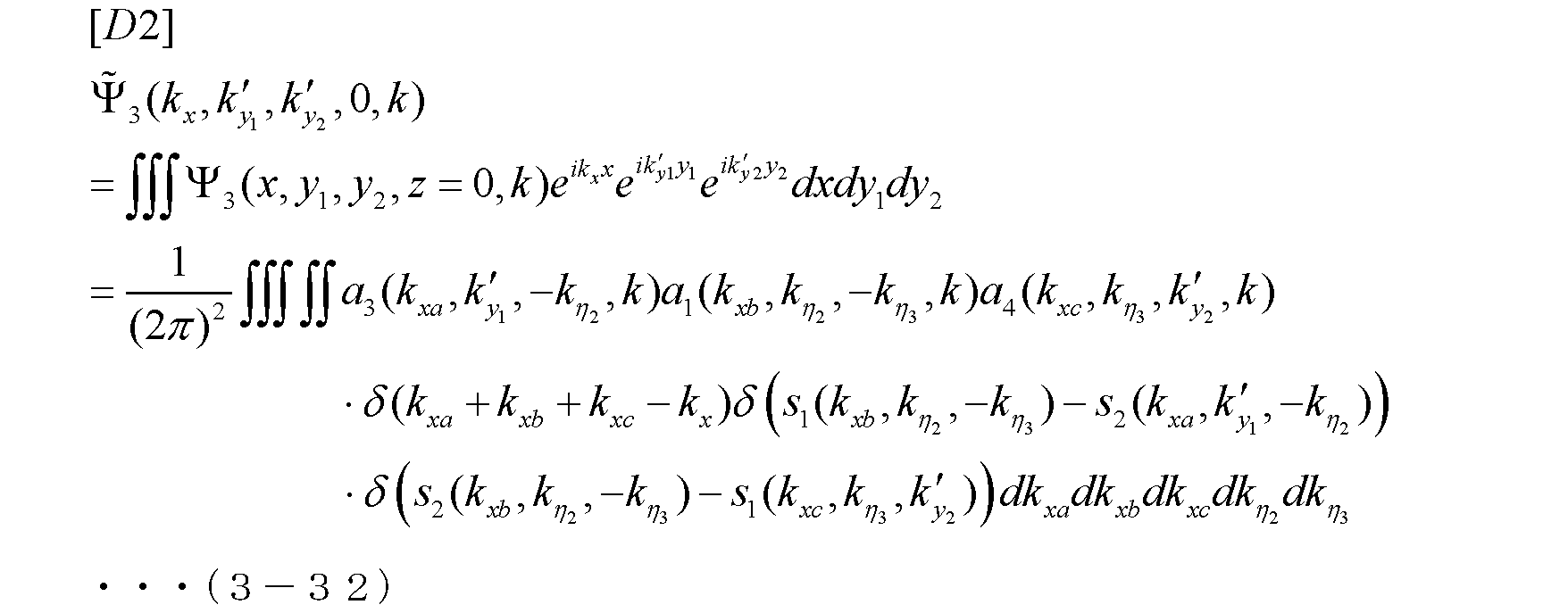
- ⁇ (k ⁇ +k ⁇ + ) and ⁇ (s2(k xa , k y1 , k ⁇ ) ⁇ s1(k xb , k ⁇ + , k y2 )) in equation (3-10) are the connection point S 2 ⁇ corresponds to matching the input and the output in .
- the following equation (3-11) is obtained by Fourier transforming equation (3-10) with respect to (x, y 1 , y 2 ).
- Equation (3-12) corresponds to the general solution of the scattered field of primary scattering, and is a function like the following equation (3-13).
- Equation (3-16) The function obtained by the above process shows the 3rd order scattering amplitudes seen from P 1 , P 2 .
- Equation (3-16) is obtained by substituting equation (3-13) into equation (3-15).
- + and - are appropriately added to the suffix of the wavenumber k to avoid confusion of integral symbols.
- Equation (3-18) is obtained by performing integration on ⁇ and ⁇ in equation (3-16).
- Equation (3-19) denotes the delta function and corresponds to matching of input and output at the junction.
- the scattered field function ⁇ (x, y 1 , y 2 , z, k) is expressed as the following equation (3-20) when multiple scattering is considered.
- equation (3-22) can be obtained by Fourier transforming the entire equation (3-20).
- Equation (3-23) is measurement data on the boundary surface. Therefore, the left side of equation (3-22) is determined. Equation (3-22) is therefore the usual nonlinear integral equation for a 1 (k x , k y1 , k y2 , k) and a 2 (k x , k y1 , k y2 , k).
- FIG. 7 is a diagram showing four types of scattering models for third-order scattering. Specifically, D1, D2, D3 and D4 in FIG. 7 correspond to four types of scattering models for third order scattering. A scattering model can also be expressed as a scattering diagram. In FIG. 7, the regions to which the basic solutions E 1 to E 4 are applied are indicated by dashed lines. The following equations (3-24), (3-25), (3-26), (3-27) and (3-28) represent scattered field functions of D1 to D4.
- ( ⁇ 2- , ⁇ 2- ) and ( ⁇ 3- , ⁇ 3- ) represent the coordinates of points immediately before point S 2 and point S 3 , respectively.
- this equation (3-37) becomes a 1 (k x , k y1 , k y2 , k), a 2 (k x , k y1 , k y2 , k), a 3 (k x , k y1 , k y2 , k) and a 4 (k x , k y1 , k y2 , k).
- FIG. 8 is a diagram showing definitions of four types of measurement data. That is, four types of measurement data for multistatic scattering tomography are defined as shown in FIG. The following equation (3-38) holds from equations (3-31), (3-32), (3-33) and (3-34).
- Equation (3-38) The right sides of the four equations in Equation (3-38) represent four types of functions obtained by Fourier transforming four types of scattered field functions of multiple scattering corresponding to four types of measurement methods.
- Equation (3-37) gives a 1 (k x , k y1 , k y2 , k) when multiple scattering is not considered.
- solutions for which multiple scattering is not considered are marked with the suffix “0”.
- a result like the following equation (3-39) is obtained corresponding to the four types of measurement data in FIG.
- Equation (3-40) is obtained by expanding a 1 , a 2 , a 3 and a 4 into a series corresponding to the order of scattering. Note that a 1 , a 2 , a 3 and a 4 are suffixed with the order of scattering.
- Equation (3-41) is obtained by substituting the measurement data expressed by equation (3-38) into equation (3-37).
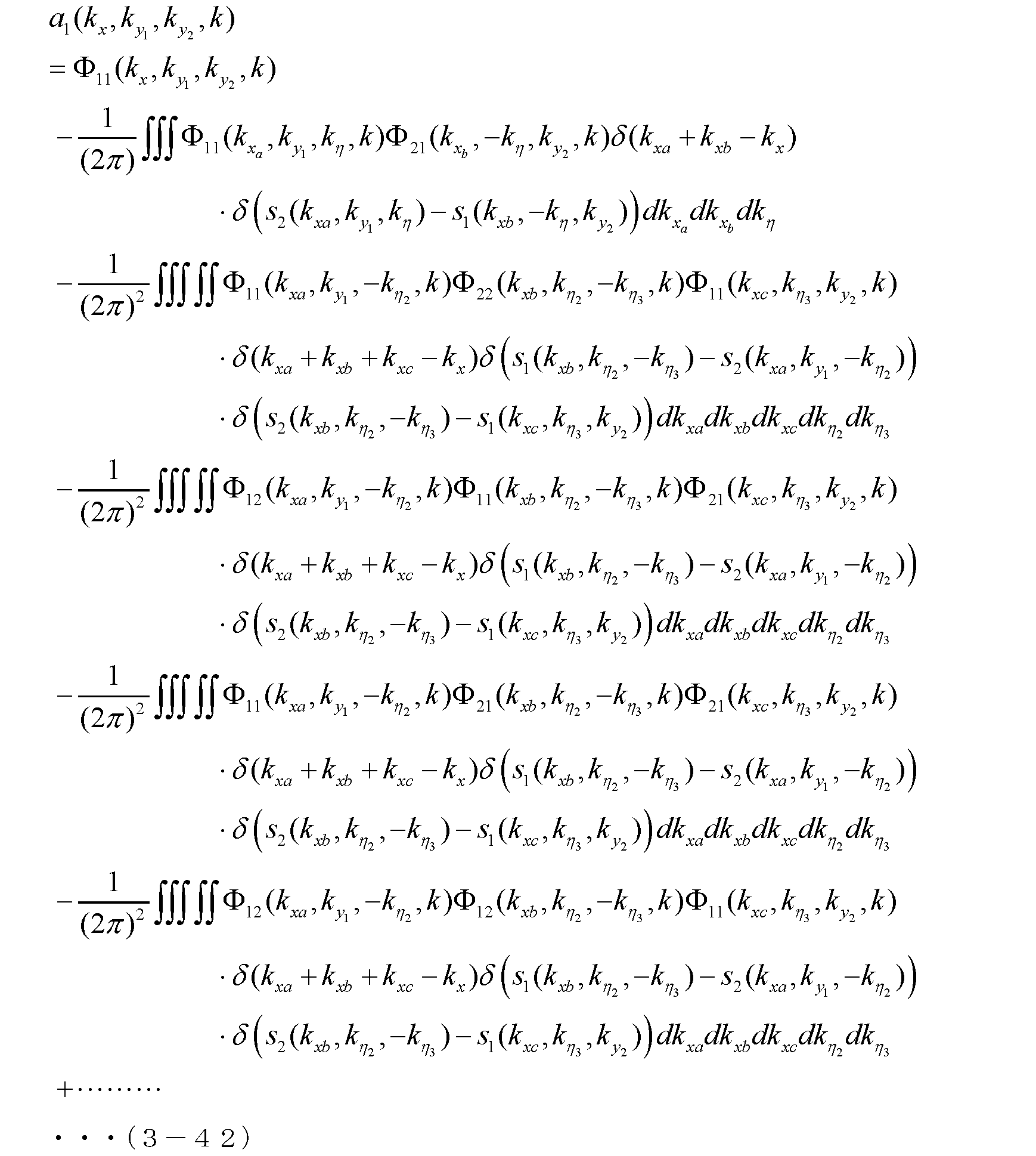
- Equation (3-42) is obtained by substituting equation (3-40) into equation (3-41) and leaving only the 0th order term in the integral symbol.
- a 1 in equation (3-43) corresponds to first, second and third order scattering.
- a1 is derived by removing the effects of secondary scattering and tertiary scattering from the measurement data.
- a 1 corresponding to higher order scattering may be derived in a similar manner.
- a 2 , a 3 and a 4 can be derived by a similar procedure.
- a general solution of the scattered field equation is expressed by the following equation (3-44) using a1.
- the imaging function ⁇ (x, y, z) is expressed by the following equation (3-45) using ⁇ 1 in the above equation (3-44).
- This imaging function is a function from which the influence of multiple scattering has been removed, and is a function that explicitly solves the inverse problem of scattering in the nonlinear case.
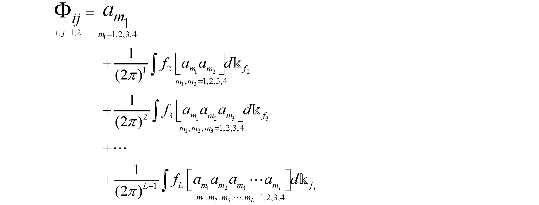
- Formula (3-41) may be generalized as in Formula (3-46) below. Equation (3-46) may then be used as equation (3-41).
- f 2 , f 3 , . . . , f L are 2, 3, . indicates the product of the variables of .
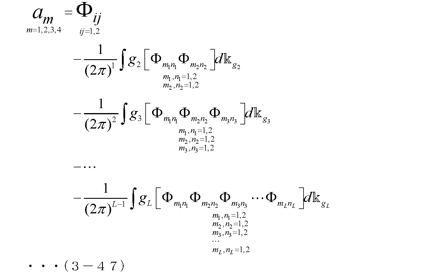
- Equation (3-42) may be generalized as the following formula (3-47). Equation (3-47) may then be used as equation (3-42).
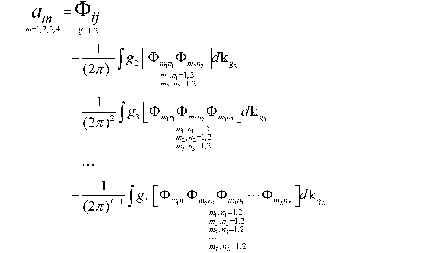
- a 1 , a 2 , a 3 and a 4 represented by am correspond to the analytical solution a( k x , ky1 , ky2 , k) for the four scattering forms.
- ⁇ 11 , ⁇ 12 , ⁇ 21 and ⁇ 22 represented by ⁇ m1n1 , ⁇ m2n2 , ⁇ m3n3 , .
- g 2 , g 3 , . , 3, . . . the product of L variables.
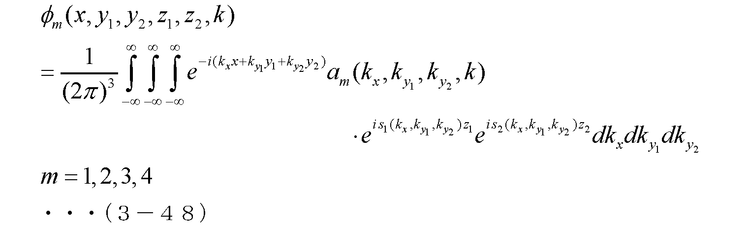
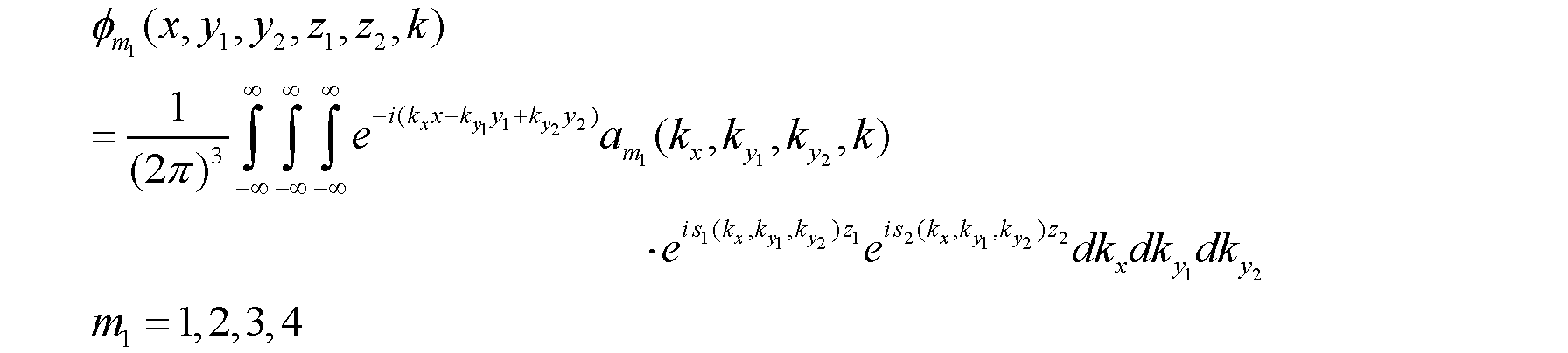
- the scattered field function may be generalized as shown in Equation (3-48) below.
- the imaging function may be generalized as shown in Equation (3-49) below.
- the waves are, for example, radio waves, and may be microwaves, millimeter waves, terahertz waves, or the like. Also, light, sound, or the like may be used as the wave motion. Objects in the area may be living organisms, manufactured products, natural materials, or the like. In particular, the imaging device may be used for mammography and the object may be a breast.
- the scatterers included in the object within the region correspond to portions having physical properties different from those of the surrounding medium.
- this physical property is a physical property corresponding to wave reflectance. If radio waves are used as waves, the physical property may be dielectric constant. Scatterers included in the object may be reinforcing bars included in reinforced concrete, tumors included in the breast, or the like. Also, the area to be measured may be equivalent to the area of the object.
- FIG. 9 is a basic configuration diagram of a visualization device according to this embodiment.
- the imaging device 100 shown in FIG. 9 includes multiple transmitters 101 , multiple receivers 102 and an information processing circuit 103 .
- the imaging device 100 may also include a display 104 .
- Each of the plurality of transmitters 101 is a circuit that transmits waves. Specifically, the plurality of transmitters 101 sequentially transmit waves. A plurality of transmitters 101 are arranged on both sides of the area to be measured.
- Each of the plurality of receivers 102 is a circuit that receives waves. Multiple receivers 102 may simultaneously receive waves in parallel. A plurality of receivers 102, like the plurality of transmitters 101, are arranged on both sides of the area to be measured. Also, the plurality of receivers 102 may be arranged at substantially the same positions as the plurality of transmitters 101 , or may be arranged at different positions from the plurality of transmitters 101 .
- the transmitter 101 and the receiver 102 may configure a multistatic antenna or may configure a monostatic antenna.
- the information processing circuit 103 is a circuit that performs information processing. Specifically, the information processing circuit 103 visualizes the three-dimensional structure of the scatterers included in the object within the region based on the measurement data obtained by the plurality of transmitters 101 and the plurality of receivers 102 . For example, when the information processing circuit 103 visualizes the three-dimensional structure of the scatterer based on the measurement data, the information processing circuit 103 performs arithmetic processing shown in the theory described above.
- the information processing circuit 103 may be a computer or a processor of a computer.
- the information processing circuit 103 may perform information processing by reading a program from memory and executing the program.
- the information processing circuit 103 may be a dedicated circuit that visualizes the three-dimensional structure of the scatterers based on the measurement data.
- the information processing circuit 103 may generate an image showing the three-dimensional structure of the scatterer in order to visualize the three-dimensional structure of the scatterer.
- the information processing circuit 103 may visualize the three-dimensional structure of the scatterer by outputting an image showing the three-dimensional structure of the scatterer to the display 104 or the like. Alternatively, the information processing circuit 103 may visualize the three-dimensional structure of the scatterer by outputting an image showing the three-dimensional structure of the scatterer to a printer (not shown). Alternatively, the information processing circuit 103 may visualize the three-dimensional structure of the scatterer by transmitting the image as electronic data to another device (not shown) through wired or wireless communication.
- the display 104 is a display device such as a liquid crystal display. Note that the display 104 is an optional component and not an essential component. Also, the display 104 may be an external device that does not constitute the imaging device 100 .
- FIG. 10 is a conceptual diagram showing an example of the relationship between multiple transmitters 101, multiple receivers 102, and regions.
- a plurality of transmitters 101 are arranged on both sides of the area to be measured.
- multiple receivers 102 are placed on either side of the area to be measured.
- the plurality of transmitters 101 and the plurality of receivers 102 may be arranged two-dimensionally on each of the two measurement planes.
- transmission and reception may be performed at a plurality of transmission positions and a plurality of reception positions by moving the transmitter 101 and the receiver 102 placed on each of the two measurement planes.
- FIG. 11 is a conceptual diagram showing a modification of the relationship between multiple transmitters 101, multiple receivers 102, and regions. As shown in FIG. 11, multiple transmitters 101 and multiple receivers 102 may be arranged on a curved surface on each side of the area.
- FIG. 12 is a flow chart showing the basic operation of the imaging device 100 shown in FIG. Specifically, the plurality of transmitters 101, the plurality of receivers 102 and the information processing circuit 103 of the imaging apparatus 100 shown in FIG. 9 perform the operations shown in FIG.
- a plurality of transmitters 101 transmit waves to a measurement target area (S101). For example, multiple transmitters 101 transmit waves in sequence. Also, the plurality of receivers 102 receive waves from the measurement target area (S102). For example, multiple receivers 102 receive waves in parallel. Received waves may also be described as scattered waves. Then, the information processing circuit 103 visualizes the three-dimensional structure of the scatterers included in the object within the area using the measurement data obtained by the plurality of transmitters 101 and the plurality of receivers 102 (S103).
- the information processing circuit 103 generates an imaging function corresponding to the scattering field function related to the wave scattering according to the correspondence between the measurement data and the synthesis of the multiple functions related to the multiple primary scattering constituting the multiple scattering. to derive Then, the information processing circuit 103 visualizes the three-dimensional structure of the scatterer included in the object within the area using the imaging function.
- the imaging apparatus 100 derives an imaging function for visualizing the three-dimensional structure of a scatterer contained in an object within an area by combining measurement data with a plurality of functions relating to primary scattering.
- a mapping can be applied. Multiple scattering is assumed to be a combination of multiple primary scattering. Therefore, the imaging device 100 can analytically solve the scattering inverse problem including multiple scattering according to this correspondence. Therefore, the imaging device 100 can visualize the three-dimensional structure of the scatterers included in the object within the region with high accuracy.
- the information processing circuit 103 may derive an imaging function corresponding to the scattered field function by solving the equation of the scattered field function based on the measurement data. Also, the scattered field function is
- (x, y 1 , z 1 ) indicates the wave transmission position
- (x, y 2 , z 2 ) indicates the wave reception position
- k indicates the wave number of the wave
- D is , denote the region
- ( ⁇ , ⁇ , ⁇ ) corresponds to the reflection position of the wave and ⁇ corresponds to the unknown reflectance at the reflection position.
- ⁇ 1 indicates the distance from the transmitting position to the reflecting position
- ⁇ 2 indicates the distance from the reflecting position to the receiving position.
- ⁇ 5 denotes the Laplace operator with respect to x
- c denotes the propagation velocity of the wave
- t denotes the time from transmission to reception of the wave.
- the imaging device 100 visualizes the three-dimensional structure of the scatterer contained in the object in the region with high accuracy according to the scattered field function associated with the scattering phenomenon and the equation satisfied by the scattered field function. can do.
- the information processing circuit 103 may derive an analytical solution of the equation based on the measurement data.
- the information processing circuit 103 may then derive a visualization function based on the analytical solution.
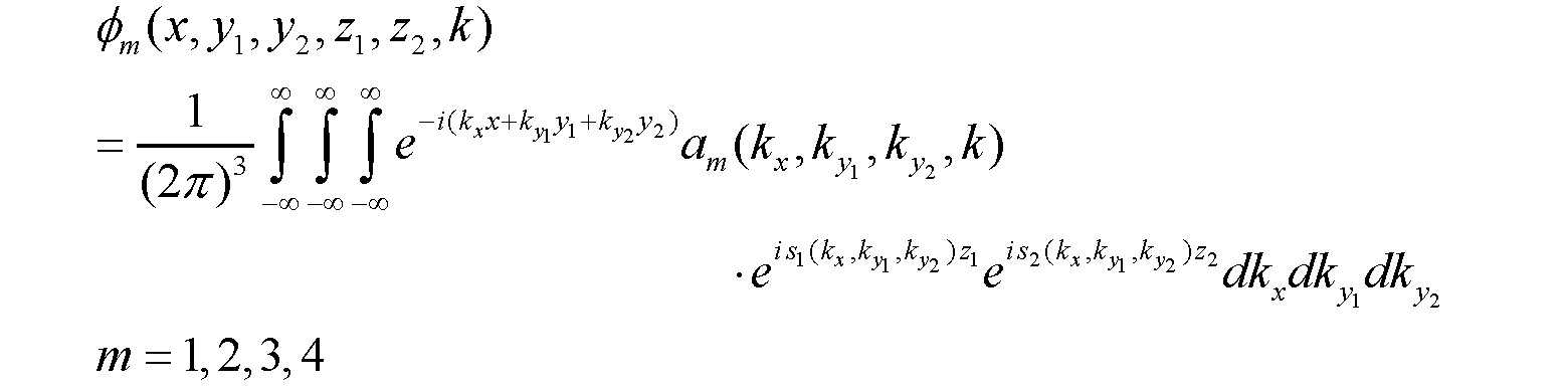
- the analytical solution is
- k x , k y1 and k y2 denote the wavenumbers for x, y 1 and y 2 of the scattered field function.
- a ( kx , ky1, ky2 , k ) denotes a function based on kx, ky1 , ky2 and k
- s1( kx , ky1 , ky2 ) is kx
- Denote the function based on k y1 and k y2 and s 2 (k x , k y1 , k y2 ) denote the function based on k x , k y1 and k y2 .
- the imaging device 100 can visualize with high accuracy the three-dimensional structure of the scatterer contained in the object within the region according to the analytical solution of the equation satisfied by the scattered field function associated with the scattering phenomenon. can.
- the visualization function is
- (x, y, z) indicate the imaging target position.
- the imaging device 100 can visualize the three-dimensional structure of the scatterer included in the object within the region with high accuracy according to the imaging function appropriately associated with the scattering field function.
- multiple scattering may be expressed using four functions in spectral space corresponding to the four fundamental solutions of the equation of the scattered field function.
- the relationship between the measurement data and the four functions may be expressed by a nonlinear integral equation. Then, the information processing circuit 103 may derive four functions from the measurement data according to the nonlinear integral equation. Then, the information processing circuit 103 may derive an imaging function corresponding to the scattered field function using the four functions.
- the imaging device 100 can visualize the three-dimensional structure of the scatterers included in the object within the region with high accuracy according to the relational expression expressing multiple scattering.
- the measurement data For example, the measurement data
- ⁇ 11 , ⁇ 12 , ⁇ 21 and ⁇ 22 represented by ⁇ ij are measurement data on four scattering modes, two forward scattering corresponding to two directions and two back scattering corresponding to two directions. corresponds to
- the imaging device 100 can visualize the three-dimensional structure of the scatterers included in the object within the region with high accuracy according to the formula based on the theory of multiple scattering.
- ⁇ 11 , ⁇ 12 , ⁇ 21 and ⁇ 22 represented by ⁇ ij are measurement data on four scattering modes, two forward scattering corresponding to two directions and two back scattering corresponding to two directions. corresponds to
- a 1 , a 2 , a 3 and a 4 represented by am correspond to the analytical solution a( k x , ky1 , ky2 , k) for the four scattering forms.
- ⁇ 11 , ⁇ 12 , ⁇ 21 and ⁇ 22 represented by ⁇ m1n1 , ⁇ m2n2 , ⁇ m3n3 , .
- g 2 , g 3 , . , 3, . . . the product of L variables.
- the imaging apparatus 100 can visualize the three-dimensional structure of the scatterer included in the object within the region with high accuracy according to the formula in which the measurement data are appropriately associated based on the theory of multiple scattering. can.
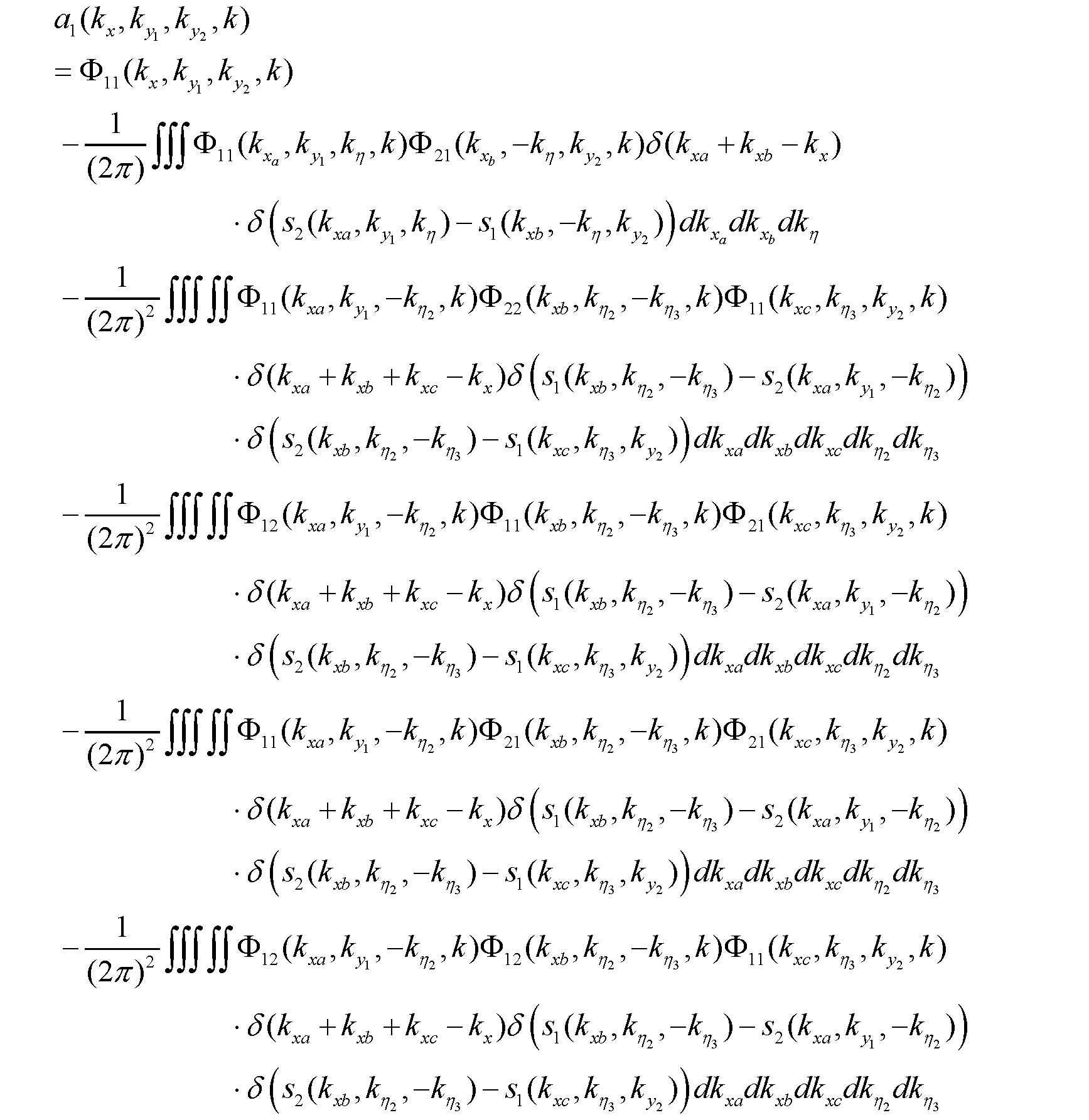
- ⁇ 11 , ⁇ 12 , ⁇ 21 and ⁇ 22 represented by ⁇ ij are measurement data on four scattering modes, two forward scattering corresponding to two directions and two back scattering corresponding to two directions. corresponds to
- ⁇ denotes the delta function
- k xa , k xb , k xc are variables corresponding to k x
- k ⁇ and k ⁇ 2 are variables corresponding to k y1
- k ⁇ 3 is A variable corresponding to k y2
- O(a 4 ) is a term corresponding to fourth-order or higher scattering.
- the imaging device 100 can visualize the three-dimensional structure of the scatterer contained in the object in the region with high accuracy according to the formula specifically expressing the scattering phenomenon based on the theory of multiple scattering. can be done.
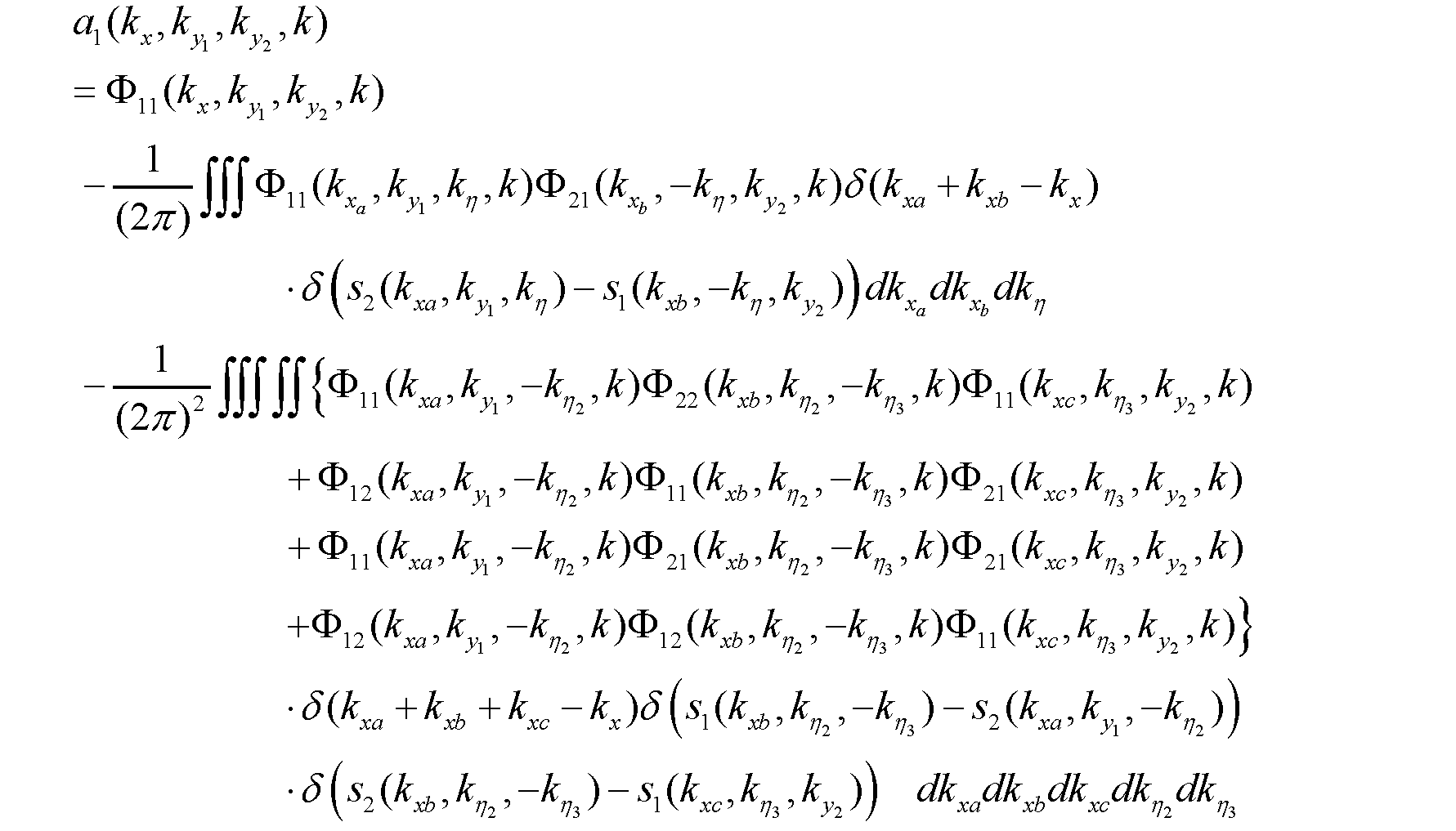
- ⁇ 11 , ⁇ 12 , ⁇ 21 and ⁇ 22 represented by ⁇ ij are measurement data on four scattering modes, two forward scattering corresponding to two directions and two back scattering corresponding to two directions. corresponds to
- ⁇ denotes the delta function
- k xa , k xb , k xc are variables corresponding to k x
- k ⁇ and k ⁇ 2 are variables corresponding to k y1
- k ⁇ 3 is ky is a variable corresponding to y2 .
- the imaging apparatus 100 can express the scattering phenomenon concretely based on the theory of multiple scattering, and according to the equation in which the measurement data are appropriately associated, the scatterer included in the object in the area can be detected. Three-dimensional structures can be visualized with high accuracy.
- ⁇ 11 , ⁇ 12 , ⁇ 21 and ⁇ 22 represented by ⁇ ij are measurement data on four scattering modes, two forward scattering corresponding to two directions and two back scattering corresponding to two directions. corresponds to
- ⁇ denotes the delta function
- k xa , k xb , k xc are variables corresponding to k x
- k ⁇ and k ⁇ 2 are variables corresponding to k y1 , k ⁇ 3 to k y2 is the corresponding variable.
- the imaging device 100 can visualize the three-dimensional structure of the scatterers included in the object within the region with high accuracy according to the formula arranged based on the theory of multiple scattering.
- the scattered field function may be defined as a function in which a wave transmission position and a wave reception position are input and a value indicating the wave at the reception position is output.
- the imaging function may be determined based on values output from the scattered field function by inputting imaging target positions as the transmission position and the reception position into the scattered field function.
- the information processing circuit 103 may derive a scattered field function using the measurement data as a boundary condition, and derive an imaging function using the scattered field function.
- the plurality of transmitters 101, the plurality of receivers 102, the information processing circuit 103, the scattered field function, the imaging function, and the like shown in the basic configuration and basic operation described above may include the functions shown in the present embodiment. Other components, formulas and variables, etc. may be applied as appropriate.
- the scattered field function, the imaging function, and the like shown in the present embodiment may be modified as appropriate and applied.
- a mathematical expression that expresses substantially the same content as the above-described mathematical expression in another expression may be used, or another mathematical expression derived based on the above-described theory may be used.
- FIG. 13 is a block diagram showing a specific configuration of imaging device 100 shown in FIG.
- the transmitter 101 and receiver 102 of the imaging device 100 shown in FIG. 9 may be included in the multi-static array antenna 1008.
- the information processing circuit 103 of the imaging device 100 shown in FIG. 9 may correspond to one or more of the multiple components shown in FIG. Specifically, for example, the information processing circuit 103 may correspond to the signal processing computer 1005 . Also, the display 104 shown in FIG. 9 may correspond to the signal monitoring device 1006 .
- the microwave signal used in the imaging device 100 is a pseudo-random time-series signal (PN code: Pseudo Noise Code) having frequency components of DC to 20 GHz.
- PN code Pseudo Noise Code
- This signal is output from the FPGA board 1002 for PN code generation. More specifically, there are two types of this signal.
- One type of signal (LO signal: local oscillator signal) is sent through the delay circuit (digital control board 1003) to the RF detector circuit (RF detector board 1007).
- the other type of signal (RF signal: Radio Frequency Signal) is sent to the transmitting microwave UWB antenna of the multi-static array antenna 1008 and radiated.
- a scattered microwave signal is received by the receiving UWB antenna of the multi-static array antenna 1008 and sent to the RF detection circuit (RF detection board 1007).
- the transmission/reception signals pass through the antenna element selection switch (UWB antenna RF switch 1004).
- the delayed signal (LO signal) is delayed by 1/ 2n times (n is an integer greater than 2) the time at which the value of the PN code changes.
- the detected signal is A/D converted by the signal processing computer 1005 and stored as an IF signal (Intermediate Frequency Signal). Information indicating the detected signal may also be displayed on the signal monitoring device 1006 .
- the timing of these series of operations is controlled by the microprocessor in the digital control board 1003 so as to synchronize with the signal (distance signal or free run signal) from the rangefinder 1001.
- the microprocessor in the digital control board 1003 sends Switch switching signals, PN code sweep triggers, and the like.
- the signal processing computer 1005 also uses the A/D-converted and stored signals to perform three-dimensional reconstruction and display a three-dimensional image.
- the signal processing calculator 1005 may also perform signal calibration.
- the signal processing computer 1005 may display raw waveforms.
- the signal processing computer 1005 may store a three-dimensional image or the like in the memory 1009 .
- the configuration shown in FIG. 13 is an example, and the configuration of imaging device 100 is not limited to the configuration shown in FIG. A part of the configuration shown in FIG. 13 may be omitted or changed.
- the imaging method including the steps performed by each component of the imaging device may be executed by any device or system.
- part or all of the imaging method may be performed by a computer including a processor, memory, input/output circuitry, and the like.
- the imaging method may be executed by the computer executing a program for causing the computer to execute the imaging method.
- the above program may be recorded on a non-temporary computer-readable recording medium.
- each component of the imaging apparatus may be configured with dedicated hardware, may be configured with general-purpose hardware that executes the above programs, etc., or may be configured with a combination of these. good.
- the general-purpose hardware may be composed of a memory in which a program is recorded, a general-purpose processor that reads and executes the program from the memory, and the like.
- the memory may be a semiconductor memory, a hard disk, or the like, and the general-purpose processor may be a CPU or the like.
- dedicated hardware may be configured with a memory, a dedicated processor, and the like.
- a dedicated processor may refer to a memory for recording measurement data and perform the imaging method described above.
- each component of the imaging device may be an electric circuit.
- These electric circuits may form one electric circuit as a whole, or may be separate electric circuits. Further, these electric circuits may correspond to dedicated hardware, or may correspond to general-purpose hardware for executing the above-described programs and the like.
- One aspect of the present disclosure is useful for an imaging device that uses waves to visualize the three-dimensional structure of scatterers contained in objects within a region, and is applicable to geophysical exploration, medical diagnosis, and the like.
- Imaging Device 101 Transmitter 102 Receiver 103 Information Processing Circuit 104 Display 1001 Rangefinder 1002 FPGA Board for PN Code Generation 1003 Digital Control Board 1004 UWB Antenna RF Switch 1005 Signal Processing Calculator 1006 Signal Monitoring Device 1007 RF Detection Board 1008 Multistatic Array antenna 1009 Memory
Landscapes
- Physics & Mathematics (AREA)
- Electromagnetism (AREA)
- General Physics & Mathematics (AREA)
- General Health & Medical Sciences (AREA)
- Pathology (AREA)
- Chemical & Material Sciences (AREA)
- Analytical Chemistry (AREA)
- Biochemistry (AREA)
- Health & Medical Sciences (AREA)
- Immunology (AREA)
- Life Sciences & Earth Sciences (AREA)
- Analysing Materials By The Use Of Radiation (AREA)
- Radar Systems Or Details Thereof (AREA)
- Image Processing (AREA)
- Investigating Or Analysing Materials By Optical Means (AREA)
- Measurement Of Velocity Or Position Using Acoustic Or Ultrasonic Waves (AREA)
- Image Analysis (AREA)
- Air Bags (AREA)
- Studio Devices (AREA)
Abstract
Description







本実施の形態における映像化装置は、波動を用いて、領域内の物体に含まれる散乱体の3次元構造を可視化する。以下、本実施の形態における映像化装置をその基礎となる技術及び理論なども含めて、詳細に説明する。
マイクロ波等の波動を用いて物体内の映像化を行うために散乱場理論が構築されている。散乱場理論は、単に理論上の新しさを有するだけではなく実用にも役立つ。計測(測定)データから瞬時に正確な3次元再構成画像を計算できるため、画像診断分野等への応用が期待される。本開示では、散乱場理論を多重散乱(多重反射)の逆散乱問題という難問の解決のために発展させ、発展した散乱場理論を用いる映像化装置及び映像化方法が示される。


<II-1 単純な伝搬関数>
波動の伝搬のヘルムホルツ方程式は、次式(2-1)で表現される。


図3は、グリーン関数の定義に関する概念図である。以下断らない限り、送信点と受信点とが同じx座標を有する。送信点及び受信点が、それぞれr1=(x、y1、z1)及びr2=(x、y2、z2)である場合、グリーン関数が次式(2-5)のように定義される。



<III-1 多重散乱の次数>
多重散乱の次数は、図1に示した通りである。図1に示した各次数の多重散乱においても、散乱の起きる場所で様々に異なる幾何学的なバラエティが存在する。そして、散乱の起きる場所での入射及び散乱の各方向ベクトルのz座標成分の正負により、特性が異なる。入射及び散乱の各方向ベクトルのz座標成分の正負により特性が異なることは、II章の散乱場の基本解で説明されている。
図4は、散乱場の基本解の適用例を示す概念図である。具体的には、図4には、複数の基本解が適用される3次の散乱モデルが示されている。例えば、図4に示した3次の散乱モデルでは、散乱場の基本解E1及びE2が、それぞれ、破線内部の領域で用いられる。次式(3-1)は、経路と基本解との関係を示す。


(1)2次の散乱
図6は、2次の散乱に関する散乱場の基本解の適用例を示す概念図である。2次の散乱は、図6に示すように、散乱場の方程式の基本解E1とE4とがS2-で接続された形に対応する。S2-は、限りなくS2に近いと仮定されている。基本解E3、E4では、S2-からP2へ直接伝搬する直接波が含まれないという条件が満たされている。





3次の散乱について散乱場の基本解が適用される例は、図4の通りである。図4を参照して次式(3-12)のような散乱場関数が定義される。η、ζに対するサフィックス2-、3-は、それぞれ、点S2の直前、点S3の直前に対応している。


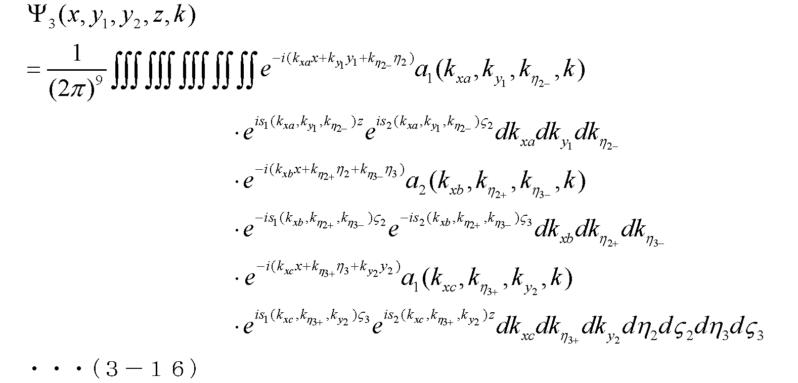



図7は、3次の散乱に関する4種類の散乱モデルを示す図である。具体的には、図7のD1、D2、D3及びD4は、3次の散乱に関する4種類の散乱モデルに対応する。散乱モデルは、散乱のダイヤグラムとも表現され得る。図7において、基本解E1~E4が適用される領域が破線で示されている。以下の式(3-24)、式(3-25)式(3-26)、式(3-27)及び式(3-28)は、D1~D4の散乱場関数を示す。




散乱場関数Ψ(x、y1、y2、z、k)は、多重散乱が考慮される場合、次式(3-35)のように表現される。


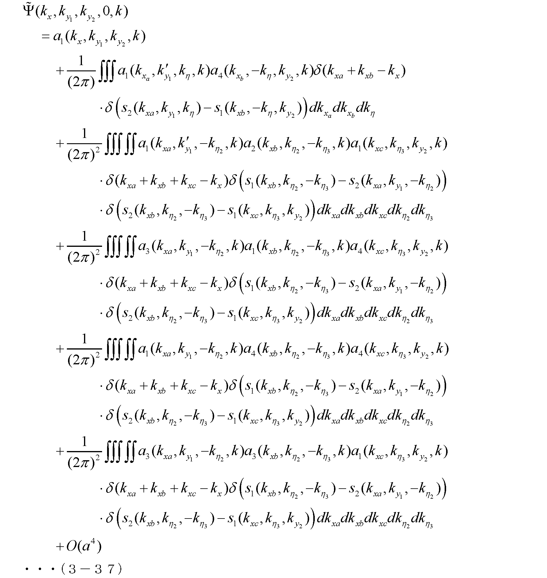

図8は、4種類の計測データの定義を示す図である。つまり、マルチスタティック散乱トモグラフィの4種類の計測データが図8のように定義される。式(3-31)、(3-32)、(3-33)及び(3-34)等から、次式(3-38)が成立する。






上述された内容に基づいて、以下に、波動を用いて領域内の物体に含まれる散乱体の3次元構造を可視化する映像化装置の構成及び動作を示す。















以上、映像化装置の態様を実施の形態に基づいて説明したが、映像化装置の態様は、実施の形態に限定されない。実施の形態に対して当業者が思いつく変形が施されてもよいし、実施の形態における複数の構成要素が任意に組み合わされてもよい。例えば、実施の形態において特定の構成要素によって実行される処理を特定の構成要素の代わりに別の構成要素が実行してもよい。また、複数の処理の順序が変更されてもよいし、複数の処理が並行して実行されてもよい。
101 送信器
102 受信器
103 情報処理回路
104 ディスプレイ
1001 距離計
1002 PN符号生成用FPGAボード
1003 デジタル制御ボード
1004 UWBアンテナRFスイッチ
1005 信号処理計算機
1006 信号モニタ装置
1007 RF検波ボード
1008 マルチスタティックアレイアンテナ
1009 メモリ
Claims (11)
- 計測対象の領域の両側に配置され、前記領域へ波動を送信する複数の送信器と、
前記両側に配置され、前記領域から前記波動を受信する複数の受信器と、
前記複数の送信器及び前記複数の受信器によって得られる計測データと、多重散乱を構成する複数の一次散乱に関する複数の関数の合成との対応付けに従って、前記波動の散乱に関する散乱場関数に対応する映像化関数を導出し、前記映像化関数を用いて前記領域内の物体に含まれる散乱体の3次元構造を可視化する情報処理回路とを備える
映像化装置。 - 前記情報処理回路は、前記散乱場関数の方程式を前記計測データに基づいて解くことにより、前記散乱場関数に対応する前記映像化関数を導出し、
前記散乱場関数は、

前記方程式は、

請求項1に記載の映像化装置。 - 前記情報処理回路は、前記計測データに基づいて前記方程式の解析解を導出し、前記解析解に基づいて前記映像化関数を導出し、
前記解析解は、

請求項2に記載の映像化装置。 - 前記情報処理回路は、前記解析解に基づいて、前記映像化関数を導出し、
前記映像化関数は、

請求項3に記載の映像化装置。 - 前記多重散乱は、前記散乱場関数の方程式の4つの基本解に対応するスペクトル空間の4つの関数を用いて表現され、
前記計測データと前記4つの関数との関係は、非線形積分方程式で表現され、
前記情報処理回路は、
前記計測データから、前記非線形積分方程式に従って、前記4つの関数を導出し、
前記4つの関数を用いて前記散乱場関数に対応する前記映像化関数を導出する
請求項1に記載の映像化装置。 - 前記計測データは、

前記情報処理回路は、


am1、am2、am3、・・・、amLで表現されるa1、a2、a3及びa4は、前記4つの散乱形態に関する前記解析解のa(kx、ky1、ky2、k)に対応し、f2、f3、・・・、fLは、それぞれ、前記波動の送信から受信までに適用される2回、3回、・・・、L回の散乱に対応する括弧内の2個、3個、・・・、L個の変数の積を示し、

前記情報処理回路は、


請求項4に記載の映像化装置。 - 前記計測データは、

前記情報処理回路は、


amで表現されるa1、a2、a3及びa4は、前記4つの散乱形態に関する前記解析解のa(kx、ky1、ky2、k)に対応し、Φm1n1、Φm2n2、Φm3n3、・・・、ΦmLnLで表現されるΦ11、Φ12、Φ21及びΦ22は、前記4つの散乱形態に関する前記計測データに対応し、g2、g3、・・・、gLは、それぞれ、前記波動の送信から受信までに適用される2回、3回、・・・、L回の散乱に対応する括弧内の2個、3個、・・・、L個の変数の積を示し、

前記情報処理回路は、

請求項4に記載の映像化装置。 - 前記計測データは、

前記情報処理回路は、

δは、デルタ関数を示し、kxa、kxb、kxcは、kxに対応する変数であり、kη及びkη2は、ky1に対応する変数であり、kη3は、ky2に対応する変数であり、O(a4)は、4次以上の散乱に対応する項であり、
前記情報処理回路は、


請求項4に記載の映像化装置。 - 前記計測データは、

前記情報処理回路は、

δは、デルタ関数を示し、kxa、kxb、kxcは、kxに対応する変数であり、kη及びkη2は、ky1に対応する変数であり、kη3は、ky2に対応する変数であり、
前記情報処理回路は、


請求項4に記載の映像化装置。 - 前記計測データは、

前記情報処理回路は、

δは、デルタ関数を示し、kxa、kxb、kxcは、kxに対応する変数であり、kη及びkη2は、ky1に対応する変数であり、kη3は、ky2に対応する変数であり、
前記情報処理回路は、


請求項4に記載の映像化装置。 - 計測対象の領域の両側に配置された複数の送信器によって、前記領域へ波動を送信するステップと
前記両側に配置された複数の受信器によって、前記領域から前記波動を受信するステップと、
前記複数の送信器及び前記複数の受信器によって得られる計測データと、多重散乱を構成する複数の一次散乱に関する複数の関数の合成との対応付けに従って、前記波動の散乱に関する散乱場関数に対応する映像化関数を導出し、前記映像化関数を用いて前記領域内の物体に含まれる散乱体の3次元構造を可視化するステップとを含む
映像化方法。
Priority Applications (8)
| Application Number | Priority Date | Filing Date | Title |
|---|---|---|---|
| CA3219990A CA3219990A1 (en) | 2021-06-11 | 2022-06-09 | Imaging device and imaging method |
| AU2022290444A AU2022290444B2 (en) | 2021-06-11 | 2022-06-09 | Imaging device and imaging method |
| KR1020237041547A KR20240019106A (ko) | 2021-06-11 | 2022-06-09 | 영상화 장치 및 영상화 방법 |
| IL308548A IL308548A (en) | 2021-06-11 | 2022-06-09 | Imaging device and imaging method |
| CN202280037553.7A CN117377870A (zh) | 2021-06-11 | 2022-06-09 | 影像化装置以及影像化方法 |
| EP22820291.7A EP4354125A4 (en) | 2021-06-11 | 2022-06-09 | IMAGING DEVICE AND IMAGING METHOD |
| US18/567,141 US20240280361A1 (en) | 2021-06-11 | 2022-06-09 | Imaging device and imaging method |
| JP2023527914A JP7813474B2 (ja) | 2021-06-11 | 2022-06-09 | 映像化装置及び映像化方法 |
Applications Claiming Priority (2)
| Application Number | Priority Date | Filing Date | Title |
|---|---|---|---|
| JP2021-098329 | 2021-06-11 | ||
| JP2021098329 | 2021-06-11 |
Publications (1)
| Publication Number | Publication Date |
|---|---|
| WO2022260112A1 true WO2022260112A1 (ja) | 2022-12-15 |
Family
ID=84425115
Family Applications (1)
| Application Number | Title | Priority Date | Filing Date |
|---|---|---|---|
| PCT/JP2022/023224 Ceased WO2022260112A1 (ja) | 2021-06-11 | 2022-06-09 | 映像化装置及び映像化方法 |
Country Status (9)
| Country | Link |
|---|---|
| US (1) | US20240280361A1 (ja) |
| EP (1) | EP4354125A4 (ja) |
| JP (1) | JP7813474B2 (ja) |
| KR (1) | KR20240019106A (ja) |
| CN (1) | CN117377870A (ja) |
| AU (1) | AU2022290444B2 (ja) |
| CA (1) | CA3219990A1 (ja) |
| IL (1) | IL308548A (ja) |
| WO (1) | WO2022260112A1 (ja) |
Cited By (1)
| Publication number | Priority date | Publication date | Assignee | Title |
|---|---|---|---|---|
| WO2024190178A1 (ja) | 2023-03-10 | 2024-09-19 | 文俊 木村 | 映像化装置及び映像化方法 |
Citations (12)
| Publication number | Priority date | Publication date | Assignee | Title |
|---|---|---|---|---|
| JPS6266145A (ja) | 1985-09-06 | 1987-03-25 | シ−メンス、アクチエンゲゼルシヤフト | 誘電率分布検出方法 |
| JP2000514917A (ja) * | 1996-06-26 | 2000-11-07 | ユニバーシティー オブ ユタ リサーチ ファンデーション | 広帯域電磁ホログラフィック画像化方法 |
| US20040034307A1 (en) * | 1992-10-14 | 2004-02-19 | Johnson Steven A. | Apparatus and method for imaging objects with wavefields |
| WO2014125815A1 (ja) | 2013-02-12 | 2014-08-21 | 国立大学法人神戸大学 | 散乱トモグラフィ方法および散乱トモグラフィ装置 |
| WO2015136936A1 (ja) | 2014-03-12 | 2015-09-17 | 国立大学法人神戸大学 | 散乱トモグラフィ方法および散乱トモグラフィ装置 |
| JP2017509416A (ja) * | 2014-03-31 | 2017-04-06 | コーニンクレッカ フィリップス エヌ ヴェKoninklijke Philips N.V. | 肋骨間空間を用いたコヒーレントな複合による音響撮像のためのシステム及び方法 |
| WO2017057524A1 (ja) * | 2015-09-29 | 2017-04-06 | 国立大学法人神戸大学 | 画像化方法および画像化装置 |
| JP2018512985A (ja) * | 2015-04-01 | 2018-05-24 | ヴェラゾニックス,インコーポレーテッド | インパルス応答推定及び遡及的取得による符号化励起イメージングのための方法及びシステム |
| JP2019510593A (ja) * | 2016-01-18 | 2019-04-18 | メディカル ワイヤレス センシング リミテッド | マイクロ波トモグラフィシステム |
| JP2020031714A (ja) * | 2018-08-27 | 2020-03-05 | 国立大学法人静岡大学 | 診断装置、診断方法、診断プログラム |
| WO2021020387A1 (ja) | 2019-08-01 | 2021-02-04 | 株式会社 Integral Geometry Science | 散乱トモグラフィ装置及び散乱トモグラフィ方法 |
| WO2021053971A1 (ja) | 2019-09-17 | 2021-03-25 | 株式会社 Integral Geometry Science | 散乱トモグラフィ装置及び散乱トモグラフィ方法 |
-
2022
- 2022-06-09 WO PCT/JP2022/023224 patent/WO2022260112A1/ja not_active Ceased
- 2022-06-09 KR KR1020237041547A patent/KR20240019106A/ko active Pending
- 2022-06-09 JP JP2023527914A patent/JP7813474B2/ja active Active
- 2022-06-09 IL IL308548A patent/IL308548A/en unknown
- 2022-06-09 EP EP22820291.7A patent/EP4354125A4/en active Pending
- 2022-06-09 CN CN202280037553.7A patent/CN117377870A/zh active Pending
- 2022-06-09 US US18/567,141 patent/US20240280361A1/en active Pending
- 2022-06-09 AU AU2022290444A patent/AU2022290444B2/en active Active
- 2022-06-09 CA CA3219990A patent/CA3219990A1/en active Pending
Patent Citations (12)
| Publication number | Priority date | Publication date | Assignee | Title |
|---|---|---|---|---|
| JPS6266145A (ja) | 1985-09-06 | 1987-03-25 | シ−メンス、アクチエンゲゼルシヤフト | 誘電率分布検出方法 |
| US20040034307A1 (en) * | 1992-10-14 | 2004-02-19 | Johnson Steven A. | Apparatus and method for imaging objects with wavefields |
| JP2000514917A (ja) * | 1996-06-26 | 2000-11-07 | ユニバーシティー オブ ユタ リサーチ ファンデーション | 広帯域電磁ホログラフィック画像化方法 |
| WO2014125815A1 (ja) | 2013-02-12 | 2014-08-21 | 国立大学法人神戸大学 | 散乱トモグラフィ方法および散乱トモグラフィ装置 |
| WO2015136936A1 (ja) | 2014-03-12 | 2015-09-17 | 国立大学法人神戸大学 | 散乱トモグラフィ方法および散乱トモグラフィ装置 |
| JP2017509416A (ja) * | 2014-03-31 | 2017-04-06 | コーニンクレッカ フィリップス エヌ ヴェKoninklijke Philips N.V. | 肋骨間空間を用いたコヒーレントな複合による音響撮像のためのシステム及び方法 |
| JP2018512985A (ja) * | 2015-04-01 | 2018-05-24 | ヴェラゾニックス,インコーポレーテッド | インパルス応答推定及び遡及的取得による符号化励起イメージングのための方法及びシステム |
| WO2017057524A1 (ja) * | 2015-09-29 | 2017-04-06 | 国立大学法人神戸大学 | 画像化方法および画像化装置 |
| JP2019510593A (ja) * | 2016-01-18 | 2019-04-18 | メディカル ワイヤレス センシング リミテッド | マイクロ波トモグラフィシステム |
| JP2020031714A (ja) * | 2018-08-27 | 2020-03-05 | 国立大学法人静岡大学 | 診断装置、診断方法、診断プログラム |
| WO2021020387A1 (ja) | 2019-08-01 | 2021-02-04 | 株式会社 Integral Geometry Science | 散乱トモグラフィ装置及び散乱トモグラフィ方法 |
| WO2021053971A1 (ja) | 2019-09-17 | 2021-03-25 | 株式会社 Integral Geometry Science | 散乱トモグラフィ装置及び散乱トモグラフィ方法 |
Non-Patent Citations (1)
| Title |
|---|
| See also references of EP4354125A4 |
Cited By (3)
| Publication number | Priority date | Publication date | Assignee | Title |
|---|---|---|---|---|
| WO2024190178A1 (ja) | 2023-03-10 | 2024-09-19 | 文俊 木村 | 映像化装置及び映像化方法 |
| KR20250155543A (ko) | 2023-03-10 | 2025-10-30 | 가부시키가이샤 케이-세오리 | 영상화 장치 및 영상화 방법 |
| EP4678117A1 (en) | 2023-03-10 | 2026-01-14 | K-Theory Inc. | Visualization device and visualization method |
Also Published As
| Publication number | Publication date |
|---|---|
| TW202307422A (zh) | 2023-02-16 |
| JP7813474B2 (ja) | 2026-02-13 |
| AU2022290444B2 (en) | 2025-10-09 |
| US20240280361A1 (en) | 2024-08-22 |
| EP4354125A1 (en) | 2024-04-17 |
| KR20240019106A (ko) | 2024-02-14 |
| CN117377870A (zh) | 2024-01-09 |
| EP4354125A4 (en) | 2025-05-07 |
| AU2022290444A1 (en) | 2023-11-30 |
| IL308548A (en) | 2024-01-01 |
| JPWO2022260112A1 (ja) | 2022-12-15 |
| CA3219990A1 (en) | 2022-12-15 |
Similar Documents
| Publication | Publication Date | Title |
|---|---|---|
| JP7464293B2 (ja) | 散乱トモグラフィ装置及び散乱トモグラフィ方法 | |
| AU2020348001B2 (en) | Scattering tomography device and scattering tomography method | |
| JP6938812B2 (ja) | データ処理方法及び計測装置 | |
| JP7822636B2 (ja) | 映像化装置及び映像化方法 | |
| JP7813474B2 (ja) | 映像化装置及び映像化方法 | |
| WO2017149582A1 (ja) | データ処理方法及び計測装置 | |
| TWI916584B (zh) | 影像化裝置及影像化方法 | |
| RU2838982C2 (ru) | Устройство томографии на рассеяном излучении и способ томографии на рассеяном излучении | |
| CA3148045C (en) | Scattering tomography device and scattering tomography method | |
| EA049895B1 (ru) | Устройство формирования изображения и способ формирования изображения | |
| JP7230286B1 (ja) | データ処理方法、計測システム、及び、プログラム | |
| CA3153233C (en) | Scattering tomography device and scattering tomography method | |
| KR20250155543A (ko) | 영상화 장치 및 영상화 방법 | |
| Alvandi et al. | A TIME-DOMAIN METHOD FOR SHAPE RECONSTRUCTION OF A TARGET WITH KNOWN ELECTRICAL PROPERTIES (RESEARCH NOTE) |
Legal Events
| Date | Code | Title | Description |
|---|---|---|---|
| 121 | Ep: the epo has been informed by wipo that ep was designated in this application |
Ref document number: 22820291 Country of ref document: EP Kind code of ref document: A1 |
|
| WWE | Wipo information: entry into national phase |
Ref document number: 308548 Country of ref document: IL |
|
| WWE | Wipo information: entry into national phase |
Ref document number: 2022290444 Country of ref document: AU Ref document number: AU2022290444 Country of ref document: AU |
|
| REG | Reference to national code |
Ref country code: BR Ref legal event code: B01A Ref document number: 112023023365 Country of ref document: BR |
|
| WWE | Wipo information: entry into national phase |
Ref document number: 3219990 Country of ref document: CA |
|
| WWE | Wipo information: entry into national phase |
Ref document number: 202280037553.7 Country of ref document: CN Ref document number: 2023527914 Country of ref document: JP |
|
| ENP | Entry into the national phase |
Ref document number: 2022290444 Country of ref document: AU Date of ref document: 20220609 Kind code of ref document: A |
|
| WWE | Wipo information: entry into national phase |
Ref document number: 202393149 Country of ref document: EA |
|
| WWE | Wipo information: entry into national phase |
Ref document number: P6003203/2023 Country of ref document: AE |
|
| WWE | Wipo information: entry into national phase |
Ref document number: 523451816 Country of ref document: SA |
|
| WWE | Wipo information: entry into national phase |
Ref document number: 202447002102 Country of ref document: IN Ref document number: 2022820291 Country of ref document: EP |
|
| NENP | Non-entry into the national phase |
Ref country code: DE |
|
| ENP | Entry into the national phase |
Ref document number: 2022820291 Country of ref document: EP Effective date: 20240111 |
|
| ENP | Entry into the national phase |
Ref document number: 112023023365 Country of ref document: BR Kind code of ref document: A2 Effective date: 20231108 |
|
| WWE | Wipo information: entry into national phase |
Ref document number: 523451816 Country of ref document: SA |
|
| WWE | Wipo information: entry into national phase |
Ref document number: 523451816 Country of ref document: SA |
|
| WWE | Wipo information: entry into national phase |
Ref document number: 523451816 Country of ref document: SA |
|
| WWG | Wipo information: grant in national office |
Ref document number: 523451816 Country of ref document: SA |