WO2023199931A1 - 復号方法、符号化方法、復号装置及び符号化装置 - Google Patents
復号方法、符号化方法、復号装置及び符号化装置 Download PDFInfo
- Publication number
- WO2023199931A1 WO2023199931A1 PCT/JP2023/014813 JP2023014813W WO2023199931A1 WO 2023199931 A1 WO2023199931 A1 WO 2023199931A1 JP 2023014813 W JP2023014813 W JP 2023014813W WO 2023199931 A1 WO2023199931 A1 WO 2023199931A1
- Authority
- WO
- WIPO (PCT)
- Prior art keywords
- intra prediction
- mode
- prediction mode
- current block
- mapping relationship
- Prior art date
- Legal status (The legal status is an assumption and is not a legal conclusion. Google has not performed a legal analysis and makes no representation as to the accuracy of the status listed.)
- Ceased
Links
Images






































Classifications
-
- H—ELECTRICITY
- H04—ELECTRIC COMMUNICATION TECHNIQUE
- H04N—PICTORIAL COMMUNICATION, e.g. TELEVISION
- H04N19/00—Methods or arrangements for coding, decoding, compressing or decompressing digital video signals
- H04N19/10—Methods or arrangements for coding, decoding, compressing or decompressing digital video signals using adaptive coding
- H04N19/102—Methods or arrangements for coding, decoding, compressing or decompressing digital video signals using adaptive coding characterised by the element, parameter or selection affected or controlled by the adaptive coding
- H04N19/103—Selection of coding mode or of prediction mode
- H04N19/11—Selection of coding mode or of prediction mode among a plurality of spatial predictive coding modes
-
- H—ELECTRICITY
- H04—ELECTRIC COMMUNICATION TECHNIQUE
- H04N—PICTORIAL COMMUNICATION, e.g. TELEVISION
- H04N19/00—Methods or arrangements for coding, decoding, compressing or decompressing digital video signals
- H04N19/10—Methods or arrangements for coding, decoding, compressing or decompressing digital video signals using adaptive coding
- H04N19/102—Methods or arrangements for coding, decoding, compressing or decompressing digital video signals using adaptive coding characterised by the element, parameter or selection affected or controlled by the adaptive coding
- H04N19/103—Selection of coding mode or of prediction mode
- H04N19/107—Selection of coding mode or of prediction mode between spatial and temporal predictive coding, e.g. picture refresh
-
- H—ELECTRICITY
- H04—ELECTRIC COMMUNICATION TECHNIQUE
- H04N—PICTORIAL COMMUNICATION, e.g. TELEVISION
- H04N19/00—Methods or arrangements for coding, decoding, compressing or decompressing digital video signals
- H04N19/10—Methods or arrangements for coding, decoding, compressing or decompressing digital video signals using adaptive coding
- H04N19/102—Methods or arrangements for coding, decoding, compressing or decompressing digital video signals using adaptive coding characterised by the element, parameter or selection affected or controlled by the adaptive coding
- H04N19/119—Adaptive subdivision aspects, e.g. subdivision of a picture into rectangular or non-rectangular coding blocks
-
- H—ELECTRICITY
- H04—ELECTRIC COMMUNICATION TECHNIQUE
- H04N—PICTORIAL COMMUNICATION, e.g. TELEVISION
- H04N19/00—Methods or arrangements for coding, decoding, compressing or decompressing digital video signals
- H04N19/10—Methods or arrangements for coding, decoding, compressing or decompressing digital video signals using adaptive coding
- H04N19/134—Methods or arrangements for coding, decoding, compressing or decompressing digital video signals using adaptive coding characterised by the element, parameter or criterion affecting or controlling the adaptive coding
-
- H—ELECTRICITY
- H04—ELECTRIC COMMUNICATION TECHNIQUE
- H04N—PICTORIAL COMMUNICATION, e.g. TELEVISION
- H04N19/00—Methods or arrangements for coding, decoding, compressing or decompressing digital video signals
- H04N19/10—Methods or arrangements for coding, decoding, compressing or decompressing digital video signals using adaptive coding
- H04N19/134—Methods or arrangements for coding, decoding, compressing or decompressing digital video signals using adaptive coding characterised by the element, parameter or criterion affecting or controlling the adaptive coding
- H04N19/157—Assigned coding mode, i.e. the coding mode being predefined or preselected to be further used for selection of another element or parameter
- H04N19/159—Prediction type, e.g. intra-frame, inter-frame or bidirectional frame prediction
-
- H—ELECTRICITY
- H04—ELECTRIC COMMUNICATION TECHNIQUE
- H04N—PICTORIAL COMMUNICATION, e.g. TELEVISION
- H04N19/00—Methods or arrangements for coding, decoding, compressing or decompressing digital video signals
- H04N19/10—Methods or arrangements for coding, decoding, compressing or decompressing digital video signals using adaptive coding
- H04N19/134—Methods or arrangements for coding, decoding, compressing or decompressing digital video signals using adaptive coding characterised by the element, parameter or criterion affecting or controlling the adaptive coding
- H04N19/167—Position within a video image, e.g. region of interest [ROI]
-
- H—ELECTRICITY
- H04—ELECTRIC COMMUNICATION TECHNIQUE
- H04N—PICTORIAL COMMUNICATION, e.g. TELEVISION
- H04N19/00—Methods or arrangements for coding, decoding, compressing or decompressing digital video signals
- H04N19/10—Methods or arrangements for coding, decoding, compressing or decompressing digital video signals using adaptive coding
- H04N19/169—Methods or arrangements for coding, decoding, compressing or decompressing digital video signals using adaptive coding characterised by the coding unit, i.e. the structural portion or semantic portion of the video signal being the object or the subject of the adaptive coding
- H04N19/17—Methods or arrangements for coding, decoding, compressing or decompressing digital video signals using adaptive coding characterised by the coding unit, i.e. the structural portion or semantic portion of the video signal being the object or the subject of the adaptive coding the unit being an image region, e.g. an object
- H04N19/176—Methods or arrangements for coding, decoding, compressing or decompressing digital video signals using adaptive coding characterised by the coding unit, i.e. the structural portion or semantic portion of the video signal being the object or the subject of the adaptive coding the unit being an image region, e.g. an object the region being a block, e.g. a macroblock
-
- H—ELECTRICITY
- H04—ELECTRIC COMMUNICATION TECHNIQUE
- H04N—PICTORIAL COMMUNICATION, e.g. TELEVISION
- H04N19/00—Methods or arrangements for coding, decoding, compressing or decompressing digital video signals
- H04N19/50—Methods or arrangements for coding, decoding, compressing or decompressing digital video signals using predictive coding
- H04N19/593—Methods or arrangements for coding, decoding, compressing or decompressing digital video signals using predictive coding involving spatial prediction techniques
Definitions
- the present disclosure relates to a decoding method, an encoding method, a decoding device, and an encoding device.
- Video coding technology is H. From H.261 and MPEG-1, H.261 and MPEG-1. 264/AVC (Advanced Video Coding), MPEG-LA, H.264/AVC (Advanced Video Coding), MPEG-LA, H. 265/HEVC (High Efficiency Video Coding), and H.265/HEVC (High Efficiency Video Coding). 266/VVC (Versatile Video Codec).
- 264/AVC Advanced Video Coding
- MPEG-LA High Efficiency Video Coding
- H. 265/HEVC High Efficiency Video Coding
- 266/VVC Very Video Codec
- Non-Patent Document 1 relates to an example of a conventional standard regarding the above-mentioned video coding technology. Furthermore, Non-Patent Document 2 and Non-Patent Document 3 relate to new proposals regarding video coding technology.
- the present disclosure may contribute to one or more of, for example, improving encoding efficiency, improving image quality, reducing processing amount, reducing circuit size, improving processing speed, and appropriate selection of elements or operations. provide a configuration or method; Note that the present disclosure may include configurations or methods that may contribute to benefits other than those described above.
- a decoding method is a decoding method for decoding a current block of a video from a bitstream, in which two partitions in the current block are determined according to a geometric partition mode, and a plurality of geometric derive an angular intra prediction mode from the geometric partition mode using a mapping relationship between the geometric partition mode and a plurality of angular intra prediction modes;
- a decoding method In predicting a partition and deriving the angular intra prediction mode, if the shape of the current block is a square, using a first mapping relation as the mapping relation, deriving the angular intra prediction mode,
- the angular intra prediction mode is derived using a second mapping relationship different from the first mapping relationship as the mapping relationship.
- each of the embodiments in the present disclosure, or the configuration or method of a part thereof can, for example, improve encoding efficiency, improve image quality, reduce the amount of encoding/decoding processing, reduce circuit scale, or improve coding efficiency.
- This makes it possible to improve at least one of the following: improvement in encoding/decoding processing speed;
- each embodiment in the present disclosure, or each of the configurations or methods of a part thereof may be configured to appropriately adjust components/operations of filters, blocks, sizes, motion vectors, reference pictures, reference blocks, etc. in encoding and decoding. It enables you to make various choices.
- the present disclosure also includes disclosure of configurations or methods that can provide benefits other than those described above. For example, there is a configuration or method that improves encoding efficiency while suppressing an increase in processing amount.
- the configuration or method according to one aspect of the present disclosure can, for example, improve encoding efficiency, improve image quality, reduce processing amount, reduce circuit scale, improve processing speed, and appropriately select elements or operations. can contribute to one or more of them. Note that the configuration or method according to one aspect of the present disclosure may contribute to benefits other than those described above.
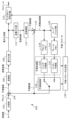
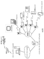
- FIG. 1 is a schematic diagram showing an example of the configuration of a transmission system according to an embodiment.
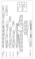
- FIG. 2 is a diagram showing an example of a hierarchical structure of data in a stream.
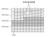
- FIG. 3 is a diagram showing an example of a slice configuration.
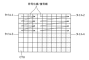
- FIG. 4 is a diagram showing an example of a tile configuration.
- FIG. 5 is a diagram showing an example of a coding structure during scalable coding.
- FIG. 6 is a diagram showing an example of a coding structure during scalable coding.
- FIG. 7 is a block diagram showing an example of the configuration of the encoding device according to the embodiment.
- FIG. 8 is a block diagram showing an implementation example of the encoding device.
- FIG. 1 is a schematic diagram showing an example of the configuration of a transmission system according to an embodiment.
- FIG. 2 is a diagram showing an example of a hierarchical structure of data in a stream.
- FIG. 3 is a diagram showing an example of a slice configuration.
- FIG. 9 is a flowchart illustrating an example of the overall encoding process by the encoding device.
- FIG. 10 is a diagram showing an example of block division.
- FIG. 11 is a diagram showing an example of the configuration of the dividing section.
- FIG. 12 is a diagram showing an example of a division pattern.
- FIG. 13A is a diagram illustrating an example of a syntax tree of a division pattern.
- FIG. 13B is a diagram showing another example of the syntax tree of the division pattern.
- FIG. 14 is a table showing transformation basis functions corresponding to each transformation type.
- FIG. 15 is a diagram showing an example of SVT.
- FIG. 16 is a flowchart illustrating an example of processing by the converter.
- FIG. 17 is a flowchart illustrating another example of processing by the converter.
- FIG. 16 is a flowchart illustrating an example of processing by the converter.
- FIG. 18 is a block diagram showing an example of the configuration of the quantization section.
- FIG. 19 is a flowchart showing an example of quantization by the quantization unit.
- FIG. 20 is a block diagram showing an example of the configuration of the entropy encoding section.
- FIG. 21 is a diagram showing the flow of CABAC in the entropy encoder.
- FIG. 22 is a block diagram showing an example of the configuration of the loop filter section.
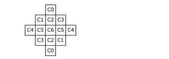
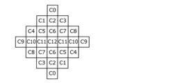
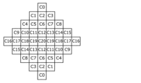
- FIG. 23A is a diagram illustrating an example of the shape of a filter used in an adaptive loop filter (ALF).
- FIG. 23B is a diagram showing another example of the shape of a filter used in ALF.
- FIG. 23C is a diagram showing another example of the shape of a filter used in ALF.
- FIG. ALF adaptive loop filter
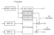
- FIG. 23D is a diagram showing an example in which the Y sample (first component) is used for Cb CCALF and Cr CCALF (multiple components different from the first component).
- FIG. 23E shows a diamond shaped filter.
- FIG. 23F is a diagram showing an example of JC-CCALF.
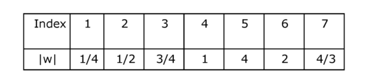
- FIG. 23G is a diagram illustrating an example of weight_index candidates for JC-CCALF.
- FIG. 24 is a block diagram showing an example of a detailed configuration of a loop filter section that functions as a DBF.
- FIG. 25 is a diagram illustrating an example of a deblocking filter having filter characteristics that are symmetrical with respect to block boundaries.
- FIG. 26 is a diagram for explaining an example of block boundaries on which deblocking filter processing is performed.
- FIG. 27 is a diagram showing an example of the Bs value.
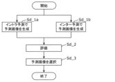
- FIG. 28 is a flowchart illustrating an example of processing performed by the prediction unit of the encoding device.
- FIG. 29 is a flowchart showing another example of processing performed by the prediction unit of the encoding device.
- FIG. 30 is a flowchart illustrating another example of processing performed by the prediction unit of the encoding device.
- FIG. 31 is a diagram showing an example of 67 intra prediction modes in intra prediction.
- FIG. 32 is a flowchart illustrating an example of processing by the intra prediction unit.
- FIG. 33 is a diagram showing an example of each reference picture.
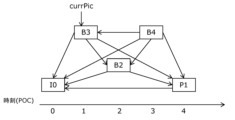
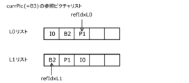
- FIG. 34 is a conceptual diagram showing an example of a reference picture list.
- FIG. 35 is a flowchart showing the basic processing flow of inter prediction.
- FIG. 28 is a flowchart illustrating an example of processing performed by the prediction unit of the encoding device.
- FIG. 29 is a flowchart showing another example of processing performed by the prediction unit
- FIG. 36 is a flowchart showing an example of MV derivation.
- FIG. 37 is a flowchart showing another example of MV derivation.
- FIG. 38A is a diagram illustrating an example of classification of each mode of MV derivation.
- FIG. 38B is a diagram illustrating an example of classification of each mode of MV derivation.
- FIG. 39 is a flowchart illustrating an example of inter prediction in normal inter mode.
- FIG. 40 is a flowchart illustrating an example of inter prediction in normal merge mode.
- FIG. 41 is a diagram for explaining an example of MV derivation processing in normal merge mode.
- FIG. 42 is a diagram for explaining an example of MV derivation processing in HMVP (History-based Motion Vector Prediction/Predictor) mode.
- FIG. HMVP History-based Motion Vector Prediction/Predictor
- FIG. 43 is a flowchart illustrating an example of FRUC (frame rate up conversion).
- FIG. 44 is a diagram for explaining an example of pattern matching (bilateral matching) between two blocks along a motion trajectory.
- FIG. 45 is a diagram for explaining an example of pattern matching (template matching) between a template in the current picture and a block in the reference picture.
- FIG. 46A is a diagram for explaining an example of deriving MV in sub-block units in affine mode using two control points.
- FIG. 46B is a diagram for explaining an example of deriving MV in sub-block units in affine mode using three control points.
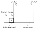
- FIG. 47A is a conceptual diagram for explaining an example of MV derivation of control points in affine mode.
- FIG. 47B is a conceptual diagram for explaining an example of MV derivation of control points in affine mode.
- FIG. 47C is a conceptual diagram for explaining an example of MV derivation of control points in affine mode.
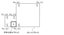
- FIG. 48A is a diagram for explaining an affine mode having two control points.
- FIG. 48B is a diagram for explaining an affine mode having three control points.
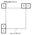
- FIG. 49A is a conceptual diagram for explaining an example of a control point MV derivation method when the number of control points is different between the encoded block and the current block.
- FIG. 49B is a conceptual diagram for explaining another example of the MV derivation method for control points when the number of control points is different between the encoded block and the current block.
- FIG. 49A is a conceptual diagram for explaining an example of a control point MV derivation method when the number of control points is different between the encoded block and the current block.
- FIG. 49B is a conceptual diagram for explaining another example of the MV de
- FIG. 50 is a flowchart illustrating an example of affine merge mode processing.
- FIG. 51 is a flowchart illustrating an example of processing in affine inter mode.
- FIG. 52A is a diagram for explaining generation of predicted images of two triangles.
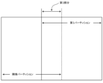
- FIG. 52B is a conceptual diagram showing an example of the first part of the first partition, the first sample set, and the second sample set.
- FIG. 52C is a conceptual diagram showing the first portion of the first partition.
- FIG. 53 is a flowchart showing an example of the triangle mode.
- FIG. 54 is a diagram illustrating an example of an ATMVP (Advanced Temporal Motion Vector Prediction/Predictor) mode in which MV is derived in sub-block units.
- FIG. ATMVP Advanced Temporal Motion Vector Prediction/Predictor
- FIG. 55 is a diagram showing the relationship between merge mode and DMVR (dynamic motion vector refreshing).
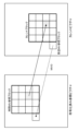
- FIG. 56 is a conceptual diagram for explaining an example of DMVR.
- FIG. 57 is a conceptual diagram for explaining another example of DMVR for determining MV.
- FIG. 58A is a diagram illustrating an example of motion search in DMVR.
- FIG. 58B is a flowchart illustrating an example of motion search in DMVR.
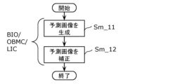
- FIG. 59 is a flowchart illustrating an example of generating a predicted image.
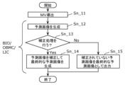
- FIG. 60 is a flowchart showing another example of generating a predicted image.
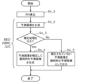
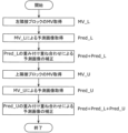
- FIG. 61 is a flowchart for explaining an example of predicted image correction processing by OBMC (overlapped block motion compensation).
- FIG. OBMC overlapped block motion compensation
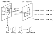
- FIG. 62 is a conceptual diagram for explaining an example of predicted image correction processing by OBMC.
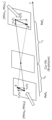
- FIG. 63 is a diagram for explaining a model assuming uniform linear motion.
- FIG. 64 is a flowchart illustrating an example of inter prediction according to BIO.
- FIG. 65 is a diagram illustrating an example of the configuration of an inter prediction unit that performs inter prediction according to BIO.
- FIG. 66A is a diagram for explaining an example of a predicted image generation method using brightness correction processing using LIC (local illumination compensation).
- FIG. 66B is a flowchart illustrating an example of a predicted image generation method using brightness correction processing by LIC.
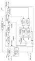
- FIG. 67 is a block diagram showing the configuration of a decoding device according to an embodiment.
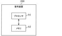
- FIG. 68 is a block diagram showing an implementation example of a decoding device.
- FIG. 69 is a flowchart illustrating an example of the overall decoding process by the decoding device.
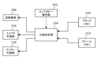
- FIG. 70 is a diagram showing the relationship between the division determining section and other components.
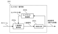
- FIG. 71 is a block diagram showing an example of the configuration of an entropy decoding section.
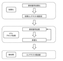
- FIG. 72 is a diagram showing the flow of CABAC in the entropy decoding section.
- FIG. 73 is a block diagram showing an example of the configuration of the inverse quantization section.
- FIG. 74 is a flowchart illustrating an example of inverse quantization by the inverse quantization unit.
- FIG. 75 is a flowchart illustrating an example of processing by the inverse transformer.
- FIG. 71 is a block diagram showing an example of the configuration of an entropy decoding section.
- FIG. 72 is a diagram showing the flow of CABAC in the entropy decoding section.
- FIG. 76 is a flowchart showing another example of processing by the inverse transformer.
- FIG. 77 is a block diagram showing an example of the configuration of the loop filter section.
- FIG. 78 is a flowchart illustrating an example of processing performed by the prediction unit of the decoding device.
- FIG. 79 is a flowchart showing another example of processing performed by the prediction unit of the decoding device.
- FIG. 80A is a flowchart showing part of another example of processing performed by the prediction unit of the decoding device.
- FIG. 80B is a flowchart showing the remainder of another example of processing performed by the prediction unit of the decoding device.
- FIG. 81 is a diagram illustrating an example of processing by the intra prediction unit of the decoding device.
- FIG. 82 is a flowchart showing an example of MV derivation in the decoding device.
- FIG. 83 is a flowchart showing another example of MV derivation in the decoding device.
- FIG. 84 is a flowchart illustrating an example of inter prediction in normal inter mode in the decoding device.
- FIG. 85 is a flowchart illustrating an example of inter prediction in normal merge mode in the decoding device.
- FIG. 86 is a flowchart illustrating an example of inter prediction in FRUC mode in the decoding device.
- FIG. 87 is a flowchart illustrating an example of inter prediction using affine merge mode in the decoding device.
- FIG. 88 is a flowchart illustrating an example of inter prediction using affine inter mode in the decoding device.
- FIG. 89 is a flowchart illustrating an example of inter prediction in triangle mode in the decoding device.
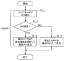
- FIG. 90 is a flowchart illustrating an example of motion search using DMVR in the decoding device.
- FIG. 91 is a flowchart showing a detailed example of motion search using DMVR in the decoding device.
- FIG. 92 is a flowchart illustrating an example of generation of a predicted image in the decoding device.
- FIG. 93 is a flowchart showing another example of generating a predicted image in the decoding device.
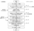
- FIG. 94 is a flowchart illustrating an example of correction of a predicted image by OBMC in a decoding device.
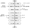
- FIG. 95 is a flowchart illustrating an example of correction of a predicted image by BIO in a decoding device.
- FIG. 96 is a flowchart illustrating an example of correction of a predicted image by LIC in the decoding device.
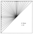
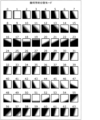
- FIG. 97 is a conceptual diagram showing a plurality of geometric division modes according to VVC.
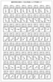
- FIG. 98 is a conceptual diagram showing an example of the mapping relationship between a plurality of geometric division modes and a plurality of angular intra prediction modes.
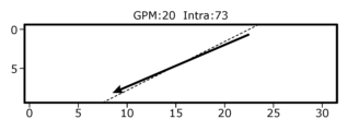
- FIG. 99 is a conceptual diagram showing an example of the mapping relationship between one geometric division mode and one angular intra prediction mode.
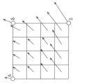
- FIG. 100 is a conceptual diagram illustrating an example of multiple intra prediction modes including multiple narrow-angle intra prediction modes and multiple wide-angle intra prediction modes.
- FIG. 101A is a conceptual diagram showing a first example of the relationship between the geometric division mode and the wide-angle intra prediction mode.
- FIG. 101B is a conceptual diagram showing a second example of the relationship between the geometric division mode and the wide-angle intra prediction mode.
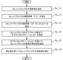
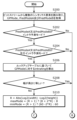
- FIG. 102A is a flowchart illustrating part of the operation for determining parameters of the geometric division mode.
- FIG. 102B is a flowchart illustrating the remainder of the operations for determining the parameters of the geometric splitting mode.
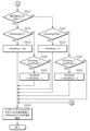
- FIG. 103A is a flowchart illustrating part of the operation of making predictions according to the geometric partitioning mode.
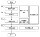
- FIG. 103B is a flowchart illustrating the remainder of the operations for making predictions according to the geometric partitioning mode.
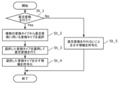
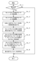
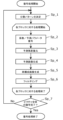
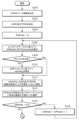
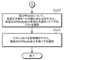
- FIG. 104 is a flowchart showing operations performed by the encoding device according to the embodiment.
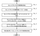
- FIG. 105 is a flowchart showing operations performed by the decoding device according to the embodiment.
- FIG. 106 is an overall configuration diagram of a content supply system that realizes a content distribution service.
- FIG. 107 is a diagram showing an example of a display screen of a web page.
- FIG. 108 is a diagram showing an example of a display screen of a web page.
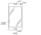
- FIG. 109 is a diagram illustrating an example of a smartphone.
- FIG. 110 is a block diagram showing an example of the configuration of a smartphone.
- Geometric division mode is also called GPM or GPM mode.
- GPM geometric division mode
- a prediction for the block is then generated by a combination of the prediction for one partition and the prediction for the other partition. This may improve prediction accuracy.
- intra prediction may be used for at least one of the two partitions.
- an intra prediction mode corresponding to the direction of the dividing line in the geometric dividing mode may be specified.
- a narrow-angle intra prediction mode that satisfies a certain condition may be mapped to a wide-angle intra prediction mode, and the wide-angle intra prediction mode may be used for prediction.
- a narrow-angle intra prediction mode that satisfies certain conditions becomes a wide-angle intra prediction mode that is shifted from a wide-angle intra prediction mode that has a prediction direction opposite to that of the narrow-angle intra prediction mode. May be mapped. Therefore, for non-square blocks, the narrow-angle intra prediction mode that corresponds to the direction of the dividing line in the geometric partitioning mode is mapped to the wide-angle intra prediction mode that does not correspond to the direction of the dividing line in the geometric partitioning mode. there is a possibility.
- an accurate prediction direction may not be used for non-square blocks, and prediction accuracy may deteriorate.
- the decoding method of Example 1 is a decoding method for decoding a current block of a video from a bitstream, in which two partitions in the current block are determined according to a geometric division mode, and a plurality of geometric division modes are used. and a plurality of angular intra prediction modes to derive an angular intra prediction mode from the geometric partitioning mode, and predict a first partition of the two partitions according to the angular intra prediction mode.
- the angular intra prediction mode when the shape of the current block is a square, the first mapping relationship is used as the mapping relationship to derive the angular intra prediction mode, and the shape of the current block is not a square.
- the angular intra prediction mode is derived using a second mapping relationship different from the first mapping relationship as the mapping relationship.
- the decoding method of Example 2 is the decoding method of Example 1, wherein the first mapping relationship includes a mapping relationship between the geometric division mode and the first narrow-angle intra prediction mode, and the second mapping relationship includes a mapping relationship between the geometric division mode and the first narrow-angle intra prediction mode.
- the relationship includes a mapping relationship between the geometric division mode and a second narrow-angle intra prediction mode, and when the first narrow-angle intra prediction mode is included in a subset of the plurality of angular intra prediction modes, (i )
- the second narrow-angle intra prediction mode is a prediction direction of the first narrow-angle intra prediction mode.
- the second narrow-angle intra prediction mode has a second index value obtained by applying a fixed offset value addition or subtraction to the first index value of the first narrow-angle intra prediction mode, is remapped to the wide-angle intra prediction mode, and is remapped to the wide-angle intra prediction mode;
- the second narrow-angle intra prediction mode is the same as the first narrow-angle intra prediction mode, Good too.
- the decoding method of Example 3 may be the decoding method of Example 2, in which the fixed offset value is 1.
- the decoding method of Example 4 is the decoding method of Example 2 or Example 3, in which the subset of the plurality of angular intra prediction modes is determined by the difference between the width and height of the current block. It's okay.
- This may make it possible to define a narrow-angle intra prediction mode in which a mapping different from that for a square block is applied according to the difference in width and height of the current block. Therefore, it may be possible to adjust the prediction direction according to the difference in width and height of the current block. Therefore, it may be possible to perform intra prediction using an accurate prediction direction.
- the decoding method of Example 5 is the decoding method of any of Examples 2 to 4, wherein the prediction direction of the first narrow-angle intra prediction mode is parallel to the boundary between the two partitions,
- the decoding method may be such that the prediction direction of the wide-angle intra prediction mode is parallel to the boundary.
- This may make it possible to perform intra prediction using a prediction direction that corresponds to the boundary between two partitions determined in the geometric partitioning mode. Therefore, deterioration in prediction accuracy may be suppressed.
- the decoding method of Example 6 is the decoding method of any one of Examples 2 to 4, wherein the prediction direction of the first narrow-angle intra prediction mode is at a constant angle with respect to the boundary between the two partitions.
- the decoding method may be such that the prediction direction of the wide-angle intra prediction mode has the constant angle with respect to the boundary.
- This may make it possible to perform intra prediction using the prediction direction related to the boundary between the two partitions determined in the geometric partitioning mode. Therefore, deterioration in prediction accuracy may be suppressed.
- the decoding method of Example 7 is the decoding method of Example 1, wherein the first mapping relationship is between the plurality of geometric division modes and the plurality of angular intra predictions which are the plurality of narrow angle intra prediction modes. mode, and the second mapping relationship is a mapping relationship between the plurality of geometric division modes and the plurality of angular intra prediction modes including a plurality of narrow-angle intra prediction modes and one or more wide-angle intra prediction modes.
- the decoding method may be a mapping relationship between
- This may allow mapping the geometric partitioning mode to the wide-angle intra prediction mode for non-square blocks. Therefore, it may be possible to perform intra prediction using an accurate prediction direction.
- the decoding method of Example 8 is the decoding method of any one of Examples 1 to 7, and includes a first prediction mode indicator indicating a prediction method of the first partition, and a second prediction mode indicator of the second partition of the two partitions. a second prediction mode indicator indicating how to predict a partition is decoded from the bitstream, and the first prediction mode indicator is such that the angular intra prediction mode derived from the geometric partitioning mode
- the decoding method may be used as a prediction method for the first partition.
- This may make it possible to control the prediction methods of each of the two partitions. Then, it may be possible to control application of the intra prediction mode corresponding to the geometric partitioning mode to the first partition.
- the encoding method of Example 9 is an encoding method for encoding a current block of a video into a bit stream, in which two partitions in the current block are determined according to a geometric partition mode, and a plurality of geometric partitions are determined. derive an angular intra prediction mode from the geometric partition mode using a mapping relationship between a geometric partition mode and a plurality of angular intra prediction modes; and according to the angular intra prediction mode, a first partition of the two partitions is In the derivation of the angular intra prediction mode, when the shape of the current block is a square, the angular intra prediction mode is derived using the first mapping relation as the mapping relation, and the shape of the current block is calculated using the first mapping relation as the mapping relation. is not a square, the encoding method uses a second mapping relationship different from the first mapping relationship as the mapping relationship to derive the angular intra prediction mode.
- the encoding method of Example 10 is the encoding method of Example 9, wherein the first mapping relationship includes a mapping relationship between the geometric division mode and the first narrow-angle intra prediction mode, and the first mapping relationship includes the mapping relationship between the geometric division mode and the first narrow-angle intra prediction mode.
- 2 mapping relationship includes a mapping relationship between the geometric division mode and a second narrow-angle intra prediction mode, and when the first narrow-angle intra prediction mode is included in a subset of the plurality of angular intra prediction modes, (i) When the prediction direction of the first narrow-angle intra prediction mode is at an angle of 45 degrees with respect to the horizontal or vertical direction, the second narrow-angle intra prediction mode is set to the first narrow-angle intra prediction mode.
- the second narrow-angle intra prediction mode has a prediction direction opposite to the prediction direction of The prediction mode has a second index value obtained by applying a fixed offset value addition or subtraction to the first index value of the first narrow-angle intra prediction mode, and is remapped to the wide-angle intra prediction mode, and In the case where the first narrow-angle intra prediction mode is not included in the subset of the plurality of angular intra-prediction modes, the second narrow-angle intra prediction mode is the same as the first narrow-angle intra prediction mode. It may be.
- the encoding method of Example 11 may be the encoding method of Example 10, in which the fixed offset value is 1.
- the encoding method of Example 12 is the encoding method of Example 10 or Example 11, wherein the subset of the plurality of angular intra prediction modes is determined by the difference between the width and height of the current block. It may be a method.
- This may make it possible to define a narrow-angle intra prediction mode in which a mapping different from that for a square block is applied according to the difference in width and height of the current block. Therefore, it may be possible to adjust the prediction direction according to the difference in width and height of the current block. Therefore, it may be possible to perform intra prediction using an accurate prediction direction.
- the encoding method of Example 13 is the encoding method of any one of Examples 10 to 12, and the prediction direction of the first narrow-angle intra prediction mode is parallel to the boundary between the two partitions.
- the encoding method may be such that the prediction direction of the wide-angle intra prediction mode is parallel to the boundary.
- This may make it possible to perform intra prediction using a prediction direction that corresponds to the boundary between two partitions determined in the geometric partitioning mode. Therefore, deterioration in prediction accuracy may be suppressed.
- the encoding method of Example 14 is the encoding method of any of Examples 10 to 12, and the prediction direction of the first narrow-angle intra prediction mode is relative to the boundary between the two partitions.
- the encoding method may have a certain angle, and the prediction direction of the wide-angle intra prediction mode may have the certain angle with respect to the boundary.
- This may make it possible to perform intra prediction using the prediction direction related to the boundary between the two partitions determined in the geometric partitioning mode. Therefore, deterioration in prediction accuracy may be suppressed.
- the encoding method of Example 15 is the encoding method of Example 9, wherein the first mapping relationship is between the plurality of geometric division modes and the plurality of angles which are the plurality of narrow-angle intra prediction modes.
- the second mapping relationship is a mapping relationship between the plurality of geometric division modes and the plurality of angular intra prediction modes including a plurality of narrow-angle intra prediction modes and one or more wide-angle intra prediction modes. It may be an encoding method that has a mapping relationship with a prediction mode.
- This may allow mapping the geometric partitioning mode to the wide-angle intra prediction mode for non-square blocks. Therefore, it may be possible to perform intra prediction using an accurate prediction direction.
- the encoding method of Example 16 is the encoding method of any one of Examples 9 to 15, and includes a first prediction mode indicator indicating a prediction method of the first partition, and a first prediction mode indicator indicating a prediction method of the first partition.
- a second prediction mode indicator is encoded in the bitstream indicating a prediction method for a second partition, and the first prediction mode indicator indicates that the angular intra prediction mode derived from the geometric partitioning mode is a prediction method for the first partition.
- the encoding method may indicate that it is used for prediction as a prediction method for the first partition.
- This may make it possible to control the prediction methods of each of the two partitions. Then, it may be possible to control application of the intra prediction mode corresponding to the geometric partitioning mode to the first partition.
- the non-transitory computer-readable recording medium of Example 17 is a non-transitory computer-readable recording medium for use in a computer, and stores a bitstream that causes a computer to perform a decoding process to decode a current block; In the decoding process, two partitions in the current block are determined according to the geometric partitioning mode, and the geometric partitioning is performed using mapping relationships between the plurality of geometric partitioning modes and the plurality of angular intra prediction modes.
- the method may be a non-transitory computer-readable recording medium for deriving the angular intra prediction mode.
- the decoding device of Example 18 is a decoding device for decoding a current block of video from a bitstream, comprising a circuit and a memory connected to the circuit, wherein the circuit operates according to a geometric partitioning mode. , determine two partitions in the current block, derive an angular intra prediction mode from the geometric partition mode using a mapping relationship between a plurality of geometric partition modes and a plurality of angular intra prediction modes, and predicting a first partition of the two partitions according to an angular intra prediction mode, and in deriving the angular intra prediction mode, if the shape of the current block is a square, a first mapping relationship is used as the mapping relationship; and deriving the angular intra prediction mode, and when the shape of the current block is not a square, using a second mapping relationship different from the first mapping relationship as the mapping relationship, deriving the angular intra prediction mode. It is a decoding device.
- the encoding device of Example 19 is an encoding device for encoding a current block of a video into a bitstream, and includes a circuit and a memory connected to the circuit, and the circuit operates in a geometric manner. determining two partitions in the current block according to the partitioning mode, and deriving an angular intra-prediction mode from the geometric partitioning mode using a mapping relationship between the plurality of geometric partitioning modes and the plurality of angular intra-prediction modes.
- the first mapping relationship is set to the mapping If the shape of the current block is not a square, a second mapping relationship different from the first mapping relationship is used as the mapping relationship to derive the angular intra prediction mode.
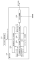
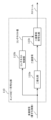
- the decoding device of Example 20 includes an input section, an entropy decoding section, an inverse quantization section, an inverse transformation section, an intra prediction section, an inter prediction section, a loop filter section, and an output section.
- An encoded bitstream is input to the input unit.
- the entropy decoding unit applies variable length decoding to the encoded bitstream to derive quantization coefficients.
- the dequantization unit dequantizes the quantized coefficients and derives transform coefficients.
- the inverse transformer inversely transforms the transform coefficients to derive a prediction error.
- the intra prediction unit generates a prediction signal of a current block included in the current picture using reference pixels included in the current picture.
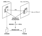
- the inter prediction unit generates a prediction signal of a current block included in the current picture using a reference block included in a reference picture different from the current picture.
- the loop filter section applies a filter to the reconstructed block of the current block included in the current picture. Then, the current picture is output from the output unit.
- the intra prediction unit determines two partitions in the current block according to the geometric partition mode, and uses the mapping relationship between the plurality of geometric partition modes and the plurality of angular intra prediction modes. , derive an angular intra prediction mode from the geometric partitioning mode, predict a first partition of the two partitions according to the angular intra prediction mode, and in deriving the angular intra prediction mode, If the shape is a square, a first mapping relationship is used as the mapping relationship to derive the angular intra prediction mode, and if the shape of the current block is not a square, a second mapping relationship different from the first mapping relationship. is used as the mapping relationship to derive the angular intra prediction mode.
- the encoding device of Example 21 includes an input section, a division section, an intra prediction section, an inter prediction section, a loop filter section, a transformation section, a quantization section, an entropy encoding section, and an output section. Equipped with.
- a current picture is input to the input section.
- the dividing unit divides the current picture into a plurality of blocks.
- the intra prediction unit generates a prediction signal of a current block included in the current picture using reference pixels included in the current picture.
- the inter prediction unit generates a prediction signal of a current block included in the current picture using a reference block included in a reference picture different from the current picture.
- the loop filter section applies a filter to a reconstructed block of the current block included in the current picture.
- the conversion unit converts a prediction error between an original signal of the current block included in the current picture and a prediction signal generated by the intra prediction unit or the inter prediction unit to generate conversion coefficients.
- the quantization unit quantizes the transform coefficients to generate quantized coefficients.
- the entropy encoding unit applies variable length encoding to the quantized coefficients to generate an encoded bitstream. Then, the encoded bitstream including the quantized coefficients subjected to variable length encoding and control information is output from the output unit.
- the intra prediction unit determines two partitions in the current block according to the geometric partition mode, and uses the mapping relationship between the plurality of geometric partition modes and the plurality of angular intra prediction modes. , derive an angular intra prediction mode from the geometric partitioning mode, predict a first partition of the two partitions according to the angular intra prediction mode, and in deriving the angular intra prediction mode, If the shape is a square, a first mapping relationship is used as the mapping relationship to derive the angular intra prediction mode, and if the shape of the current block is not a square, a second mapping relationship different from the first mapping relationship. is used as the mapping relationship to derive the angular intra prediction mode.
- Image A unit of data composed of a set of pixels, consisting of a picture or a block smaller than a picture, and includes still images as well as moving images.
- Picture A unit of image processing made up of a set of pixels, and is sometimes called a frame or field.
- Block This is a processing unit of a set including a specific number of pixels, and as shown in the example below, the name does not matter.
- the shape is not limited, and includes, for example, a rectangle made up of M ⁇ N pixels, a square made up of M ⁇ M pixels, as well as a triangle, a circle, and other shapes.
- Pixel value/sample value A unique value that a pixel has, and includes not only a luminance value, a color difference value, and RGB gradations, but also a depth value or binary values of 0 and 1.
- the flag may be a plurality of bits, for example, it may be a parameter or index of 2 or more bits. Moreover, not only binary numbers using binary numbers but also multi-values using other base numbers may be used.
- Signal A signal is something that is encoded or encoded to convey information, and includes not only discrete digital signals but also analog signals that take continuous values.
- Stream/Bitstream A data string of digital data or a flow of digital data.
- the stream/bitstream may be composed of a single stream or a plurality of streams divided into a plurality of layers.
- data is transmitted by serial communication over a single transmission path, it also includes the case where it is transmitted by packet communication through a plurality of transmission paths.
- Color difference (chroma) Adjectives denoted by the symbols Cb and Cr, specifying that a sample array or a single sample represents one of two color difference signals related to primary colors. Instead of the term chroma, the term chrominance can also be used.
- Luminance An adjective represented by a symbol or subscript Y or L specifying that a sample array or a single sample represents a monochrome signal related to a primary color. Instead of the term luma, the term luminance can also be used.
- an encoding device and a decoding device will be described.
- the embodiments are examples of an encoding device and a decoding device to which the processing and/or configuration described in each aspect of the present disclosure can be applied.
- the processing and/or configuration can also be implemented in an encoding device and a decoding device different from those in the embodiment.
- any of the following may be implemented.
- Some of the components of the plurality of components constituting the encoding device or decoding device of the embodiment may be combined with the components described in any of the aspects of the present disclosure. , may be combined with a component having part of the functions described in any of the aspects of the present disclosure, or a component that performs part of the processing performed by the component described in each aspect of the present disclosure. May be combined with
- Components that have part of the functions of the encoding device or decoding device according to the embodiment, or components that implement a part of the processing of the encoding device or decoding device according to the embodiment are those according to the present disclosure.
- any of the plurality of processes included in the method is the same as the process described in any of the aspects of the present disclosure, or similar to the process described in any of the aspects of the present disclosure. It may be replaced or combined with any of the treatments.
- the method of implementing the processing and/or configuration described in each aspect of the present disclosure is not limited to the encoding device or decoding device of the embodiment.
- the processing and/or configuration may be performed in an apparatus used for a purpose different from video encoding or video decoding disclosed in the embodiments.
- FIG. 1 is a schematic diagram showing an example of the configuration of a transmission system according to this embodiment.
- the transmission system Trs is a system that transmits a stream generated by encoding an image and decodes the transmitted stream.
- Such a transmission system Trs includes an encoding device 100, a network Nw, and a decoding device 200, as shown in FIG. 1, for example.
- An image is input to the encoding device 100.
- the encoding device 100 generates a stream by encoding the input image, and outputs the stream to the network Nw.
- the stream includes, for example, an encoded image and control information for decoding the encoded image.
- the image is compressed by this encoding.
- the original image before being encoded that is input to the encoding device 100 is also referred to as an original image, an original signal, or an original sample.
- the image may be a moving image or a still image.
- an image is a generic concept such as a sequence, a picture, and a block, and unless otherwise specified, it is not limited by spatial and temporal regions.
- an image consists of an array of pixels or pixel values, and the signals or pixel values representing the image are also called samples.
- a stream may also be called a bitstream, encoded bitstream, compressed bitstream, or encoded signal.
- the encoding device may be called an image encoding device or a video encoding device, and the encoding method by the encoding device 100 is an encoding method, an image encoding method, or a video encoding method. may be called.
- the network Nw transmits the stream generated by the encoding device 100 to the decoding device 200.
- the network Nw may be the Internet, a wide area network (WAN), a local area network (LAN), or a combination thereof.
- the network Nw is not necessarily a two-way communication network, but may be a one-way communication network that transmits broadcast waves such as terrestrial digital broadcasting or satellite broadcasting. Further, the network Nw may be replaced by a storage medium on which a stream is recorded, such as a DVD (Digital Versatile Disc) or a BD (Blu-Ray Disc (registered trademark)).
- the decoding device 200 generates a decoded image, which is an uncompressed image, for example, by decoding the stream transmitted by the network Nw. For example, the decoding device decodes the stream according to a decoding method that corresponds to the encoding method used by the encoding device 100.
- the decoding device may be called an image decoding device or a moving image decoding device, and the decoding method by the decoding device 200 may be called a decoding method, an image decoding method, or a moving image decoding method.
- FIG. 2 is a diagram showing an example of a hierarchical structure of data in a stream.
- a stream includes, for example, a video sequence.
- this video sequence includes a VPS (Video Parameter Set), an SPS (Sequence Parameter Set), a PPS (Picture Parameter Set), and an SEI (Supplemental Enhancement Set). ancement Information) and multiple Contains pictures of.
- VPS Video Parameter Set
- SPS Sequence Parameter Set
- PPS Position Parameter Set
- SEI Supplemental Enhancement Set
- ancement Information Supplemental Enhancement Set
- VPS includes encoding parameters common to the multiple layers and encoding parameters related to the multiple layers included in the video or individual layers.
- the SPS includes parameters used for the sequence, that is, encoding parameters that the decoding device 200 refers to in order to decode the sequence.
- the encoding parameter may indicate the width or height of the picture. Note that a plurality of SPSs may exist.
- the PPS includes parameters used for the picture, that is, encoding parameters that the decoding device 200 refers to in order to decode each picture in the sequence.
- the encoding parameters may include a reference value for the quantization width used in decoding the picture and a flag indicating application of weighted prediction. Note that a plurality of PPSs may exist. Further, SPS and PPS are sometimes simply called parameter sets.
- a picture may include a picture header and one or more slices, as shown in FIG. 2(b).
- the picture header includes encoding parameters referenced by decoding device 200 to decode its one or more slices.
- a slice includes a slice header and one or more bricks, as shown in FIG. 2(c).
- the slice header includes encoding parameters referenced by decoding device 200 to decode the one or more bricks.
- the brick includes one or more CTUs (Coding Tree Units).
- CTUs Coding Tree Units
- a picture may not include a slice and instead of the slice, it may include a tile group.
- the tile group includes one or more tiles.
- the brick may include slices.
- a CTU is also called a superblock or basic division unit.
- Such a CTU includes a CTU header and one or more CUs (Coding Units), as shown in FIG. 2(e).
- the CTU header includes encoding parameters that the decoding device 200 refers to in order to decode one or more CUs.
- a CU may be divided into multiple smaller CUs. Further, as shown in FIG. 2(f), the CU includes a CU header, prediction information, and residual coefficient information.
- the prediction information is information for predicting the CU
- the residual coefficient information is information indicating a prediction residual, which will be described later.
- a CU is basically the same as a PU (Prediction Unit) and a TU (Transform Unit), but for example, in an SBT described below, it may include a plurality of TUs smaller than the CU.
- a CU may be processed for each VPDU (Virtual Pipeline Decoding Unit) that constitutes the CU.
- a VPDU is a fixed unit that can be processed in one stage when performing pipeline processing in hardware, for example.
- a picture that is currently being processed by a device such as the encoding device 100 or the decoding device 200 is referred to as a current picture. If the process is encoding, the current picture is synonymous with the picture to be encoded, and if the process is decoding, the current picture is synonymous with the picture to be decoded. Further, a block such as a CU or a CU that is currently being processed by a device such as the encoding device 100 or the decoding device 200 is referred to as a current block. If the process is encoding, the current block has the same meaning as the block to be encoded, and if the process is decoding, the current block has the same meaning as the block to be decoded.
- pictures may be configured in units of slices or tiles.
- a slice is a basic encoding unit that makes up a picture.
- a picture is composed of, for example, one or more slices.
- a slice consists of one or more consecutive CTUs.
- FIG. 3 is a diagram showing an example of a slice configuration.
- a picture includes 11 ⁇ 8 CTUs and is divided into four slices (slices 1-4).
- Slice 1 consists of, for example, 16 CTUs
- slice 2 consists of, for example, 21 CTUs
- slice 3 consists of, for example, 29 CTUs
- slice 4 consists of, for example, 22 CTUs.
- each CTU within a picture belongs to one of the slices.
- the shape of a slice is a picture divided horizontally.
- the slice boundary does not need to be at the screen edge, but may be anywhere among the CTU boundaries within the screen.
- the processing order (encoding order or decoding order) of CTUs in a slice is, for example, raster scan order.
- a slice includes a slice header and encoded data.
- the slice header may describe characteristics of the slice, such as the CTU address at the beginning of the slice and the slice type.
- a tile is a unit of rectangular area that makes up a picture.
- Each tile may be assigned a number called TileId in raster scan order.
- FIG. 4 is a diagram showing an example of a tile configuration.
- a picture includes 11 ⁇ 8 CTUs and is divided into four rectangular area tiles (tiles 1-4).
- the processing order of CTUs is changed compared to when tiles are not used. If tiles are not used, CTUs within a picture are processed, for example, in raster scan order. If tiles are used, at least one CTU is processed in each of the plurality of tiles, eg, in raster scan order.
- the processing order of multiple CTUs included in tile 1 is from the left end of the first column of tile 1 to the right end of the first column of tile 1, and then to the left end of the second column of tile 1. The order is from tile 1 to the right end of the second row.
- one tile may include one or more slices, and one slice may include one or more tiles.
- a tile set may include one or more tile groups and may include one or more tiles.
- a picture may be composed of only one of a tile set, a tile group, and a tile.
- the basic coding order of tiles is the order in which a plurality of tiles are scanned in raster order for each tile set.
- a tile group is a collection of one or more tiles with consecutive basic encoding orders within each tile set.
- Such a picture may be constructed by the dividing unit 102 (see FIG. 7), which will be described later.
- [Scalable encoding] 5 and 6 are diagrams illustrating an example of a scalable stream configuration.
- the encoding device 100 may generate a temporally/spatially scalable stream by dividing and encoding each of a plurality of pictures into one of a plurality of layers.
- the encoding device 100 achieves scalability in which an enhancement layer exists above a base layer by encoding a picture for each layer.
- This kind of encoding of each picture is called scalable encoding.
- the decoding device 200 can switch the image quality of the displayed image by decoding the stream. That is, the decoding device 200 determines which layer to decode according to internal factors such as its own performance and external factors such as the state of the communication band.
- the decoding device 200 can freely switch and decode the same content into low-resolution content and high-resolution content.
- a user of the stream may use a smartphone to view part of the video stream while on the move, and then view the rest of the video video using a device such as an Internet TV after returning home.
- a device such as an Internet TV after returning home.
- each of the above-mentioned smartphones and devices incorporates a decoding device 200 having the same or different performance. In this case, if the device decodes up to the upper layer of the stream, the user can watch high-quality moving images after returning home. Thereby, the encoding device 100 does not need to generate multiple streams with the same content but different image quality, and can reduce the processing load.
- the enhancement layer may include meta information based on image statistical information or the like.
- the decoding device 200 may generate a high-quality moving image by super-resolving the base layer picture based on the meta information.
- Super-resolution may be either an improvement in the signal-to-noise (SN) ratio at the same resolution or an expansion of the resolution.
- Meta information includes information for specifying linear or nonlinear filter coefficients used in super-resolution processing, information for specifying parameter values in filter processing, machine learning, or least squares calculations used for super-resolution processing, etc. It's okay to stay.
- the picture may be divided into tiles etc. depending on the meaning of each object in the picture.
- the decoding device 200 may decode only a partial area of the picture by selecting a tile to be decoded.
- attributes of objects person, car, ball, etc.
- positions within a picture may be stored as meta information.
- the decoding device 200 can specify the position of the desired object based on the meta information and determine the tile that includes the object. For example, as shown in FIG. 6, meta information is stored using a different data storage structure than image data, such as SEI in HEVC. This meta information indicates, for example, the position, size, or color of the main object.
- meta information may be stored in units consisting of multiple pictures, such as streams, sequences, or random access units.
- the decoding device 200 can obtain the time at which a specific person appears in a video image, and by using that time and information on a per-picture basis, the decoding device 200 can identify the picture in which the object exists and the object within that picture. The location can be determined.
- FIG. 7 is a block diagram illustrating an example of the configuration of encoding device 100 according to the embodiment.
- the encoding device 100 encodes an image in units of blocks.
- the encoding device 100 is a device that encodes an image in block units, and includes a dividing unit 102, a subtracting unit 104, a converting unit 106, a quantizing unit 108, and an entropy encoding unit.
- section 110 inverse quantization section 112, inverse transformation section 114, addition section 116, block memory 118, loop filter section 120, frame memory 122, intra prediction section 124, inter prediction section 126, It includes a prediction control section 128 and a prediction parameter generation section 130.
- each of the intra prediction unit 124 and the inter prediction unit 126 is configured as a part of a prediction processing unit.
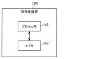
- FIG. 8 is a block diagram showing an implementation example of the encoding device 100.
- Encoding device 100 includes a processor a1 and a memory a2.
- multiple components of the encoding device 100 shown in FIG. 7 are implemented by the processor a1 and memory a2 shown in FIG. 8.
- the processor a1 is a circuit that performs information processing and is a circuit that can access the memory a2.
- processor a1 is a dedicated or general-purpose electronic circuit that encodes images.
- Processor a1 may be a processor such as a CPU.
- the processor a1 may be a collection of a plurality of electronic circuits.
- the processor a1 may play the role of a plurality of components other than a component for storing information among the plurality of components of the encoding device 100 shown in FIG. 7.
- the memory a2 is a dedicated or general-purpose memory in which information for the processor a1 to encode an image is stored.
- Memory a2 may be an electronic circuit and may be connected to processor a1. Furthermore, the memory a2 may be included in the processor a1. Furthermore, the memory a2 may be a collection of a plurality of electronic circuits. Furthermore, the memory a2 may be a magnetic disk, an optical disk, or the like, or may be expressed as a storage, a recording medium, or the like. Further, the memory a2 may be a nonvolatile memory or a volatile memory.
- the memory a2 may store an image to be encoded, or may store a stream corresponding to the encoded image. Furthermore, a program for the processor a1 to encode an image may be stored in the memory a2.
- the memory a2 may serve as a component for storing information among the multiple components of the encoding device 100 shown in FIG. 7.
- memory a2 may serve as block memory 118 and frame memory 122 shown in FIG.
- a reconstructed image (specifically, a reconstructed block, a reconstructed picture, etc.) may be stored in the memory a2.
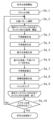
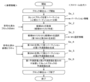
- FIG. 9 is a flowchart illustrating an example of the overall encoding process by the encoding device 100.
- the dividing unit 102 of the encoding device 100 divides the picture included in the original image into a plurality of fixed-sized blocks (128 ⁇ 128 pixels) (step Sa_1). Then, the dividing unit 102 selects a dividing pattern for the fixed size block (step Sa_2). That is, the dividing unit 102 further divides the fixed size block into a plurality of blocks forming the selected division pattern. Then, the encoding device 100 performs steps Sa_3 to Sa_9 on each of the plurality of blocks.
- the prediction processing unit consisting of the intra prediction unit 124 and the inter prediction unit 126 and the prediction control unit 128 generate a predicted image of the current block (step Sa_3).
- the predicted image is also called a predicted signal, a predicted block, or a predicted sample.
- the subtraction unit 104 generates the difference between the current block and the predicted image as a prediction residual (step Sa_4).
- the prediction residual is also called a prediction error.
- the transformation unit 106 and the quantization unit 108 generate a plurality of quantization coefficients by transforming and quantizing the predicted image (step Sa_5).
- the entropy encoding unit 110 generates a stream by encoding (specifically entropy encoding) the plurality of quantization coefficients and prediction parameters related to generation of the predicted image ( Step Sa_6).
- the inverse quantization unit 112 and the inverse transformation unit 114 restore the prediction residual by performing inverse quantization and inverse transformation on the plurality of quantized coefficients (step Sa_7).
- the adding unit 116 reconstructs the current block by adding the predicted image to the restored prediction residual (step Sa_8). As a result, a reconstructed image is generated.
- a reconstructed image is also called a reconstructed block, and in particular, a reconstructed image generated by the encoding device 100 is also called a local decoded block or a locally decoded image.
- the loop filter unit 120 performs filtering on the reconstructed image as necessary (step Sa_9).
- step Sa_10 determines whether encoding of the entire picture has been completed (step Sa_10), and when determining that encoding has not been completed (No in step Sa_10), repeats the process from step Sa_2. do.
- the encoding device 100 selects one division pattern for a fixed-size block and encodes each block according to the division pattern, but encodes each block according to each of the plurality of division patterns. Each block may also be encoded. In this case, the encoding device 100 evaluates the cost of each of the plurality of division patterns, and selects, for example, the stream obtained by encoding according to the division pattern with the lowest cost as the stream to be finally output. You may.
- processing of these steps Sa_1 to Sa_10 may be performed sequentially by the encoding device 100, or some of the processing may be performed in parallel, and the order may be changed. It's okay.
- the encoding process performed by such encoding device 100 is hybrid encoding using predictive encoding and transform encoding.
- Predictive coding also includes a subtraction unit 104, a conversion unit 106, a quantization unit 108, an inverse quantization unit 112, an inverse transformation unit 114, an addition unit 116, a loop filter unit 120, a block memory 118, a frame memory 122, and intra prediction.
- This is performed by an encoding loop consisting of a prediction unit 124, an inter prediction unit 126, and a prediction control unit 128.
- the prediction processing unit including the intra prediction unit 124 and the inter prediction unit 126 constitutes a part of the encoding loop.
- the dividing unit 102 divides each picture included in the original image into a plurality of blocks, and outputs each block to the subtracting unit 104.
- the dividing unit 102 first divides the picture into blocks of a fixed size (for example, 128x128 pixels).
- This fixed size block is sometimes called a coding tree unit (CTU).
- the dividing unit 102 then divides each of the fixed size blocks into blocks of variable size (for example, 64x64 pixels or less) based on, for example, recursive quadtree and/or binary tree block division. To divide. That is, the dividing unit 102 selects a dividing pattern.
- This variable size block is sometimes called a coding unit (CU), prediction unit (PU) or transform unit (TU). Note that in various implementation examples, CUs, PUs, and TUs do not need to be distinguished, and some or all blocks within a picture may be a processing unit of a CU, PU, or TU.
- FIG. 10 is a diagram showing an example of block division in the embodiment.
- solid lines represent block boundaries resulting from quadtree block division
- dashed lines represent block boundaries resulting from binary tree block division.
- block 10 is a square block of 128x128 pixels. This block 10 is first divided into four square blocks of 64x64 pixels (quadtree block division).
- the square block of 64x64 pixels on the upper left is further divided vertically into two rectangular blocks of 32x64 pixels each, and the rectangular block of 32x64 pixels on the left is further divided vertically into two rectangular blocks of 16x64 pixels each. (binary tree block partitioning).
- the upper left square block of 64x64 pixels is divided into two rectangular blocks 11 and 12 of 16x64 pixels and a rectangular block 13 of 32x64 pixels.
- the square block of 64x64 pixels at the upper right is horizontally divided into two rectangular blocks 14 and 15 each consisting of 64x32 pixels (binary tree block division).
- the lower left square block of 64x64 pixels is divided into four square blocks each of 32x32 pixels (quadtree block division). Of the four square blocks each consisting of 32x32 pixels, the upper left block and lower right block are further divided.
- the square block of 32x32 pixels on the upper left is divided vertically into two rectangular blocks of 16x32 pixels each, and the rectangular block of 16x32 pixels on the right is further divided horizontally into two square blocks of 16x16 pixels each. (binary tree block division).
- the lower right square block of 32x32 pixels is horizontally divided into two rectangular blocks of 32x16 pixels each (binary tree block division).
- the lower left square block of 64x64 pixels consists of a rectangular block 16 of 16x32 pixels, two square blocks 17 and 18 of 16x16 pixels each, two square blocks 19 and 20 of 32x32 pixels each, and a rectangular block 16 of 16x32 pixels each, two square blocks 19 and 20 of 32x32 pixels each, It is divided into two rectangular blocks 21 and 22.
- the lower right block 23 consisting of 64x64 pixels is not divided.
- block 10 is divided into 13 variable-sized blocks 11 to 23 based on recursive quadtree and binary tree block division.
- Such a partition is sometimes called a QTBT (quad-tree plus binary tree) partition.
- one block is divided into four or two blocks (quadrant tree or binary tree block division), but the division is not limited to these.
- one block may be divided into three blocks (ternary tree block division). Partitioning including such ternary tree block partitioning is sometimes called MBT (multi-type tree) partitioning.
- MBT multi-type tree
- FIG. 11 is a diagram showing an example of the configuration of the dividing section 102.
- the dividing section 102 may include a block dividing determining section 102a.
- the block division determination unit 102a may perform the following processing, for example.
- the block division determining unit 102a collects block information from the block memory 118 or frame memory 122, and determines the above-mentioned division pattern based on the block information.
- the dividing unit 102 divides the original image according to the dividing pattern, and outputs one or more blocks obtained by the division to the subtracting unit 104.
- the block division determining unit 102a outputs, for example, parameters indicating the above-mentioned division pattern to the transformation unit 106, the inverse transformation unit 114, the intra prediction unit 124, the inter prediction unit 126, and the entropy encoding unit 110.
- the conversion unit 106 may convert the prediction residual based on the parameters, and the intra prediction unit 124 and the inter prediction unit 126 may generate predicted images based on the parameters.
- the entropy encoding unit 110 may perform entropy encoding on the parameter.
- Parameters related to the division pattern may be written to the stream as follows, for example.
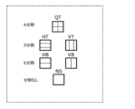
- FIG. 12 is a diagram showing an example of a division pattern.
- Division patterns include, for example, quadrant (QT), in which a block is divided into two in each of the horizontal and vertical directions, and three-division (QT), in which the block is divided into two in the same direction at a ratio of 1:2:1.
- QT quadrant
- QT three-division
- HT or VT two-part division in which the block is divided in the same direction at a 1:1 ratio
- NS no division
- the division pattern does not have a block division direction, and in the case of two divisions and three divisions, the division pattern has division direction information.
- FIG. 13A and 13B are diagrams showing an example of a syntax tree of a division pattern.
- S Split flag
- QT QT flag
- TT TT flag or BT: BT flag
- BT flag BT flag
- the performed determination results may be encoded into a stream according to the encoding order disclosed in the syntax tree shown in FIG. 13A.
- the information is arranged in the order of S, QT, TT, and Ver, but even if the information is arranged in the order of S, QT, Ver, and BT, good.
- S Split flag
- QT QT flag
- BT BT flag or TT: TT flag
- division pattern described here is an example, and a division pattern other than the described division pattern may be used, or only a part of the described division pattern may be used.
- the subtraction unit 104 receives the input from the division unit 102 and subtracts the predicted image (the predicted image input from the prediction control unit 128) from the original image in block units divided by the division unit 102. That is, the subtraction unit 104 calculates the prediction residual of the current block. Then, the subtraction unit 104 outputs the calculated prediction residual to the conversion unit 106.
- the original image is an input signal of the encoding device 100, and is, for example, a signal representing an image of each picture making up a moving image (for example, a luminance (luma) signal and two color difference (chroma) signals).
- a signal representing an image of each picture making up a moving image for example, a luminance (luma) signal and two color difference (chroma) signals.
- the transformer 106 transforms the spatial domain prediction residual into frequency domain transform coefficients, and outputs the transform coefficients to the quantizer 108 .
- the transform unit 106 performs a predetermined discrete cosine transform (DCT) or discrete sine transform (DST) on the prediction residual in the spatial domain, for example.
- DCT discrete cosine transform
- DST discrete sine transform
- the transform unit 106 adaptively selects a transform type from among a plurality of transform types, and converts the predicted residual into transform coefficients using a transform basis function corresponding to the selected transform type. May be converted.
- a transformation is sometimes called EMT (explicit multiple core transform) or AMT (adaptive multiple transform).
- the conversion basis function is sometimes simply called a basis.
- the multiple conversion types include, for example, DCT-II, DCT-V, DCT-VIII, DST-I, and DST-VII. Note that these conversion types may be expressed as DCT2, DCT5, DCT8, DST1, and DST7, respectively.
- FIG. 14 is a table showing transformation basis functions corresponding to each transformation type. In FIG. 14, N indicates the number of input pixels. The selection of a transformation type from among these plurality of transformation types may depend, for example, on the type of prediction (intra prediction, inter prediction, etc.) or on the intra prediction mode.
- EMT flag or AMT flag Information indicating whether to apply such EMT or AMT
- information indicating the selected conversion type are usually signaled at the CU level. Note that the signaling of these information need not be limited to the CU level, but may be at other levels (eg, sequence level, picture level, slice level, brick level, or CTU level).
- the conversion unit 106 may re-convert the conversion coefficients (ie, the conversion result). Such re-transformation is sometimes referred to as AST (adaptive secondary transform) or NSST (non-separable secondary transform). For example, the transform unit 106 re-transforms each sub-block (for example, a 4x4 pixel sub-block) included in the block of transform coefficients corresponding to the intra-prediction residual.
- Information indicating whether to apply NSST and information regarding the transformation matrix used for NSST are usually signaled at the CU level. Note that the signaling of these information need not be limited to the CU level, but may be at other levels (eg, sequence level, picture level, slice level, brick level, or CTU level).
- Separable conversion and non-separable conversion may be applied to the conversion unit 106.
- Separable transformation is a method in which the transformation is performed multiple times by separating each direction by the number of dimensions of the input
- non-separable transformation is a method in which the transformation is performed multiple times in each direction by the number of dimensions of the input. This is a method that treats all dimensions as one-dimensional and performs transformations all at once.
- non-separable transformation if the input is a 4x4 pixel block, it is treated as one array with 16 elements, and 16x16 transformation is performed on that array.
- An example is something that performs a transformation process using a matrix.
- non-separable transformation is a transformation in which a 4x4 pixel input block is treated as one array with 16 elements, and then Givens rotation is performed on the array multiple times ( Hypercube Givens Transform) may also be performed.
- the conversion type of the conversion basis function to be converted into the frequency domain can also be switched depending on the region within the CU.
- An example is SVT (Spatially Varying Transform).
- FIG. 15 is a diagram showing an example of SVT.
- the CU is divided into two in the horizontal or vertical direction, and only one of the regions is converted into the frequency domain.
- the conversion type may be set for each area, and for example, DST7 and DCT8 are used.
- DST7 and DCT8 may be used for the region at position 0.
- DST7 is used for the area at position 1.
- DST7 and DCT8 are used for the region at position 0.
- DST7 is used for the area at position 1.
- the division method may include not only 2 equal divisions but also 4 equal divisions. Further, it is also possible to make it more flexible by encoding information indicating the division method and signaling it in the same way as in CU division. Note that SVT is sometimes referred to as SBT (Sub-block Transform).
- MTS Multiple Transform Selection
- a conversion type such as DST7 or DCT8
- information indicating the selected conversion type may be encoded as index information for each CU.
- IMTS Implicit MTS
- IMTS may be used only for intra-predicted blocks, or may be used for both intra-predicted blocks and inter-predicted blocks.
- each selection process is enabled, or some of them may be selectively enabled. Only the selection process may be enabled. Whether or not each selection process is valid can be identified by flag information in a header such as SPS. For example, if all three selection processes are valid, one of the three selection processes is selected for each CU and orthogonal transformation is performed. Note that the selection process for selectively switching the conversion type may use a selection process different from the above three selection processes, as long as at least one of the following four functions [1] to [4] can be realized. Each of the three selection processes described above may be replaced with another process.
- Function [1] is a function that orthogonally transforms the entire range within the CU and encodes information indicating the transform type used for the transform.
- Function [2] is a function that orthogonally transforms the entire range of the CU and determines the transform type based on a predetermined rule without encoding information indicating the transform type.
- Function [3] is a function that orthogonally transforms a part of the CU and encodes information indicating the transform type used for the transform.
- Function [4] is a function of orthogonally transforming a partial region of the CU and determining the transformation type based on a predetermined rule without encoding information indicating the transformation type used for the transformation.
- whether or not to apply each of MTS, IMTS, and SBT may be determined for each processing unit. For example, whether or not to apply it may be determined on a sequence-by-sequence, picture-by-picture, brick-by-brick, slice-by-slice, CTU-by-CTU, or CU-by-CU basis.
- the tool for selectively switching the conversion type in the present disclosure may be rephrased as a method of adaptively selecting a base to be used in a conversion process, a selection process, or a process of selecting a base. Further, the tool for selectively switching the conversion type may be referred to as a mode for adaptively selecting the conversion type.
- FIG. 16 is a flowchart illustrating an example of processing by the conversion unit 106.
- the transformation unit 106 determines whether or not to perform orthogonal transformation (step St_1).
- the transform unit 106 determines to perform orthogonal transform (Yes in step St_1), it selects a transform type to be used for the orthogonal transform from a plurality of transform types (step St_2).
- the transform unit 106 performs orthogonal transform by applying the selected transform type to the prediction residual of the current block (step St_3).
- the conversion unit 106 outputs information indicating the selected conversion type to the entropy encoding unit 110, thereby encoding the information (Step St_4).
- the transform unit 106 determines that the orthogonal transform is not to be performed (No in step St_1), the transform unit 106 encodes the information by outputting information indicating that the orthogonal transform is not to be performed to the entropy encoding unit 110 ( Step St_5).
- the determination whether or not to perform orthogonal transformation in step St_1 may be determined based on, for example, the size of the transform block, the prediction mode applied to the CU, and the like. Further, the information indicating the transform type used for the orthogonal transform may not be encoded, and the orthogonal transform may be performed using a predefined transform type.
- FIG. 17 is a flowchart showing another example of the processing by the conversion unit 106. Note that, like the example shown in FIG. 16, the example shown in FIG. 17 is an example of orthogonal transformation in which a method of selectively switching the transformation type used for orthogonal transformation is applied.
- the first conversion type group may include DCT2, DST7, and DCT8.
- the second conversion type group may include DCT2.
- the conversion types included in the first conversion type group and the second conversion type group may partially overlap, or may be all different conversion types.
- the converting unit 106 determines whether the converted size is less than or equal to a predetermined value (step Su_1). Here, if it is determined that it is less than or equal to the predetermined value (Yes in step Su_1), the transform unit 106 orthogonally transforms the prediction residual of the current block using the transform type included in the first transform type group (step Su_2 ). Next, the conversion unit 106 outputs information indicating which conversion type to use from among the one or more conversion types included in the first conversion type group to the entropy encoding unit 110, so that the information is encoded (step Su_3).
- the transform unit 106 determines that the transform size is not less than or equal to the predetermined value (No in step Su_1), the transform unit 106 orthogonally transforms the prediction residual of the current block using the second transform type group (step Su_4).
- the information indicating the transformation type used for the orthogonal transformation may be information indicating a combination of the transformation type applied in the vertical direction and the transformation type applied in the horizontal direction of the current block.
- the first transform type group may include only one transform type, and the information indicating the transform type used for orthogonal transform does not need to be encoded.
- the second transform type group may include a plurality of transform types, and information indicating the transform type used for the orthogonal transform among the one or more transform types included in the second transform type group is encoded. It's okay.
- the conversion type may be determined based only on the conversion size. Note that the process is not limited to determining whether the transform size is less than or equal to a predetermined value, as long as the transform type to be used for orthogonal transform is determined based on the transform size.
- Quantization section 108 quantizes the transform coefficients output from transform section 106. Specifically, the quantization unit 108 scans a plurality of transform coefficients of the current block in a predetermined scanning order, and quantizes the transform coefficients based on a quantization parameter (QP) corresponding to the scanned transform coefficients. do. Then, the quantization unit 108 outputs a plurality of quantized transform coefficients (hereinafter referred to as quantization coefficients) of the current block to the entropy encoding unit 110 and the inverse quantization unit 112.
- QP quantization parameter
- the predetermined scanning order is the order for quantization/inverse quantization of transform coefficients.
- the predetermined scanning order is defined as ascending order of frequency (order from low frequency to high frequency) or descending order (order from high frequency to low frequency).
- a quantization parameter is a parameter that defines a quantization step (quantization width). For example, if the value of the quantization parameter increases, the quantization step also increases. In other words, as the value of the quantization parameter increases, the error in the quantization coefficient (quantization error) increases.
- a quantization matrix may be used for quantization.
- quantization matrices may be used depending on frequency conversion sizes such as 4x4 and 8x8, prediction modes such as intra prediction and inter prediction, and pixel components such as luminance and chrominance.
- quantization refers to digitizing values sampled at predetermined intervals by associating them with predetermined levels, and in this technical field, expressions such as rounding, rounding, or scaling are used. In some cases.
- the quantization matrix may be encoded, for example, at the sequence level, picture level, slice level, brick level or CTU level.
- the quantization unit 108 scales, for example, a quantization width determined from a quantization parameter etc. for each transform coefficient using the value of the quantization matrix.
- the quantization process performed without using a quantization matrix may be a process of quantizing transform coefficients based on a quantization width determined from a quantization parameter or the like. Note that in quantization processing performed without using a quantization matrix, the quantization width may be multiplied by a predetermined value that is common to all transform coefficients in a block.
- FIG. 18 is a block diagram showing an example of the configuration of the quantization unit 108.
- the quantization unit 108 includes, for example, a differential quantization parameter generation unit 108a, a predictive quantization parameter generation unit 108b, a quantization parameter generation unit 108c, a quantization parameter storage unit 108d, and a quantization processing unit 108e. .
- FIG. 19 is a flowchart showing an example of quantization by the quantization unit 108.
- the quantization unit 108 may perform quantization for each CU based on the flowchart shown in FIG. Specifically, the quantization parameter generation unit 108c determines whether to perform quantization (step Sv_1). Here, if it is determined that quantization is to be performed (Yes in step Sv_1), the quantization parameter generation unit 108c generates a quantization parameter for the current block (step Sv_2), and stores the quantization parameter in the quantization parameter storage unit 108d. (Step Sv_3).
- the quantization processing unit 108e quantizes the transform coefficient of the current block using the quantization parameter generated in step Sv_2 (step Sv_4).
- the predictive quantization parameter generation unit 108b obtains a quantization parameter for a processing unit different from the current block from the quantization parameter storage unit 108d (step Sv_5).
- the predictive quantization parameter generation unit 108b generates a predictive quantization parameter for the current block based on the acquired quantization parameter (step Sv_6).
- the difference quantization parameter generation unit 108a calculates the difference between the quantization parameter of the current block generated by the quantization parameter generation unit 108c and the predictive quantization parameter of the current block generated by the predictive quantization parameter generation unit 108b. is calculated (step Sv_7). By calculating this difference, a difference quantization parameter is generated.
- the difference quantization parameter generation unit 108a outputs the difference quantization parameter to the entropy encoding unit 110 to encode the difference quantization parameter (step Sv_8).
- differential quantization parameter may be encoded at the sequence level, picture level, slice level, brick level, or CTU level.
- initial value of the quantization parameter may be encoded at the sequence level, picture level, slice level, brick level, or CTU level.
- the quantization parameter may be generated using the initial value of the quantization parameter and the difference quantization parameter.
- the quantization unit 108 may include a plurality of quantizers, and may apply dependent quantization in which the transform coefficients are quantized using a quantization method selected from a plurality of quantization methods.
- FIG. 20 is a block diagram illustrating an example of the configuration of entropy encoding section 110.
- the entropy encoding unit 110 generates a stream by performing entropy encoding on the quantization coefficients input from the quantization unit 108 and the prediction parameters input from the prediction parameter generation unit 130.
- CABAC Context-based Adaptive Binary Arithmetic Coding
- the entropy encoding unit 110 includes, for example, a binarization unit 110a, a context control unit 110b, and a binary arithmetic encoding unit 110c.
- the binarization unit 110a performs binarization to convert multi-value signals such as quantization coefficients and prediction parameters into binary signals.
- Binarization methods include, for example, Truncated Rice Binarization, Exponential Golomb codes, Fixed Length Binarization, and the like.
- the context control unit 110b derives a context value according to the characteristics of the syntax element or the surrounding situation, that is, the probability of occurrence of a binary signal. Methods for deriving this context value include, for example, bypass, syntax element reference, upper/left adjacent block reference, hierarchical information reference, and others.
- the binary arithmetic encoding unit 110c performs arithmetic encoding on the binary signal using the derived context value.
- FIG. 21 is a diagram showing the flow of CABAC in the entropy encoding section 110.
- CABAC in the entropy encoding unit 110 is initialized.
- initialization in the binary arithmetic encoding unit 110c and setting of an initial context value are performed.
- the binarization unit 110a and the binary arithmetic coding unit 110c sequentially perform binarization and arithmetic coding on each of the plurality of quantized coefficients of the CTU, for example.
- the context control unit 110b updates the context value every time arithmetic encoding is performed.
- the context control unit 110b saves the context value as post-processing. This saved context value is used, for example, to initialize the context value for the next CTU.
- the dequantization unit 112 dequantizes the quantized coefficients input from the quantization unit 108. Specifically, the dequantization unit 112 dequantizes the quantization coefficients of the current block in a predetermined scanning order. Then, the inverse quantization unit 112 outputs the inverse quantized transform coefficients of the current block to the inverse transform unit 114.
- the inverse transformer 114 restores the prediction residual by inversely transforming the transform coefficients input from the inverse quantizer 112. Specifically, the inverse transform unit 114 restores the prediction residual of the current block by performing an inverse transform corresponding to the transform by the transform unit 106 on the transform coefficients. Then, the inverse transformer 114 outputs the restored prediction residual to the adder 116.
- the restored prediction residual usually has information lost due to quantization, so it does not match the prediction error calculated by the subtraction unit 104. That is, the restored prediction residual usually includes a quantization error.
- the addition unit 116 reconstructs the current block by adding the prediction residual input from the inverse transformation unit 114 and the predicted image input from the prediction control unit 128. As a result, a reconstructed image is generated. Addition section 116 then outputs the reconstructed image to block memory 118 and loop filter section 120.
- the block memory 118 is, for example, a storage unit for storing blocks in the current picture that are referenced in intra prediction. Specifically, block memory 118 stores the reconstructed image output from adder 116.
- the frame memory 122 is, for example, a storage unit for storing reference pictures used for inter prediction, and is sometimes called a frame buffer. Specifically, the frame memory 122 stores the reconstructed image filtered by the loop filter unit 120.
- the loop filter section 120 performs loop filter processing on the reconstructed image output from the addition section 116 and outputs the filtered reconstructed image to the frame memory 122.
- a loop filter is a filter (in-loop filter) used within the encoding loop, and includes, for example, an adaptive loop filter (ALF), a deblocking filter (DF or DBF), and a sample adaptive offset (SAO). .
- ALF adaptive loop filter
- DF or DBF deblocking filter
- SAO sample adaptive offset
- FIG. 22 is a block diagram showing an example of the configuration of the loop filter section 120.
- the loop filter section 120 includes a deblocking filter processing section 120a, an SAO processing section 120b, and an ALF processing section 120c.
- the deblocking filter processing unit 120a performs the above-described deblocking filter processing on the reconstructed image.
- the SAO processing unit 120b performs the above-described SAO processing on the reconstructed image after the deblocking filter processing.
- the ALF processing unit 120c applies the above-mentioned ALF processing to the reconstructed image after the SAO processing. Details of the ALF and deblocking filter will be described later.
- SAO processing is a process that improves image quality by reducing ringing (a phenomenon in which pixel values are distorted in a wavy manner around edges) and correcting deviations in pixel values.
- This SAO processing includes, for example, edge offset processing and band offset processing.
- the loop filter section 120 does not need to include all of the processing sections disclosed in FIG. 22, and may include only some of the processing sections. Further, the loop filter unit 120 may be configured to perform each of the above-described processes in a different order from the process order disclosed in FIG. 22.
- Loop filter section > Adaptive loop filter In ALF, a least squares error filter is applied to remove coding distortion, and for example, for each 2x2 pixel subblock within the current block, based on the direction and activity of the local gradient. One filter selected from the plurality of filters is applied.
- a subblock for example, a 2x2 pixel subblock
- a plurality of classes for example, 15 or 25 classes. Classification of subblocks is performed, for example, based on the direction and activity of the gradient.
- the sub-blocks are classified into a plurality of classes.
- the gradient direction value D is derived, for example, by comparing gradients in multiple directions (eg, horizontal, vertical, and two diagonal directions). Further, the activation value A of the gradient is derived, for example, by adding gradients in a plurality of directions and quantizing the addition result.
- a filter for the sub-block is determined from among the plurality of filters.
- a circularly symmetrical shape is used as the shape of the filter used in ALF.
- 23A to 23C are diagrams showing a plurality of examples of filter shapes used in ALF.
- Figure 23A shows a 5x5 diamond shaped filter
- Figure 23B shows a 7x7 diamond shaped filter
- Figure 23C shows a 9x9 diamond shaped filter.
- Information indicating the shape of the filter is typically signaled at the picture level. Note that the signalization of information indicating the shape of the filter does not need to be limited to the picture level, and may be at other levels (eg, sequence level, slice level, brick level, CTU level, or CU level).
- the on/off of ALF may be determined at the picture level or CU level, for example. For example, regarding brightness, it may be determined whether to apply ALF at the CU level, and regarding color difference, it may be determined whether to apply ALF at the picture level.
- Information indicating whether the ALF is on or off is usually signaled at the picture level or CU level. Note that the signaling of information indicating on/off of ALF need not be limited to the picture level or CU level, and may be signaled at other levels (for example, sequence level, slice level, brick level, or CTU level). good.
- one filter is selected from the plurality of filters and the ALF processing is performed on the sub-block.
- the coefficient set of coefficients used by that filter is typically signaled at the picture level. Note that the signaling of coefficient sets need not be limited to the picture level, and may be at other levels (eg, sequence level, slice level, brick level, CTU level, CU level, or subblock level).
- FIG. 23D is a diagram showing an example in which the Y sample (first component) is used for Cb CCALF and Cr CCALF (multiple components different from the first component).
- FIG. 23E shows a diamond shaped filter.
- CC-ALF operates by applying a linear diamond-shaped filter (FIGS. 23D, 23E) to the luminance channel of each chrominance component.
- the filter coefficients are sent in APS, scaled by a factor of 2 ⁇ 10, and rounded for fixed point representation.
- Filter application is controlled by variable block sizes and signaled by context-encoded flags received for each block of samples.
- the block size and CC-ALF enable flag are received at the slice level for each chroma component.
- the syntax and semantics of CC-ALF are provided in the Appendix. Block sizes of 16x16, 32x32, 64x64, and 128x128 (in chrominance samples) are supported for contributions.
- FIG. 23F is a diagram showing an example of JC-CCALF.
- FIG. 23G is a diagram illustrating an example of weight_index candidates for JC-CCALF.
- JC-CCALF One example of JC-CCALF is to use only one CCALF filter to produce one CCALF filter output as a color difference adjustment signal for only one color component, and to generate an appropriately weighted version of the same color difference adjustment signal. Apply to other color components. In this way, the complexity of existing CCALF is roughly halved.
- the weight value is encoded into a sign flag and a weight index.
- the weight index (denoted weight_index) is encoded into 3 bits and specifies the size of the JC-CCALF weight JcCcWeight. It cannot be the same as 0.
- the size of JcCcWeight is determined as follows.
- JcCcWeight is equal to 4/(weight_index-4).
- Block-level on/off control of ALF filtering for Cb and Cr is separate. This is the same as CCALF, where two separate sets of block-level on/off control flags are encoded.
- the on/off control block sizes of Cb and Cr are the same, so only one block size variable is encoded.
- loop filter unit 120 reduces distortion occurring at block boundaries by performing filter processing on block boundaries of the reconstructed image.
- FIG. 24 is a block diagram showing an example of a detailed configuration of the deblocking filter processing section 120a.
- the deblocking filter processing unit 120a includes, for example, a boundary determination unit 1201, a filter determination unit 1203, a filter processing unit 1205, a processing determination unit 1208, a filter characteristic determination unit 1207, and switches 1202, 1204, and 1206. Be prepared.
- the boundary determination unit 1201 determines whether a pixel to be subjected to deblocking filter processing (that is, a target pixel) exists near a block boundary. Then, the boundary determining unit 1201 outputs the determination result to the switch 1202 and the processing determining unit 1208.
- the switch 1202 If the boundary determination unit 1201 determines that the target pixel exists near the block boundary, the switch 1202 outputs the image before filter processing to the switch 1204. Conversely, when the boundary determination unit 1201 determines that the target pixel is not present near the block boundary, the switch 1202 outputs the image before filter processing to the switch 1206.
- the image before filter processing is an image consisting of a target pixel and at least one peripheral pixel around the target pixel.
- the filter determination unit 1203 determines whether to perform deblocking filter processing on the target pixel based on the pixel value of at least one peripheral pixel around the target pixel. Filter determination section 1203 then outputs the determination result to switch 1204 and processing determination section 1208.
- the switch 1204 When the filter determination unit 1203 determines that deblocking filter processing is to be performed on the target pixel, the switch 1204 outputs the unfiltered image acquired via the switch 1202 to the filter processing unit 1205. Conversely, when the filter determination unit 1203 determines that the target pixel is not subjected to deblocking filter processing, the switch 1204 outputs the image before filter processing acquired via the switch 1202 to the switch 1206.
- the filter processing unit 1205 When the filter processing unit 1205 acquires the image before filter processing via the switches 1202 and 1204, the filter processing unit 1205 applies deblocking filter processing having the filter characteristics determined by the filter characteristic determination unit 1207 to the target pixel. Execute. Then, the filter processing unit 1205 outputs the filtered pixels to the switch 1206.
- the switch 1206 selectively outputs pixels that have not been subjected to deblocking filter processing and pixels that have been subjected to deblocking filter processing by the filter processing section 1205 in accordance with the control by the processing determining section 1208.
- the processing determination unit 1208 controls the switch 1206 based on the determination results of the boundary determination unit 1201 and the filter determination unit 1203. In other words, when the processing determination unit 1208 determines that the target pixel exists near the block boundary by the boundary determination unit 1201 and the filter determination unit 1203 determines that the target pixel is to be subjected to deblocking filter processing. In this case, the deblocking filtered pixels are output from the switch 1206. In addition, in cases other than the above, the processing determining unit 1208 causes the switch 1206 to output pixels that have not been subjected to deblocking filter processing. By repeatedly outputting pixels in this manner, a filtered image is output from the switch 1206. Note that the configuration shown in FIG. 24 is an example of the configuration of the deblocking filter processing section 120a, and the deblocking filter processing section 120a may have other configurations.
- FIG. 25 is a diagram showing an example of a deblocking filter having filter characteristics that are symmetrical about block boundaries.
- a strong filter and a weak filter is selected using a pixel value and a quantization parameter.
- the strong filter as shown in FIG. 25, when pixels p0 to p2 and pixels q0 to q2 exist on both sides of a block boundary, the pixel value of each pixel q0 to q2 is calculated using the following formula. By doing so, the pixel values are changed to q'0 to q'2.
- p0 to p2 and q0 to q2 are the pixel values of pixels p0 to p2 and pixels q0 to q2, respectively.
- q3 is the pixel value of pixel q3 adjacent to pixel q2 on the opposite side of the block boundary.
- the coefficient by which the pixel value of each pixel used for deblocking filter processing is multiplied is the filter coefficient.
- clipping processing may be performed so that the pixel value after the calculation does not change beyond a threshold value.
- the pixel value after the calculation according to the above formula is clipped to "the pixel value before the calculation ⁇ 2 ⁇ threshold" using the threshold determined from the quantization parameter. This can prevent excessive smoothing.
- FIG. 26 is a diagram for explaining an example of block boundaries on which deblocking filter processing is performed.
- FIG. 27 is a diagram showing an example of BS values.
- the block boundaries on which the deblocking filtering process is performed are, for example, the boundaries of the CU, PU, or TU of an 8 ⁇ 8 pixel block as shown in FIG.
- Deblocking filter processing is performed, for example, in units of four rows or four columns.
- Bs Band Strength
- Deblocking filter processing for color difference signals is performed when the Bs value is 2.
- Deblocking filter processing on the luminance signal is performed when the Bs value is 1 or more and a predetermined condition is satisfied. Note that the conditions for determining the Bs value are not limited to those shown in FIG. 27, and may be determined based on other parameters.
- FIG. 28 is a flowchart illustrating an example of processing performed by the prediction unit of the encoding device 100.
- the prediction unit includes all or some of the components of the intra prediction unit 124, the inter prediction unit 126, and the prediction control unit 128.
- the prediction processing unit includes, for example, an intra prediction unit 124 and an inter prediction unit 126.
- the prediction unit generates a predicted image of the current block (step Sb_1).
- the predicted image includes, for example, an intra predicted image (intra predicted signal) or an inter predicted image (inter predicted signal).
- the prediction unit generates a prediction image that has already been obtained by generating a prediction image for other blocks, generating a prediction residual, generating a quantization coefficient, restoring the prediction residual, and adding the prediction images.
- a predicted image of the current block is generated using the reconstructed image.
- the reconstructed image may be, for example, an image of a reference picture, or an image of a coded block (i.e., another block mentioned above) in the current picture, which is a picture that includes the current block. .
- the coded blocks in the current picture are, for example, adjacent blocks to the current block.
- FIG. 29 is a flowchart showing another example of the processing performed by the prediction unit of the encoding device 100.
- the prediction unit generates a predicted image using the first method (step Sc_1a), generates a predicted image using the second method (step Sc_1b), and generates a predicted image using the third method (step Sc_1c).
- the first method, second method, and third method are mutually different methods for generating a predicted image, and are, for example, an inter prediction method, an intra prediction method, and other prediction methods. There may be. These prediction methods may use the above-described reconstructed images.
- the prediction unit evaluates the predicted images generated in each of steps Sc_1a, Sc_1b, and Sc_1c (step Sc_2). For example, the prediction unit calculates the cost C for the predicted images generated in each of steps Sc_1a, Sc_1b, and Sc_1c, and evaluates the predicted images by comparing the costs C of the predicted images. .
- D is the coding distortion of the predicted image, and is expressed, for example, by the sum of absolute differences between the pixel values of the current block and the pixel values of the predicted image.
- R is the bit rate of the stream.
- ⁇ is, for example, a Lagrangian undetermined multiplier.
- the prediction unit selects any one of the predicted images generated in each of steps Sc_1a, Sc_1b, and Sc_1c (step Sc_3). That is, the prediction unit selects a method or mode for obtaining a final predicted image. For example, the prediction unit selects the predicted image with the smallest cost C based on the costs C calculated for those predicted images. Alternatively, the evaluation in step Sc_2 and the selection of the predicted image in step Sc_3 may be performed based on parameters used in the encoding process.
- the encoding device 100 may signal information for specifying the selected predicted image, method, or mode into a stream. The information may be, for example, a flag.
- the decoding device 200 can generate a predicted image according to the method or mode selected by the encoding device 100 based on the information.
- the prediction unit selects one of the predicted images after generating predicted images using each method.
- the prediction unit may select a method or mode based on the parameters used in the encoding process described above, and generate predicted images according to that method or mode. good.
- the first method and the second method are intra prediction and inter prediction, respectively, and the prediction unit selects the final predicted image for the current block from the predicted images generated according to these prediction methods. You may.
- FIG. 30 is a flowchart showing another example of the processing performed by the prediction unit of the encoding device 100.
- the prediction unit generates a predicted image by intra prediction (step Sd_1a), and generates a predicted image by inter prediction (step Sd_1b).
- a predicted image generated by intra prediction is also referred to as an intra predicted image
- a predicted image generated by inter prediction is also referred to as an inter predicted image.
- the prediction unit evaluates each of the intra-predicted image and the inter-predicted image (step Sd_2).
- the above-mentioned cost C may be used for this evaluation.
- the prediction unit may select the predicted image for which the smallest cost C is calculated from the intra-predicted image and the inter-predicted image as the final predicted image of the current block (step Sd_3). That is, a prediction method or mode for generating a predicted image of the current block is selected.
- the intra prediction unit 124 performs intra prediction (also referred to as intra-picture prediction) of the current block by referring to the blocks in the current picture stored in the block memory 118, thereby generating a predicted image (that is, an intra predicted image) of the current block. generate. Specifically, the intra prediction unit 124 generates an intra prediction image by performing intra prediction with reference to pixel values (for example, brightness values, color difference values) of blocks adjacent to the current block, and predicts the intra prediction image. It is output to the control section 128.
- intra prediction also referred to as intra-picture prediction
- the intra prediction unit 124 performs intra prediction using one of a plurality of predefined intra prediction modes.
- the multiple intra prediction modes typically include one or more non-directional prediction modes and multiple directional prediction modes.
- the one or more non-directional prediction modes may include, for example, H. This includes Planar prediction mode and DC prediction mode defined in the H.265/HEVC standard.
- FIG. 31 is a diagram showing a total of 67 intra prediction modes (2 non-directional prediction modes and 65 directional prediction modes) in intra prediction. Solid arrows indicate H. The dashed arrows represent the 33 directions defined in the H.265/HEVC standard, and the dashed arrows represent the 32 additional directions (the two non-directional prediction modes are not shown in FIG. 31).
- luma blocks may be referenced in intra prediction of chroma blocks. That is, the chrominance component of the current block may be predicted based on the luminance component of the current block.
- Such intra prediction is sometimes called cross-component linear model (CCLM) prediction.
- An intra prediction mode for a chrominance block that refers to such a luminance block (for example, referred to as a CCLM mode) may be added as one of the intra prediction modes for a chrominance block.
- the intra prediction unit 124 may correct the pixel value after intra prediction based on the gradient of the reference pixel in the horizontal/vertical direction. Intra prediction accompanied by such correction is sometimes called position dependent intra prediction combination (PDPC). Information indicating whether PDPC is applied (for example, called a PDPC flag) is usually signaled at the CU level. Note that the signaling of this information need not be limited to the CU level, but may be at other levels (eg, sequence level, picture level, slice level, brick level or CTU level).
- FIG. 32 is a flowchart illustrating an example of processing by the intra prediction unit 124.
- the intra prediction unit 124 selects one intra prediction mode from a plurality of intra prediction modes (step Sw_1). Then, the intra prediction unit 124 generates a predicted image according to the selected intra prediction mode (step Sw_2). Next, the intra prediction unit 124 determines MPM (Most Probable Modes) (step Sw_3).
- MPM consists of, for example, six intra prediction modes. Two of the six intra prediction modes may be Planar prediction mode and DC prediction mode, and the remaining four modes may be directional prediction modes. Then, the intra prediction unit 124 determines whether the intra prediction mode selected in step Sw_1 is included in the MPM (step Sw_4).
- the intra prediction unit 124 sets the MPM flag to 1 (step Sw_5), and selects the selected intra prediction mode from the MPM. (Step Sw_6). Note that the MPM flag set to 1 and the information indicating its intra prediction mode are each encoded by the entropy encoding unit 110 as prediction parameters.
- the intra prediction unit 124 sets the MPM flag to 0 (step Sw_7). Alternatively, the intra prediction unit 124 does not set the MPM flag. Then, the intra prediction unit 124 generates information indicating the selected intra prediction mode from among the one or more intra prediction modes not included in the MPM (step Sw_8). Note that the MPM flag set to 0 and the information indicating its intra prediction mode are each encoded by the entropy encoding unit 110 as prediction parameters. The information indicating the intra prediction mode indicates any value from 0 to 60, for example.
- the inter prediction unit 126 performs inter prediction (also referred to as inter prediction) of the current block by referring to a reference picture stored in the frame memory 122 that is different from the current picture, thereby generating a predicted image (inter prediction). (predicted image). Inter prediction is performed in units of the current block or current subblock within the current block.
- a subblock is included in a block and is a unit smaller than the block.
- the size of the sub-block may be 4x4 pixels, 8x8 pixels, or any other size.
- the size of subblocks may be switched in units of slices, bricks, pictures, or the like.
- the inter prediction unit 126 performs motion estimation within a reference picture for the current block or current subblock, and finds a reference block or subblock that most closely matches the current block or current subblock. Then, the inter prediction unit 126 obtains motion information (eg, motion vector) that compensates for movement or change from the reference block or subblock to the current block or subblock. The inter prediction unit 126 performs motion compensation (or motion prediction) based on the motion information and generates an inter prediction image of the current block or subblock. The inter prediction unit 126 outputs the generated inter prediction image to the prediction control unit 128.
- motion information eg, motion vector
- the inter prediction unit 126 performs motion compensation (or motion prediction) based on the motion information and generates an inter prediction image of the current block or subblock.
- the inter prediction unit 126 outputs the generated inter prediction image to the prediction control unit 128.
- the motion information used for motion compensation may be signalized as an inter-predicted image in various forms.
- motion vectors may be signaled.
- a difference between a motion vector and a motion vector predictor may be signaled.
- FIG. 33 is a diagram showing an example of each reference picture
- FIG. 34 is a conceptual diagram showing an example of a reference picture list.
- the reference picture list is a list indicating one or more reference pictures stored in the frame memory 122.
- rectangles indicate pictures
- arrows indicate reference relationships between pictures
- the horizontal axis indicates time
- I, P, and B in the rectangles indicate intra-predicted pictures, uni-predicted pictures, and bi-predicted pictures, respectively.
- the number inside the rectangle indicates the decoding order.
- the decoding order of each picture is I0, P1, B2, B3, B4, and the display order of each picture is I0, B3, B2, B4, P1.
- FIG. 33 the decoding order of each picture is I0, P1, B2, B3, B4, and the display order of each picture is I0, B3, B2, B4, P1.
- the reference picture list is a list representing reference picture candidates, and for example, one picture (or slice) may have one or more reference picture lists. For example, if the current picture is a uni-prediction picture, one reference picture list is used, and if the current picture is a bi-prediction picture, two reference picture lists are used.
- picture B3 which is the current picture currPic, has two reference picture lists, the L0 list and the L1 list.
- reference picture candidates for the current picture currPic are I0, P1, and B2, and each reference picture list (ie, L0 list and L1 list) indicates these pictures.
- the inter prediction unit 126 or the prediction control unit 128 specifies which picture in each reference picture list is actually referred to or not using the reference picture index refIdxLx.
- reference pictures P1 and B2 are specified by reference picture indexes refIdxL0 and refIdxL1.
- Such a reference picture list may be generated in sequence units, picture units, slice units, brick units, CTU units, or CU units. Also, among the reference pictures shown in the reference picture list, a reference picture index indicating a reference picture referred to in inter prediction is encoded at the sequence level, picture level, slice level, brick level, CTU level, or CU level. Good too. Further, a common reference picture list may be used in a plurality of inter prediction modes.
- FIG. 35 is a flowchart showing the basic flow of inter prediction.
- the inter prediction unit 126 first generates a predicted image (steps Se_1 to Se_3). Next, the subtraction unit 104 generates the difference between the current block and the predicted image as a prediction residual (step Se_4).
- the inter prediction unit 126 determines the motion vector (MV) of the current block (steps Se_1 and Se_2) and performs motion compensation (step Se_3), thereby generating the predicted image. generate. Further, in determining the MV, the inter prediction unit 126 determines the MV by, for example, selecting a candidate motion vector (candidate MV) (step Se_1) and deriving the MV (step Se_2). The selection of candidate MVs is performed, for example, by the inter prediction unit 126 generating a candidate MV list and selecting at least one candidate MV from the candidate MV list. Note that MVs derived in the past may be added to the candidate MV list as candidate MVs.
- the inter prediction unit 126 further selects at least one candidate MV from at least one candidate MV, and determines the selected at least one candidate MV as the MV of the current block. It's okay.
- the inter prediction unit 126 may determine the MV of the current block for each of the selected at least one candidate MV by searching the area of the reference picture indicated by the candidate MV. Note that searching for this reference picture area may be referred to as motion estimation.
- steps Se_1 to Se_3 are performed by the inter prediction unit 126, but for example, the processing such as step Se_1 or step Se_2 may be performed by other components included in the encoding device 100. .
- a candidate MV list may be created for each process in each inter prediction mode, or a common candidate MV list may be used in multiple inter prediction modes.
- the processes in steps Se_3 and Se_4 correspond to the processes in steps Sa_3 and Sa_4 shown in FIG. 9, respectively.
- the process of step Se_3 corresponds to the process of step Sd_1b in FIG. 30.
- FIG. 36 is a flowchart showing an example of MV derivation.
- the inter prediction unit 126 may derive the MV of the current block in a mode that encodes motion information (for example, MV).
- motion information for example, MV
- motion information may be encoded as a prediction parameter and converted into a signal. That is, encoded motion information is included in the stream.
- the inter prediction unit 126 may derive the MV in a mode in which motion information is not encoded. In this case, motion information is not included in the stream.
- MV derivation modes include normal inter mode, normal merge mode, FRUC mode, and affine mode, which will be described later.
- modes for encoding motion information include normal inter mode, normal merge mode, and affine mode (specifically, affine inter mode and affine merge mode).
- the motion information may include not only MV but also predicted MV selection information, which will be described later.
- modes in which motion information is not encoded include a FRUC mode.
- the inter prediction unit 126 selects a mode for deriving the MV of the current block from these multiple modes, and derives the MV of the current block using the selected mode.
- FIG. 37 is a flowchart showing another example of MV derivation.
- the inter prediction unit 126 may derive the MV of the current block in a mode of encoding the difference MV.
- the difference MV is encoded as a prediction parameter and converted into a signal.
- the encoded difference MV is included in the stream.
- This difference MV is the difference between the MV of the current block and its predicted MV.
- the predicted MV is a predicted motion vector.
- the inter prediction unit 126 may derive the MV in a mode in which the difference MV is not encoded. In this case, the encoded differential MV is not included in the stream.
- modes for deriving the MV include normal inter, normal merge mode, FRUC mode, and affine mode, which will be described later.
- modes for encoding the difference MV include normal inter mode and affine mode (specifically, affine inter mode).
- modes in which differential MVs are not encoded include FRUC mode, normal merge mode, and affine mode (specifically, affine merge mode).
- the inter prediction unit 126 selects a mode for deriving the MV of the current block from these multiple modes, and derives the MV of the current block using the selected mode.
- FIGS. 38A and 38B are diagrams showing an example of classification of each mode of MV derivation.
- MV derivation modes are roughly classified into three modes depending on whether motion information is encoded and whether differential MV is encoded.
- the three modes are inter mode, merge mode, and frame rate up-conversion (FRUC) mode.
- Inter mode is a mode for performing motion search, and is a mode for encoding motion information and difference MV.
- inter modes include affine inter mode and normal inter mode.
- the merge mode is a mode in which no motion search is performed, and in which MVs are selected from neighboring encoded blocks and the MVs are used to derive the MV of the current block.
- This merge mode is basically a mode in which motion information is encoded and differential MV is not encoded.
- the merge modes include normal merge mode (sometimes called normal merge mode or regular merge mode), MMVD (Merge with Motion Vector Difference) mode, and CIIP (Combined inter merge/intra prediction). ) mode , triangle mode, ATMVP mode, and affine merge mode.
- the difference MV is exceptionally encoded in the MMVD mode among the modes included in the merge mode.
- the above-mentioned affine merge mode and affine inter mode are modes included in the affine mode.
- the affine mode is a mode in which the MV of each of a plurality of sub-blocks constituting the current block is derived as the MV of the current block assuming affine transformation.
- the FRUC mode is a mode in which the MV of the current block is derived by searching between encoded regions, and neither motion information nor differential MV is encoded. Note that details of each of these modes will be described later.
- each mode shown in FIGS. 38A and 38B is an example and is not limited to this.
- the CIIP mode is classified as inter mode.
- the normal inter prediction mode is an inter prediction mode in which the MV of the current block is derived by finding a block similar to the image of the current block from the area of the reference picture indicated by the candidate MV. Further, in this normal inter mode, the difference MV is encoded.
- FIG. 39 is a flowchart illustrating an example of inter prediction in normal inter mode.
- the inter prediction unit 126 first obtains a plurality of candidate MVs for the current block based on information such as MVs of a plurality of encoded blocks temporally or spatially surrounding the current block (step Sg_1). That is, the inter prediction unit 126 creates a candidate MV list.
- the inter prediction unit 126 selects each of the N candidate MVs (N is an integer of 2 or more) as predicted MV candidates from among the plurality of candidate MVs obtained in step Sg_1, and assigns them to a predetermined priority order. (Step Sg_2). Note that the priority order is determined in advance for each of the N candidate MVs.
- the inter prediction unit 126 selects one predicted MV candidate from among the N predicted MV candidates as the predicted MV of the current block (step Sg_3). At this time, the inter prediction unit 126 encodes predicted MV selection information for identifying the selected predicted MV into a stream. That is, the inter prediction unit 126 outputs the predicted MV selection information as a prediction parameter to the entropy encoding unit 110 via the prediction parameter generation unit 130.
- the inter prediction unit 126 refers to the encoded reference picture and derives the MV of the current block (step Sg_4). At this time, the inter prediction unit 126 further encodes the difference value between the derived MV and the predicted MV into a stream as a difference MV. That is, the inter prediction unit 126 outputs the difference MV as a prediction parameter to the entropy encoding unit 110 via the prediction parameter generation unit 130.
- the encoded reference picture is a picture consisting of a plurality of blocks that has been reconstructed after encoding.
- the inter prediction unit 126 generates a predicted image of the current block by performing motion compensation on the current block using the derived MV and the encoded reference picture (step Sg_5).
- the processes of steps Sg_1 to Sg_5 are executed for each block. For example, when steps Sg_1 to Sg_5 are executed for each of all blocks included in a slice, inter prediction using normal inter mode for that slice ends. Moreover, when the processes of steps Sg_1 to Sg_5 are executed for each of all blocks included in a picture, inter prediction using normal inter mode for that picture is completed. Note that the processing in steps Sg_1 to Sg_5 is not executed for all blocks included in a slice, but when executed for some blocks, inter prediction using normal inter mode for that slice is completed. It's okay. Similarly, when the processes of steps Sg_1 to Sg_5 are executed for some blocks included in a picture, inter prediction using normal inter mode for that picture may be completed.
- the predicted image is the above-mentioned inter predicted signal. Furthermore, information included in the encoded signal and indicating the inter prediction mode (normal inter mode in the above example) used to generate the predicted image is encoded, for example, as a prediction parameter.
- the candidate MV list may be used in common with lists used in other modes. Further, the processing related to the candidate MV list may be applied to the processing related to the list used in other modes. Processing related to this candidate MV list includes, for example, extracting or selecting candidate MVs from the candidate MV list, rearranging candidate MVs, or deleting candidate MVs.
- the normal merge mode is an inter prediction mode in which a candidate MV is selected from the candidate MV list as the MV of the current block, thereby deriving the MV.
- the normal merge mode is a merge mode in a narrow sense, and is sometimes simply called a merge mode.
- a normal merge mode and a merge mode are distinguished, and the merge mode is used in a broad sense.
- FIG. 40 is a flowchart illustrating an example of inter prediction in normal merge mode.
- the inter prediction unit 126 first obtains a plurality of candidate MVs for the current block based on information such as MVs of a plurality of encoded blocks temporally or spatially surrounding the current block (step Sh_1). That is, the inter prediction unit 126 creates a candidate MV list.
- the inter prediction unit 126 derives the MV of the current block by selecting one candidate MV from the plurality of candidate MVs obtained in step Sh_1 (step Sh_2). At this time, the inter prediction unit 126 encodes MV selection information for identifying the selected candidate MV into a stream. That is, the inter prediction unit 126 outputs the MV selection information as a prediction parameter to the entropy encoding unit 110 via the prediction parameter generation unit 130.
- the inter prediction unit 126 generates a predicted image of the current block by performing motion compensation on the current block using the derived MV and the encoded reference picture (step Sh_3).
- the processes of steps Sh_1 to Sh_3 are executed for each block, for example. For example, when steps Sh_1 to Sh_3 are executed for each of all blocks included in a slice, inter prediction using the normal merge mode for that slice ends. Further, when the processes of steps Sh_1 to Sh_3 are executed for each of all blocks included in a picture, inter prediction using the normal merge mode for that picture ends. Note that the processing in steps Sh_1 to Sh_3 is not executed for all blocks included in a slice, but when executed for some blocks, inter prediction using normal merge mode for that slice is completed. It's okay. Similarly, when the processes of steps Sh_1 to Sh_3 are executed for some blocks included in a picture, inter prediction using normal merge mode for that picture may be completed.
- information included in the stream indicating the inter prediction mode (normal merge mode in the above example) used to generate the predicted image is encoded as a prediction parameter, for example.
- FIG. 41 is a diagram for explaining an example of MV derivation processing for the current picture in normal merge mode.
- the inter prediction unit 126 generates a candidate MV list in which candidate MVs are registered.
- Candidate MVs include spatially adjacent candidate MVs that are MVs held by multiple coded blocks spatially located around the current block, and MVs held by nearby blocks that are the projections of the position of the current block in the coded reference picture.
- There are temporally adjacent candidate MV that is combined candidate MV that is MV that is generated by combining the MV values of spatially adjacent candidate MV and temporally adjacent candidate MV, and zero candidate MV that is MV whose value is zero.
- the inter prediction unit 126 selects one candidate MV from among the plurality of candidate MVs registered in the candidate MV list, and determines that one candidate MV as the MV of the current block.
- the entropy encoding unit 110 describes merge_idx, which is a signal indicating which candidate MV has been selected, in the stream and encodes it.
- the candidate MVs registered in the candidate MV list explained in FIG. 41 are just examples, and the number of candidate MVs registered in the candidate MV list explained in FIG.
- the structure may include additional candidate MVs other than the candidate MV types shown in the figure.
- the final MV may be determined by performing DMVR (dynamic motion vector refreshing), which will be described later, using the MV of the current block derived in the normal merge mode.
- DMVR dynamic motion vector refreshing
- the difference MV is not encoded, but in the MMVD mode, the difference MV is encoded.
- one candidate MV is selected from the candidate MV list as in the normal merge mode, but the difference MV is encoded.
- Such MMVD may be classified into a merge mode together with a normal merge mode, as shown in FIG. 38B.
- the differential MV in MMVD mode does not have to be the same as the differential MV used in inter mode. For example, deriving differential MV in MMVD mode requires less processing than deriving differential MV in inter mode. It may be a small process.
- a CIIP (Combined inter merge/intra prediction) mode may be performed in which a predicted image generated by inter prediction and a predicted image generated by intra prediction are superimposed to generate a predicted image of the current block.
- merge_idx is MV selection information.
- FIG. 42 is a diagram for explaining an example of MV derivation processing for the current picture in HMVP mode.
- the MV of the current block is determined by selecting one candidate MV from a candidate MV list generated with reference to the encoded block (eg, CU).
- a candidate MV list generated with reference to the encoded block (eg, CU).
- other candidate MVs may be registered in the candidate MV list.
- the mode in which such other candidate MVs are registered is called HMVP mode.
- HMVP mode apart from the candidate MV list in normal merge mode, candidate MVs are managed using a FIFO (First-In First-Out) buffer for HMVP.
- FIFO First-In First-Out
- the FIFO buffer stores motion information such as MV of blocks processed in the past in order from newest to newest.
- the MV of the newest block i.e., the most recently processed CU
- the MV of the oldest block in the FIFO buffer i.e., The MV of the earliest processed CU
- HMVP1 is the MV of the newest block
- HMVP5 is the MV of the oldest block.
- the inter prediction unit 126 sequentially selects each MV managed in the FIFO buffer, starting from HMVP1, if the MV is different from all the candidate MVs already registered in the normal merge mode candidate MV list. Check if there is. If the inter prediction unit 126 determines that the MV is different from all candidate MVs, it may add the MV managed in the FIFO buffer to the normal merge mode candidate MV list as a candidate MV. At this time, the number of candidate MVs registered from the FIFO buffer may be one or multiple.
- HMVP mode By using the HMVP mode in this way, it is possible to add not only the MVs of blocks spatially or temporally adjacent to the current block, but also the MVs of blocks processed in the past to candidates. As a result, the variation of normal merge mode candidate MVs is expanded, which increases the possibility that encoding efficiency can be improved.
- the above-mentioned MV may be motion information.
- the information stored in the candidate MV list and the FIFO buffer may include not only the MV value but also information on the picture to be referenced, the direction and number of pictures to be referenced, and the like.
- the above-mentioned block is, for example, a CU.
- the candidate MV list and FIFO buffer in FIG. 42 are just examples, and the candidate MV list and FIFO buffer may be a list or buffer of a different size from that in FIG. 42, or the candidate MVs may be registered in a different order from that in FIG. It may be a configuration. Further, the processing described here is common to both encoding device 100 and decoding device 200.
- HMVP mode can also be applied to modes other than normal merge mode.
- motion information such as MVs of blocks processed in the affine mode in the past may be stored in a FIFO buffer in order from the newest to the latest, and may be used as candidate MVs.
- a mode in which the HMVP mode is applied to an affine mode may be called a history affine mode.
- the motion information may be derived on the decoding device 200 side without being converted into a signal from the encoding device 100 side.
- motion information may be derived by performing motion search on the decoding device 200 side.
- motion search is performed without using the pixel values of the current block.
- Modes in which motion search is performed on the decoding device 200 side include a FRUC (frame rate up-conversion) mode and a PMMVD (pattern matched motion vector derivation) mode.
- FRUC processing is shown in FIG. 43.
- a list indicating these MVs as candidate MVs i.e., a candidate MV list, which is a candidate MV in normal merge mode
- a candidate MV list which is a candidate MV in normal merge mode
- the best candidate MV is selected from among the plurality of candidate MVs registered in the candidate MV list (step Si_2). For example, an evaluation value of each candidate MV included in the candidate MV list is calculated, and one candidate MV is selected as the best candidate MV based on the evaluation value.
- the MV for the current block is derived (step Si_4).
- the selected best candidate MV is directly derived as the MV for the current block.
- the MV for the current block may be derived by performing pattern matching in the surrounding area of the position in the reference picture corresponding to the selected best candidate MV. That is, a search is performed using pattern matching in the reference picture and the evaluation value for the area around the best candidate MV, and if there is an MV with a good evaluation value, the best candidate MV is added to that MV. It may be updated to make it the final MV of the current block. There is no need to update to an MV with a better evaluation value.
- the inter prediction unit 126 generates a predicted image of the current block by performing motion compensation on the current block using the derived MV and the encoded reference picture (step Si_5).
- the processes of steps Si_1 to Si_5 are executed for each block, for example. For example, when steps Si_1 to Si_5 are executed for each of all blocks included in a slice, inter prediction using the FRUC mode for that slice ends. Further, when the processes of steps Si_1 to Si_5 are executed for each of all blocks included in a picture, inter prediction using the FRUC mode for that picture ends. Note that the processing in steps Si_1 to Si_5 is not executed for all blocks included in a slice, but when executed for some blocks, the inter prediction using FRUC mode for that slice is completed. Good too. Similarly, when the processes of steps Si_1 to Si_5 are executed for some blocks included in a picture, inter prediction using FRUC mode for that picture may be completed.
- Processing may be performed in units of sub-blocks in the same manner as in the units of blocks described above.
- the evaluation value may be calculated by various methods. For example, a reconstructed image of a region within a reference picture corresponding to the MV and a predetermined region (for example, the region may be a region of another reference picture or a region of an adjacent block of the current picture, as shown below). Compare the reconstructed image of Then, the difference between the pixel values of the two reconstructed images may be calculated and used as the MV evaluation value. Note that the evaluation value may be calculated using information other than the difference value.
- one candidate MV included in a candidate MV list (also referred to as a merge list) is selected as a starting point for a search by pattern matching.
- pattern matching first pattern matching or second pattern matching may be used.
- the first pattern matching and the second pattern matching may be referred to as bilateral matching and template matching, respectively.
- MV derivation > FRUC > Bilateral matching In the first pattern matching, pattern matching is performed between two blocks in two different reference pictures that are along the motion trajectory of the current block. Therefore, in the first pattern matching, a region in another reference picture along the motion trajectory of the current block is used as a predetermined region for calculating the evaluation value of the candidate MV described above.
- FIG. 44 is a diagram for explaining an example of first pattern matching (bilateral matching) between two blocks in two reference pictures along a motion trajectory.
- first pattern matching a pair of two blocks in two different reference pictures (Ref0, Ref1) that are along the motion trajectory of the current block (Cur block) is selected.
- Two MVs (MV0, MV1) are derived by searching for the most matching pair. Specifically, for the current block, a reconstructed image at a specified position in the first encoded reference picture (Ref0) specified by a candidate MV, and a symmetric MV obtained by scaling the candidate MV at the display time interval.
- the difference between the reconstructed image and the specified position in the second encoded reference picture (Ref1) specified by is derived, and an evaluation value is calculated using the obtained difference value.
- the candidate MV with the best evaluation value among the plurality of candidate MVs may be selected as the best candidate MV.
- the MVs (MV0, MV1) pointing to two reference blocks are defined as the temporal distance ( TD0, TD1).
- the temporal distance TD0, TD1
- MV Derivation > FRUC > Template Matching In the second pattern matching (template matching), pattern matching is performed between a template in the current picture (blocks adjacent to the current block in the current picture (e.g. upper and/or left adjacent blocks)) and blocks in the reference picture. It will be done. Therefore, in the second pattern matching, a block adjacent to the current block in the current picture is used as a predetermined area for calculating the evaluation value of the candidate MV described above.
- FIG. 45 is a diagram for explaining an example of pattern matching (template matching) between a template in the current picture and a block in the reference picture.
- the current block is searched in the reference picture (Ref0) for the block that most matches the block adjacent to the current block (Cur block) in the current picture (Cur Pic).
- MV of is derived. Specifically, for the current block, the reconstructed image of the left adjacent and/or upper adjacent encoded area and the equivalent image in the encoded reference picture (Ref0) specified by the candidate MV. A difference between the position and the reconstructed image is derived, and an evaluation value is calculated using the obtained difference value. The candidate MV with the best evaluation value among the plurality of candidate MVs may be selected as the best candidate MV.
- Information indicating whether to apply such a FRUC mode may be signaled at the CU level. Furthermore, when the FRUC mode is applied (for example, when the FRUC flag is true), information indicating an applicable pattern matching method (first pattern matching or second pattern matching) may be signaled at the CU level. . Note that the signaling of these information does not need to be limited to the CU level, and may be at other levels (e.g., sequence level, picture level, slice level, brick level, CTU level, or subblock level). .
- the affine mode is a mode in which an MV is generated using affine transformation, and for example, the MV may be derived in subblock units based on the MVs of a plurality of adjacent blocks. This mode is sometimes referred to as affine motion compensation prediction mode.
- FIG. 46A is a diagram for explaining an example of deriving MV in sub-block units based on MVs of a plurality of adjacent blocks.
- the current block includes, for example, a subblock consisting of 16 4x4 pixels.
- the motion vector v 0 of the upper left corner control point of the current block is derived based on the MV of the adjacent block
- the motion vector v 1 of the upper right corner control point of the current block is derived based on the MV of the adjacent sub-block. derived.
- equation (1A) the two motion vectors v 0 and v 1 are projected to derive the motion vector (v x , v y ) of each subblock within the current block.
- x and y indicate the horizontal and vertical positions of the sub-block, respectively, and w indicates a predetermined weighting factor.
- Information indicating such an affine mode may be signaled at the CU level.
- an affine flag may be signaled at the CU level. Note that the signaling of information indicating this affine mode does not need to be limited to the CU level, and may be signaled at other levels (e.g., sequence level, picture level, slice level, brick level, CTU level, or subblock level). It's okay.
- affine modes may include several modes in which the methods for deriving the MVs of the upper left and upper right corner control points are different.
- affine inter also referred to as affine normal inter
- affine merge mode there are two affine modes: affine inter (also referred to as affine merge mode.
- FIG. 46B is a diagram for explaining an example of deriving MV in sub-block units in affine mode using three control points.
- the current block includes, for example, a subblock consisting of 16 4x4 pixels.
- the motion vector v 0 of the upper left corner control point of the current block is derived based on the MV of the adjacent block.
- the motion vector v 1 of the upper right corner control point of the current block is derived based on the MV of the adjacent block
- the motion vector v 2 of the lower left corner control point of the current block is derived based on the MV of the adjacent block.
- the motion vectors (v x , v y ) of each subblock within the current block are derived by projecting the three motion vectors v 0 , v 1 , and v 2 using the following equation (1B).
- x and y indicate the horizontal and vertical positions of the sub-block center, respectively, and w and h indicate predetermined weighting coefficients.
- w may indicate the width of the current block, and h may indicate the height of the current block.
- Affine modes using mutually different numbers of control points may be switched and signaled at the CU level.
- information indicating the number of affine mode control points used at the CU level may be signaled at other levels (e.g., sequence level, picture level, slice level, brick level, CTU level, or subblock level). good.
- such an affine mode having three control points may include several modes in which the methods for deriving the MVs of the upper left, upper right, and lower left corner control points are different.
- the affine mode with three control points has two modes: affine inter mode and affine merge mode, similar to the above-described affine mode with two control points.
- each sub-block included in the current block is not limited to 4x4 pixels, and may be any other size.
- the size of each sub-block may be 8x8 pixels.
- FIG. 47A, FIG. 47B, and FIG. 47C are conceptual diagrams for explaining an example of MV derivation of control points in affine mode.
- encoded blocks A (left), block B (top), block C (top right), block D (bottom left), and block E (top left) adjacent to the current block are calculated based on a plurality of MVs corresponding to blocks encoded in affine mode.
- the encoded blocks are examined in the following order: block A (left), block B (top), block C (top right), block D (bottom left), and block E (top left), and the blocks are examined in affine mode.
- the first valid block encoded is identified. Based on the plurality of MVs corresponding to this identified block, the MV of the control point of the current block is calculated.
- the upper left corner, upper right corner of the encoded block including block A And motion vectors v 3 , v 4 and v 5 projected onto the lower left corner position are derived. Then, from the derived motion vectors v 3 , v 4 and v 5 , the motion vector v 0 of the upper left corner control point, the motion vector v 1 of the upper right corner control point, and the motion vector v of the lower left corner control point of the current block. 2 is calculated.
- the MV derivation method shown in FIGS. 47A to 47C may be used to derive the MV of each control point of the current block in step Sk_1 shown in FIG. 50 described later, or in step Sj_1 shown in FIG. 51 described later. may be used to derive the predicted MV of each control point of the current block.
- FIGS. 48A and 48B are conceptual diagrams for explaining another example of deriving control points MV in affine mode.
- FIG. 48A is a diagram for explaining an affine mode with two control points.
- the MV selected from the MVs of encoded blocks A, B, and C adjacent to the current block is the motion vector v of the upper left corner control point of the current block. Used as 0 .
- the MV selected from the respective MVs of encoded blocks D and E adjacent to the current block is used as the motion vector v 1 of the upper right corner control point of the current block.
- FIG. 48B is a diagram for explaining an affine mode having three control points.
- the MV selected from the MVs of encoded blocks A, B, and C adjacent to the current block is the motion vector v of the upper left corner control point of the current block. Used as 0 .
- the MV selected from the respective MVs of encoded blocks D and E adjacent to the current block is used as the motion vector v 1 of the upper right corner control point of the current block.
- the MV selected from the respective MVs of encoded blocks F and G adjacent to the current block is used as the motion vector v2 of the lower left corner control point of the current block.
- the MV derivation method shown in FIGS. 48A and 48B may be used for deriving the MV of each control point of the current block in step Sk_1 shown in FIG. 50, which will be described later, or in step Sj_1 of FIG. It may be used to derive the predicted MV of each control point of the current block.
- the number of control points may be different between the encoded block and the current block.
- FIGS. 49A and 49B are conceptual diagrams for explaining an example of a method for deriving MV of control points when the number of control points is different between the encoded block and the current block.
- the current block has three control points at the upper left corner, the upper right corner, and the lower left corner, and the block A adjacent to the left of the current block is encoded in affine mode with two control points. has been done.
- motion vectors v 3 and v 4 projected onto the upper left corner and upper right corner of the encoded block including block A are derived.
- the motion vector v 0 of the upper left corner control point and the motion vector v 1 of the upper right corner control point of the current block are calculated from the derived motion vectors v 3 and v 4 .
- the motion vector v 2 of the lower left corner control point is calculated from the derived motion vectors v 0 and v 1 .
- the current block has two control points at the upper left corner and the upper right corner, and the block A adjacent to the left of the current block is encoded in affine mode with three control points. .
- motion vectors v 3 , v 4 and v 5 projected onto the upper left corner, upper right corner and lower left corner of the encoded block including block A are derived.
- the motion vector v 0 of the upper left corner control point and the motion vector v 1 of the upper right corner control point of the current block are calculated from the derived motion vectors v 3 , v 4 and v 5 .
- the MV derivation method shown in FIGS. 49A and 49B may be used for deriving the MV of each control point of the current block in step Sk_1 shown in FIG. 50, which will be described later, or in step Sj_1 of FIG. It may be used to derive the predicted MV of each control point of the current block.
- FIG. 50 is a flowchart illustrating an example of affine merge mode.
- the inter prediction unit 126 first derives the MV of each control point of the current block (step Sk_1).
- the control points are points at the upper left corner and upper right corner of the current block, as shown in FIG. 46A, or points at the upper left corner, upper right corner, and lower left corner of the current block, as shown in FIG. 46B.
- the inter prediction unit 126 may encode MV selection information for identifying the two or three derived MVs into a stream.
- the inter prediction unit 126 encodes encoded block A (left), block B (top), block C (top right), as shown in FIG. 47A. , block D (bottom left) and block E (top left) in order to identify the first valid block encoded in affine mode.
- the inter prediction unit 126 derives the MV of the control point using the first valid block encoded in the identified affine mode. For example, when block A is specified and block A has two control points, as shown in FIG. 47B, the inter prediction unit 126 calculates the motion vector v 3 and v4 , the motion vector v0 of the upper left corner control point and the motion vector v1 of the upper right corner control point of the current block are calculated. For example, the inter prediction unit 126 projects the motion vectors v 3 and v 4 of the upper left corner and the upper right corner of the encoded block onto the current block, thereby obtaining the motion vector v 0 of the upper left corner control point of the current block. The motion vector v1 of the upper right corner control point is calculated.
- the inter prediction unit 126 determines the upper left corner, upper right corner, and lower left corner of the encoded block including block A, as shown in FIG. 47C. From the motion vectors v 3 , v 4 and v 5 , calculate the motion vector v 0 of the upper left corner control point, the motion vector v 1 of the upper right corner control point, and the motion vector v 2 of the lower left corner control point of the current block. . For example, the inter prediction unit 126 projects the upper left corner, upper right corner, and lower left corner motion vectors v 3 , v 4 , and v 5 of the encoded block onto the current block, thereby determining the upper left corner control point of the current block. A motion vector v 0 , a motion vector v 1 of the upper right corner control point, and a motion vector v 2 of the lower left corner control point are calculated.
- the MV of three control points may be calculated, and as shown in FIG. 49B described above, the MV of three control points may be calculated.
- block A is specified, and when block A has three control points, the MV of two control points may be calculated.
- the inter prediction unit 126 performs motion compensation for each of the plurality of subblocks included in the current block. That is, for each of the plurality of sub-blocks, the inter prediction unit 126 uses two motion vectors v 0 and v 1 and the above equation ( 1A ), or uses three motion vectors v 0 , v 1 and v 2 and the above-mentioned formula (1B), the MV of the subblock is calculated as an affine MV (step Sk_2). Then, the inter prediction unit 126 performs motion compensation on the subblock using these affine MVs and coded reference pictures (step Sk_3).
- the above-mentioned candidate MV list may be generated.
- the candidate MV list may be, for example, a list including candidate MVs derived using a plurality of MV derivation methods for each control point.
- the multiple MV derivation methods include the MV derivation methods shown in FIGS. 47A to 47C, the MV derivation methods shown in FIGS. 48A and 48B, the MV derivation methods shown in FIGS. 49A and 49B, and other MV derivation methods. Any combination of methods may be used.
- the candidate MV list may include candidate MVs in modes other than affine mode, in which prediction is performed in subblock units.
- a candidate MV list including an affine merge mode candidate MV having two control points and an affine merge mode candidate MV having three control points may be generated.
- a candidate MV list including affine merge mode candidate MVs having two control points and a candidate MV list including affine merge mode candidate MVs having three control points may be generated.
- a candidate MV list may be generated that includes candidate MVs for one of the affine merge mode with two control points and the affine merge mode with three control points.
- the candidate MVs may be, for example, the MVs of encoded block A (left), block B (top), block C (top right), block D (bottom left), and block E (top left), and the It may be the MV of one of our valid blocks.
- an index indicating which candidate MV in the candidate MV list is included may be sent as the MV selection information.
- FIG. 51 is a flowchart illustrating an example of the affine inter mode.
- the inter prediction unit 126 first derives the predicted MVs (v 0 , v 1 ) or (v 0 , v 1 , v 2 ) of the two or three control points of the current block ( Step Sj_1).
- the control point is the upper left corner, upper right corner, or lower left corner of the current block, as shown in FIG. 46A or 46B.
- the inter prediction unit 126 calculates the value of any one of the encoded blocks near each control point of the current block shown in FIG. 48A or 48B.
- the predicted MV (v 0 , v 1 ) or (v 0 , v 1 , v 2 ) of the control point of the current block is derived.
- the inter prediction unit 126 encodes prediction MV selection information for identifying the selected two or three prediction MVs into a stream.
- the inter prediction unit 126 determines which block's MV is to be selected as the predicted MV of the control point from the coded blocks adjacent to the current block, using cost evaluation or the like, and determines which predicted MV is selected. A flag indicating this may be written in the bitstream. That is, the inter prediction unit 126 outputs prediction MV selection information such as a flag to the entropy encoding unit 110 as a prediction parameter via the prediction parameter generation unit 130.
- the inter prediction unit 126 performs motion search (steps Sj_3 and Sj_4) while updating each of the predicted MVs selected or derived in step Sj_1 (step Sj_2). That is, the inter prediction unit 126 calculates the MV of each subblock corresponding to the predicted MV to be updated as an affine MV using the above-mentioned equation (1A) or equation (1B) (step Sj_3). Then, the inter prediction unit 126 performs motion compensation for each subblock using these affine MVs and encoded reference pictures (step Sj_4). The processes of steps Sj_3 and Sj_4 are executed for all blocks within the current block every time the predicted MV is updated in step Sj_2.
- the inter prediction unit 126 determines, for example, the predicted MV that yields the smallest cost as the MV of the control point in the motion search loop (step Sj_5). At this time, the inter prediction unit 126 further encodes the difference value between the determined MV and the predicted MV into a stream as a difference MV. That is, the inter prediction unit 126 outputs the difference MV as a prediction parameter to the entropy encoding unit 110 via the prediction parameter generation unit 130.
- the inter prediction unit 126 generates a predicted image of the current block by performing motion compensation on the current block using the determined MV and the encoded reference picture (step Sj_6).
- the above-mentioned candidate MV list may be generated.
- the candidate MV list may be, for example, a list including candidate MVs derived using a plurality of MV derivation methods for each control point.
- the multiple MV derivation methods include the MV derivation methods shown in FIGS. 47A to 47C, the MV derivation methods shown in FIGS. 48A and 48B, the MV derivation methods shown in FIGS. 49A and 49B, and other MV derivation methods. Any combination of methods may be used.
- the candidate MV list may include candidate MVs in modes other than affine mode, in which prediction is performed in subblock units.
- a candidate MV list may be generated that includes an affine inter mode candidate MV having two control points and an affine inter mode candidate MV having three control points.
- a candidate MV list including affine inter mode candidate MVs having two control points and a candidate MV list including affine inter mode candidate MVs having three control points may be generated.
- a candidate MV list including candidate MVs for one of the affine inter mode having two control points and the affine inter mode having three control points may be generated.
- the candidate MVs may be, for example, the MVs of encoded block A (left), block B (top), block C (top right), block D (bottom left), and block E (top left), and the It may be the MV of one of our valid blocks.
- an index indicating which candidate MV in the candidate MV list is included may be sent as the predicted MV selection information.
- the inter prediction unit 126 generates one rectangular predicted image for the rectangular current block. However, the inter prediction unit 126 generates a plurality of predicted images having a shape different from a rectangle for the rectangular current block, and generates a final rectangular predicted image by combining the plurality of predicted images. You may.
- the shape different from a rectangle may be, for example, a triangle.
- FIG. 52A is a diagram for explaining the generation of predicted images of two triangles.
- the inter prediction unit 126 generates a triangular predicted image by performing motion compensation on the first triangular partition in the current block using the first MV of the first partition. Similarly, the inter prediction unit 126 generates a triangular predicted image by performing motion compensation on the second triangular partition in the current block using the second MV of the second partition. Then, the inter prediction unit 126 generates a predicted image having the same rectangular shape as the current block by combining these predicted images.
- a rectangular first predicted image corresponding to the current block may be generated using the first MV.
- a rectangular second predicted image corresponding to the current block may be generated using the second MV.
- the predicted image of the current block may be generated by weighted addition of the first predicted image and the second predicted image. Note that the portion to be weighted and added may be only a part of the region sandwiching the boundary between the first partition and the second partition.
- FIG. 52B is a conceptual diagram illustrating a first portion of a first partition that overlaps a second partition, and an example of a first sample set and a second sample set that may be weighted as part of the correction process.
- the first portion may be, for example, a quarter of the width or height of the first partition.
- the first portion may have a width corresponding to N samples adjacent the edge of the first partition.
- N is an integer greater than zero; for example, N may be an integer 2.
- FIG. 52B shows a rectangular partition having a rectangular portion that is one-quarter the width of the first partition.
- the first sample set includes samples outside the first portion and samples inside the first portion
- the second sample set includes samples within the first portion.
- FIG. 52B shows a rectangular partition with a rectangular portion one-quarter the height of the first partition.
- the first sample set includes samples outside the first portion and samples inside the first portion
- the second sample set includes samples within the first portion.
- the example on the right of FIG. 52B shows a triangular partition with a polygonal section of height corresponding to two samples.
- the first sample set includes samples outside the first portion and samples inside the first portion
- the second sample set includes samples within the first portion.
- the first portion may be a portion of the first partition that overlaps an adjacent partition.
- FIG. 52C is a conceptual diagram illustrating a first portion of a first partition that is a portion of the first partition that overlaps a portion of an adjacent partition.
- rectangular partitions are shown with portions that overlap spatially adjacent rectangular partitions.
- Partitions having other shapes may be used, such as triangular partitions, and the overlapping portions may overlap spatially or temporally adjacent partitions.
- a predicted image may be generated for at least one partition using intra prediction.
- FIG. 53 is a flowchart showing an example of the triangle mode.
- the inter prediction unit 126 divides the current block into a first partition and a second partition (step Sx_1). At this time, the inter prediction unit 126 may encode partition information, which is information regarding division into each partition, into a stream as a prediction parameter. That is, the inter prediction unit 126 may output the partition information as a prediction parameter to the entropy encoding unit 110 via the prediction parameter generation unit 130.
- the inter prediction unit 126 first obtains a plurality of candidate MVs for the current block based on information such as MVs of a plurality of encoded blocks temporally or spatially surrounding the current block. (Step Sx_2). That is, the inter prediction unit 126 creates a candidate MV list.
- the inter prediction unit 126 selects the candidate MV of the first partition and the candidate MV of the second partition as the first MV and the second MV, respectively, from among the plurality of candidate MVs obtained in step Sx_2 (step Sx_3).
- the inter prediction unit 126 may encode the MV selection information for identifying the selected candidate MV into the stream as a prediction parameter. That is, the inter prediction unit 126 may output the MV selection information as a prediction parameter to the entropy encoding unit 110 via the prediction parameter generation unit 130.
- the inter prediction unit 126 generates a first predicted image by performing motion compensation using the selected first MV and the encoded reference picture (step Sx_4). Similarly, the inter prediction unit 126 generates a second predicted image by performing motion compensation using the selected second MV and the encoded reference picture (step Sx_5).
- the inter prediction unit 126 generates a predicted image of the current block by weighting and adding the first predicted image and the second predicted image (step Sx_6).
- the first partition and the second partition are each triangular, but they may be trapezoidal or may have different shapes.
- the current block is composed of two partitions, but it may be composed of three or more partitions.
- first partition and the second partition may overlap. That is, the first partition and the second partition may include the same pixel area.
- the predicted image of the current block may be generated using the predicted image in the first partition and the predicted image in the second partition.
- a predicted image may be generated by intra prediction for at least one partition.
- the candidate MV list for selecting the first MV and the candidate MV list for selecting the second MV may be different, or may be the same candidate MV list.
- the partition information may include at least an index indicating the direction of division in which the current block is divided into a plurality of partitions.
- the MV selection information may include an index indicating the selected first MV and an index indicating the selected second MV.
- One index may indicate multiple pieces of information. For example, one index that collectively indicates part or all of the partition information and part or all of the MV selection information may be encoded.
- FIG. 54 is a diagram illustrating an example of ATMVP mode in which MV is derived in subblock units.
- ATMVP mode is a mode classified as merge mode. For example, in ATMVP mode, candidate MVs are registered in subblock units in the candidate MV list used in normal merge mode.
- a time MV reference block is identified.
- the MV used when encoding the region corresponding to that subblock within the temporal MV reference block is identified.
- the MV thus identified is included in the candidate MV list as a candidate MV for the subblock of the current block.
- the block adjacent to the lower left of the current block is used as the peripheral MV reference block, but other blocks may be used.
- the size of the sub-block may be 4x4 pixels, 8x8 pixels, or any other size.
- the size of subblocks may be switched in units of slices, bricks, pictures, or the like.
- FIG. 55 is a diagram showing the relationship between merge mode and DMVR.
- the inter prediction unit 126 derives the MV of the current block in merge mode (step Sl_1).
- the inter prediction unit 126 determines whether to perform an MV search, that is, a motion search (step Sl_2).
- the inter prediction unit 126 determines not to perform motion search (No in step Sl_2), it determines the MV derived in step Sl_1 as the final MV for the current block (step Sl_4). That is, in this case, the MV of the current block is determined in merge mode.
- step Sl_3 the inter prediction unit 126 searches the surrounding area of the reference picture indicated by the MV derived in step Sl_1.
- the final MV is derived (step Sl_3). That is, in this case, the MV of the current block is determined by DMVR.
- FIG. 56 is a conceptual diagram for explaining an example of DMVR for determining MV.
- candidate MVs (L0 and L1) are selected for the current block. Then, according to the candidate MV (L0), a reference pixel is specified from the first reference picture (L0), which is a coded picture in the L0 list. Similarly, according to the candidate MV (L1), a reference pixel is specified from the second reference picture (L1), which is an encoded picture in the L1 list. A template is generated by taking the average of these reference pixels.
- the surrounding areas of the candidate MVs of the first reference picture (L0) and the second reference picture (L1) are searched, and the MV with the minimum cost is selected as the final MV of the current block.
- the cost may be calculated using, for example, a difference value between each pixel value of the template and each pixel value of the search area, a candidate MV value, and the like.
- Any process other than the process described here may be used as long as it can search around the candidate MV and derive the final MV.
- FIG. 57 is a conceptual diagram for explaining another example of DMVR for determining MV. This example shown in FIG. 57 differs from the DMVR example shown in FIG. 56 in that the cost is calculated without generating a template.
- the inter prediction unit 126 searches around the reference blocks included in the reference pictures of each of the L0 list and the L1 list, based on the initial MV that is the candidate MV obtained from the candidate MV list. For example, as shown in FIG. 57, the initial MV corresponding to the reference block in the L0 list is InitMV_L0, and the initial MV corresponding to the reference block in the L1 list is InitMV_L1.
- the inter prediction unit 126 first sets a search position for a reference picture in the L0 list.
- the difference vector indicating the search position to be set specifically, the difference vector from the position indicated by the initial MV (ie, InitMV_L0) to the search position is MVd_L0.
- the inter prediction unit 126 determines a search position in the reference picture of the L1 list. This search position is indicated by the difference vector from the position indicated by the initial MV (ie, InitMV_L1) to that search position. Specifically, the inter prediction unit 126 determines the difference vector as MVd_L1 by mirroring MVd_L0. That is, the inter prediction unit 126 sets a search position to a position symmetrical to the position indicated by the initial MV in each of the reference pictures of the L0 list and the L1 list. For each search position, the inter prediction unit 126 calculates the sum of absolute differences (SAD) of pixel values in the block at that search position as a cost, and finds the search position where the cost is the minimum.
- SAD sum of absolute differences
- FIG. 58A is a diagram showing an example of motion search in DMVR
- FIG. 58B is a flowchart showing an example of the motion search.
- Step 1 the inter prediction unit 126 calculates the cost at the search position (also referred to as the starting point) indicated by the initial MV and the eight search positions around it. Then, the inter prediction unit 126 determines whether the cost of the search position other than the starting point is the minimum. Here, if the inter prediction unit 126 determines that the cost of the search position other than the starting point is the minimum, it moves to the search position where the cost is the minimum and performs the process of Step 2. On the other hand, if the cost of the starting point is the minimum, the inter prediction unit 126 skips the process of Step 2 and performs the process of Step 3.
- Step 2 the inter prediction unit 126 performs a search similar to the process in Step 1, using the search position moved according to the processing result in Step 1 as a new starting point. Then, the inter prediction unit 126 determines whether the cost of the search position other than the starting point is the minimum. Here, the inter prediction unit 126 performs the process of Step 4 if the cost of the search position other than the starting point is the minimum. On the other hand, if the cost of the starting point is the minimum, the inter prediction unit 126 performs the process of Step 3.
- Step 4 the inter prediction unit 126 treats the search position of the starting point as the final search position, and determines the difference between the position indicated by the initial MV and the final search position as a difference vector.
- the inter prediction unit 126 determines a pixel position with decimal precision at which the cost is minimum based on the costs at four points on the top, bottom, left and right of the starting point of Step 1 or Step 2, and sets that pixel position as the final search position. .
- the pixel position with decimal precision is the vector of four points ((0, 1), (0, -1), (-1, 0), (1, 0)) on the top, bottom, left and right of each of the four points. It is determined by weighted addition using the cost at the search position as a weight. Then, the inter prediction unit 126 determines the difference between the position indicated by the initial MV and its final search position as a difference vector.
- BIO/OBMC/LIC In motion compensation, there is a mode in which a predicted image is generated and the predicted image is corrected.
- the modes are, for example, BIO, OBMC, and LIC, which will be described later.
- FIG. 59 is a flowchart illustrating an example of generating a predicted image.
- the inter prediction unit 126 generates a predicted image (step Sm_1), and corrects the predicted image using any of the modes described above (step Sm_2).
- FIG. 60 is a flowchart showing another example of generating a predicted image.
- the inter prediction unit 126 derives the MV of the current block (step Sn_1). Next, the inter prediction unit 126 generates a predicted image using the MV (step Sn_2), and determines whether to perform correction processing (step Sn_3). Here, if the inter prediction unit 126 determines to perform the correction process (Yes in step Sn_3), it generates a final predicted image by correcting the predicted image (step Sn_4). Note that in LIC, which will be described later, brightness and color difference may be corrected in step Sn_4. On the other hand, if the inter prediction unit 126 determines not to perform the correction process (No in step Sn_3), it outputs the predicted image as a final predicted image without correction (step Sn_5).
- An inter-predicted image may be generated using not only the motion information of the current block obtained by motion search but also the motion information of adjacent blocks. Specifically, the current An inter predicted image may be generated in units of subblocks within a block. Such inter prediction (motion compensation) is sometimes called OBMC (overlapped block motion compensation) or OBMC mode.
- OBMC overlapped block motion compensation
- OBMC block size information indicating the size of sub-blocks for OBMC
- OBMC flag information indicating whether or not to apply the OBMC mode
- CU level information indicating whether or not to apply the OBMC mode
- the level of signaling of this information is not limited to the sequence level and CU level, and may be at other levels (for example, picture level, slice level, brick level, CTU level, or subblock level). good.
- FIGS. 61 and 62 are a flowchart and a conceptual diagram for explaining the outline of predicted image correction processing by OBMC.
- a predicted image (Pred) by normal motion compensation is obtained using the MV assigned to the current block.
- the arrow "MV" points to a reference picture and indicates what the current block of the current picture refers to in order to obtain a predicted image.
- MV (MV_L) already derived for the encoded left adjacent block is applied (reused) to the current block to obtain a predicted image (Pred_L).
- MV (MV_L) is indicated by an arrow “MV_L” pointing from the current block to the reference picture.
- the first correction of the predicted image is performed by superimposing the two predicted images Pred and Pred_L. This has the effect of blending the boundaries between adjacent blocks.
- the predicted image (Pred_U) is obtained by applying (reusing) the MV (MV_U) already derived for the encoded upper adjacent block to the current block.
- the MV (MV_U) is indicated by an arrow "MV_U" pointing from the current block to the reference picture.
- a second correction of the predicted image is performed by superimposing the predicted image Pred_U on the predicted images (for example, Pred and Pred_L) that have undergone the first correction. This has the effect of blending the boundaries between adjacent blocks.
- the predicted image obtained by the second correction is the final predicted image of the current block in which boundaries with adjacent blocks have been blended (smoothed).
- the above example is a two-pass correction method using the left adjacent block and the upper adjacent block, but the correction method is a three-pass or more pass correction method that also uses the right adjacent block and/or the lower adjacent block. This correction method may also be used.
- the region to be superimposed may not be the pixel region of the entire block, but only a part of the region near the block boundary.
- the predicted image correction process of OBMC for obtaining one predicted image Pred by superimposing additional predicted images Pred_L and Pred_U from one reference picture has been described.
- similar processing may be applied to each of the multiple reference pictures.
- OBMC image correction based on a plurality of reference pictures, a corrected predicted image is obtained from each reference picture, and then the obtained plurality of corrected predicted images are further superimposed. to obtain the final predicted image.
- the unit of the current block may be a PU unit or a subblock unit obtained by further dividing a PU.
- the encoding device 100 may determine whether the current block belongs to a region with complex motion. If the encoding device 100 belongs to a region with complex motion, it sets the value 1 as obmc_flag and performs encoding by applying OBMC, and if it does not belong to a region with complex motion, it sets the value 1 as obmc_flag. Set the value to 0 to encode the block without applying OBMC. On the other hand, the decoding device 200 decodes the obmc_flag written in the stream and switches whether or not to apply OBMC according to the value.
- BIO bi-directional optical flow
- FIG. 63 is a diagram for explaining a model assuming uniform linear motion.
- (vx, vy) indicates a velocity vector
- ⁇ 0 and ⁇ 1 indicate the temporal distance between the current picture (Cur Pic) and two reference pictures (Ref0, Ref1), respectively.
- (MVx0, MVy0) indicates the MV corresponding to the reference picture Ref0
- (MVx1, MVy1) indicates the MV corresponding to the reference picture Ref1.
- This optical flow equation is the product of (i) the time derivative of the luminance value, (ii) the horizontal component of the horizontal velocity and the spatial gradient of the reference image, and (iii) the vertical velocity and the spatial gradient of the reference image. Show that the product of the vertical components of and the sum of are equal to zero. Based on a combination of this optical flow equation and Hermite interpolation, a motion vector in units of blocks obtained from a candidate MV list or the like may be corrected in units of pixels.
- the MV may be derived on the decoding device 200 side using a method different from deriving a motion vector based on a model assuming uniform linear motion.
- motion vectors may be derived for each subblock based on the MVs of a plurality of adjacent blocks.
- FIG. 64 is a flowchart illustrating an example of inter prediction according to BIO. Further, FIG. 65 is a diagram showing an example of the configuration of the inter prediction unit 126 that performs inter prediction according to the BIO.
- the inter prediction unit 126 includes, for example, a memory 126a, an interpolation image derivation unit 126b, a gradient image derivation unit 126c, an optical flow derivation unit 126d, a correction value derivation unit 126e, and a predicted image correction 126f.
- the memory 126a may be the frame memory 122.
- the inter prediction unit 126 derives two motion vectors (M0, M1) using two reference pictures (Ref0, Ref1) that are different from the picture containing the current block (CurPic). Then, the inter prediction unit 126 derives a predicted image of the current block using the two motion vectors (M0, M1) (step Sy_1). Note that the motion vector M0 is a motion vector (MVx0, MVy0) corresponding to the reference picture Ref0, and the motion vector M1 is a motion vector (MVx1, MVy1) corresponding to the reference picture Ref1.
- the interpolated image deriving unit 126b refers to the memory 126a and derives the interpolated image I0 of the current block using the motion vector M0 and the reference picture L0. Further, the interpolated image deriving unit 126b refers to the memory 126a and derives the interpolated image I1 of the current block using the motion vector M1 and the reference picture L1 (step Sy_2).
- the interpolated image I0 is an image included in the reference picture Ref0 derived for the current block
- the interpolated image I1 is included in the reference picture Ref1 derived for the current block. It is an image.
- Interpolated image I 0 and interpolated image I 1 may each have the same size as the current block.
- each of the interpolated image I 0 and the interpolated image I 1 may be larger than the current block in order to appropriately derive the gradient image described below.
- the interpolated images I 0 and I 1 may include predicted images derived by applying a motion vector (M0, M1), a reference picture (L0, L1), and a motion compensation filter.
- the gradient image deriving unit 126c derives the gradient image (Ix 0 , Ix 1 , Iy 0 , Iy 1 ) of the current block from the interpolated image I 0 and the interpolated image I 1 (step Sy_3).
- the horizontal gradient image is (Ix 0 , Ix 1 )
- the vertical gradient image is (Iy 0 , Iy 1 ).
- the gradient image deriving unit 126c may derive the gradient image by applying a gradient filter to the interpolated image, for example.
- the gradient image may be any image that shows the amount of spatial change in pixel values along the horizontal or vertical direction.
- the optical flow deriving unit 126d uses the interpolated image (I 0 , I 1 ) and the gradient image (Ix 0 , Ix 1 , Iy 0 , Iy 1 ) in units of a plurality of subblocks that constitute the current block.
- the optical flow (vx, vy), which is the velocity vector described above, is derived (step Sy_4).
- the optical flow is a coefficient that corrects the amount of spatial movement of pixels, and may be called a local motion estimate, a corrected motion vector, or a corrected weight vector.
- the sub-block may be a 4x4 pixel sub-CU. Note that the optical flow may be derived not in subblock units but in other units such as pixel units.
- the inter prediction unit 126 corrects the predicted image of the current block using optical flow (vx, vy).
- the correction value deriving unit 126e derives a correction value for the value of a pixel included in the current block using optical flow (vx, vy) (step Sy_5).
- the predicted image correction unit 126f may then correct the predicted image of the current block using the correction value (step Sy_6). Note that the correction value may be derived for each pixel, or may be derived for each pixel or subblock.
- BIO processing flow is not limited to the processing disclosed in FIG. 64. Only part of the processes disclosed in FIG. 64 may be performed, different processes may be added or replaced, or processes may be performed in a different order.
- FIG. 66A is a diagram for explaining an example of a predicted image generation method using brightness correction processing by LIC. Further, FIG. 66B is a flowchart showing an example of a predicted image generation method using the LIC.
- the inter prediction unit 126 derives the MV from the encoded reference picture and obtains the reference image corresponding to the current block (step Sz_1).
- the inter prediction unit 126 extracts information indicating how the luminance value has changed between the reference picture and the current picture for the current block (step Sz_2). This extraction uses the luminance pixel values of the encoded left adjacent reference area (surrounding reference area) and encoded upper adjacent reference area (surrounding reference area) in the current picture, and the luminance pixel values of the encoded left adjacent reference area (surrounding reference area) and the brightness pixel values of the encoded upper adjacent reference area (surrounding reference area) in the reference picture specified by the derived MV. This is performed based on the luminance pixel value at the same position. Then, the inter prediction unit 126 calculates a brightness correction parameter using information indicating how the brightness value has changed (step Sz_3).
- the inter prediction unit 126 generates a predicted image for the current block by performing a brightness correction process that applies the brightness correction parameter to the reference image in the reference picture specified by the MV (step Sz_4). That is, correction based on the brightness correction parameter is performed on the predicted image, which is a reference image within the reference picture specified by the MV. In this correction, brightness may be corrected or color difference may be corrected. That is, a color difference correction parameter may be calculated using information indicating how the color difference has changed, and the color difference correction process may be performed.
- the shape of the peripheral reference region in FIG. 66A is an example, and other shapes may be used.
- the process of generating a predicted image from one reference picture is similar when generating a predicted image from multiple reference pictures.
- the predicted image may be generated after performing the brightness correction process using a method similar to the above.
- lic_flag is a signal indicating whether to apply LIC.
- the encoding device 100 determines whether the current block belongs to an area where a brightness change has occurred, and if the current block belongs to an area where a brightness change has occurred, the current block is set as lic_flag. A value of 1 is set and LIC is applied for encoding, and if the area does not belong to an area where a luminance change occurs, a value of 0 is set as lic_flag and encoding is performed without applying LIC.
- the decoding device 200 may perform decoding by decoding the lic_flag written in the stream and switching whether or not to apply LIC according to the value.
- Another method for determining whether or not to apply LIC is, for example, to determine whether or not LIC is applied to surrounding blocks.
- the inter prediction unit 126 may apply LIC to encode the surrounding encoded blocks selected when deriving the MV in merge mode. Determine whether it has been done.
- the inter prediction unit 126 performs encoding by switching whether or not to apply LIC depending on the result. Note that even in this example, the same processing is applied to the processing on the decoding device 200 side.
- LIC luminance correction processing
- the inter prediction unit 126 derives an MV for acquiring a reference image corresponding to the current block from a reference picture that is an encoded picture.
- the inter prediction unit 126 calculates, for the current block, the luminance pixel values of the left-adjacent and upper-adjacent encoded peripheral reference regions and the luminance pixel values at the same position in the reference picture specified by the MV.
- a brightness correction parameter is calculated by extracting information indicating how the brightness value has changed between the reference picture and the current picture. For example, let p0 be the luminance pixel value of a certain pixel in the surrounding reference area in the current picture, and let p1 be the brightness pixel value of a pixel in the surrounding reference area in the reference picture at the same position as the pixel.
- the peripheral reference area shown in FIG. 66A may be used.
- an area including a predetermined number of pixels thinned out from each of the upper adjacent pixel and the left adjacent pixel may be used as the peripheral reference area.
- the peripheral reference area is not limited to an area adjacent to the current block, but may be an area not adjacent to the current block.
- the surrounding reference area in the reference picture is an area specified by the MV of the current picture from the surrounding reference area in the current picture, but it is not an area specified by another MV. It's okay.
- the other MV may be an MV of a peripheral reference area within the current picture.
- LIC may be applied not only to luminance but also to color difference.
- correction parameters may be derived individually for each of Y, Cb, and Cr, or a common correction parameter may be used for any of them.
- LIC processing may be applied in sub-block units.
- the correction parameters may be derived using the surrounding reference area of the current sub-block and the surrounding reference area of the reference sub-block in the reference picture specified by the MV of the current sub-block.
- the prediction control unit 128 selects either the intra prediction image (the image or signal output from the intra prediction unit 124) or the inter prediction image (the image or signal output from the inter prediction unit 126), and selects the selected prediction image. is output to subtraction section 104 and addition section 116.
- the prediction parameter generation unit 130 may output information regarding intra prediction, inter prediction, prediction image selection in the prediction control unit 128, etc. to the entropy encoding unit 110 as prediction parameters.
- the entropy encoding unit 110 may generate a stream based on the prediction parameters input from the prediction parameter generation unit 130 and the quantization coefficients input from the quantization unit 108.
- the prediction parameters may be used by the decoding device 200.
- the decoding device 200 may receive and decode the stream, and perform the same prediction processing as that performed by the intra prediction unit 124, the inter prediction unit 126, and the prediction control unit 128.
- the prediction parameters are selected prediction signals (e.g., MV, prediction type, or prediction mode used by the intra prediction unit 124 or the inter prediction unit 126), or the prediction parameters of the intra prediction unit 124, the inter prediction unit 126, and the prediction control unit 128. may include any index, flag, or value based on or indicative of prediction processing performed in .
- FIG. 67 is a block diagram illustrating an example of the configuration of decoding device 200 according to the embodiment.
- the decoding device 200 is a device that decodes a stream, which is an encoded image, in units of blocks.
- the decoding device 200 includes an entropy decoding section 202, an inverse quantization section 204, an inverse transformation section 206, an addition section 208, a block memory 210, a loop filter section 212, and a frame memory 214. , an intra prediction unit 216 , an inter prediction unit 218 , a prediction control unit 220 , a prediction parameter generation unit 222 , and a division determination unit 224 . Note that each of the intra prediction unit 216 and the inter prediction unit 218 is configured as a part of a prediction processing unit.
- FIG. 68 is a block diagram showing an implementation example of the decoding device 200.
- Decoding device 200 includes a processor b1 and a memory b2.
- multiple components of the decoding device 200 shown in FIG. 67 are implemented by the processor b1 and memory b2 shown in FIG. 68.
- the processor b1 is a circuit that performs information processing and is a circuit that can access the memory b2.
- processor b1 is a dedicated or general purpose electronic circuit that decodes the stream.
- Processor b1 may be a processor such as a CPU.
- the processor b1 may be a collection of a plurality of electronic circuits.
- the processor b1 may play the role of a plurality of components other than the component for storing information among the plurality of components of the decoding device 200 shown in FIG. 67 and the like.
- the memory b2 is a dedicated or general-purpose memory in which information for the processor b1 to decode the stream is stored.
- Memory b2 may be an electronic circuit and may be connected to processor b1. Furthermore, the memory b2 may be included in the processor b1. Furthermore, the memory b2 may be a collection of a plurality of electronic circuits. Further, the memory b2 may be a magnetic disk, an optical disk, or the like, or may be expressed as a storage, a recording medium, or the like. Further, the memory b2 may be a nonvolatile memory or a volatile memory.
- images or streams may be stored in the memory b2.
- the memory b2 may store a program for the processor b1 to decode the stream.
- the memory b2 may serve as a component for storing information among the multiple components of the decoding device 200 shown in FIG. 67 and the like. Specifically, memory b2 may play the role of block memory 210 and frame memory 214 shown in FIG. 67. More specifically, a reconstructed image (specifically, a reconstructed block, a reconstructed picture, etc.) may be stored in the memory b2.
- decoding device 200 not all of the multiple components shown in FIG. 67 etc. need to be implemented, and all of the multiple processes described above need not be performed. Some of the multiple components shown in FIG. 67 etc. may be included in other devices, and some of the multiple processes described above may be executed by other devices.
- the decoding device 200 includes an inverse quantization unit 204, an inverse transformation unit 206, an addition unit 208, a block memory 210, a frame memory 214, an intra prediction unit 216, an inter prediction unit 218, a prediction control unit 220, and a loop filter.
- the unit 212 includes an inverse quantization unit 112, an inverse transformation unit 114, an addition unit 116, a block memory 118, a frame memory 122, an intra prediction unit 124, an inter prediction unit 126, a prediction control unit 128, which are included in the encoding device 100. and the loop filter section 120, respectively.
- FIG. 69 is a flowchart illustrating an example of the overall decoding process by the decoding device 200.
- the division determining unit 224 of the decoding device 200 determines a division pattern for each of a plurality of fixed-size blocks (128 ⁇ 128 pixels) included in a picture based on the parameters input from the entropy decoding unit 202 ( Step Sp_1).
- This division pattern is a division pattern selected by encoding device 100.
- the decoding device 200 performs the processes of steps Sp_2 to Sp_6 on each of the plurality of blocks forming the division pattern.
- the entropy decoding unit 202 decodes (specifically entropy decodes) the encoded quantization coefficients and prediction parameters of the current block (step Sp_2).
- the inverse quantization unit 204 and the inverse transformation unit 206 restore the prediction residual of the current block by performing inverse quantization and inverse transformation on the plurality of quantized coefficients (step Sp_3).
- the prediction processing unit including the intra prediction unit 216, the inter prediction unit 218, and the prediction control unit 220 generates a predicted image of the current block (step Sp_4).
- the addition unit 208 reconstructs the current block into a reconstructed image (also referred to as a decoded image block) by adding the predicted image to the prediction residual (step Sp_5).
- the loop filter section 212 performs filtering on the reconstructed image (step Sp_6).
- step Sp_7 determines whether decoding of the entire picture has been completed (step Sp_7), and when determining that the decoding has not been completed (No in step Sp_7), repeatedly executes the process from step Sp_1.
- steps Sp_1 to Sp_7 may be performed sequentially by the decoding device 200, or some of the processes may be performed in parallel, or the order may be changed. Good too.
- FIG. 70 is a diagram showing the relationship between the division determining unit 224 and other components.
- the division determining unit 224 may perform the following processing, for example.
- the division determining unit 224 collects block information from the block memory 210 or the frame memory 214, and further obtains parameters from the entropy decoding unit 202, for example. Then, the division determining unit 224 may determine a division pattern for fixed-sized blocks based on the block information and parameters. Then, the division determining unit 224 may output information indicating the determined division pattern to the inverse transformation unit 206, the intra prediction unit 216, and the inter prediction unit 218. The inverse transform unit 206 may perform inverse transform on the transform coefficients based on the division pattern indicated by the information from the division determination unit 224. The intra prediction unit 216 and the inter prediction unit 218 may generate predicted images based on the division pattern indicated by the information from the division determination unit 224.
- FIG. 71 is a block diagram showing an example of the configuration of the entropy decoding section 202.
- the entropy decoding unit 202 generates quantization coefficients, prediction parameters, parameters related to division patterns, etc. by entropy decoding the stream.
- CABAC is used for the entropy decoding.
- the entropy decoding section 202 includes, for example, a binary arithmetic decoding section 202a, a context control section 202b, and a multi-value encoding section 202c.
- the binary arithmetic decoding unit 202a arithmetic decodes the stream into a binary signal using the context value derived by the context control unit 202b.
- the context control unit 202b derives a context value, that is, the probability of occurrence of a binary signal, according to the characteristics of the syntax element or the surrounding situation.
- the multi-value conversion unit 202c performs multi-value conversion (debinarize) to convert the binary signal output from the binary arithmetic decoding unit 202a into a multi-value signal indicating the above-mentioned quantization coefficients and the like. This multi-value conversion is performed according to the above-mentioned binarization method.
- the entropy decoding unit 202 outputs the quantization coefficients to the dequantization unit 204 in block units.
- the entropy decoding unit 202 may output the prediction parameters included in the stream (see FIG. 1) to the intra prediction unit 216, the inter prediction unit 218, and the prediction control unit 220.
- the intra prediction unit 216, the inter prediction unit 218, and the prediction control unit 220 can perform the same prediction process as the process performed by the intra prediction unit 124, the inter prediction unit 126, and the prediction control unit 128 on the encoding device 100 side. .
- FIG. 72 is a diagram showing the flow of CABAC in entropy decoding section 202.
- CABAC in the entropy decoding section 202 is initialized.
- the binary arithmetic decoding unit 202a is initialized and an initial context value is set.
- the binary arithmetic decoding section 202a and the multi-value encoding section 202c perform arithmetic decoding and multi-value encoding, for example, on the encoded data of the CTU.
- the context control unit 202b updates the context value every time arithmetic decoding is performed.
- the context control unit 202b saves the context value as post-processing. This saved context value is used, for example, to initialize the context value for the next CTU.
- the dequantization unit 204 dequantizes the quantized coefficients of the current block that are input from the entropy decoding unit 202. Specifically, the dequantization unit 204 dequantizes each quantization coefficient of the current block based on the quantization parameter corresponding to the quantization coefficient. Then, the inverse quantization unit 204 outputs the inverse quantized quantization coefficients (that is, transform coefficients) of the current block to the inverse transform unit 206.
- FIG. 73 is a block diagram showing an example of the configuration of the inverse quantization section 204.
- the dequantization unit 204 includes, for example, a quantization parameter generation unit 204a, a predictive quantization parameter generation unit 204b, a quantization parameter storage unit 204d, and a dequantization processing unit 204e.
- FIG. 74 is a flowchart illustrating an example of inverse quantization by the inverse quantization unit 204.
- the dequantization unit 204 may perform dequantization processing for each CU based on the flow shown in FIG. 74. Specifically, the quantization parameter generation unit 204a determines whether to perform inverse quantization (step Sv_11). Here, if it is determined that inverse quantization is to be performed (Yes in step Sv_11), the quantization parameter generation unit 204a acquires the difference quantization parameter of the current block from the entropy decoding unit 202 (step Sv_12).
- the predictive quantization parameter generation unit 204b obtains a quantization parameter for a processing unit different from the current block from the quantization parameter storage unit 204d (step Sv_13).
- the predictive quantization parameter generation unit 204b generates a predictive quantization parameter for the current block based on the acquired quantization parameter (step Sv_14).
- the quantization parameter generation unit 204a adds the difference quantization parameter of the current block obtained from the entropy decoding unit 202 and the predictive quantization parameter of the current block generated by the predictive quantization parameter generation unit 204b. (Step Sv_15). This addition generates the quantization parameter of the current block. Further, the quantization parameter generation unit 204a stores the quantization parameter of the current block in the quantization parameter storage unit 204d (step Sv_16).
- the dequantization processing unit 204e dequantizes the quantization coefficients of the current block into transform coefficients using the quantization parameters generated in step Sv_15 (step Sv_17).
- differential quantization parameter may be decoded at the bit sequence level, picture level, slice level, brick level, or CTU level. Further, the initial value of the quantization parameter may be decoded at the sequence level, picture level, slice level, brick level, or CTU level. At this time, the quantization parameter may be generated using the initial value of the quantization parameter and the difference quantization parameter.
- the dequantization unit 204 may include a plurality of dequantizers, and may dequantize the quantized coefficient using a dequantization method selected from a plurality of dequantization methods.
- the inverse transform unit 206 restores the prediction residual by inversely transforming the transform coefficients input from the inverse quantization unit 204.
- the inverse transform unit 206 calculates the transform coefficients of the current block based on the decoded information indicating the transform type. Convert inversely.
- the inverse transform unit 206 applies inverse re-transform to the transform coefficients.
- FIG. 75 is a flowchart illustrating an example of processing by the inverse transformation unit 206.
- the inverse transform unit 206 determines whether or not information indicating that orthogonal transform is not performed is present in the stream (step St_11). Here, if it is determined that the information does not exist (No in step St_11), the inverse transformer 206 acquires the information indicating the transform type decoded by the entropy decoder 202 (step St_12). Next, the inverse transform unit 206 determines the transform type used in the orthogonal transform of the encoding device 100 based on the information (step St_13). Then, the inverse transform unit 206 performs inverse orthogonal transform using the determined transform type (step St_14).
- FIG. 76 is a flowchart showing another example of processing by the inverse transformer 206.
- the inverse transform unit 206 determines whether the transformed size is less than or equal to a predetermined value (step Su_11). Here, if it is determined that the value is less than or equal to the predetermined value (Yes in step Su_11), the inverse transform unit 206 determines which transform type is the encoding device among the one or more transform types included in the first transform type group. 100 is used by the entropy decoder 202 (step Su_12). Note that such information is decoded by entropy decoding section 202 and output to inverse transform section 206.
- the inverse transform unit 206 determines the transform type used in the orthogonal transform in the encoding device 100 (step Su_13). Then, the inverse transform unit 206 performs inverse orthogonal transform on the transform coefficients of the current block using the determined transform type (step Su_14). On the other hand, if the inverse transform unit 206 determines in step Su_11 that the transform size is not equal to or smaller than the predetermined value (No in step Su_11), the inverse transform unit 206 performs inverse orthogonal transform on the transform coefficients of the current block using the second transform type group (step Su_15).
- the inverse orthogonal transform by the inverse transform unit 206 may be performed for each TU according to the flow shown in FIG. 75 or FIG. 76, as an example.
- the inverse orthogonal transform may be performed using a predefined transform type without decoding the information indicating the transform type used in the orthogonal transform.
- the transform type is specifically DST7 or DCT8, and in the inverse orthogonal transform, an inverse transform basis function corresponding to the transform type is used.
- the addition unit 208 reconstructs the current block by adding the prediction residual that is input from the inverse transformation unit 206 and the predicted image that is input from the prediction control unit 220. In other words, a reconstructed image of the current block is generated. Addition section 208 then outputs the reconstructed image of the current block to block memory 210 and loop filter section 212.
- the block memory 210 is a storage unit for storing blocks in the current picture that are referenced in intra prediction. Specifically, block memory 210 stores the reconstructed image output from adder 208.
- the loop filter unit 212 applies a loop filter to the reconstructed image generated by the addition unit 208, and outputs the filtered reconstructed image to the frame memory 214, a display device, and the like.
- one filter is selected from the plurality of filters based on the direction and activity of the local gradient, and the selected filter is selected.
- a filter is applied to the reconstructed image.
- FIG. 77 is a block diagram showing an example of the configuration of the loop filter section 212. Note that the loop filter section 212 has the same configuration as the loop filter section 120 of the encoding device 100.
- the loop filter section 212 includes a deblocking filter processing section 212a, an SAO processing section 212b, and an ALF processing section 212c.
- the deblocking filter processing unit 212a performs the above-described deblocking filter processing on the reconstructed image.
- the SAO processing unit 212b performs the above-described SAO processing on the reconstructed image after the deblocking filter processing.
- the ALF processing unit 212c applies the above-mentioned ALF processing to the reconstructed image after the SAO processing.
- the loop filter section 212 does not need to include all of the processing sections disclosed in FIG. 77, and may include only some of the processing sections.
- the loop filter unit 212 may be configured to perform each of the above-described processes in a different order from the process order disclosed in FIG. 77.
- the frame memory 214 is a storage unit for storing reference pictures used for inter prediction, and is sometimes called a frame buffer. Specifically, the frame memory 214 stores the reconstructed image filtered by the loop filter section 212.
- FIG. 78 is a flowchart illustrating an example of processing performed by the prediction unit of the decoding device 200.
- the prediction unit includes all or some of the components of the intra prediction unit 216, the inter prediction unit 218, and the prediction control unit 220.
- the prediction processing unit includes, for example, an intra prediction unit 216 and an inter prediction unit 218.
- the prediction unit generates a predicted image of the current block (step Sq_1).
- This predicted image is also called a predicted signal or a predicted block.
- the prediction signal includes, for example, an intra prediction signal or an inter prediction signal.
- the prediction unit predicts the current block using a reconstructed image that has already been obtained by generating a predicted image for another block, restoring a prediction residual, and adding the predicted images. Generate an image.
- the prediction unit of the decoding device 200 generates a predicted image that is the same as the predicted image generated by the prediction unit of the encoding device 100. In other words, the prediction image generation methods used by these prediction units are common or compatible with each other.
- the reconstructed image may be, for example, an image of a reference picture, or an image of a decoded block (i.e., another block described above) in the current picture, which is a picture that includes the current block.
- the decoded block in the current picture is, for example, a block adjacent to the current block.
- FIG. 79 is a flowchart showing another example of the processing performed by the prediction unit of the decoding device 200.
- the prediction unit determines the method or mode for generating the predicted image (step Sr_1). For example, this method or mode may be determined based on, for example, prediction parameters.
- the prediction unit determines the first method as the mode for generating the predicted image, it generates the predicted image according to the first method (step Sr_2a). Further, when the prediction unit determines the second method as the mode for generating the predicted image, it generates the predicted image according to the second method (step Sr_2b). Furthermore, when the prediction unit determines the third method as the mode for generating the predicted image, it generates the predicted image according to the third method (step Sr_2c).
- the first method, second method, and third method are mutually different methods for generating a predicted image, and are, for example, an inter prediction method, an intra prediction method, and other prediction methods. There may be. These prediction methods may use the above-described reconstructed images.
- 80A and 80B are flowcharts showing other examples of processing performed by the prediction unit of the decoding device 200.
- the prediction unit may perform prediction processing according to the flows shown in FIGS. 80A and 80B, for example.
- the intra block copy shown in FIGS. 80A and 80B is a mode that belongs to inter prediction, and is a mode in which a block included in the current picture is referred to as a reference image or a reference block. In other words, in intra block copying, a picture different from the current picture is not referenced.
- the PCM mode shown in FIG. 80A is a mode that belongs to intra prediction, and is a mode in which conversion and quantization are not performed.
- the intra prediction unit 216 performs intra prediction by referring to blocks in the current picture stored in the block memory 210 based on the intra prediction mode read from the stream, thereby generating a predicted image of the current block (i.e., an intra prediction mode). (predicted image). Specifically, the intra prediction unit 216 generates an intra prediction image by performing intra prediction with reference to pixel values (for example, brightness values, color difference values) of blocks adjacent to the current block, and predicts the intra prediction image. It is output to the control section 220.
- pixel values for example, brightness values, color difference values
- the intra prediction unit 216 may predict the chrominance component of the current block based on the luminance component of the current block.
- the intra prediction unit 216 corrects the pixel value after intra prediction based on the gradient of the reference pixel in the horizontal/vertical direction.
- FIG. 81 is a diagram illustrating an example of processing by the intra prediction unit 216 of the decoding device 200.
- the intra prediction unit 216 first determines whether an MPM flag indicating 1 exists in the stream (step Sw_11). Here, if it is determined that there is an MPM flag indicating 1 (Yes in step Sw_11), the intra prediction unit 216 receives information indicating the intra prediction mode selected in the encoding device 100 from the entropy decoding unit 202 among the MPMs. Acquire (step Sw_12). Note that the information is decoded by entropy decoding section 202 and output to intra prediction section 216. Next, the intra prediction unit 216 determines MPM (step Sw_13). MPM consists of, for example, six intra prediction modes. Then, the intra prediction unit 216 determines the intra prediction mode indicated by the information acquired in step Sw_12 from among the plurality of intra prediction modes included in the MPM (step Sw_14).
- the intra prediction unit 216 determines in step Sw_11 that the MPM flag indicating 1 does not exist in the stream (No in step Sw_11), it acquires information indicating the intra prediction mode selected in the encoding device 100 ( Step Sw_15). That is, the intra prediction unit 216 acquires information indicating the intra prediction mode selected in the encoding device 100 from the entropy decoding unit 202 among one or more intra prediction modes not included in the MPM. Note that the information is decoded by entropy decoding section 202 and output to intra prediction section 216. Then, the intra prediction unit 216 determines the intra prediction mode indicated by the information acquired in step Sw_15 from among the one or more intra prediction modes not included in the MPM (step Sw_17).
- the intra prediction unit 216 generates a predicted image according to the intra prediction mode determined in step Sw_14 or step Sw_17 (step Sw_18).
- the inter prediction unit 218 refers to the reference picture stored in the frame memory 214 and predicts the current block. Prediction is performed in units of the current block or subblocks within the current block. Note that a subblock is included in a block and is a unit smaller than the block. The size of the sub-block may be 4x4 pixels, 8x8 pixels, or any other size. The size of subblocks may be switched in units of slices, bricks, pictures, or the like.
- the inter prediction unit 218 performs motion compensation using motion information (for example, MV) decoded from the stream (for example, prediction parameters output from the entropy decoding unit 202), so that the inter prediction unit 218 performs motion compensation on the current block or subblock.
- motion information for example, MV
- the inter prediction unit 218 performs motion compensation on the current block or subblock.
- a predicted image is generated and the inter predicted image is output to the prediction control unit 220.
- the inter prediction unit 218 When the information decoded from the stream indicates that the OBMC mode is to be applied, the inter prediction unit 218 performs inter prediction using not only the motion information of the current block obtained by motion search but also the motion information of adjacent blocks. Generate an image.
- the inter prediction unit 218 performs motion search according to the pattern matching method (bilateral matching or template matching) decoded from the stream.
- the motion information is derived by Then, the inter prediction unit 218 performs motion compensation (prediction) using the derived motion information.
- the inter prediction unit 218 derives the MV based on a model assuming uniform linear motion. Further, when the information decoded from the stream indicates that the affine mode is applied, the inter prediction unit 218 derives MV in sub-block units based on the MVs of a plurality of adjacent blocks.
- FIG. 82 is a flowchart illustrating an example of MV derivation in the decoding device 200.
- the inter prediction unit 218 determines whether to decode motion information (for example, MV). For example, the inter prediction unit 218 may make the determination based on the prediction mode included in the stream, or may make the determination based on other information included in the stream.
- the inter prediction unit 218 determines to decode the motion information, it derives the MV of the current block in a mode in which the motion information is decoded.
- the inter prediction unit 218 determines not to decode motion information, it derives MV in a mode in which motion information is not decoded.
- MV derivation modes include normal inter mode, normal merge mode, FRUC mode, and affine mode, which will be described later.
- modes for decoding motion information include normal inter mode, normal merge mode, and affine mode (specifically, affine inter mode and affine merge mode).
- the motion information may include not only MV but also predicted MV selection information, which will be described later.
- modes in which motion information is not decoded include a FRUC mode.
- the inter prediction unit 218 selects a mode for deriving the MV of the current block from these multiple modes, and derives the MV of the current block using the selected mode.
- FIG. 83 is a flowchart showing another example of MV derivation in the decoding device 200.
- the inter prediction unit 218 may determine whether to decode the difference MV. For example, the inter prediction unit 218 may determine whether or not to decode the difference MV. The determination may be made based on. Here, if the inter prediction unit 218 determines to decode the difference MV, it may derive the MV of the current block in a mode of decoding the difference MV. In this case, for example, the difference MV included in the stream is decoded as a prediction parameter.
- the inter prediction unit 218 determines not to decode the difference MV, it derives the MV in a mode in which the difference MV is not decoded. In this case, the encoded differential MV is not included in the stream.
- modes for deriving the MV include normal inter, normal merge mode, FRUC mode, and affine mode, which will be described later.
- modes for encoding the difference MV include normal inter mode and affine mode (specifically, affine inter mode).
- modes in which differential MVs are not encoded include FRUC mode, normal merge mode, and affine mode (specifically, affine merge mode).
- the inter prediction unit 218 selects a mode for deriving the MV of the current block from these multiple modes, and derives the MV of the current block using the selected mode.
- the inter prediction unit 218 derives the MV in normal merge mode based on the information decoded from the stream, and converts the MV into Motion compensation (prediction) is performed using the
- FIG. 84 is a flowchart illustrating an example of inter prediction in the normal inter mode in the decoding device 200.
- the inter prediction unit 218 of the decoding device 200 performs motion compensation for each block. At this time, the inter prediction unit 218 first obtains a plurality of candidate MVs for the current block based on information such as MVs of a plurality of decoded blocks temporally or spatially surrounding the current block. (Step Sg_11). That is, the inter prediction unit 218 creates a candidate MV list.
- the inter prediction unit 218 selects each of the N candidate MVs (N is an integer of 2 or more) from among the plurality of candidate MVs obtained in step Sg_11 as a predicted motion vector candidate (also referred to as a predicted MV candidate). (step Sg_12). Note that the priority order is determined in advance for each of the N predicted MV candidates.
- the inter prediction unit 218 decodes the predicted MV selection information from the input stream, and uses the decoded predicted MV selection information to select one predicted MV candidate from among the N predicted MV candidates. , is selected as the predicted MV of the current block (step Sg_13).
- the inter prediction unit 218 decodes the difference MV from the input stream and adds the difference value that is the decoded difference MV and the selected predicted MV to derive the MV of the current block. (Step Sg_14).
- the inter prediction unit 218 generates a predicted image of the current block by performing motion compensation on the current block using the derived MV and the decoded reference picture (step Sg_15).
- the processes of steps Sg_11 to Sg_15 are executed for each block. For example, when steps Sg_11 to Sg_15 are executed for each of all blocks included in a slice, inter prediction using normal inter mode for that slice ends. Furthermore, when the processes of steps Sg_11 to Sg_15 are executed for each of all blocks included in a picture, inter prediction using the normal inter mode for that picture ends. Note that the processing in steps Sg_11 to Sg_15 is not executed for all blocks included in a slice, but when executed for some blocks, inter prediction using normal inter mode for that slice is completed. It's okay. Similarly, when the processes of steps Sg_11 to Sg_15 are executed for some blocks included in a picture, inter prediction using normal inter mode for that picture may end.
- MV derivation > Normal merge mode For example, when information decoded from the stream indicates application of normal merge mode, the inter prediction unit 218 derives MV in normal merge mode and performs motion compensation (prediction) using the MV.
- FIG. 85 is a flowchart illustrating an example of inter prediction in the normal merge mode in the decoding device 200.
- the inter prediction unit 218 first obtains a plurality of candidate MVs for the current block based on information such as MVs of a plurality of decoded blocks temporally or spatially surrounding the current block (step Sh_11 ). That is, the inter prediction unit 218 creates a candidate MV list.
- the inter prediction unit 218 derives the MV of the current block by selecting one candidate MV from the plurality of candidate MVs obtained in step Sh_11 (step Sh_12). Specifically, the inter prediction unit 218 obtains MV selection information included in the stream as a prediction parameter, for example, and selects a candidate MV identified by the MV selection information as the MV of the current block.
- the inter prediction unit 218 generates a predicted image of the current block by performing motion compensation on the current block using the derived MV and the decoded reference picture (step Sh_13).
- the processes of steps Sh_11 to Sh_13 are executed for each block, for example. For example, when steps Sh_11 to Sh_13 are executed for each of all blocks included in a slice, inter prediction using normal merge mode for that slice ends. Further, when the processes of steps Sh_11 to Sh_13 are executed for each of all blocks included in a picture, inter prediction using the normal merge mode for that picture ends. Note that the processing in steps Sh_11 to Sh_13 is not executed for all blocks included in a slice, but if executed for some blocks, inter prediction using normal merge mode for that slice is completed. It's okay. Similarly, when the processes of steps Sh_11 to Sh_13 are executed for some blocks included in a picture, inter prediction using the normal merge mode for that picture may be completed.
- the inter prediction unit 218 derives MV in FRUC mode and performs motion compensation (prediction) using the MV.
- the motion information is not converted into a signal from the encoding device 100 side, but is derived on the decoding device 200 side.
- decoding device 200 may derive motion information by performing motion search. In this case, the decoding device 200 performs motion search without using the pixel values of the current block.
- FIG. 86 is a flowchart illustrating an example of inter prediction in the FRUC mode in the decoding device 200.
- the inter prediction unit 218 refers to the MVs of each decoded block spatially or temporally adjacent to the current block, and creates a list indicating these MVs as candidate MVs (i.e., a candidate MV list, which is a normal (which may be the same as the merge mode candidate MV list) (step Si_11).
- the inter prediction unit 218 selects the best candidate MV from among the plurality of candidate MVs registered in the candidate MV list (step Si_12). For example, the inter prediction unit 218 calculates the evaluation value of each candidate MV included in the candidate MV list, and selects one candidate MV as the best candidate MV based on the evaluation value.
- the inter prediction unit 218 derives the MV for the current block based on the selected best candidate MV (step Si_14).
- the selected best candidate MV is directly derived as the MV for the current block.
- the MV for the current block may be derived by performing pattern matching in the surrounding area of the position in the reference picture corresponding to the selected best candidate MV. That is, a search is performed using pattern matching in the reference picture and the evaluation value for the area around the best candidate MV, and if there is an MV with a good evaluation value, the best candidate MV is added to that MV. It may be updated to make it the final MV of the current block. There is no need to update to an MV with a better evaluation value.
- the inter prediction unit 218 generates a predicted image of the current block by performing motion compensation on the current block using the derived MV and the decoded reference picture (step Si_15).
- the processes of steps Si_11 to Si_15 are executed for each block, for example. For example, when steps Si_11 to Si_15 are executed for each of all blocks included in a slice, inter prediction using the FRUC mode for that slice ends. Further, when the processes of steps Si_11 to Si_15 are executed for each of all blocks included in a picture, inter prediction using the FRUC mode for that picture ends. Processing may be performed in units of sub-blocks in the same manner as in the units of blocks described above.
- MV derivation > Affine merge mode For example, when information decoded from the stream indicates application of affine merge mode, the inter prediction unit 218 derives MV in affine merge mode and performs motion compensation (prediction) using the MV.
- FIG. 87 is a flowchart illustrating an example of inter prediction using affine merge mode in the decoding device 200.
- the inter prediction unit 218 first derives the MV of each control point of the current block (step Sk_11).
- the control points are points at the upper left corner and upper right corner of the current block, as shown in FIG. 46A, or points at the upper left corner, upper right corner, and lower left corner of the current block, as shown in FIG. 46B.
- the inter prediction unit 218, as shown in FIG. 47A decoded block A (left), block B (top), block C (top right), Examine these blocks in the order of block D (bottom left) and block E (top left) to identify the first valid block decoded in affine mode.
- the inter prediction unit 218 derives the MV of the control point using the first valid block decoded in the identified affine mode. For example, when block A is identified and block A has two control points, as shown in FIG. 47B, the inter prediction unit 218 calculates the motion vector v 3 of the upper left corner and the upper right corner of the decoded block including block A. By projecting and v 4 onto the current block, a motion vector v 0 of the upper left corner control point and a motion vector v 1 of the upper right corner control point of the current block are calculated. Thereby, the MV of each control point is derived.
- the inter prediction unit 218 may derive the MV of each control point of the current block using the MV selection information.
- the inter prediction unit 218 performs motion compensation for each of the plurality of subblocks included in the current block. That is, the inter prediction unit 218 uses two motion vectors v 0 and v 1 and the above equation (1A), or three motion vectors v 0 , v 1 and v 1 for each of the plurality of sub-blocks. 2 and the above equation (1B), the MV of the subblock is calculated as an affine MV (step Sk_12). Then, the inter prediction unit 218 performs motion compensation on the subblock using these affine MVs and decoded reference pictures (step Sk_13).
- steps Sk_12 and Sk_13 are executed for each of all sub-blocks included in the current block, inter prediction using the affine merge mode for the current block is completed. That is, motion compensation is performed on the current block, and a predicted image of the current block is generated.
- the above-mentioned candidate MV list may be generated.
- the candidate MV list may be, for example, a list including candidate MVs derived using a plurality of MV derivation methods for each control point.
- the multiple MV derivation methods include the MV derivation methods shown in FIGS. 47A to 47C, the MV derivation methods shown in FIGS. 48A and 48B, the MV derivation methods shown in FIGS. 49A and 49B, and other MV derivation methods. Any combination of methods may be used.
- the candidate MV list may include candidate MVs in modes other than affine mode, in which prediction is performed in subblock units.
- a candidate MV list including an affine merge mode candidate MV having two control points and an affine merge mode candidate MV having three control points may be generated.
- a candidate MV list including affine merge mode candidate MVs having two control points and a candidate MV list including affine merge mode candidate MVs having three control points may be generated.
- a candidate MV list may be generated that includes candidate MVs for one of the affine merge mode with two control points and the affine merge mode with three control points.
- the inter prediction unit 218 derives MV in affine inter mode and performs motion compensation (prediction) using the MV.
- FIG. 88 is a flowchart illustrating an example of inter prediction using the affine inter mode in the decoding device 200.
- the inter prediction unit 218 first derives the predicted MVs (v 0 , v 1 ) or (v 0 , v 1 , v 2 ) of the two or three control points of the current block ( Step Sj_11).
- the control point is, for example, a point at the upper left corner, upper right corner, or lower left corner of the current block, as shown in FIG. 46A or 46B.
- the inter prediction unit 218 acquires predicted MV selection information included in the stream as a prediction parameter, and uses the MV identified by the predicted MV selection information to derive the predicted MV of each control point of the current block. For example, when using the MV derivation method shown in FIGS. 48A and 48B, the inter prediction unit 218 identifies decoded blocks near each control point of the current block shown in FIG. 48A or 48B using predicted MV selection information. The predicted MV (v 0 , v 1 ) or (v 0 , v 1 , v 2 ) of the control point of the current block is derived by selecting the MV of the block to be processed.
- the inter prediction unit 218 acquires each difference MV included in the stream as a prediction parameter, and adds the predicted MV of each control point of the current block and the difference MV corresponding to the predicted MV (step Sj_12). Thereby, the MV of each control point of the current block is derived.
- the inter prediction unit 218 performs motion compensation for each of the plurality of subblocks included in the current block. That is, the inter prediction unit 218 uses two motion vectors v 0 and v 1 and the above equation (1A), or three motion vectors v 0 , v 1 and v 1 for each of the plurality of sub-blocks. 2 and the above equation (1B), the MV of the subblock is calculated as an affine MV (step Sj_13). Then, the inter prediction unit 218 performs motion compensation on the subblock using these affine MVs and decoded reference pictures (step Sj_14).
- steps Sj_13 and Sj_14 are executed for each of all sub-blocks included in the current block, inter prediction using the affine merge mode for the current block is completed. That is, motion compensation is performed on the current block, and a predicted image of the current block is generated.
- step Sj_11 the above-mentioned candidate MV list may be generated as in step Sk_11.
- the inter prediction unit 218 derives MV in triangle mode and performs motion compensation (prediction) using the MV.
- FIG. 89 is a flowchart illustrating an example of inter prediction in the triangle mode in the decoding device 200.
- the inter prediction unit 218 divides the current block into a first partition and a second partition (step Sx_11). At this time, the inter prediction unit 218 may obtain partition information, which is information regarding division into each partition, from the stream as a prediction parameter. Then, the inter prediction unit 218 may divide the current block into a first partition and a second partition according to the partition information.
- the inter prediction unit 218 first obtains a plurality of candidate MVs for the current block based on information such as MVs of a plurality of decoded blocks temporally or spatially surrounding the current block. (Step Sx_12). That is, the inter prediction unit 218 creates a candidate MV list.
- the inter prediction unit 218 selects the candidate MV of the first partition and the candidate MV of the second partition as the first MV and the second MV, respectively, from among the plurality of candidate MVs obtained in step Sx_11 (step Sx_13). .
- the inter prediction unit 218 may obtain MV selection information for identifying the selected candidate MV from the stream as a prediction parameter. Then, the inter prediction unit 218 may select the first MV and the second MV according to the MV selection information.
- the inter prediction unit 218 generates a first predicted image by performing motion compensation using the selected first MV and the decoded reference picture (step Sx_14). Similarly, the inter prediction unit 218 generates a second predicted image by performing motion compensation using the selected second MV and the decoded reference picture (step Sx_15).
- the inter prediction unit 218 generates a predicted image of the current block by weighting and adding the first predicted image and the second predicted image (step Sx_16).
- FIG. 90 is a flowchart illustrating an example of motion search using DMVR in the decoding device 200.
- the inter prediction unit 218 first derives the MV of the current block in merge mode (step Sl_11). Next, the inter prediction unit 218 derives the final MV for the current block by searching the surrounding area of the reference picture indicated by the MV derived in step Sl_11 (step Sl_12). That is, the MV of the current block is determined by DMVR.
- FIG. 91 is a flowchart showing a detailed example of motion search using DMVR in the decoding device 200.
- the inter prediction unit 218 calculates the cost at the search position (also referred to as the starting point) indicated by the initial MV and the eight search positions around it. Then, the inter prediction unit 218 determines whether the cost of the search position other than the starting point is the minimum. Here, if the inter prediction unit 218 determines that the cost of the search position other than the starting point is the minimum, it moves to the search position where the cost is the minimum, and performs the process of Step 2 shown in FIG. 58A. On the other hand, if the cost of the starting point is the minimum, the inter prediction unit 218 skips the process of Step 2 shown in FIG. 58A and performs the process of Step 3.
- Step 2 shown in FIG. 58A the inter prediction unit 218 performs a search similar to the process in Step 1, using the search position moved according to the processing result in Step 1 as a new starting point. Then, the inter prediction unit 218 determines whether the cost of the search position other than the starting point is the minimum. Here, the inter prediction unit 218 performs the process of Step 4 if the cost of the search position other than the starting point is the minimum. On the other hand, if the cost of the starting point is the minimum, the inter prediction unit 218 performs the process of Step 3.
- Step 4 the inter prediction unit 218 treats the search position of the starting point as the final search position, and determines the difference between the position indicated by the initial MV and the final search position as a difference vector.
- the inter prediction unit 218 determines a pixel position with decimal precision at which the cost is minimum based on the costs at four points on the upper, lower, left, and right sides of the starting point of Step 1 or Step 2, and finalizes that pixel position.
- the pixel position with decimal precision is the vector of four points ((0, 1), (0, -1), (-1, 0), (1, 0)) on the top, bottom, left and right of each of the four points. It is determined by weighted addition using the cost at the search position as a weight. Then, the inter prediction unit 218 determines the difference between the position indicated by the initial MV and its final search position as a difference vector.
- BIO/OBMC/LIC For example, when the information decoded from the stream indicates the application of correction to the predicted image, the inter prediction unit 218 generates the predicted image and then corrects the predicted image according to the mode of the correction.
- the modes include, for example, the above-mentioned BIO, OBMC, and LIC.
- FIG. 92 is a flowchart illustrating an example of generation of a predicted image in the decoding device 200.
- the inter prediction unit 218 generates a predicted image (step Sm_11), and corrects the predicted image using any of the modes described above (step Sm_12).
- FIG. 93 is a flowchart showing another example of predicted image generation in the decoding device 200.
- the inter prediction unit 218 derives the MV of the current block (step Sn_11). Next, the inter prediction unit 218 generates a predicted image using the MV (step Sn_12), and determines whether to perform correction processing (step Sn_13). For example, the inter prediction unit 218 acquires prediction parameters included in the stream, and determines whether to perform correction processing based on the prediction parameters. This prediction parameter is, for example, a flag indicating whether to apply each of the above-mentioned modes.
- the inter prediction unit 218 determines to perform the correction process (Yes in step Sn_13), it generates a final predicted image by correcting the predicted image (step Sn_14).
- the brightness and color difference of the predicted image may be corrected in step Sn_14.
- the inter prediction unit 218 determines not to perform the correction process (No in step Sn_13), it outputs the predicted image as a final predicted image without correction (step Sn_15).
- FIG. 94 is a flowchart illustrating an example of correction of a predicted image by OBMC in the decoding device 200. Note that the flowchart in FIG. 94 shows the flow of correction of a predicted image using the current picture and reference picture shown in FIG. 62.
- the inter prediction unit 218 obtains a predicted image (Pred) by normal motion compensation using the MV assigned to the current block.
- the inter prediction unit 218 applies (rates) the MV (MV_L) already derived for the decoded left adjacent block to the current block to obtain a predicted image (Pred_L). Then, the inter prediction unit 218 performs the first correction of the predicted image by superimposing the two predicted images Pred and Pred_L. This has the effect of blending the boundaries between adjacent blocks.
- the inter prediction unit 218 applies (rides) the MV (MV_U) already derived for the decoded upper adjacent block to the current block to obtain a predicted image (Pred_U). Then, the inter prediction unit 218 performs the second correction of the predicted image by superimposing the predicted image Pred_U on the predicted images (for example, Pred and Pred_L) that have been corrected the first time. This has the effect of blending the boundaries between adjacent blocks.
- the predicted image obtained by the second correction is the final predicted image of the current block in which boundaries with adjacent blocks have been blended (smoothed).
- BIO “Motion compensation > BIO]
- the inter prediction unit 218 when information decoded from the stream indicates application of BIO, the inter prediction unit 218 generates a predicted image and then corrects the predicted image according to the BIO.
- FIG. 95 is a flowchart illustrating an example of correction of a predicted image by BIO in the decoding device 200.
- the inter prediction unit 218 derives two motion vectors (M0, M1) using two reference pictures (Ref0, Ref1) that are different from the picture containing the current block (Cur Pic). . Then, the inter prediction unit 218 derives a predicted image of the current block using the two motion vectors (M0, M1) (step Sy_11).
- the motion vector M0 is a motion vector (MVx0, MVy0) corresponding to the reference picture Ref0
- the motion vector M1 is a motion vector (MVx1, MVy1) corresponding to the reference picture Ref1.
- the inter prediction unit 218 derives the interpolated image I0 of the current block using the motion vector M0 and the reference picture L0. Furthermore, the inter prediction unit 218 derives the interpolated image I1 of the current block using the motion vector M1 and the reference picture L1 (step Sy_12).
- the interpolated image I0 is an image included in the reference picture Ref0 derived for the current block
- the interpolated image I1 is included in the reference picture Ref1 derived for the current block. It is an image.
- Interpolated image I 0 and interpolated image I 1 may each have the same size as the current block.
- each of the interpolated image I 0 and the interpolated image I 1 may be larger than the current block in order to appropriately derive the gradient image described below.
- the interpolated images I 0 and I 1 may include predicted images derived by applying a motion vector (M0, M1), a reference picture (L0, L1), and a motion compensation filter.
- the inter prediction unit 218 derives the gradient image (Ix 0 , Ix 1 , Iy 0 , Iy 1 ) of the current block from the interpolated image I 0 and the interpolated image I 1 (step Sy_13).
- the horizontal gradient image is (Ix 0 , Ix 1 )
- the vertical gradient image is (Iy 0 , Iy 1 ).
- the inter prediction unit 218 may derive the gradient image by applying a gradient filter to the interpolated image, for example.
- the gradient image may be any image that shows the amount of spatial change in pixel values along the horizontal or vertical direction.
- the inter prediction unit 218 uses the interpolated image (I 0 , I 1 ) and the gradient image (Ix 0 , Ix 1 , Iy 0 , Iy 1 ) in units of a plurality of sub-blocks constituting the current block.
- the optical flow (vx, vy) which is the velocity vector of is derived (step Sy_14).
- the sub-block may be a 4x4 pixel sub-CU.
- the inter prediction unit 218 corrects the predicted image of the current block using optical flow (vx, vy). For example, the inter prediction unit 218 derives a correction value for the value of a pixel included in the current block using optical flow (vx, vy) (step Sy_15). The inter prediction unit 218 may then correct the predicted image of the current block using the correction value (step Sy_16). Note that the correction value may be derived for each pixel, or may be derived for each pixel or subblock.
- BIO processing flow is not limited to the processing disclosed in FIG. 95. Only part of the processes disclosed in FIG. 95 may be performed, different processes may be added or replaced, or processes may be performed in a different order.
- FIG. 96 is a flowchart illustrating an example of correction of a predicted image by LIC in the decoding device 200.
- the inter prediction unit 218 uses the MV to obtain a reference image corresponding to the current block from the decoded reference picture (step Sz_11).
- the inter prediction unit 218 extracts information indicating how the luminance value has changed between the reference picture and the current picture for the current block (step Sz_12). As shown in FIG. 66A, this extraction is specified by the luminance pixel values of the decoded left adjacent reference area (surrounding reference area) and the decoded upper adjacent reference area (surrounding reference area) in the current picture, and the derived MV. This is performed based on the luminance pixel value at the same position in the reference picture. Then, the inter prediction unit 218 calculates a brightness correction parameter using information indicating how the brightness value has changed (step Sz_13).
- the inter prediction unit 218 generates a predicted image for the current block by performing a brightness correction process that applies the brightness correction parameter to the reference image in the reference picture specified by the MV (step Sz_14). That is, correction based on the brightness correction parameter is performed on the predicted image, which is a reference image within the reference picture specified by the MV. In this correction, brightness may be corrected or color difference may be corrected.
- the prediction control unit 220 selects either the intra predicted image or the inter predicted image and outputs the selected predicted image to the addition unit 208.
- the configurations, functions, and processes of the prediction control unit 220, intra prediction unit 216, and inter prediction unit 218 on the decoding device 200 side are the same as those of the prediction control unit 128, intra prediction unit 124, and inter prediction unit on the encoding device 100 side.
- the configuration, function, and processing of the unit 126 may correspond.
- the present disclosure relates to a mapping between a geometric partition mode and an intra prediction mode, and a mapping between a narrow-angle intra-prediction mode and a wide-angle intra-prediction mode.
- Some video codecs use data obtained from an already encoded or decoded video signal and prediction information to calculate predictions for each block of data in an image.
- a weighted linear combination (sum) of two different predictions for the same block is computed to determine the final prediction.
- two different predictions for the same block may be combined according to the combination rules.
- GPM Geometric Partitioning Mode
- FIG. 97 is a conceptual diagram showing a plurality of geometric partition modes (GPM) according to VVC.
- the plurality of geometric division modes identified by index values from 0 to 63 differ from each other in either or both of the boundary angle and distance.
- Each panel in FIG. 97 shows two partitions and their respective weights w(x,y).
- the weights are associated with pixels in column x and row y of the two partitions of the block.
- white areas correspond to maximum weights
- black areas correspond to minimum weights.
- the maximum weight may be 1, and the minimum weight may be 0.
- the final prediction (pred(x,y)) is the weighted sum of the two predictions pA(x,y) and pB(x,y) for the two partitions of the block using equation (3) below. It can be calculated as In equation (3), the maximum weight is set to 8 and the minimum weight is set to 0 to increase the computational granularity for the final prediction. After calculating the linear combination for the predictions pA and pB, a shift operation ">>3" corresponding to division by 8 is applied. This converts the predicted value into a range of pixel values after calculations are performed at a finer granularity.
- the weights within the two GPM partitions are mostly maximum or minimum weights.
- the weights may be set to intermediate values and may gradually transition from the weights of the first partition to the weights of the second partition.
- the weights of the two predictions pA and pB are determined based on the value of the variable weightIdx.
- the variable weightIdx is determined by the position of each pixel within the block and the selected GPM mode. Equation (4) below shows an example of calculating weightIdx.
- disLut is a lookup table, and is defined by, for example, VVC.
- offsetX and offsetY correspond to the deviation of the dividing line from the center of the block in the horizontal and vertical directions, and are determined by the block size and the index value of the GPM mode.
- disX, disY, and subtraction or addition operations are determined only by the GPM mode index value.
- disLut[disX] and disLut[disY] correspond to changes in the weights in the horizontal and vertical directions.
- the bitstream may include motion information indicating reference pictures and reference blocks.
- intra prediction is performed according to the angular intra prediction mode as shown in FIG. 31, for example.
- Intra-inter mixed prediction may also be expressed as mixed intra/inter GPM prediction mode or GPM intra/inter.
- inter prediction refers to prediction derived from sample blocks of one or more reference pictures as determined by motion vectors.
- intra prediction refers to predictions derived from adjacent sample values of the same slice.
- angular intra prediction mode also called directional prediction mode, refers to a directional intra prediction method in which adjacent reference samples are estimated along a direction, and may be specified, for example, by a prediction angle.
- intra-prediction modes are meaningful for use in GPM. Therefore, only some intra-prediction modes may be allowed for intra-prediction calculation in intra-inter mixed prediction. For example, in intra-inter mixed prediction, only three intra-prediction modes are allowed. Then, as one of the three intra prediction modes, an angular intra prediction mode having a prediction direction parallel to the boundary between the two partitions is allowed.
- the angle of the angular intra-prediction mode may correspond to the angle of the geometric partitioning mode, that is, the angle of the boundary between two partitions of the GPM. Therefore, in the ECM, a look-up table is defined to map the geometric partitioning mode shown in FIG. 97 to an angular intra-prediction mode with direction parallel to the boundary. As a result, the angular intra prediction mode specified for each GPM is set as the intra prediction mode used for intra prediction of the first partition.
- FIG. 98 is a conceptual diagram showing an example of the mapping relationship between a plurality of geometric division modes and a plurality of angular intra prediction modes.
- the dotted line represents the boundary between the two partitions of the GPM
- the arrow represents the direction of the angular intra prediction mode corresponding to the GPM. Note that the arrow corresponds to the direction from the reference source to the reference destination, and corresponds to the direction of copying the pixel value.
- the arrows are parallel to the dotted line. That is, the direction of the angular intra-prediction mode is parallel to the boundary between the two partitions of the GPM.
- FIG. 98 shows, for each geometric division mode, the index value of the geometric division mode and the index value of the angular intra prediction mode corresponding to the geometric division mode.
- an angular intra prediction mode is associated with each geometric division mode.
- the index value of the angular intra prediction mode is associated with the index value of each geometric division mode.
- FIG. 99 is a conceptual diagram showing an example of the mapping relationship between one geometric division mode and one angular intra prediction mode. Specifically, an example of the mapping relationship between the geometric division mode whose index value is 6 and the angular intra prediction mode whose index value is 40 is shown.
- the dotted line represents the boundary between the two partitions of the GPM, and the arrow represents the direction of the angular intra-prediction mode. Note that the arrow corresponds to the direction from the reference source to the reference destination, and corresponds to the direction in which pixel values are copied.
- the direction of the angular intra prediction mode associated with the GPM is parallel to the boundary between the two partitions of the GPM.
- the remaining two intra-prediction modes that may be selected for use in intra-inter mixed prediction in ECM are fundamentally dependent on blocks rather than partitions in the GPM.
- Each of these modes is DIMD (Decoder-side Intra Mode Derivation), TIMD (Template-based Intra Mode Derivation), or a mode used in an adjacent block.
- DIMD and TIMD If the use of DIMD is signaled in the bitstream, two angular intra prediction modes are derived based on the gradient values of reconstructed neighboring samples. The two angular intra-prediction modes are then combined with the Planar intra-prediction mode using weights derived from the gradient values.
- TIMD templates are matched with prediction candidates of various intra prediction modes.
- the intra prediction mode is then derived by selecting the intra prediction mode that best matches the template.
- the template is a pixel region in an adjacent block that has already been reconstructed.
- Prediction candidates are generated from reference lines adjacent to the template region. Matching is performed by calculating a similarity measure such as the sum of absolute differences (SAD) between the template sample and the predicted candidate sample.
- SAD sum of absolute differences
- the intra prediction mode that provides the minimum SAD is selected as the final derived intra prediction mode in TIMD.
- Intra prediction modes derived in DIMD and TIMD are based on already processed neighboring samples. Therefore, both DIMD-based and TIMD-based intra-prediction can be performed independently of the geometric partitioning mode. Details regarding DIMD are described in, for example, Non-Patent Document 2. Details regarding TIMD are described in, for example, Non-Patent Document 3.
- an additional angular intra-prediction mode may be used for non-square rectangular blocks that is different from the intra-prediction mode for square blocks as shown in FIG. 31, for example.
- each of the one or more angular intra prediction modes selected according to the ratio of the width and height of the block has a prediction direction that makes an angle greater than 45 degrees with respect to the horizontal direction or the vertical direction. is replaced by angular intra prediction mode.
- the horizontal direction or the vertical direction specifically corresponds to the normal direction of adjacent reference pixel columns.
- Such an additional angular intra-prediction mode is called a “wide-angle mode” or “wide-angle intra-prediction mode.”
- an angular intra-prediction mode having a prediction direction that makes an angle of no greater than 45° with respect to the horizontal or vertical direction is referred to as a “narrow-angle mode” or “narrow-angle intra-prediction mode.”
- one or more narrow-angle intra prediction modes among the plurality of narrow-angle intra prediction modes are automatically mapped to one or more wide-angle intra prediction modes. This replaces the narrow-angle intra-prediction mode with another wide-angle intra-prediction mode having a direction substantially opposite to that of the narrow-angle intra-prediction mode.
- the narrow-angle intra prediction mode having the first index value has a direction exactly opposite to the direction of the narrow-angle intra prediction mode having the second index value equal to the first index value +1 or the first index value -1. mapped to wide-angle intra prediction mode.
- the offset of +1 or -1 is due to the plurality of narrow-angle intra prediction modes including two narrow-angle intra prediction modes having diametrically opposite prediction directions.
- the plurality of narrow-angle intra prediction modes include a narrow-angle intra prediction mode having a prediction direction of 45° diagonally from the lower left to the upper right, and a narrow-angle intra prediction mode that is the exact opposite thereof.
- the narrow-angle intra-prediction mode is mapped to a wide-angle intra-prediction mode that is offset from the opposite, such that one of the two narrow-angle intra-prediction modes is not mapped to the other.
- an offset of +1 or -1 is applied in the mapping for the wide-angle intra prediction mode.
- FIG. 100 is a conceptual diagram illustrating an example of multiple intra prediction modes including multiple narrow-angle intra prediction modes and multiple wide-angle intra prediction modes.
- FIG. 100 shows a narrow-angle intra prediction mode with index values from 2 to 66, and a wide-angle intra prediction mode with index values from ⁇ 14 to ⁇ 1 and from 67 to 80.
- the arrow in FIG. 100 corresponds to the direction toward the reference source, and corresponds to the reference direction of pixel values.
- the narrow-angle intra prediction mode is illustrated by a solid line arrow
- the wide-angle intra prediction mode is illustrated by a dotted line arrow.
- Wide-angle intra prediction mode can be expressed as WAIP mode.
- WAIP is an abbreviation for Wide Angle Intra Prediction.
- mapping a narrow-angle intra prediction mode to an existing narrow-angle intra prediction mode may be a wasteful process.
- the narrow-angle intra prediction mode whose index value is 2 is not the existing narrow-angle intra prediction mode whose index value is 66, but the wide-angle intra prediction mode whose index value is 67.
- mapped to The direction of the wide-angle intra-prediction mode with an index value of 67 is exactly opposite to the direction of the narrow-angle intra-prediction mode with an index value of 3.
- a narrow intra prediction mode with an index value of 2 is mapped to a wide intra prediction mode that has a direction exactly opposite to that of the narrow intra prediction mode with an offset value of +1 applied to the index value.
- a narrow-angle intra-prediction mode with an index value of 66 is mapped to a wide-angle intra-prediction mode with an index value of -1 instead of the existing narrow-angle intra-prediction mode with an index value of 2.
- the direction of the wide-angle intra prediction mode with an index value of -1 is exactly opposite to the direction of the narrow-angle intra prediction mode with an index value of 65.
- a narrow-angle intra prediction mode with an index value of 66 is mapped to a wide-angle intra prediction mode that has a direction exactly opposite to that of the narrow-angle intra prediction mode with an offset value of -1 applied to the index value.
- a wide-angle intra prediction mode having a direction exactly opposite to that of the narrow-angle intra prediction mode can be changed from the narrow-angle intra prediction mode to the wide-angle intra prediction mode after applying +1 or -1 to the index value of the narrow-angle intra prediction mode. It can be obtained by mapping to .
- Whether the offset value is +1 or -1 is determined depending on whether the narrow-angle intra prediction mode to be mapped is in the lower left quadrant or the upper right quadrant. Specifically, if the narrow-angle intra prediction mode to be mapped is in the lower left quadrant, the offset value is +1, and if the narrow-angle intra prediction mode to be mapped is in the upper right quadrant, the offset value is -1. be.
- mapping the narrow-angle intra prediction mode at the bottom left to the wide-angle intra prediction mode at the top right multiple pixels in the upper right direction of the block can be used as reference samples for prediction instead of multiple pixels in the lower left direction of the block. becomes possible. This mapping is valid if the block width is greater than the block height.
- mapping the narrow-angle intra prediction mode in the upper right to the wide-angle intra prediction mode in the lower left multiple pixels in the lower left direction of the block can be used as reference samples for prediction instead of multiple pixels in the upper right direction of the block. It becomes possible to use it.
- This mapping is valid if the block height is greater than the block width.
- the narrow-angle intra prediction mode having the direction opposite to the direction of the narrow-angle intra prediction mode whose index value is 2 is the narrow-angle intra prediction mode whose index value is 66. , already exists. Therefore, the narrow-angle intra prediction mode whose index value is 2 is mapped to the wide-angle intra prediction mode whose index value is 67.
- the direction of the wide-angle intra-prediction mode with an index value of 67 is not directly opposite to the direction of the narrow-angle intra-prediction mode with an index value of 2.
- the angle corresponding to the prediction direction changes slightly.
- Which narrow-angle intra prediction mode is mapped to the wide-angle intra prediction mode may be determined by the shape of the current block. Specifically, which narrow-angle intra prediction mode is mapped to the wide-angle intra prediction mode may be determined by the ratio between the height and width of the current block. For example, the narrow-angle intra prediction mode to be mapped may be predefined for each pattern assumed as the ratio of the height and width of the current block.
- 67 to 80 and -2 to -14 in FIG. 100 each represent an index value temporarily determined as an index value for the wide-angle intra prediction mode.
- 2 to 15 and 53 to 66 are used as index values for the wide-angle intra prediction mode, respectively. That is, each of 2 to 15 and 53 to 66 represents an index value for narrow-angle intra prediction mode or an index value for wide-angle intra prediction mode, depending on the shape of the block.
- mapping relationship between geometric division mode and intra prediction mode For non-square rectangular blocks, the mapping between geometric partitioning mode and intra prediction mode in intra-inter mixture prediction is modified.
- mapping between the geometric partitioning mode and the intra prediction mode as described above applies to all square blocks and all blocks, regardless of the block shape. Applies to non-square rectangular blocks. Furthermore, mapping between narrow-angle intra prediction mode and wide-angle intra prediction mode is applied to non-square rectangular blocks.
- the direction of the narrow-angle intra prediction mode and the direction of the wide-angle intra prediction mode are not opposite to each other. Therefore, in the case of a non-square rectangular block, a narrow-angle intra prediction mode having a prediction direction parallel to the GPM boundary is mapped to a wide-angle intra prediction mode having a prediction direction not parallel to the boundary.
- FIG. 101A is a conceptual diagram showing a first example of the relationship between the geometric division mode and the wide-angle intra prediction mode.
- FIG. 101A shows an example in which a geometric division mode with an index value of 20 is applied to a block having a size of 32 ⁇ 8 pixels.
- the dotted line represents the boundary defined by the geometric division mode
- the arrow represents the direction of the angular intra prediction mode. Further, the arrow corresponds to the direction from the reference source to the reference destination, and corresponds to the direction of copying pixel values.
- the geometric division mode with an index value of 20 is mapped to the narrow-angle intra prediction mode with an index value of 8, as shown in FIG. Furthermore, since the target block is a non-square rectangular block with a size of 32 x 8 pixels, the narrow-angle intra prediction mode with an index value of 8 is remapped to the wide-angle intra prediction mode with an index value of 73. (See Figure 100).
- the direction of the resulting wide-angle intra prediction mode is not parallel to the boundary defined by the geometric partitioning mode with index value 20. Therefore, in the case of a non-square rectangular block, the mapping between the geometric division mode and the angular intra prediction mode is corrected so that the boundary defined by the geometric division mode is parallel to the direction of intra prediction.
- FIG. 101B is a conceptual diagram showing a second example of the relationship between the geometric division mode and the wide-angle intra prediction mode. Similar to FIG. 101A, FIG. 101B shows an example in which the geometric division mode with an index value of 20 is applied to a block having a size of 32 ⁇ 8 pixels.
- the wide-angle intra prediction mode whose index value is 72 is applied instead of the wide-angle intra prediction mode whose index value is 73.
- the direction of the wide-angle intra prediction mode with an index value of 72 is parallel to the boundary defined by the geometric partitioning mode with an index value of 20.
- the geometric partitioning mode with an index value of 20 is mapped to the narrow-angle intra prediction mode with an index value of 7.
- This narrow-angle intra prediction mode has an index value (7) obtained by subtracting 1 from the index value (8) of the narrow-angle intra prediction mode to which the geometric partitioning mode is mapped in the case of a square block.
- the narrow-angle intra prediction mode with an index value of 7 is remapped to the wide-angle intra prediction mode with an index value of 72. This results in a wide-angle intra prediction mode with a direction parallel to the boundary defined by the geometric partitioning mode with index value 20.
- equation (5) may be applied to the mapping between the geometric division mode and the angular intra prediction mode.
- the value R in equation (5) is calculated as the absolute difference between the logarithm of the base 2 block width and the logarithm of the base 2 block height, as shown in equation (6) below.
- Ru corresponds to the difference between the width and height of the block.
- the value R corresponds to the ratio of the width to the height of the block, and more specifically, the value R indicates the logarithm of the ratio of the width to the height of the block, to the base of two. In other words, the ratio between the width and height of a block is expressed by 2 to the R power.
- a mode index value intraAng is derived.
- the direction of the narrow-angle intra prediction mode with index value intraAng is parallel to the boundary defined by the geometric partitioning mode.
- the index value intraAng indicates the angular intra prediction mode and is therefore not equal to 0 (Planar mode) or 1 (DC mode).
- Equation (5) includes the case of a horizontal block where the number of pixels in the width is greater than the number of pixels in the height, and the case of a vertical block where the number of pixels in the width is smaller than the number of pixels in the height.
- index value intraAng 2 which corresponds to a 45° direction from the bottom left to the top right
- index value intraAng 2 which corresponds to a 45° direction from the top right to the bottom left.
- the upper limit index value maxMode is calculated as 8+R ⁇ 2 if the value R is larger than 1, and is calculated as 8 if the value R is not larger than 1. If the index value intraAng is smaller than the upper limit index value maxMode, the narrow-angle intra prediction mode having the index value intraAng is the narrow-angle intra prediction mode to be remapped to the wide-angle intra prediction mode.
- the index value intraAng is corrected by subtracting 1 from the index value intraAng. This subtraction maps the narrow-angle intra prediction mode with index value intraAng to the neighboring narrow-angle intra prediction mode with index value intraAng-1.
- the adjacent narrow-angle intra prediction mode having the index value intraAng-1 is remapped to the wide-angle intra prediction mode having the prediction direction parallel to the boundary defined by the geometric division mode.
- index value intraAng is 66, which corresponds to a 45° direction from the upper right to the lower left
- index value intraAng is 66, which corresponds to a 45° direction from the lower left to the upper right. is remapped to 2, which corresponds to .
- the lower limit index value minMode is calculated as 60-R ⁇ 2 if the value R is larger than 1, and is calculated as 60 if the value R is not larger than 1. If the index value intraAng is larger than the lower limit index value minMode, the narrow-angle intra prediction mode having the index value intraAng is the narrow-angle intra prediction mode to be remapped to the wide-angle intra prediction mode.
- the index value intraAng is corrected by adding 1 to the index value intraAng.
- This addition maps the narrow-angle intra angle mode with index value intraAng to the adjacent narrow-angle intra prediction mode with index value intraAng+1.
- the adjacent narrow-angle intra prediction mode having the index value intraAng+1 is remapped to the wide-angle intra prediction mode having the prediction direction parallel to the boundary defined by the geometric division mode.
- FIGS. 102A and 102B are flowcharts showing the operation of determining the parameters of the geometric division mode. Specifically, an example of rate distortion search processing performed when a block is encoded in the geometric division mode by the encoding apparatus 100 is shown.
- the encoding device 100 determines merging candidates to be used for geometric division mode inter prediction for the current block (S100). Furthermore, the encoding device 100 determines intra prediction candidates DIMD and TIMD that can be used for intra prediction in the geometric division mode for the current block (S102). Subsequently, as detailed below, the encoding apparatus 100 loops over all geometric partitioning modes GPMode to determine a set of allowed intra prediction modes for each geometric partitioning mode GPMode. .
- the encoding device 100 first initializes the geometric division mode GPMode to 0 (S104). Then, the encoding device 100 derives the index value intraAng of the narrow-angle intra prediction mode for the geometric division mode GPMode based on the lookup table (S106).
- the lookup table corresponds to a mapping relationship between a plurality of geometric division modes and a plurality of narrow-angle intra prediction modes, for example as shown in FIG.
- the encoding device 100 determines whether the shape of the block is square (S108). Specifically, the encoding device 100 may determine whether the height of the block is equal to the width of the block, for example, according to the number of pixels.
- the encoding device 100 determines that the shape of the block is not square (No in S108). In this case, the encoding device 100 modifies the index value intraAng as shown in equation (5) in order to map to the wide-angle intra prediction mode (S110). If the block is square (Yes in S108), the encoding device 100 skips the modification process (S110).
- the encoding device 100 sets the narrow-angle intra prediction mode having the index value intraAng and the intra prediction candidates DIMD and TIMD as a plurality of allowable intra prediction modes for the geometric division mode GPMode (S112).
- the encoding device 100 may set the intra prediction mode applied to the adjacent block and/or the Planar mode as an additional allowable intra prediction mode.
- the encoding device 100 selects promising prediction modes for the two partitions specified by the geometric partitioning mode GPMode from among the available prediction modes including inter-prediction merge candidates and the plurality of allowable intra-prediction modes.
- a plurality of prediction modes are selected (S114).
- the encoding device 100 continues the geometric partitioning mode loop by checking the next value of the geometric partitioning mode GPMode. Specifically, if the geometric division mode GPMode is smaller than the maximum value (Yes in S116), the encoding device 100 adds 1 to the geometric division mode GPMode (S118).
- the maximum value is 63 for VVC, for example. Then, the encoding device 100 repeats the operation from the index value intraAng derivation process (S106).
- the encoding device 100 ends the loop.
- the encoding device 100 tests promising prediction mode combinations for each geometric partitioning mode GPMode using the rate-distortion cost. Then, the encoding device 100 selects a list of promising geometric partitioning modes GPMode and promising prediction mode pairs for predicting blocks (S120).
- the encoding device 100 tests each candidate in the list of potential geometric partition mode GPMode mode and prediction mode pairs using the rate-distortion cost. Then, the best geometric division mode GPMode mode and prediction mode pair for block prediction is selected from among the plurality of candidates (S122). Then, the encoding device 100 outputs the best geometric division mode and prediction mode pair for block prediction, and ends the process.
- the prediction mode may be an inter prediction mode or an intra prediction mode.
- FIGS. 103A and 103B are flowcharts showing operations for making predictions according to the geometric division mode. For example, the operations shown in FIGS. 103A and 103B are performed by decoding device 200.
- the decoding device 200 reads a plurality of syntax elements including, for example, a GPM indicator and two prediction mode indicators from a bitstream.
- the GPM indicator indicates the geometric division mode GPMode that is applied to the current block among the plurality of geometric division modes.
- two prediction mode indicators indicate two prediction modes PredModeA and PredModeB.
- the decoding device 200 acquires the geometric partition mode GPMode and the two prediction modes PredModeA and PredModeB for the two partitions A and B (S200).
- the decoding device 200 determines whether one of the two prediction modes PredModeA and PredModeB is an intra prediction mode (S202). If one of the two prediction modes PredModeA and PredModeB is an intra prediction mode (Yes at S202), the decoding device 200 further determines whether or not the one is a parallel intra prediction mode (S204).
- the decoding device 200 determines whether one of the two prediction modes PredModeA and PredModeB is an angular intra prediction mode having a prediction direction parallel to the boundary of the geometric division mode GPMode.
- the decoding device 200 derives the index value intraAng of the narrow-angle intra prediction mode for the geometric partitioning mode GPMode based on the lookup table (S206 ).
- This lookup table corresponds to the mapping relationship between the plurality of geometric partitioning modes and the plurality of narrow-angle intra prediction modes.
- the decoding device 200 determines whether the width of the block is equal to the height of the block (S208). Specifically, decoding device 200 determines whether the number of pixels in the width of the block is equal to the number of pixels in the height of the block.
- the decoding device 200 adjusts the index value intraAng as shown in equation (5).
- the decoding device 200 calculates the value R as shown in equation (5). Furthermore, the upper limit index value maxMode of the narrow-angle intra prediction mode mapped to the wide-angle intra prediction mode for the horizontal block is calculated as shown in equation (5). Further, the lower limit index value minMode of the narrow-angle intra prediction mode mapped to the wide-angle intra prediction mode for the vertical block is calculated as shown in Equation (5) (S210).
- the decoding device 200 determines whether the width is greater than the height (S212). That is, decoding device 200 determines whether the non-square rectangular block is a horizontal block having a width greater than its height or a vertical block having a width greater than its height.
- the decoding device 200 determines whether the index value intraAng is 2 (S214). If the index value intraAng is 2 (Yes in S214), the decoding device 200 changes the index value intraAng to 66 (S216). If the index value intraAng is not 2 (No in S214), the decoding device 200 determines whether the index value intraAng is smaller than the upper limit index value maxMode (S218).
- the decoding device 200 subtracts 1 from the index value intraAng (S220). Thereby, the decoding device 200 changes the narrow-angle intra prediction mode having the index value intraAng to the adjacent narrow-angle intra prediction mode.
- the decoding device 200 determines whether the index value intraAng is 66 (S222). If the index value intraAng is 66 (Yes in S222), the decoding device 200 changes the index value intraAng to 2 (S224). If the index value intraAng is not 66 (No in S222), the decoding device 200 determines whether the index value intraAng is larger than the lower limit index value minMode (S226).
- the decoding device 200 adds 1 to the index value intraAng (S228). Thereby, the decoding device 200 changes the narrow-angle intra prediction mode having the index value intraAng to the adjacent narrow-angle intra prediction mode.
- the decoding device 200 does not calculate the index value intraAng of the narrow-angle intra prediction mode and uses another prediction mode. Further, if neither of the two prediction modes PredModeA and PredModeB is a parallel intra prediction mode (No in S204), the decoding device 200 does not calculate the index value intraAng of the narrow-angle intra prediction mode, and uses another prediction mode.
- the decoding device 200 does not change the index value intraAng and uses the narrow-angle intra prediction mode having the index value intraAng. Furthermore, when the index value intraAng is changed to 66 (S216) or when the index value intraAng is changed to 2 (S224), a narrow-angle intra prediction mode having the changed index value intraAng is used.
- the decoding device 200 does not change the index value intraAng and uses the narrow-angle intra prediction mode having the index value intraAng. Further, if the index value intraAng is not larger than the lower limit index value minMode (No in S226), the decoding device 200 does not change the index value intraAng and uses the narrow-angle intra prediction mode having the index value intraAng.
- the decoding device 200 when 1 is subtracted from the index value intraAng (S220), the decoding device 200 remaps the narrow-angle intra prediction mode having the index value intraAng from which 1 is subtracted to the wide-angle intra prediction mode, and sets the narrow-angle intra prediction mode to the wide-angle intra prediction mode. Use. Further, when 1 is added to the index value intraAng (S228). The decoding device 200 remaps the narrow-angle intra prediction mode having the index value intraAng incremented by 1 to the wide-angle intra prediction mode, and uses the wide-angle intra prediction mode.
- the decoding device 200 calculates two predictions for the two partitions of the geometric partitioning mode GPMode according to the two prediction modes PredModeA and PredModeB. Furthermore, the decoding device 200 combines the two predictions and calculates the prediction for the current block, for example, according to Equation (3) and Equation (4) corresponding to the geometric division mode GPMode (S230). Then, the decoding device 200 outputs the prediction for the current block and ends the prediction operation.
- a narrow-angle intra prediction mode is determined with the prediction direction parallel to the boundary of the geometric splitting mode.
- another narrow-angle intra prediction mode may be determined that has a different relationship than parallel to the boundary of the geometric splitting mode.
- mapping from narrow-angle intra-prediction mode to wide-angle intra-prediction mode may be applied to any narrow-angle intra-prediction mode selected for one of the two partitions of the geometric partitioning mode. That is, for example, mapping as defined by equation (5) may be applied to any narrow-angle intra prediction mode.
- the narrow-angle intra prediction mode is selected depending on the angle of the boundary of the geometric division mode.
- a narrow-angle intra prediction mode with a prediction direction perpendicular to the boundaries of the geometric partitioning mode may be selected.
- the geometric division mode and the narrow-angle intra prediction mode are not limited to parallel or perpendicular, and may be arbitrarily associated based on the boundary angle and prediction direction.
- a narrow-angle intra prediction mode having a prediction direction close to parallel to the boundary of the geometric division mode may be selected.
- a narrow-angle intra prediction mode having a prediction direction that makes an arbitrary angular difference with respect to the boundary of the geometric division mode may be selected.
- the narrow-angle intra prediction mode selected for the square block according to the association is adapted to the non-square rectangular block by equation (5). Is possible. That is, the narrow-angle intra prediction mode is mapped to the wide-angle intra prediction mode while maintaining the angle between the prediction direction and the boundary.
- VVC video coding standards
- the disclosed method is not limited to use in VVC or existing video coding standards. A number of aspects in which the methods of the present disclosure are applied are described below.
- a method for decoding a current block of video from a bitstream.
- two partitions of the current block are determined according to a geometric partitioning mode (GPM) that divides the current block into two partitions along a boundary defined by an angle and a position.
- GPM geometric partitioning mode
- the angular intra prediction mode related to the geometric partition mode is determined using the mapping relationship between the plurality of geometric partition modes and the plurality of angular intra prediction modes. It is determined.
- the method calculates a prediction for the first partition according to the determined angular intra prediction mode.
- the geometric division mode may be a geometric division mode according to VVC.
- the disclosed method is not limited to VVC and may be applied to any geometric partitioning mode.
- the geometric division mode is, for example, a mode in which the current block is divided into two partitions according to a specific procedure associated with the geometric division mode.
- the angular intra prediction mode associated with the geometric division mode is determined according to the mapping.
- the mapping differs depending on whether the current block is a square block or a non-square block.
- the square block is a rectangular block with a height equal to the width.
- a non-square block is a rectangular block that has a height that is not equal to its width.
- a non-square block may be a horizontal block with a height less than its width, or a vertical block with a height greater than its width.
- the mapping relationship may be defined in advance for each block shape (specifically, the ratio of width to height), or may be selected based on the block shape, for example. That is, for example, the second mapping relationship is selected depending on the shape of the current block.
- the first mapping relationship and the second mapping relationship are mapping relationships between a plurality of geometric division modes and a plurality of narrow-angle intra prediction modes.
- the second mapping relationship differs from the first mapping relationship in mapping the subset of the plurality of geometric partitioning modes to the subset of the plurality of narrow-angle intra prediction modes.
- the determined narrow-angle intra prediction mode is included in a subset of multiple narrow-angle intra prediction modes, the determined narrow-angle intra prediction mode is remapped to a wide-angle intra prediction mode. .
- a narrow-angle intra-prediction mode is an angular intra-prediction mode with a prediction direction that does not exceed 45° from a vertical or horizontal reference direction.
- the narrow-angle intra prediction mode as shown in FIG. 31, when a square block is divided by a diagonal line passing through the lower left corner and the upper right corner of the square block, the narrow-angle intra prediction mode starts from the center of the square block toward the upper left half including the diagonal line. It may have an elongated reference direction.
- Wide-angle intra prediction mode is an angular intra prediction mode with a prediction direction exceeding 45° from a vertical or horizontal reference direction.
- the wide-angle intra prediction mode has a reference direction extending from the center of the square block in the upper right direction, to the right of the direction of the narrow-angle intra prediction mode, or in the lower left direction, below the direction of the narrow-angle intra prediction mode. It may also be an angular intra prediction mode.
- a narrow-angle intra prediction mode having a reference direction toward the lower left may be remapped to a wide-angle intra prediction mode having a reference direction toward the upper right.
- a narrow-angle intra prediction mode with a reference direction toward the upper right may be remapped to a wide-angle intra prediction mode with a reference direction toward the lower left.
- the second mapping relationship differs from the first mapping relationship in the following two differences with respect to the geometric division modes included in the subset of the plurality of geometric division modes.
- a geometric division mode included in a subset of a plurality of geometric division modes is mapped to a non-diagonal narrow-angle intra prediction mode having an index value i in the first mapping relationship.
- the same geometric partitioning mode is mapped to a narrow-angle intra prediction mode with an index value j obtained by adding or subtracting a fixed offset value to or from the index value i in the second mapping relationship.
- a geometric division mode included in a subset of a plurality of geometric division modes is mapped to a diagonal narrow-angle intra prediction mode in the first mapping relationship.
- the same geometric splitting mode is mapped to the opposite diagonal narrow intra prediction mode in the second mapping relationship.
- the diagonal narrow-angle intra prediction mode is a narrow-angle intra prediction mode with a reference direction from the center of the square block to the lower left corner, or a narrow-angle intra prediction mode with the reference direction from the center of the square block to the upper right corner. mode.
- the non-diagonal narrow-angle intra prediction mode is a narrow-angle intra prediction mode different from the diagonal narrow-angle intra prediction mode.
- whether to add a fixed offset value to the index value i or to subtract the fixed offset value from the index value i may be determined based on the shape of the current block.
- the index value j is determined by adding a fixed offset value to the index value i. Then, if the width of the current block is greater than the height of the current block, the index value j is determined by subtracting the fixed offset value from the index value i.
- the fixed offset value is 1.
- the geometric division mode that is mapped to a specific narrow-angle intra prediction mode in the first mapping relationship is mapped to the narrow-angle intra prediction mode next to the specific narrow-angle intra prediction mode in the second mapping relationship.
- the geometric division mode mapped to the diagonal narrow-angle intra prediction mode in the first mapping relationship is mapped to the opposite diagonal narrow-angle intra prediction mode in the second mapping relationship.
- the second mapping relationship may differ from the first mapping relationship.
- the diagonal narrow-angle intra prediction mode may be a narrow-angle intra prediction mode in which the index value is 2 or 66 in FIG. 100, for example.
- a subset of narrow-angle intra prediction modes may be defined by the shape of the current block.
- a subset of the plurality of geometric division modes may be defined by the shape of the current block.
- the narrow-angle intra prediction mode that is remapped to the wide-angle intra prediction mode may differ depending on the shape of the current block.
- the shape of the current block may be determined, for example, in pixel units, by the ratio of height to width, or by the ratio of width to height. The larger the ratio, the greater the number of narrow-angle intra prediction modes included in the subset.
- the subset may include a diagonal narrow-angle intra prediction mode and a plurality of consecutive narrow-angle intra prediction modes.
- the diagonal narrow-angle intra prediction mode is a narrow-angle intra prediction mode whose index value is 2 in FIG.
- the plurality of narrow-angle intra prediction modes that follow this are the plurality of narrow-angle intra prediction modes whose index values are 3, 4, 5, . . . in FIG. 100.
- the subset may include a diagonal narrow-angle intra prediction mode and a plurality of consecutive narrow-angle intra prediction modes.
- the diagonal narrow-angle intra prediction mode is a narrow-angle intra prediction mode whose index value is 66 in FIG.
- the plurality of narrow-angle intra prediction modes that follow this are the plurality of narrow-angle intra prediction modes whose index values are 65, 64, 63, . . . in FIG. 100.
- the direction of the narrow-angle intra prediction mode determined according to the first mapping relationship is parallel to the boundary of the geometric partitioning mode.
- the direction of the narrow-angle intra prediction mode determined according to the second mapping relationship and not included in the subset is parallel to the boundary of the geometric partitioning mode.
- the direction of the diagonal narrow-angle intra prediction mode determined according to the second mapping relationship and included in the subset is parallel to the boundary of the geometric division mode.
- the off-diagonal narrow-angle intra prediction mode determined according to the second mapping relationship and included in the subset is remapped to a wide-angle intra prediction mode having a direction parallel to the boundary of the geometric partitioning mode.
- the relationship between the boundary of the geometric division mode and the narrow-angle intra prediction mode is not limited to being parallel.
- the angle between the direction of the narrow-angle intra prediction mode determined according to the first mapping relationship and the boundary of the geometric division mode is a constant angle.
- the angle between the direction of the narrow-angle intra prediction mode determined according to the second mapping relationship and not included in the subset and the boundary of the geometric division mode is the same constant angle.
- the angle between the direction of the diagonal narrow-angle intra prediction mode determined according to the second mapping relationship and included in the subset and the boundary of the geometric division mode is a constant angle.
- the off-diagonal narrow-angle intra prediction mode determined according to the second mapping relationship and included in the subset is remapped to a wide-angle intra prediction mode having a direction forming the same constant angle with respect to the boundary of the geometric partitioning mode. Ru.
- the first mapping relationship is a mapping relationship between a plurality of geometric division modes and a plurality of narrow-angle intra prediction modes.
- the second mapping relationship is a mapping relationship between the plurality of geometric division modes and the plurality of angular intra-prediction modes including the plurality of narrow-angle intra-prediction modes and one or more wide-angle intra-prediction modes. That is, a single mapping may be performed. In addition, remapping may not be performed.
- the mapping between a plurality of geometric partition modes and a plurality of angular intra prediction modes including a plurality of narrow-angle intra prediction modes and one or more wide-angle intra prediction modes may be performed depending on the shape of the current block. May be determined.
- a GPM indicator indicating a geometric partitioning mode that is applied to the current block among the plurality of geometric partitioning modes is further decoded from the bitstream. That is, which geometric partitioning mode to apply for prediction of the current block may be determined based on the GPM indicator decoded from the bitstream.
- a first prediction mode indicator of the first partition and a second prediction mode indicator of the second partition are further decoded from the bitstream.
- the first prediction mode indicator indicates that the angular intra prediction mode associated with the geometric partitioning mode is used to predict the first partition.
- the block is divided into two partitions: a first GPM partition (GPM partition A) and a second GPM partition (GPM partition B).
- the first partition in the above description does not need to be the first GPM partition (GPM partition A), and the second partition also does not need to be the second GPM partition (GPM partition B). Intra prediction is performed for either one of the two GPM partitions.
- whether or not intra prediction is performed may be indicated in the bitstream by two prediction mode indicators corresponding to the two prediction modes PredModeA and PredModeB, as shown in FIGS. 103A and 103B, for example.
- the second prediction mode indicator may indicate an inter prediction mode used for prediction of the second partition.
- the second partition does not have to be the second GPM partition (GPM partition B).
- the second partition may be the first GPM partition (GPM partition A). That is, for example, the partition where intra prediction is performed corresponds to the first partition.
- the other partition in which another prediction such as inter prediction may be performed corresponds to the second partition.
- the prediction for the second partition is further calculated according to the inter prediction mode.
- the prediction for the first partition and the prediction for the second partition are then combined to calculate the prediction for the current block.
- the prediction for the current block may be determined by calculating a weighted linear combination of the prediction for the first partition and the prediction for the second partition.
- a method for encoding a current block of video into a bitstream.
- two partitions of the current block are determined according to a geometric partitioning mode (GPM) that divides the current block into two partitions along a boundary defined by an angle and a position.
- GPM geometric partitioning mode
- the angular intra prediction mode related to the geometric partition mode is determined using the mapping relationship between the plurality of geometric partition modes and the plurality of angular intra prediction modes. It is determined.
- the method calculates a prediction for the first partition according to the determined angular intra prediction mode.
- the second mapping relationship is selected depending on the shape of the current block.
- the first mapping relationship and the second mapping relationship are mapping relationships between a plurality of geometric division modes and a plurality of narrow-angle intra prediction modes.
- the second mapping relationship differs from the first mapping relationship in mapping the subset of the plurality of geometric partitioning modes to the subset of the plurality of narrow-angle intra prediction modes.
- the determined narrow-angle intra prediction mode is included in a subset of multiple narrow-angle intra prediction modes, the determined narrow-angle intra prediction mode is remapped to a wide-angle intra prediction mode. .
- the second mapping relationship differs from the first mapping relationship in the following two differences with respect to the geometric division modes included in the subset of the plurality of geometric division modes.
- a geometric division mode included in a subset of a plurality of geometric division modes is mapped to a non-diagonal narrow-angle intra prediction mode having an index value i in the first mapping relationship.
- the same geometric partitioning mode is mapped to a narrow-angle intra prediction mode with an index value j obtained by adding or subtracting a fixed offset value to or from the index value i in the second mapping relationship.
- a geometric division mode included in a subset of a plurality of geometric division modes is mapped to a diagonal narrow-angle intra prediction mode in the first mapping relationship.
- the same geometric splitting mode is mapped to the opposite diagonal narrow intra prediction mode in the second mapping relationship.
- whether to add a fixed offset value to the index value i or to subtract the fixed offset value from the index value i may be determined based on the shape of the current block.
- the index value j is determined by adding a fixed offset value to the index value i. Then, if the width of the current block is greater than the height of the current block, the index value j is determined by subtracting the fixed offset value from the index value i.
- the fixed offset value is 1.
- the geometric division mode that is mapped to a specific narrow-angle intra prediction mode in the first mapping relationship is mapped to the narrow-angle intra prediction mode next to the specific narrow-angle intra prediction mode in the second mapping relationship.
- the geometric division mode mapped to the diagonal narrow-angle intra prediction mode in the first mapping relationship is mapped to the opposite diagonal narrow-angle intra prediction mode in the second mapping relationship.
- the second mapping relationship may be different from the first mapping relationship.
- a subset of narrow-angle intra prediction modes may be defined by the shape of the current block.
- a subset of the plurality of geometric division modes may be defined by the shape of the current block.
- the direction of the narrow-angle intra prediction mode determined according to the first mapping relationship is parallel to the boundary of the geometric partitioning mode.
- the direction of the narrow-angle intra prediction mode determined according to the second mapping relationship and not included in the subset is parallel to the boundary of the geometric partitioning mode.
- the direction of the diagonal narrow-angle intra prediction mode determined according to the second mapping relationship and included in the subset is parallel to the boundary of the geometric division mode.
- the off-diagonal narrow-angle intra prediction mode determined according to the second mapping relationship and included in the subset is remapped to a wide-angle intra prediction mode having a direction parallel to the boundary of the geometric partitioning mode.
- the angle between the direction of the narrow-angle intra prediction mode and the boundary of the geometric division mode determined according to the first mapping relationship is a constant angle.
- the angle between the direction of the narrow-angle intra prediction mode determined according to the second mapping relationship and not included in the subset and the boundary of the geometric division mode is the same constant angle.
- the angle between the direction of the diagonal narrow-angle intra prediction mode determined according to the second mapping relationship and included in the subset and the boundary of the geometric division mode is a constant angle.
- the off-diagonal narrow-angle intra prediction mode determined according to the second mapping relationship and included in the subset is remapped to a wide-angle intra prediction mode having a direction forming the same constant angle with respect to the boundary of the geometric partitioning mode. Ru.
- the first mapping relationship is a mapping relationship between a plurality of geometric division modes and a plurality of narrow-angle intra prediction modes.
- the second mapping relationship is a mapping relationship between the plurality of geometric division modes and the plurality of angular intra-prediction modes including the plurality of narrow-angle intra-prediction modes and one or more wide-angle intra-prediction modes.
- the mapping between a plurality of geometric partition modes and a plurality of angular intra prediction modes including a plurality of narrow-angle intra prediction modes and one or more wide-angle intra prediction modes may be performed depending on the shape of the current block. May be determined.
- a GPM indicator indicating which geometric partitioning mode is applied to the current block among the plurality of geometric partitioning modes is further encoded in the bitstream.
- a first prediction mode indicator of the first partition and a second prediction mode indicator of the second partition are further encoded into the bitstream.
- the first prediction mode indicator indicates that the angular intra prediction mode associated with the geometric partitioning mode is used to predict the first partition.
- the second prediction mode indicator may indicate an inter prediction mode used for prediction of the second partition.
- the prediction for the second partition is further calculated according to the inter prediction mode.
- the prediction for the first partition and the prediction for the second partition are then combined to calculate the prediction for the current block.
- a program is provided that includes instructions for causing a control circuit to perform any of the methods described above in a processing circuit.
- the processing circuitry may be one or more processors that execute software (code instructions) fetched from memory.
- the processing circuitry of encoding device 100 and decoding device 200 may be further configured to perform the steps described herein as a method.
- the present disclosure relates to mapping between a geometric partitioning mode and an angular intra-prediction mode that performs intra-prediction for either one of two partitions.
- mapping relationships are used depending on whether the current block is a square block or a non-square block.
- mapping relationship between the narrow-angle intra prediction mode and the wide-angle intra prediction mode shown in FIG. 100 is not limited to the angular intra prediction mode in the geometric intra prediction mode, but is also applied to other angular intra prediction modes. .
- mapping relationships that can be applied to other angular intra-prediction modes to the modified narrow-angle intra prediction mode. become. Therefore, complexity of processing is suppressed.
- intra prediction and inter prediction are shown, but two intra predictions may be combined.
- two different intra prediction modes may be applied to the two partitions.
- one of the two intra prediction modes may be derived from the boundary of the geometric partitioning mode.
- both of the two intra-prediction modes for the two partitions may be derived from the boundaries of the geometric partitioning modes.
- one may have a prediction direction parallel to the boundary of the geometric partitioning mode, and the other one may have a prediction direction perpendicular to the boundary of the geometric partitioning mode. It may have.
- FIG. 104 is a flowchart showing operations performed by the encoding device 100.
- encoding device 100 includes a circuit and a memory connected to the circuit, and encodes a current block of video into a bitstream.
- the circuit and memory included in the encoding device 100 may correspond to the processor a1 and memory a2 shown in FIG. In operation, the circuit of the encoding device 100 performs the following.
- the circuit of the encoding device 100 determines two partitions in the current block according to the geometric division mode (S301).
- the circuit of the encoding device 100 derives the angular intra prediction mode from the geometric partition mode using the mapping relationship between the plurality of geometric partition modes and the plurality of angular intra prediction modes (S302).
- the circuit of the encoding device 100 derives the angular intra prediction mode using the first mapping relationship. Further, when the shape of the current block is not a square, the circuit of the encoding device 100 derives the angular intra prediction mode using a second mapping relationship different from the first mapping relationship.
- the circuit of the encoding device 100 predicts the first partition of the two partitions according to the angular intra prediction mode (S303).
- the first mapping relationship may include a mapping relationship between the geometric division mode and the first narrow-angle intra prediction mode.
- the second mapping relationship may include a mapping relationship between the same geometric division mode and the second narrow-angle intra prediction mode.
- the second narrow-angle intra prediction mode may be the following narrow-angle intra prediction mode.
- the second narrow-angle intra prediction mode when the prediction direction of the first narrow-angle intra prediction mode is at an angle of 45 degrees with respect to the horizontal or vertical direction, the second narrow-angle intra prediction mode
- the prediction direction may be opposite to the prediction direction.
- the second narrow-angle intra prediction mode adds or subtracts a fixed offset value to the first index value of the first narrow-angle intra prediction mode. It may have a second index value obtained by applying the second index value. In this case, the second narrow-angle intra prediction mode may be remapped to the wide-angle intra prediction mode.
- the second narrow-angle intra prediction mode may be the same as the first narrow-angle intra prediction mode.
- the fixed offset value may be 1. This may make it possible to correct the deviation corresponding to one intra prediction mode. Therefore, it may be possible to perform intra prediction using an accurate prediction direction.
- a subset of the plurality of angular intra prediction modes may be determined by the difference in width and height of the current block. This may make it possible to define a narrow-angle intra prediction mode in which a mapping different from that for a square block is applied according to the difference in width and height of the current block. Therefore, it may be possible to adjust the prediction direction according to the difference in width and height of the current block. Therefore, it may be possible to perform intra prediction using an accurate prediction direction.
- the prediction direction of the first narrow-angle intra prediction mode may be parallel to the boundary between two partitions.
- the prediction direction in the wide-angle intra prediction mode may be parallel to the boundary. This may make it possible to perform intra prediction using a prediction direction that corresponds to the boundary between two partitions determined in the geometric partitioning mode. Therefore, deterioration in prediction accuracy may be suppressed.
- the prediction direction in the first narrow-angle intra prediction mode may have a constant angle with respect to the boundary between the two partitions.
- the prediction direction in the wide-angle intra prediction mode may have a constant angle with respect to the boundary. This may make it possible to perform intra prediction using prediction directions related to the boundaries of two partitions determined in the geometric partitioning mode. Therefore, deterioration in prediction accuracy may be suppressed.
- the first mapping relationship may be a mapping relationship between a plurality of geometric division modes and a plurality of angle intra prediction modes that are a plurality of narrow angle intra prediction modes.
- the second mapping relationship may be a mapping relationship between a plurality of geometric division modes and a plurality of angular intra prediction modes including a plurality of narrow-angle intra prediction modes and one or more wide-angle intra prediction modes.
- This may allow mapping the geometric partitioning mode to the wide-angle intra prediction mode for non-square blocks. Therefore, it may be possible to perform intra prediction using an accurate prediction direction.
- the circuit of the encoding device 100 may output a first prediction mode indicator indicating a prediction method for the first partition and a second prediction mode indicator indicating a prediction method for the second partition of the two partitions into the bit stream.
- the first prediction mode indicator may indicate that an angular intra prediction mode derived from the geometric partitioning mode is used for prediction of the first partition.
- This may make it possible to control the prediction methods of each of the two partitions. Then, it may be possible to control application of the intra prediction mode corresponding to the geometric partitioning mode to the first partition.
- the intra prediction unit 124 of the encoding device 100 may perform the above-described operation as a circuit of the encoding device 100. Further, the intra prediction unit 124 may perform the above-described operations in cooperation with other components. For example, the entropy encoding unit 110 may perform processing related to encoding.
- FIG. 105 is a flowchart showing the operations performed by the decoding device 200.
- decoding device 200 includes a circuit and a memory connected to the circuit, and decodes a current block of video from a bitstream.
- the circuit and memory included in the decoding device 200 may correspond to the processor b1 and memory b2 shown in FIG. 68. In operation, the circuit of the decoding device 200 performs the following.
- the circuit of the decoding device 200 determines two partitions in the current block according to the geometric division mode (S401).
- the circuit of the decoding device 200 derives the angular intra prediction mode from the geometric partition mode using the mapping relationship between the plurality of geometric partition modes and the plurality of angular intra prediction modes (S402).
- the circuit of the decoding device 200 derives the angular intra prediction mode using the first mapping relationship. Further, when the shape of the current block is not a square, the circuit of the decoding device 200 derives the angular intra prediction mode using a second mapping relationship different from the first mapping relationship.
- the circuit of the decoding device 200 predicts the first partition of the two partitions according to the angular intra prediction mode (S403).
- the first mapping relationship may include a mapping relationship between the geometric division mode and the first narrow-angle intra prediction mode.
- the second mapping relationship may include a mapping relationship between the same geometric division mode and the second narrow-angle intra prediction mode.
- the second narrow-angle intra prediction mode may be the following narrow-angle intra prediction mode.
- the second narrow-angle intra prediction mode when the prediction direction of the first narrow-angle intra prediction mode is at an angle of 45 degrees with respect to the horizontal or vertical direction, the second narrow-angle intra prediction mode
- the prediction direction may be opposite to the prediction direction.
- the second narrow-angle intra prediction mode adds or subtracts a fixed offset value to the first index value of the first narrow-angle intra prediction mode. It may have a second index value obtained by applying the second index value. In this case, the second narrow-angle intra prediction mode may be remapped to the wide-angle intra prediction mode.
- the second narrow-angle intra prediction mode may be the same as the first narrow-angle intra prediction mode.
- the fixed offset value may be 1. This may make it possible to correct the deviation corresponding to one intra prediction mode. Therefore, it may be possible to perform intra prediction using an accurate prediction direction.
- a subset of the plurality of angular intra prediction modes may be determined by the difference in width and height of the current block. This may make it possible to define a narrow-angle intra prediction mode in which a mapping different from that for a square block is applied according to the difference in width and height of the current block. Therefore, it may be possible to adjust the prediction direction according to the difference in width and height of the current block. Therefore, it may be possible to perform intra prediction using an accurate prediction direction.
- the prediction direction of the first narrow-angle intra prediction mode may be parallel to the boundary between two partitions.
- the prediction direction in the wide-angle intra prediction mode may be parallel to the boundary. This may make it possible to perform intra prediction using a prediction direction that corresponds to the boundary between two partitions determined in the geometric partitioning mode. Therefore, deterioration in prediction accuracy may be suppressed.
- the prediction direction in the first narrow-angle intra prediction mode may have a constant angle with respect to the boundary between the two partitions.
- the prediction direction in the wide-angle intra prediction mode may have a constant angle with respect to the boundary. This may make it possible to perform intra prediction using prediction directions related to the boundaries of two partitions determined in the geometric partitioning mode. Therefore, deterioration in prediction accuracy may be suppressed.
- the first mapping relationship may be a mapping relationship between a plurality of geometric division modes and a plurality of angle intra prediction modes that are a plurality of narrow angle intra prediction modes.
- the second mapping relationship may be a mapping relationship between a plurality of geometric division modes and a plurality of angular intra prediction modes including a plurality of narrow-angle intra prediction modes and one or more wide-angle intra prediction modes.
- This may allow mapping the geometric partitioning mode to the wide-angle intra prediction mode for non-square blocks. Therefore, it may be possible to perform intra prediction using an accurate prediction direction.
- the circuit of the decoding device 200 may generate a first prediction mode indicator indicating a prediction method for the first partition and a second prediction mode indicator indicating a prediction method for the second partition of the two partitions from the bitstream. May be decrypted.
- the first prediction mode indicator may indicate that an angular intra prediction mode derived from the geometric partitioning mode is used for prediction of the first partition.
- This may make it possible to control the prediction methods of each of the two partitions. Then, it may be possible to control application of the intra prediction mode corresponding to the geometric partitioning mode to the first partition.
- the intra prediction unit 216 of the decoding device 200 may perform the above-described operation as a circuit of the decoding device 200. Further, the intra prediction unit 216 may perform the above-described operations in cooperation with other components. For example, the entropy decoding unit 202 may perform processing related to decoding.
- a non-transitory computer-readable recording medium for a computer may store a bitstream that causes the computer to perform a decoding process to decode the current block.
- two partitions in the current block may be determined according to the geometric partitioning mode.
- the angular intra prediction mode may be derived from the geometric partition mode using a mapping relationship between the plurality of geometric partition modes and the plurality of angular intra prediction modes. Specifically, when the current block has a square shape, the angular intra prediction mode may be derived using the first mapping relationship. Further, when the shape of the current block is not a square, the angular intra prediction mode may be derived using a second mapping relationship different from the first mapping relationship.
- the first partition of the two partitions may be predicted according to the angular intra prediction mode.
- mapping relationship between the geometric division mode and the angular intra prediction mode is used. More specifically, the mapping relationship between the geometric division mode and the angle intra prediction mode may be a mapping relationship between the angle of the geometric division mode and the angle intra prediction mode.
- the angle of the geometric division mode is the angle of the boundary between two partitions defined by the geometric division mode, and is the angle with respect to the reference direction.
- predicting a partition corresponds to generating a predicted image of the partition.
- the encoding device 100 and the decoding device 200 in each example described above may be used as an image encoding device and an image decoding device, or a video encoding device and a video decoding device, respectively. .
- the encoding device 100 and the decoding device 200 may be used as an intra prediction device. That is, the encoding device 100 and the decoding device 200 may correspond only to the intra prediction unit 124 and the intra prediction unit 216, respectively. And other components may be included in other devices.
- the encoding device 100 may include an input section and an output section. For example, one or more pictures are input to the input section of the encoding device 100, and an encoded bitstream is output from the output section of the encoding device 100.
- the decoding device 200 may also include an input section and an output section. For example, an encoded bitstream is input to the input section of the decoding device 200, and one or more pictures are output from the output section of the decoding device 200.
- the encoded bitstream may include quantized coefficients subjected to variable length encoding and control information.
- encoding may be replaced with expressions such as storing, including, writing, describing, converting into a signal, sending out, notifying, or preserving.
- encoding information may include including the information in a bitstream.
- encoding information into a bitstream may mean encoding information to produce a bitstream that includes the encoded information.
- decode may be replaced with expressions such as read, decipher, read, load, derive, obtain, receive, extract, or restore.
- decoding information may be obtaining information from a bitstream.
- decoding information from a bitstream may mean decoding the bitstream to obtain information contained in the bitstream.
- each of the above-mentioned examples may be used as an encoding method, a decoding method, an entropy encoding method, or an entropy decoding method. It may be used or may be used in other ways.
- each component may be configured with dedicated hardware, or may be realized by executing a software program suitable for each component.
- Each component may be realized by a program execution unit such as a CPU or a processor reading and executing a software program recorded on a recording medium such as a hard disk or a semiconductor memory.
- each of the encoding device 100 and the decoding device 200 includes a processing circuit and a storage device that is electrically connected to the processing circuit and accessible from the processing circuit. You may be prepared.
- the processing circuit corresponds to processor a1 or b1
- the storage device corresponds to memory a2 or b2.
- the processing circuit includes at least one of dedicated hardware and a program execution unit, and executes processing using a storage device. Further, when the processing circuit includes a program execution section, the storage device stores a software program executed by the program execution section.
- the bitstream includes an encoded image and syntax for decoding the image.
- the bitstream causes the decoding device 200 to decode the image by causing the decoding device 200 to execute processing based on the syntax.
- the software that implements the above-mentioned encoding device 100 or decoding device 200 is the following program.
- this program instructs a computer to provide an encoding method for encoding a current block of video into a bitstream, which determines two partitions in the current block according to a geometric partitioning mode, and divides a plurality of geometric Derive an angular intra prediction mode from the geometric partition mode using a mapping relationship between a partition mode and a plurality of angular intra prediction modes, and select a first partition of the two partitions according to the angular intra prediction mode.
- the first mapping relation is used as the mapping relation to derive the angular intra prediction mode
- the shape of the current block is square.
- a second mapping relationship different from the first mapping relationship may be used as the mapping relationship to derive the angular intra prediction mode.
- this program also provides a decoding method for decoding a current block of video from a bitstream to a computer, in which two partitions in the current block are determined according to a geometric partition mode, and a plurality of geometric partitions are determined. Derive an angular intra prediction mode from the geometric partition mode using a mapping relationship between a partition mode and a plurality of angular intra prediction modes, and select a first partition of the two partitions according to the angular intra prediction mode. In predicting and deriving the angular intra prediction mode, if the shape of the current block is a square, the first mapping relation is used as the mapping relation to derive the angular intra prediction mode, and the shape of the current block is square. If it is not a square, a decoding method may be performed in which the angular intra prediction mode is derived using a second mapping relationship different from the first mapping relationship as the mapping relationship.
- each component may be a circuit as described above. These circuits may constitute one circuit as a whole, or may be separate circuits. Moreover, each component may be realized by a general-purpose processor that executes the above-mentioned specific program, or may be realized by a dedicated processor.
- the processing executed by a specific component may be executed by another component. Furthermore, the order in which the processes are executed may be changed, or a plurality of processes may be executed in parallel. Further, the encoding/decoding device may include the encoding device 100 and the decoding device 200.
- the decoding device 200 may perform an operation corresponding to the operation described as the operation of the encoding device 100, or the encoding device 100 may perform an operation corresponding to the operation described as the operation of the decoding device 200. Good too.
- ordinal numbers such as first and second used in the explanation may be replaced as appropriate.
- ordinal numbers may be newly given or removed from the constituent elements.
- these ordinal numbers may be attached to elements to identify them, and may not correspond to any meaningful order.
- a picture may represent a frame.
- all elements is not limited to the presence of a plurality of elements, and may also represent that one element when only one element exists.
- aspects of the encoding device 100 and decoding device 200 have been described above based on multiple examples, the aspects of the encoding device 100 and decoding device 200 are not limited to these examples. As long as it does not depart from the spirit of the present disclosure, the scope of the embodiments of the encoding device 100 and the decoding device 200 includes various modifications that can be thought of by those skilled in the art to each example, and configurations constructed by combining components in different examples. may be included within.
- One or more aspects disclosed herein may be implemented in combination with at least some of the other aspects of this disclosure. Furthermore, some of the processes, some of the configurations of the apparatus, some of the syntax, etc. described in the flowcharts of one or more aspects disclosed herein may be implemented in combination with other aspects.
- each of the functional or operational blocks can usually be realized by an MPU (micro processing unit), memory, or the like. Further, the processing by each of the functional blocks may be realized as a program execution unit such as a processor that reads and executes software (program) recorded on a recording medium such as a ROM. The software may be distributed. The software may be recorded on various recording media such as semiconductor memory. Note that each functional block can also be realized by hardware (dedicated circuit).
- each embodiment may be realized by performing centralized processing using a single device (system), or may be realized by performing distributed processing using multiple devices.
- the number of processors that execute the above program may be a single processor or a plurality of processors. That is, centralized processing or distributed processing may be performed.
- Such a system may be characterized by having an image encoding device using an image encoding method, an image decoding device using an image decoding method, or an image encoding/decoding device including both. Other configurations of such a system may be modified as appropriate.
- FIG. 106 is a diagram showing the overall configuration of an appropriate content supply system ex100 that realizes a content distribution service.
- the communication service provision area is divided into desired sizes, and base stations ex106, ex107, ex108, ex109, and ex110, which are fixed wireless stations in the illustrated example, are installed in each cell.
- various devices such as a computer ex111, a game console ex112, a camera ex113, a home appliance ex114, and a smartphone ex115 are connected to the Internet ex101 via an Internet service provider ex102 or a communication network ex104, and base stations ex106 to ex110. is connected.
- the content supply system ex100 may connect any of the above devices in combination.
- each device may be directly or indirectly connected to each other via a telephone network, short-range wireless, etc., without going through the base stations ex106 to ex110.
- the streaming server ex103 may be connected to devices such as a computer ex111, a game console ex112, a camera ex113, a home appliance ex114, and a smartphone ex115 via the Internet ex101 or the like.
- the streaming server ex103 may be connected to a terminal in a hot spot within the airplane ex117 via a satellite ex116.
- the streaming server ex103 may be directly connected to the communication network ex104 without going through the Internet ex101 or the Internet service provider ex102, or may be directly connected to the airplane ex117 without going through the satellite ex116.
- the camera ex113 is a device such as a digital camera that can take still images and videos.
- the smartphone ex115 is a smartphone, a mobile phone, a PHS (Personal Handyphone System), or the like that is compatible with mobile communication system systems called 2G, 3G, 3.9G, 4G, and 5G in the future.
- PHS Personal Handyphone System
- the home appliance ex114 is a refrigerator, a device included in a household fuel cell cogeneration system, or the like.
- a terminal with a shooting function is connected to the streaming server ex103 through a base station ex106 or the like, thereby making live distribution etc. possible.
- a terminal such as a computer ex111, a game console ex112, a camera ex113, a home appliance ex114, a smartphone ex115, and a terminal in an airplane ex117
- the encoding process described in each embodiment may be performed, the video data obtained by encoding may be multiplexed with the sound data obtained by encoding the sound corresponding to the video, and the obtained data may be streamed. It may also be sent to the server ex103. That is, each terminal functions as an image encoding device according to one aspect of the present disclosure.
- the streaming server ex103 streams the transmitted content data to the client that has made the request.
- the client is a terminal in the computer ex111, game console ex112, camera ex113, home appliance ex114, smartphone ex115, or airplane ex117, which can decode the encoded data.
- Each device that receives the distributed data decodes and reproduces the received data. That is, each device may function as an image decoding device according to one aspect of the present disclosure.
- the streaming server ex103 may be a plurality of servers or a plurality of computers that process, record, or distribute data in a distributed manner.
- the streaming server ex103 may be realized by a CDN (Contents Delivery Network), and content delivery may be realized by a network that connects many edge servers distributed around the world.
- CDN Contents Delivery Network
- content delivery may be realized by a network that connects many edge servers distributed around the world.
- physically nearby edge servers are dynamically allocated depending on the client. The delay can be reduced by caching and distributing the content to the edge server.
- processing can be distributed among multiple edge servers, the distribution main body can be switched to another edge server, or if a failure occurs. Since it is possible to continue distribution by bypassing the network part, high-speed and stable distribution can be achieved.
- the encoding processing of the photographed data may be performed on each terminal, on the server side, or shared between each other.
- a processing loop is performed twice.
- the first loop the complexity of the image or the amount of code is detected in units of frames or scenes.
- processing is performed to maintain image quality and improve encoding efficiency.
- the terminal performs the first encoding process
- the server that receives the content performs the second encoding process, reducing the processing load on each terminal while improving the quality and efficiency of the content. can.
- the first encoded data from one terminal can be received and played back by another terminal, allowing for more flexible real-time distribution. Become.
- the camera ex113 or the like extracts features from an image, compresses data regarding the features as metadata, and transmits the compressed data to the server.
- the server performs compression according to the meaning (or importance of the content) of the image, such as determining the importance of the object from the feature amount and switching the quantization precision.
- the feature amount data is particularly effective in improving the accuracy and efficiency of motion vector prediction during re-compression at the server.
- the terminal may perform simple encoding such as VLC (Variable Length Coding), and the server may perform encoding with a heavy processing load such as CABAC (Context Adaptive Binary Arithmetic Coding).
- a stadium, a shopping mall, a factory, etc. there may be multiple pieces of video data in which almost the same scene is photographed by multiple terminals.
- multiple terminals that took pictures and other terminals and servers that did not take pictures as necessary for example, in units of GOP (Group of Pictures), in units of pictures, or tiles obtained by dividing pictures.
- Distributed processing is performed by assigning encoding processing to each unit. This reduces delays and enables more real-time performance.
- the server may manage and/or give instructions so that the video data shot by each terminal can be referenced with each other. Further, the server may receive the encoded data from each terminal, change the reference relationship among the plurality of data, or correct or replace the picture itself and re-encode it. This makes it possible to generate streams with improved quality and efficiency for each piece of data.
- the server may perform transcoding to change the encoding method of the video data before distributing the video data.
- the server may convert an MPEG-based encoding system to a VP-based encoding system (for example, VP9), or convert an H. 264 to H. It may be converted to H.265.
- the encoding process can be performed by a terminal or one or more servers. Therefore, in the following, descriptions such as “server” or “terminal” will be used as the entity that performs processing, but some or all of the processing performed on the server may be performed on the terminal, or the processing performed on the terminal may be Some or all of this may be done on the server. Further, regarding these, the same applies to decoding processing.
- the server not only encodes two-dimensional moving images, but also encodes still images and sends them to the receiving terminal automatically based on scene analysis of the moving image or at a time specified by the user. Good too. Furthermore, if the relative positional relationship between the shooting terminals can be obtained, the server can calculate the 3D shape of the scene based not only on 2D video images but also on videos taken of the same scene from different angles. Can be generated.
- the server may separately encode three-dimensional data generated by a point cloud or the like, or may send multiple images to a receiving terminal based on the results of recognizing or tracking a person or object using three-dimensional data. It may also be generated by selecting or reconstructing images from images taken with a terminal.
- the user can enjoy the scene by arbitrarily selecting each video corresponding to each shooting terminal, or can create a video from a selected viewpoint from 3D data reconstructed using multiple images or videos. You can also enjoy the extracted content. Furthermore, along with the video, sound is also collected from multiple different angles, and the server may multiplex the sound from a specific angle or space with the corresponding video and send the multiplexed video and sound. good.
- the server may create perspective images for the right eye and left eye, and perform encoding to allow reference between each perspective video using Multi-View Coding (MVC), or It may be encoded as a separate stream without reference.
- MVC Multi-View Coding
- the server superimposes virtual object information in virtual space on camera information in real space based on the three-dimensional position or movement of the user's viewpoint.
- the decoding device may acquire or hold virtual object information and three-dimensional data, generate a two-dimensional image according to the movement of the user's viewpoint, and create superimposed data by smoothly connecting the two-dimensional images.
- the decoding device may transmit the movement of the user's viewpoint to the server in addition to requesting virtual object information.
- the server may create superimposed data according to the movement of the viewpoint received from the three-dimensional data held in the server, encode the superimposed data, and distribute it to the decoding device.
- the superimposed data has an ⁇ value indicating transparency in addition to RGB
- the server sets the ⁇ value of the part other than the object created from the 3D data to 0, etc., so that the part becomes transparent.
- the server may be encoded.
- the server may generate data in which predetermined RGB values are set as the background, such as in a chroma key, and parts other than objects are set in the background color.
- the decryption process of distributed data may be performed by each terminal that is a client, may be performed by the server side, or may be shared among each other.
- a certain terminal may once send a reception request to a server, another terminal may receive and decode the content according to the request, and the decoded signal may be sent to a device having a display.
- the decoded signal may be sent to a device having a display.
- a portion of the area such as a tile into which a picture is divided, may be decoded and displayed on the viewer's personal terminal. This makes it possible to share the overall picture while also being able to check at hand the field in which you are responsible or the area you would like to check in more detail.
- a user may freely select and switch in real time between a user's terminal, a decoding device or a display device such as a display placed indoors or outdoors.
- decoding can be performed while switching between the decoding terminal and the displaying terminal using the user's own location information or the like. This allows information to be mapped and displayed on a wall or part of the ground of an adjacent building in which a displayable device is embedded while the user is traveling to a destination.
- access to encoded data on a network such as when encoded data is cached on a server that can be accessed quickly from a receiving terminal, or copied to an edge server in a content delivery service. It is also possible to switch the bit rate of received data based on ease of use.
- FIG. 107 is a diagram showing an example of a display screen of a web page on the computer ex111 or the like.
- FIG. 108 is a diagram showing an example of a display screen of a web page on a smartphone ex115 or the like.
- a web page may include a plurality of link images that are links to image content, and the appearance thereof differs depending on the viewing device.
- the display device may display a still image or an I-picture included in each content as a link image, may display a video such as a GIF animation with multiple still images or I-pictures, or may display a video such as a GIF animation as a link image. The video may be decoded and displayed.
- the display device When a link image is selected by the user, the display device performs decoding while giving top priority to the base layer.
- the display device may decode up to the enhancement layer.
- the display device decodes only forward reference pictures (I pictures, P pictures, and forward reference only B pictures) before being selected or when the communication band is extremely tight.
- the delay between the decoding time and the display time of the first picture can be reduced.
- the display device may deliberately ignore the reference relationships between pictures, perform forward reference and coarse decoding on all B pictures and P pictures, and perform normal decoding as time passes and the number of received pictures increases. .
- the receiving terminal when transmitting and receiving still image or video data such as two-dimensional or three-dimensional map information for automatic driving or driving support of a car, the receiving terminal sends and receives metadata in addition to image data belonging to one or more layers. Weather or construction information may also be received as information, and these may be correlated and decoded. Note that the meta information may belong to a layer or may simply be multiplexed with image data.
- the receiving terminal can perform seamless reception and decoding while switching between base stations ex106 to ex110 by transmitting the location information of the receiving terminal. realizable.
- the receiving terminal can dynamically switch how much meta information to receive or how much to update map information according to the user's selection, the user's situation, and/or the state of the communication band. becomes possible.
- a client can receive, decode, and reproduce encoded information transmitted by a user in real time.
- the content supply system ex100 allows not only high-quality, long-duration content by video distributors, but also unicast or multicast distribution of low-quality, short-duration content by individuals. It is thought that such personal content will continue to increase in the future.
- the server may perform editing processing and then encoding processing. This can be achieved, for example, using the following configuration.
- the server performs recognition processing such as shooting errors, scene search, meaning analysis, and object detection from the original image data or encoded data. Then, based on the recognition results, the server manually or automatically corrects out-of-focus or camera shake, or removes less important scenes such as scenes with lower brightness than other pictures or out of focus. Make edits such as deleting, emphasizing the edges of objects, or changing the hue.
- the server encodes the edited data based on the editing result. It is also known that if the shooting time is too long, the viewer rating will drop, so the server will not only move the scenes of low importance as mentioned above, but also move the content so that the content falls within a specific time range depending on the shooting time. Scenes with few images may be automatically clipped based on the image processing results. Alternatively, the server may generate and encode a digest based on the results of semantic analysis of the scene.
- Personal content may contain content that would violate copyright, author's moral rights, portrait rights, etc., and there may be cases where it is inconvenient for the individual such as the scope of sharing exceeds the intended scope.
- the server may intentionally change the image of a person's face or the inside of a house on the periphery of the screen into an out-of-focus image and encode the image.
- the server recognizes whether the face of a person different from the person registered in advance appears in the image to be encoded, and if so, performs processing such as applying a mosaic to the face. It's okay.
- the user may specify a person or a background area for which the user wants to process the image from the viewpoint of copyright or the like.
- the server may perform processing such as replacing the designated area with another video or blurring the focus. If it is a person, it is possible to track the person in a moving image and replace the image of the person's face.
- the decoding device first receives the base layer with the highest priority and performs decoding and playback, depending on the bandwidth.
- the decoding device may receive the enhancement layer during this time, and if the enhancement layer is played back twice or more, such as when the playback is looped, the decoding device may play back the high-quality video including the enhancement layer.
- the decoding device may play back the high-quality video including the enhancement layer.
- LSI large scale integration circuit
- the large scale integration circuit (LSI) ex500 may be a single chip or may be composed of multiple chips.
- software for video encoding or decoding may be incorporated into some recording medium (CD-ROM, flexible disk, hard disk, etc.) that can be read by a computer ex111, etc., and the encoding or decoding process may be performed using that software.
- CD-ROM compact disc-read only memory
- the smartphone ex115 is equipped with a camera
- video data acquired by the camera may be transmitted.
- the video data at this time is data encoded by the LSIex500 included in the smartphone ex115.
- the LSIex 500 may be configured to download and activate application software.
- the terminal first determines whether the terminal supports the content encoding method or whether it has the ability to execute a specific service. If the terminal does not support the content encoding method or does not have the ability to perform a specific service, the terminal downloads the codec or application software, and then acquires and plays the content.
- the digital broadcasting system may include at least the moving image encoding device (image encoding device) or the moving image decoding device (image decoding device) of each of the above embodiments.
- the EX100 content supply system is suitable for multicasting, whereas the content supply system EX100 has a configuration that is easy to use for unicasting, as it transmits and receives multiplexed data in which video and sound are multiplexed onto broadcasting radio waves using satellites.
- similar applications are possible for encoding processing and decoding processing.
- FIG. 109 is a diagram showing further details of the smartphone ex115 shown in FIG. 106. Further, FIG. 110 is a diagram showing a configuration example of the smartphone ex115.
- the smartphone ex115 has an antenna ex450 for transmitting and receiving radio waves with the base station ex110, a camera unit ex465 that can take videos and still images, and images captured by the camera unit ex465 and received by the antenna ex450. It also includes a display section ex458 that displays data obtained by decoding video and the like.
- the smartphone ex115 further includes an operation unit ex466 that is a touch panel or the like, an audio output unit ex457 that is a speaker or the like for outputting voice or sound, an audio input unit ex456 that is a microphone or the like for inputting voice,
- a memory section EX467 that can store video or still images, recorded audio, received video or still images, encoded data such as e-mail, or decoded data, and a memory section that can store It includes a slot section ex464 that is an interface section with a SIM (Subscriber Identity Module) ex468 for authenticating access to various data. Note that an external memory may be used instead of the memory unit ex467.
- SIM Subscriber Identity Module
- a main control section ex460 that comprehensively controls the display section ex458, operation section ex466, etc., power supply circuit section ex461, operation input control section ex462, video signal processing section ex455, camera interface section ex463, display control section ex459, modulation/demodulation A section ex452, a multiplexing/separating section ex453, an audio signal processing section ex454, a slot section ex464, and a memory section ex467 are connected via a synchronous bus ex470.
- the power supply circuit unit ex461 starts the smartphone ex115 into an operable state and supplies power to each unit from the battery pack.
- the smartphone ex115 performs processes such as phone calls and data communications under the control of the main control unit ex460, which includes a CPU, ROM, RAM, and the like.
- the audio signal collected by the audio input unit ex456 is converted into a digital audio signal by the audio signal processing unit ex454, subjected to spectrum spread processing by the modulation/demodulation unit ex452, and digital-to-analog conversion processing by the transmission/reception unit ex451. and frequency conversion processing, and the resulting signal is transmitted via antenna ex450.
- the received data is amplified and subjected to frequency conversion processing and analog-to-digital conversion processing, spectrum despreading processing is performed in the modulation/demodulation section ex452, and after conversion to an analog audio signal in the audio signal processing section ex454, this is sent to the audio output section ex457.
- text, still images, or video data is sent to the main control unit ex460 via the operation input control unit ex462 based on the operation of the operation unit ex466 or the like of the main body. Similar transmission and reception processing is performed.
- the video signal processing unit ex455 transmits the video signal stored in the memory unit ex467 or the video signal input from the camera unit ex465 to each of the above embodiments.
- the video data is compressed and encoded using the moving image encoding method shown in the figure, and the encoded video data is sent to the multiplexing/separating unit ex453.
- the audio signal processing unit ex454 encodes an audio signal collected by the audio input unit ex456 while a video or still image is captured by the camera unit ex465, and sends the encoded audio data to the multiplexing/separating unit ex453.
- the multiplexing/demultiplexing unit ex453 multiplexes encoded video data and encoded audio data using a predetermined method, and performs modulation processing and conversion in a modulation/demodulation unit (modulation/demodulation circuit unit) ex452 and a transmission/reception unit ex451. It is processed and transmitted via antenna ex450.
- the multiplexing/demultiplexing unit ex453 decodes the multiplexed data received via the antenna ex450.
- the multiplexed data is divided into a video data bit stream and an audio data bit stream, and the encoded video data is supplied to the video signal processing unit ex455 via the synchronous bus ex470,
- the encoded audio data is supplied to the audio signal processing unit ex454.
- the video signal processing unit ex455 decodes the video signal using a video decoding method corresponding to the video encoding method shown in each of the above embodiments, and displays a linked image from the display unit ex458 via the display control unit ex459.
- a video or still image included in the video file is displayed.
- the audio signal processing unit ex454 decodes the audio signal, and the audio output unit ex457 outputs the audio.
- audio playback may be socially inappropriate depending on the user's situation. Therefore, as an initial value, it is preferable to have a configuration that only plays the video data without playing the audio signal, and it is also possible to play the audio in synchronization only when the user performs an operation such as clicking on the video data. .
- the terminals include a transmitting/receiving type terminal having both an encoder and a decoder, a transmitting terminal having only an encoder, and a receiving terminal having only a decoder.
- Three other implementation types are possible: terminals.
- the digital broadcasting system has been described as receiving or transmitting multiplexed data in which audio data is multiplexed with video data.
- the multiplexed data may include text data related to video in addition to audio data.
- the video data itself may be received or transmitted instead of the multiplexed data.
- main control unit ex460 including the CPU controls the encoding or decoding process
- various terminals are often equipped with a GPU (Graphics Processing Unit). Therefore, it may be possible to use a memory shared by the CPU and GPU, or a memory whose addresses are managed so that they can be used in common, to take advantage of the performance of the GPU and process a wide area at once. This makes it possible to shorten the encoding time, ensure real-time performance, and achieve low delay. In particular, it is efficient to perform the motion search, deblocking filter, SAO (Sample Adaptive Offset), and conversion/quantization processes all at once in units of pictures, etc., using the GPU instead of the CPU.
- SAO Sample Adaptive Offset
- the present disclosure can be used in, for example, a television receiver, a digital video recorder, a car navigation system, a mobile phone, a digital camera, a digital video camera, a video conference system, an electronic mirror, or the like.
- Encoding device 102 Division unit 102a Block division determination unit 104 Subtraction unit 106 Transformation unit 108 Quantization unit 108a Difference quantization parameter generation unit 108b, 204b Predictive quantization parameter generation unit 108c, 204a Quantization parameter generation unit 108d, 204d Quantum quantization processing unit 110 entropy encoding unit 110a binarization unit 110b, 202b context control unit 110c binary arithmetic encoding unit 112, 204 inverse quantization unit 114, 206 inverse transformation unit 116, 208 addition unit 118, 210 Block memory 120, 212 Loop filter section 120a, 212a Deblocking filter processing section 120b, 212b SAO processing section 120c, 212c ALF processing section 122, 214 Frame memory 124, 216 Intra prediction section 126, 218 Inter prediction section 126a , a2, b2 memory 126b interpolation image derivation unit 126c gradient image derivation unit 126d optical flow derivation unit 126e correction value
Landscapes
- Engineering & Computer Science (AREA)
- Multimedia (AREA)
- Signal Processing (AREA)
- Compression Or Coding Systems Of Tv Signals (AREA)
Abstract
Description
映像の符号化において、幾何学的分割モード(Geometric Partitioning Mode)が用いられる場合がある。幾何学的分割モードは、GPM又はGPMモードとも呼ばれる。幾何学的分割モードでは、ブロックにおける2つのパーティションが分割線によって定められる。そして、一方のパーティションに対する予測と、他方のパーティションに対する予測との組み合わせによって、ブロックに対する予測が生成される。これにより、予測精度が向上する場合がある。
各用語は一例として以下のような定義であってもよい。
画素の集合によって構成されたデータの単位であり、ピクチャやピクチャより小さいブロックからなり、動画の他、静止画も含む。
画素の集合によって構成される画像の処理単位であり、フレームやフィールドと呼ばれる場合もある。
特定数の画素を含む集合の処理単位であり、以下の例に挙げる通り、名称は問わない。また、形状も問わず、例えば、M×N画素からなる長方形、M×M画素からなる正方形はもちろん、三角形、円形、その他の形状も含む。
・スライス/タイル/ブリック
・CTU/スーパーブロック/基本分割単位
・VPDU/ハードウェアの処理分割単位
・CU/処理ブロック単位/予測ブロック単位(PU)/直交変換ブロック単位(TU)/ユニット
・サブブロック
画像を構成する最小単位の点であって、整数位置の画素のみならず整数位置の画素に基づいて生成された小数位置の画素も含む。
画素が有する固有の値であって、輝度値、色差値、RGBの階調はもちろん、depth値、又は0、1の2値も含む。
1ビットの他、複数ビットの場合も含み、例えば、2ビット以上のパラメータやインデックスであってもよい。また、二進数を用いた2値のみならず、その他の進数を用いた多値であってもよい。
情報を伝達するために記号化、符号化したものであって、離散化されたデジタル信号の他、連続値を取るアナログ信号も含む。
デジタルデータのデータ列又はデジタルデータの流れをいう。ストリーム/ビットストリームは、1本のストリームの他、複数の階層に分けられ複数のストリームにより構成されてもよい。また、単数の伝送路でシリアル通信により伝送される場合の他、複数の伝送路でパケット通信により伝送される場合も含む。
スカラー量の場合、単純差(x-y)の他、差の演算が含まれていれば足り、差の絶対値(|x-y|)、二乗差(x^2-y^2)、差の平方根(√(x-y))、重み付け差(ax-by:a、bは定数)、オフセット差(x-y+a:aはオフセット)を含む。
スカラー量の場合、単純和(x+y)の他、和の演算が含まれていれば足り、和の絶対値(|x+y|)、二乗和(x^2+y^2)、和の平方根(√(x+y))、重み付け和(ax+by:a、bは定数)、オフセット和(x+y+a:aはオフセット)を含む。
基づく対象となる要素以外を加味する場合も含む。また、直接結果を求める場合の他、中間的な結果を経由して結果を求める場合も含む。
用いる対象となる要素以外を加味する場合も含む。また、直接結果を求める場合の他、中間的な結果を経由して結果を求める場合も含む。
許されないと言い換えることができる。また、禁止していないこと又は許可されることは、必ずしも義務を意味するものではない。
許されないと言い換えることができる。また、禁止していないこと又は許可されることは、必ずしも義務を意味するものではない。さらに、量的又は質的に一部が禁止されていれば足り、全面的に禁止する場合も含まれる。
サンプル配列または単一のサンプルが、原色に関連する2つの色差(colour difference)信号の1つを表すことを指定する、記号CbおよびCrで表される形容詞である。chromaという用語の代わりに、chrominanceという用語を使用することもできる。
サンプル配列または単一のサンプルが原色に関連するモノクロ信号を表すことを指定する、記号または下付きのYまたはLで表される形容詞である。lumaという用語の代わりに、luminanceという用語を使用することもできる。
図面において、同一の参照番号は同一または類似の構成要素を示す。また、図面における構成要素のサイズおよび相対位置は、必ずしも一定の縮尺で描かれていない。
図1は、本実施の形態に係る伝送システムの構成の一例を示す概略図である。
図2は、ストリームにおけるデータの階層構造の一例を示す図である。ストリームは、例えばビデオシーケンスを含む。このビデオシーケンスは、例えば図2の(a)に示すように、VPS(Video Parameter Set)と、SPS(Sequence Parameter Set)と、PPS(Picture Parameter Set)と、SEI(Supplemental Enhancement Information)と、複数のピクチャとを含む。
ピクチャを並列にデコードするために、ピクチャはスライス単位またはタイル単位で構成される場合がある。
図5および図6は、スケーラブルなストリームの構成の一例を示す図である。
次に、実施の形態に係る符号化装置100を説明する。図7は、実施の形態に係る符号化装置100の構成の一例を示すブロック図である。符号化装置100は、画像をブロック単位で符号化する。
図8は、符号化装置100の実装例を示すブロック図である。符号化装置100は、プロセッサa1およびメモリa2を備える。例えば、図7に示された符号化装置100の複数の構成要素は、図8に示されたプロセッサa1およびメモリa2によって実装される。
図9は、符号化装置100による全体的な符号化処理の一例を示すフローチャートである。
分割部102は、原画像に含まれる各ピクチャを複数のブロックに分割し、各ブロックを減算部104に出力する。例えば、分割部102は、まず、ピクチャを固定サイズ(例えば128x128画素)のブロックに分割する。この固定サイズのブロックは、符号化ツリーユニット(CTU)と呼ばれることがある。そして、分割部102は、例えば再帰的な四分木(quadtree)および/または二分木(binary tree)ブロック分割に基づいて、固定サイズのブロックの各々を可変サイズ(例えば64x64画素以下)のブロックに分割する。すなわち、分割部102は、分割パターンを選択する。この可変サイズのブロックは、符号化ユニット(CU)、予測ユニット(PU)あるいは変換ユニット(TU)と呼ばれることがある。なお、種々の実装例では、CU、PUおよびTUは区別される必要はなく、ピクチャ内の一部またはすべてのブロックがCU、PU、またはTUの処理単位となってもよい。
減算部104は、分割部102から入力され、分割部102によって分割されたブロック単位で、原画像から予測画像(予測制御部128から入力される予測画像)を減算する。つまり、減算部104は、カレントブロックの予測残差を算出する。そして、減算部104は、算出された予測残差を変換部106に出力する。
変換部106は、空間領域の予測残差を周波数領域の変換係数に変換し、変換係数を量子化部108に出力する。具体的には、変換部106は、例えば空間領域の予測残差に対して予め定められた離散コサイン変換(DCT)または離散サイン変換(DST)を行う。
量子化部108は、変換部106から出力された変換係数を量子化する。具体的には、量子化部108は、カレントブロックの複数の変換係数を所定の走査順序で走査し、走査された変換係数に対応する量子化パラメータ(QP)に基づいて当該変換係数を量子化する。そして、量子化部108は、カレントブロックの量子化された複数の変換係数(以下、量子化係数という)をエントロピー符号化部110および逆量子化部112に出力する。
図20は、エントロピー符号化部110の構成の一例を示すブロック図である。
逆量子化部112は、量子化部108から入力された量子化係数を逆量子化する。具体的には、逆量子化部112は、カレントブロックの量子化係数を所定の走査順序で逆量子化する。そして、逆量子化部112は、カレントブロックの逆量子化された変換係数を逆変換部114に出力する。
逆変換部114は、逆量子化部112から入力された変換係数を逆変換することにより予測残差を復元する。具体的には、逆変換部114は、変換係数に対して、変換部106による変換に対応する逆変換を行うことにより、カレントブロックの予測残差を復元する。そして、逆変換部114は、復元された予測残差を加算部116に出力する。
加算部116は、逆変換部114から入力された予測残差と予測制御部128から入力された予測画像とを加算することによりカレントブロックを再構成する。その結果、再構成画像が生成される。そして、加算部116は、再構成画像をブロックメモリ118およびループフィルタ部120に出力する。
ブロックメモリ118は、例えば、イントラ予測で参照されるブロックであってカレントピクチャ内のブロックを格納するための記憶部である。具体的には、ブロックメモリ118は、加算部116から出力された再構成画像を格納する。
フレームメモリ122は、例えば、インター予測に用いられる参照ピクチャを格納するための記憶部であり、フレームバッファと呼ばれることもある。具体的には、フレームメモリ122は、ループフィルタ部120によってフィルタされた再構成画像を格納する。
ループフィルタ部120は、加算部116から出力される再構成画像にループフィルタ処理を施し、そのフィルタ処理された再構成画像をフレームメモリ122に出力する。ループフィルタとは、符号化ループ内で用いられるフィルタ(インループフィルタ)であり、例えば、アダプティブループフィルタ(ALF)、デブロッキング・フィルタ(DFまたはDBF)、およびサンプルアダプティブオフセット(SAO)などを含む。
ALFでは、符号化歪みを除去するための最小二乗誤差フィルタが適用され、例えばカレントブロック内の2x2画素のサブブロックごとに、局所的な勾配(gradient)の方向および活性度(activity)に基づいて複数のフィルタの中から選択された1つのフィルタが適用される。
図23Dは、Yサンプル(第1成分)がCbのCCALFおよびCrのCCALF(第1成分とは異なる複数の成分)に使用される例を示す図である。図23Eは、ダイヤモンド形状フィルタを示す図である。
図23Fは、JC-CCALFの例を示す図である。図23Gは、JC-CCALFのweight_index候補の例を示す図である。
デブロッキング・フィルタ処理では、ループフィルタ部120は、再構成画像のブロック境界にフィルタ処理を行うことによって、そのブロック境界に生じる歪みを減少させる。
q’1=(p0+q0+q1+q2+2)/4
q’2=(p0+q0+q1+3×q2+2×q3+4)/8
図28は、符号化装置100の予測部で行われる処理の一例を示すフローチャートである。なお、一例として予測部は、イントラ予測部124、インター予測部126、および予測制御部128の全てまたは一部の構成要素からなる。予測処理部は、例えばイントラ予測部124およびインター予測部126を含む。
イントラ予測部124は、ブロックメモリ118に格納されたカレントピクチャ内のブロックを参照してカレントブロックのイントラ予測(画面内予測ともいう)を行うことで、カレントブロックの予測画像(すなわちイントラ予測画像)を生成する。具体的には、イントラ予測部124は、カレントブロックに隣接するブロックの画素値(例えば輝度値、色差値)を参照してイントラ予測を行うことでイントラ予測画像を生成し、イントラ予測画像を予測制御部128に出力する。
インター予測部126は、フレームメモリ122に格納された参照ピクチャであってカレントピクチャとは異なる参照ピクチャを参照してカレントブロックのインター予測(画面間予測ともいう)を行うことで、予測画像(インター予測画像)を生成する。インター予測は、カレントブロックまたはカレントブロック内のカレントサブブロックの単位で行われる。サブブロックはブロックに含まれていて、ブロックより小さい単位である。サブブロックのサイズは、4x4画素であっても、8x8画素であっても、それ以外のサイズであってもよい。サブブロックのサイズは、スライス、ブリック、またはピクチャなどの単位で切り替えられてもよい。
図33は、各参照ピクチャの一例を示す図であり、図34は、参照ピクチャリストの一例を示す概念図である。参照ピクチャリストは、フレームメモリ122に記憶されている1つ以上の参照ピクチャを示すリストである。なお、図33において、矩形はピクチャを示し、矢印はピクチャの参照関係を示し、横軸は時間を示し、矩形中のI、PおよびBは各々、イントラ予測ピクチャ、単予測ピクチャおよび双予測ピクチャを示し、矩形中の数字は復号順を示す。図33に示すように、各ピクチャの復号順は、I0、P1、B2、B3、B4であり、各ピクチャの表示順は、I0、B3、B2、B4、P1である。図34に示すように、参照ピクチャリストは、参照ピクチャの候補を表すリストであり、例えば1つのピクチャ(またはスライス)が1つ以上の参照ピクチャリストを有してもよい。例えば、カレントピクチャが、単予測ピクチャであれば1つの参照ピクチャリストを用い、カレントピクチャが双予測ピクチャであれば2つの参照ピクチャリストを用いる。図33および図34の例では、カレントピクチャcurrPicであるピクチャB3は、L0リストおよびL1リストの2つの参照ピクチャリストを持つ。カレントピクチャcurrPicがピクチャB3の場合、そのカレントピクチャcurrPicの参照ピクチャの候補は、I0、P1およびB2であり、各参照ピクチャリスト(すなわちL0リストおよびL1リスト)はこれらのピクチャを示す。インター予測部126または予測制御部128は、各参照ピクチャリスト中のどのピクチャを実際に参照するか否かを参照ピクチャインデックスrefIdxLxによって指定する。図34では、参照ピクチャインデックスrefIdxL0およびrefIdxL1により参照ピクチャP1およびB2が指定されている。
図35は、インター予測の基本的な流れを示すフローチャートである。
図36は、MV導出の一例を示すフローチャートである。
図38Aおよび図38Bは、MV導出の各モードの分類の一例を示す図である。例えば図38Aに示すように、動き情報を符号化するか否か、および、差分MVを符号化するか否かに応じて、MV導出のモードは大きく3つのモードに分類される。3つのモードは、インターモード、マージモード、およびFRUC(frame rate up-conversion)モードである。インターモードは、動き探索を行うモードであって、動き情報および差分MVを符号化するモードである。例えば図38Bに示すように、インターモードは、アフィンインターモードおよびノーマルインターモードを含む。マージモードは、動き探索を行わないモードであって、周辺の符号化済みブロックからMVを選択し、そのMVを用いてカレントブロックのMVを導出するモードである。このマージモードは、基本的に、動き情報を符号化し、差分MVを符号化しないモードである。例えば図38Bに示すように、マージモードは、ノーマルマージモード(通常マージモードまたはレギュラーマージモードと呼ぶこともある)、MMVD(Merge with Motion Vector Difference)モード、CIIP(Combined inter merge/intra prediction)モード、トライアングルモード、ATMVPモード、およびアフィンマージモードを含む。ここで、マージモードに含まれる各モードのうちのMMVDモードでは、例外的に、差分MVが符号化される。なお、上述のアフィンマージモードおよびアフィンインターモードは、アフィンモードに含まれるモードである。アフィンモードは、アフィン変換を想定して、カレントブロックを構成する複数のサブブロックそれぞれのMVを、カレントブロックのMVとして導出するモードである。FRUCモードは、符号化済み領域間で探索を行うことによって、カレントブロックのMVを導出するモードであって、動き情報および差分MVの何れも符号化しないモードである。なお、これらの各モードの詳細については、後述する。
ノーマルインターモードは、候補MVによって示される参照ピクチャの領域から、カレントブロックの画像に類似するブロックを見つけ出すことによって、カレントブロックのMVを導出するインター予測モードである。また、このノーマルインターモードでは、差分MVが符号化される。
ノーマルマージモードは、候補MVリストから候補MVをカレントブロックのMVとして選択することによって、そのMVを導出するインター予測モードである。なお、ノーマルマージモードは、狭義のマージモードであって、単にマージモードと呼ばれることもある。本実施の形態では、ノーマルマージモードとマージモードとを区別し、マージモードを広義の意味で用いる。
図42は、HMVPモードによるカレントピクチャのMV導出処理の一例について説明するための図である。
動き情報は、符号化装置100側から信号化されずに、復号装置200側で導出されてもよい。例えば、復号装置200側で動き探索を行うことにより動き情報が導出されてもよい。この場合、復号装置200側では、カレントブロックの画素値を用いずに動き探索が行われる。このような復号装置200側で動き探索を行うモードには、FRUC(frame rate up-conversion)モードまたはPMMVD(pattern matched motion vector derivation)モードなどがある。
第1パターンマッチングでは、異なる2つの参照ピクチャ内の2つのブロックであってカレントブロックの動き軌道(motion trajectory)に沿う2つのブロックの間でパターンマッチングが行われる。したがって、第1パターンマッチングでは、上述した候補MVの評価値の算出のための所定の領域として、カレントブロックの動き軌道に沿う他の参照ピクチャ内の領域が用いられる。
第2パターンマッチング(テンプレートマッチング)では、カレントピクチャ内のテンプレート(カレントピクチャ内でカレントブロックに隣接するブロック(例えば上および/または左隣接ブロック))と参照ピクチャ内のブロックとの間でパターンマッチングが行われる。したがって、第2パターンマッチングでは、上述した候補MVの評価値の算出のための所定の領域として、カレントピクチャ内のカレントブロックに隣接するブロックが用いられる。
アフィンモードは、affine変換を用いてMVを生成するモードであり、例えば、複数の隣接ブロックのMVに基づいてサブブロック単位でMVを導出してもよい。このモードは、アフィン動き補償予測(affine motion compensation prediction)モードと呼ばれることがある。


図47A,図47Bおよび図47Cは、アフィンモードにおける制御ポイントのMV導出の一例を説明するための概念図である。
図50は、アフィンマージモードの一例を示すフローチャートである。
図51は、アフィンインターモードの一例を示すフローチャートである。
インター予測部126は、上述の例では、矩形のカレントブロックに対して1つの矩形の予測画像を生成する。しかし、インター予測部126は、その矩形のカレントブロックに対して矩形と異なる形状の複数の予測画像を生成し、それらの複数の予測画像を結合することによって、最終的な矩形の予測画像を生成してもよい。矩形と異なる形状は、例えば三角形であってもよい。
図54は、サブブロック単位にMVが導出されるATMVPモードの一例を示す図である。
図55は、マージモードおよびDMVRの関係を示す図である。
動き補償では、予測画像を生成し、その予測画像を補正するモードがある。そのモードは、例えば、後述のBIO、OBMC、およびLICである。
動き探索により得られたカレントブロックの動き情報だけでなく、隣接ブロックの動き情報も用いて、インター予測画像が生成されてもよい。具体的には、(参照ピクチャ内の)動き探索により得られた動き情報に基づく予測画像と、(カレントピクチャ内の)隣接ブロックの動き情報に基づく予測画像と、を重み付け加算することにより、カレントブロック内のサブブロック単位でインター予測画像が生成されてもよい。このようなインター予測(動き補償)は、OBMC(overlapped block motion compensation)またはOBMCモードと呼ばれることがある。
次に、MVを導出する方法について説明する。まず、等速直線運動を仮定したモデルに基づいてMVを導出するモードについて説明する。このモードは、BIO(bi-directional optical flow)モードと呼ばれることがある。また、このbi-directional optical flowは、BIOの代わりに、BDOFと表記されてもよい。

次に、LIC(local illumination compensation)を用いて予測画像(予測)を生成するモードの一例について説明する。
予測制御部128は、イントラ予測画像(イントラ予測部124から出力される画像または信号)およびインター予測画像(インター予測部126から出力される画像または信号)のいずれかを選択し、選択した予測画像を減算部104および加算部116に出力する。
予測パラメータ生成部130は、イントラ予測、インター予測、および予測制御部128における予測画像の選択などに関する情報を予測パラメータとしてエントロピー符号化部110に出力してもよい。エントロピー符号化部110は、予測パラメータ生成部130から入力されるその予測パラメータ、量子化部108から入力される量子化係数に基づいて、ストリームを生成してもよい。予測パラメータは復号装置200に使用されてもよい。復号装置200は、ストリームを受信して復号し、イントラ予測部124、インター予測部126および予測制御部128において行われる予測処理と同じ処理を行ってもよい。予測パラメータは、選択予測信号(例えば、MV、予測タイプ、または、イントラ予測部124またはインター予測部126で用いられた予測モード)、または、イントラ予測部124、インター予測部126および予測制御部128において行われる予測処理に基づく、あるいはその予測処理を示す、任意のインデックス、フラグ、もしくは値を含んでいてもよい。
次に、上記の符号化装置100から出力されたストリームを復号可能な復号装置200について説明する。図67は、実施の形態に係る復号装置200の構成の一例を示すブロック図である。復号装置200は、符号化された画像であるストリームをブロック単位で復号する装置である。
図68は、復号装置200の実装例を示すブロック図である。復号装置200は、プロセッサb1およびメモリb2を備える。例えば、図67に示された復号装置200の複数の構成要素は、図68に示されたプロセッサb1およびメモリb2によって実装される。
図69は、復号装置200による全体的な復号処理の一例を示すフローチャートである。
図70は、分割決定部224と他の構成要素との関係を示す図である。分割決定部224は、一例として以下の処理を行ってもよい。
図71は、エントロピー復号部202の構成の一例を示すブロック図である。
図72は、エントロピー復号部202におけるCABACの流れを示す図である。
逆量子化部204は、エントロピー復号部202からの入力であるカレントブロックの量子化係数を逆量子化する。具体的には、逆量子化部204は、カレントブロックの量子化係数の各々について、当該量子化係数に対応する量子化パラメータに基づいて当該量子化係数を逆量子化する。そして、逆量子化部204は、カレントブロックの逆量子化された量子化係数(つまり変換係数)を逆変換部206に出力する。
逆変換部206は、逆量子化部204からの入力である変換係数を逆変換することにより予測残差を復元する。
加算部208は、逆変換部206からの入力である予測残差と予測制御部220からの入力である予測画像とを加算することによりカレントブロックを再構成する。つまり、カレントブロックの再構成画像が生成される。そして、加算部208は、カレントブロックの再構成画像をブロックメモリ210およびループフィルタ部212に出力する。
ブロックメモリ210は、イントラ予測で参照されるブロックであって、カレントピクチャ内のブロックを格納するための記憶部である。具体的には、ブロックメモリ210は、加算部208から出力された再構成画像を格納する。
ループフィルタ部212は、加算部208によって生成された再構成画像にループフィルタを施し、フィルタが施された再構成画像をフレームメモリ214および表示装置等に出力する。
フレームメモリ214は、インター予測に用いられる参照ピクチャを格納するための記憶部であり、フレームバッファと呼ばれることもある。具体的には、フレームメモリ214は、ループフィルタ部212によってフィルタが施された再構成画像を格納する。
図78は、復号装置200の予測部で行われる処理の一例を示すフローチャートである。なお、一例として予測部は、イントラ予測部216、インター予測部218、および予測制御部220の全てまたは一部の構成要素からなる。予測処理部は、例えばイントラ予測部216およびインター予測部218を含む。
イントラ予測部216は、ストリームから読み解かれたイントラ予測モードに基づいて、ブロックメモリ210に格納されたカレントピクチャ内のブロックを参照してイントラ予測を行うことで、カレントブロックの予測画像(すなわちイントラ予測画像)を生成する。具体的には、イントラ予測部216は、カレントブロックに隣接するブロックの画素値(例えば輝度値、色差値)を参照してイントラ予測を行うことでイントラ予測画像を生成し、イントラ予測画像を予測制御部220に出力する。
インター予測部218は、フレームメモリ214に格納された参照ピクチャを参照して、カレントブロックを予測する。予測は、カレントブロックまたはカレントブロック内のサブブロックの単位で行われる。なお、サブブロックはブロックに含まれていて、ブロックより小さい単位である。サブブロックのサイズは、4x4画素であっても、8x8画素であっても、それ以外のサイズであってもよい。サブブロックのサイズは、スライス、ブリック、またはピクチャなどの単位で切り替えられてもよい。
図82は、復号装置200におけるMV導出の一例を示すフローチャートである。
例えば、ストリームから読み解かれた情報がノーマルインターモードを適用することを示す場合、インター予測部218は、ストリームから読み解かれた情報に基づいて、ノーマルマージモードでMVを導出し、そのMVを用いて動き補償(予測)を行う。
例えば、ストリームから読み解かれた情報がノーマルマージモードの適用を示す場合、インター予測部218は、ノーマルマージモードでMVを導出し、そのMVを用いて動き補償(予測)を行う。
例えば、ストリームから読み解かれた情報がFRUCモードの適用を示す場合、インター予測部218は、FRUCモードでMVを導出し、そのMVを用いて動き補償(予測)を行う。この場合、動き情報は、符号化装置100側から信号化されずに、復号装置200側で導出される。例えば、復号装置200は、動き探索を行うことにより動き情報を導出してもよい。この場合、復号装置200は、カレントブロックの画素値を用いずに動き探索を行う。
例えば、ストリームから読み解かれた情報がアフィンマージモードの適用を示す場合、インター予測部218は、アフィンマージモードでMVを導出し、そのMVを用いて動き補償(予測)を行う。
例えば、ストリームから読み解かれた情報がアフィンインターモードの適用を示す場合、インター予測部218は、アフィンインターモードでMVを導出し、そのMVを用いて動き補償(予測)を行う。
例えば、ストリームから読み解かれた情報がトライアングルモードの適用を示す場合、インター予測部218は、トライアングルモードでMVを導出し、そのMVを用いて動き補償(予測)を行う。
例えば、ストリームから読み解かれた情報がDMVRの適用を示す場合、インター予測部218は、DMVRで動き探索を行う。
例えば、ストリームから読み解かれた情報が予測画像の補正の適用を示す場合、インター予測部218は、予測画像を生成すると、その補正のモードにしたがって予測画像を補正する。そのモードは、例えば、上述のBIO、OBMC、およびLICなどである。
例えば、ストリームから読み解かれた情報がOBMCの適用を示す場合、インター予測部218は、予測画像を生成すると、OBMCにしたがって予測画像を補正する。
例えば、ストリームから読み解かれた情報がBIOの適用を示す場合、インター予測部218は、予測画像を生成すると、BIOにしたがって予測画像を補正する。
例えば、ストリームから読み解かれた情報がLICの適用を示す場合、インター予測部218は、予測画像を生成すると、LICにしたがって予測画像を補正する。
予測制御部220は、イントラ予測画像およびインター予測画像のいずれかを選択し、選択した予測画像を加算部208に出力する。全体的に、復号装置200側の予測制御部220、イントラ予測部216およびインター予測部218の構成、機能、および処理は、符号化装置100側の予測制御部128、イントラ予測部124およびインター予測部126の構成、機能、および処理と対応していてもよい。
本開示は、幾何学的分割モードとイントラ予測モードとのマッピング、及び、狭角イントラ予測モードと広角イントラ予測モードとのマッピングに関する。

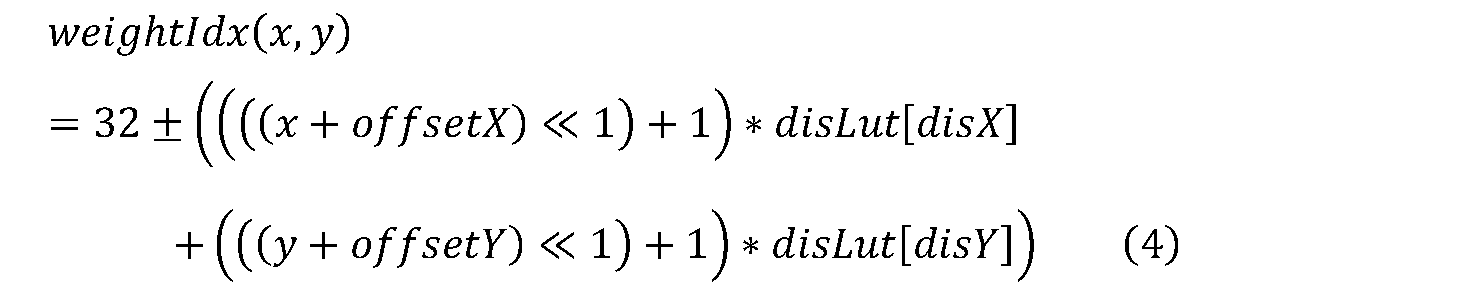
ECM(Enhanced Compression Model)として知られる探究ソフトウェアでは、VVCのGPMが新たな機能で拡張される。これらの機能のうちの1つが、同一ブロック内においてイントラ予測とインター予測とを混合することである。これら2つの予測は、図97に示したような複数の幾何学的分割モードのうちの1つに従って組み合わせられる。
DIMDの使用がビットストリームにおいてシグナリングされる場合、2つの角度イントラ予測モードが、再構成隣接サンプルの勾配値に基づいて導出される。そして、2つの角度イントラ予測モードが、勾配値から導出された重みを用いて、Planarイントラ予測モードと組み合わせられる。
VVCでは、例えば図31に示されるような正方形ブロックに対するイントラ予測モードとは異なる追加の角度イントラ予測モードが非正方形矩形ブロックに対して用いられ得る。具体的には、ブロックの幅と高さとの比に応じて選択される1つ以上の角度イントラ予測モードのそれぞれが、水平方向又は垂直方向に対して45°よりも大きい角度をなす予測方向を有する角度イントラ予測モードに置き換えられる。ここで、水平方向又は垂直方向は、具体的には、隣接参照画素列の法線方向に対応する。
非正方形矩形ブロックの場合、イントラインター混合予測における幾何学的分割モードとイントラ予測モードとのマッピングが修正される。


上記の例では、幾何学的分割モードの境界に平行な予測方向を有する狭角イントラ予測モードが決定される。しかしながら、幾何学的分割モードの境界に対して平行とは異なる関係を有する別の狭角イントラ予測モードが決定されてもよい。
上記に示された符号化装置100及び復号装置200の構成及び処理の代表例を以下に示す。
上述された各例における符号化装置100及び復号装置200は、それぞれ、画像符号化装置及び画像復号装置として利用されてもよいし、動画像符号化装置及び動画像復号装置として利用されてもよい。
以上の各実施の形態において、機能的又は作用的なブロックの各々は、通常、MPU(micro processing unit)及びメモリ等によって実現可能である。また、機能ブロックの各々による処理は、ROM等の記録媒体に記録されたソフトウェア(プログラム)を読み出して実行するプロセッサなどのプログラム実行部として実現されてもよい。当該ソフトウェアは、配布されてもよい。当該ソフトウェアは、半導体メモリなどの様々な記録媒体に記録されてもよい。なお、各機能ブロックをハードウェア(専用回路)によって実現することも可能である。
図106は、コンテンツ配信サービスを実現する適切なコンテンツ供給システムex100の全体構成を示す図である。通信サービスの提供エリアを所望の大きさに分割し、各セル内にそれぞれ、図示された例における固定無線局である基地局ex106、ex107、ex108、ex109、ex110が設置されている。
また、ストリーミングサーバex103は複数のサーバ又は複数のコンピュータであって、データを分散して処理したり記録したり配信するものであってもよい。例えば、ストリーミングサーバex103は、CDN(Contents Delivery Network)により実現され、世界中に分散された多数のエッジサーバとエッジサーバ間をつなぐネットワークによりコンテンツ配信が実現されていてもよい。CDNでは、クライアントに応じて物理的に近いエッジサーバが動的に割り当てられる。そして、当該エッジサーバにコンテンツがキャッシュ及び配信されることで遅延を減らすことができる。また、いくつかのタイプのエラーが発生した場合又はトラフィックの増加などにより通信状態が変わる場合に複数のエッジサーバで処理を分散したり、他のエッジサーバに配信主体を切り替えたり、障害が生じたネットワークの部分を迂回して配信を続けることができるので、高速かつ安定した配信が実現できる。
互いにほぼ同期した複数のカメラex113及び/又はスマートフォンex115などの端末により撮影された異なるシーン、又は、同一シーンを異なるアングルから撮影した画像或いは映像を統合して利用することが増えてきている。各端末で撮影した映像は、別途取得した端末間の相対的な位置関係、又は、映像に含まれる特徴点が一致する領域などに基づいて統合される。
図107は、コンピュータex111等におけるwebページの表示画面例を示す図である。図108は、スマートフォンex115等におけるwebページの表示画面例を示す図である。図107及び図108に示すようにwebページが、画像コンテンツへのリンクであるリンク画像を複数含む場合があり、閲覧するデバイスによってその見え方は異なる。画面上に複数のリンク画像が見える場合には、ユーザが明示的にリンク画像を選択するまで、又は画面の中央付近にリンク画像が近付く或いはリンク画像の全体が画面内に入るまで、表示装置(復号装置)は、リンク画像として各コンテンツが有する静止画又はIピクチャを表示してもよいし、複数の静止画又はIピクチャ等でgifアニメのような映像を表示してもよいし、ベースレイヤのみを受信し、映像を復号及び表示してもよい。
また、車の自動走行又は走行支援のため2次元又は3次元の地図情報などのような静止画又は映像データを送受信する場合、受信端末は、1以上のレイヤに属する画像データに加えて、メタ情報として天候又は工事の情報なども受信し、これらを対応付けて復号してもよい。なお、メタ情報は、レイヤに属してもよいし、単に画像データと多重化されてもよい。
また、コンテンツ供給システムex100では、映像配信業者による高画質で長時間のコンテンツのみならず、個人による低画質で短時間のコンテンツのユニキャスト、又はマルチキャスト配信が可能である。このような個人のコンテンツは今後も増加していくと考えられる。個人コンテンツをより優れたコンテンツにするために、サーバは、編集処理を行ってから符号化処理を行ってもよい。これは、例えば、以下のような構成を用いて実現できる。
また、これらの符号化又は復号処理は、一般的に各端末が有するLSIex500において処理される。LSI(large scale integration circuitry)ex500(図106参照)は、ワンチップであっても複数チップからなる構成であってもよい。なお、動画像符号化又は復号用のソフトウェアをコンピュータex111等で読み取り可能な何らかの記録メディア(CD-ROM、フレキシブルディスク、又はハードディスクなど)に組み込み、そのソフトウェアを用いて符号化又は復号処理を行ってもよい。さらに、スマートフォンex115がカメラ付きである場合には、そのカメラで取得した動画データを送信してもよい。このときの動画データはスマートフォンex115が有するLSIex500で符号化処理されたデータである。
図109は、図106に示されたスマートフォンex115のさらに詳細を示す図である。また、図110は、スマートフォンex115の構成例を示す図である。スマートフォンex115は、基地局ex110との間で電波を送受信するためのアンテナex450と、映像及び静止画を撮ることが可能なカメラ部ex465と、カメラ部ex465で撮像した映像、及びアンテナex450で受信した映像等が復号されたデータを表示する表示部ex458とを備える。スマートフォンex115は、さらに、タッチパネル等である操作部ex466と、音声又は音響を出力するためのスピーカ等である音声出力部ex457と、音声を入力するためのマイク等である音声入力部ex456と、撮影した映像或いは静止画、録音した音声、受信した映像或いは静止画、メール等の符号化されたデータ、又は、復号化されたデータを保存可能なメモリ部ex467と、ユーザを特定し、ネットワークをはじめ各種データへのアクセスの認証をするためのSIM(Subscriber Identity Module)ex468とのインタフェース部であるスロット部ex464とを備える。なお、メモリ部ex467の代わりに外付けメモリが用いられてもよい。
102 分割部
102a ブロック分割決定部
104 減算部
106 変換部
108 量子化部
108a 差分量子化パラメータ生成部
108b、204b 予測量子化パラメータ生成部
108c、204a 量子化パラメータ生成部
108d、204d 量子化パラメータ記憶部
108e 量子化処理部
110 エントロピー符号化部
110a 二値化部
110b、202b コンテキスト制御部
110c 二値算術符号化部
112、204 逆量子化部
114、206 逆変換部
116、208 加算部
118、210 ブロックメモリ
120、212 ループフィルタ部
120a、212a デブロッキング・フィルタ処理部
120b、212b SAO処理部
120c、212c ALF処理部
122、214 フレームメモリ
124、216 イントラ予測部
126、218 インター予測部
126a、a2、b2 メモリ
126b 補間画像導出部
126c 勾配画像導出部
126d オプティカルフロー導出部
126e 補正値導出部
126f 予測画像補正部
128、220 予測制御部
130、222 予測パラメータ生成部
200 復号装置
202 エントロピー復号部
202a 二値算術復号部
202c 多値化部
204e 逆量子化処理部
224 分割決定部
1201 境界判定部
1202、1204、1206 スイッチ
1203 フィルタ判定部
1205 フィルタ処理部
1207 フィルタ特性決定部
1208 処理判定部
a1、b1 プロセッサ
Claims (19)
- 映像のカレントブロックをビットストリームから復号する復号方法であって、
幾何学的分割モードに従って、前記カレントブロックにおける2つのパーティションを決定し、
複数の幾何学的分割モードと複数の角度イントラ予測モードとのマッピング関係を用いて、前記幾何学的分割モードから角度イントラ予測モードを導出し、
前記角度イントラ予測モードに従って、前記2つのパーティションのうちの第1パーティションを予測し、
前記角度イントラ予測モードの導出では、
前記カレントブロックの形状が正方形である場合、第1マッピング関係を前記マッピング関係として用いて、前記角度イントラ予測モードを導出し、
前記カレントブロックの形状が正方形でない場合、前記第1マッピング関係とは異なる第2マッピング関係を前記マッピング関係として用いて、前記角度イントラ予測モードを導出する、
復号方法。 - 前記第1マッピング関係は、前記幾何学的分割モードと第1狭角イントラ予測モードとのマッピング関係を含み、
前記第2マッピング関係は、前記幾何学的分割モードと第2狭角イントラ予測モードとのマッピング関係を含み、
前記第1狭角イントラ予測モードが前記複数の角度イントラ予測モードのサブセットに含まれる場合において、
(i)前記第1狭角イントラ予測モードの予測方向が水平方向又は垂直方向に対して斜め45°の方向である場合、前記第2狭角イントラ予測モードは、前記第1狭角イントラ予測モードの予測方向とは反対の予測方向を有し、
(ii)前記第1狭角イントラ予測モードの予測方向が水平方向又は垂直方向に対して斜め45°の方向でない場合、前記第2狭角イントラ予測モードは、前記第1狭角イントラ予測モードの第1インデックス値に固定オフセット値の加算又は減算を適用することで得られる第2インデックス値を有し、広角イントラ予測モードにリマッピングされ、
前記第1狭角イントラ予測モードが前記複数の角度イントラ予測モードのサブセットに含まれない場合において、前記第2狭角イントラ予測モードは、前記第1狭角イントラ予測モードと同じである、
請求項1に記載の復号方法。 - 前記固定オフセット値は1である、
請求項2に記載の復号方法。 - 前記複数の角度イントラ予測モードのサブセットは、前記カレントブロックの幅と高さとの違いによって定められる、
請求項2又は3に記載の復号方法。 - 前記第1狭角イントラ予測モードの予測方向は、前記2つのパーティションの間の境界に平行であり、
前記広角イントラ予測モードの予測方向は、前記境界に平行である、
請求項2又は3に記載の復号方法。 - 前記第1狭角イントラ予測モードの予測方向は、前記2つのパーティションの間の境界に対して一定角度を有し、
前記広角イントラ予測モードの予測方向は、前記境界に対して前記一定角度を有する、
請求項2又は3に記載の復号方法。 - 前記第1マッピング関係は、前記複数の幾何学的分割モードと、複数の狭角イントラ予測モードである前記複数の角度イントラ予測モードとのマッピング関係であり、
前記第2マッピング関係は、前記複数の幾何学的分割モードと、複数の狭角イントラ予測モード及び1つ以上の広角イントラ予測モードを含む前記複数の角度イントラ予測モードとのマッピング関係である、
請求項1に記載の復号方法。 - 前記第1パーティションの予測方法を示す第1予測モードインジケータ、及び、前記2つのパーティションのうちの第2パーティションの予測方法を示す第2予測モードインジケータを前記ビットストリームから復号し、
前記第1予測モードインジケータは、前記幾何学的分割モードから導出される前記角度イントラ予測モードが前記第1パーティションの予測に用いられることを前記第1パーティションの予測方法として示す、
請求項1~3及び7のいずれか1項に記載の復号方法。 - 映像のカレントブロックをビットストリームに符号化する符号化方法であって、
幾何学的分割モードに従って、前記カレントブロックにおける2つのパーティションを決定し、
複数の幾何学的分割モードと複数の角度イントラ予測モードとのマッピング関係を用いて、前記幾何学的分割モードから角度イントラ予測モードを導出し、
前記角度イントラ予測モードに従って、前記2つのパーティションのうちの第1パーティションを予測し、
前記角度イントラ予測モードの導出では、
前記カレントブロックの形状が正方形である場合、第1マッピング関係を前記マッピング関係として用いて、前記角度イントラ予測モードを導出し、
前記カレントブロックの形状が正方形でない場合、前記第1マッピング関係とは異なる第2マッピング関係を前記マッピング関係として用いて、前記角度イントラ予測モードを導出する、
符号化方法。 - 前記第1マッピング関係は、前記幾何学的分割モードと第1狭角イントラ予測モードとのマッピング関係を含み、
前記第2マッピング関係は、前記幾何学的分割モードと第2狭角イントラ予測モードとのマッピング関係を含み、
前記第1狭角イントラ予測モードが前記複数の角度イントラ予測モードのサブセットに含まれる場合において、
(i)前記第1狭角イントラ予測モードの予測方向が水平方向又は垂直方向に対して斜め45°の方向である場合、前記第2狭角イントラ予測モードは、前記第1狭角イントラ予測モードの予測方向とは反対の予測方向を有し、
(ii)前記第1狭角イントラ予測モードの予測方向が水平方向又は垂直方向に対して斜め45°の方向でない場合、前記第2狭角イントラ予測モードは、前記第1狭角イントラ予測モードの第1インデックス値に固定オフセット値の加算又は減算を適用することで得られる第2インデックス値を有し、広角イントラ予測モードにリマッピングされ、
前記第1狭角イントラ予測モードが前記複数の角度イントラ予測モードのサブセットに含まれない場合において、前記第2狭角イントラ予測モードは、前記第1狭角イントラ予測モードと同じである、
請求項9に記載の符号化方法。 - 前記固定オフセット値は1である、
請求項10に記載の符号化方法。 - 前記複数の角度イントラ予測モードのサブセットは、前記カレントブロックの幅と高さとの違いによって定められる、
請求項10又は11に記載の符号化方法。 - 前記第1狭角イントラ予測モードの予測方向は、前記2つのパーティションの間の境界に平行であり、
前記広角イントラ予測モードの予測方向は、前記境界に平行である、
請求項10又は11に記載の符号化方法。 - 前記第1狭角イントラ予測モードの予測方向は、前記2つのパーティションの間の境界に対して一定角度を有し、
前記広角イントラ予測モードの予測方向は、前記境界に対して前記一定角度を有する、
請求項10又は11に記載の符号化方法。 - 前記第1マッピング関係は、前記複数の幾何学的分割モードと、複数の狭角イントラ予測モードである前記複数の角度イントラ予測モードとのマッピング関係であり、
前記第2マッピング関係は、前記複数の幾何学的分割モードと、複数の狭角イントラ予測モード及び1つ以上の広角イントラ予測モードを含む前記複数の角度イントラ予測モードとのマッピング関係である、
請求項9に記載の符号化方法。 - 前記第1パーティションの予測方法を示す第1予測モードインジケータ、及び、前記2つのパーティションのうちの第2パーティションの予測方法を示す第2予測モードインジケータを前記ビットストリームに符号化し、
前記第1予測モードインジケータは、前記幾何学的分割モードから導出される前記角度イントラ予測モードが前記第1パーティションの予測に用いられることを前記第1パーティションの予測方法として示す、
請求項9~11及び15のいずれか1項に記載の符号化方法。 - コンピュータ用の非一時的なコンピュータ読み取り可能な記録媒体であって、
カレントブロックを復号する復号処理をコンピュータに行わせるビットストリームを記憶し、
前記復号処理では、
幾何学的分割モードに従って、前記カレントブロックにおける2つのパーティションを決定し、
複数の幾何学的分割モードと複数の角度イントラ予測モードとのマッピング関係を用いて、前記幾何学的分割モードから角度イントラ予測モードを導出し、
前記角度イントラ予測モードに従って、前記2つのパーティションのうちの第1パーティションを予測し、
前記角度イントラ予測モードの導出では、
前記カレントブロックの形状が正方形である場合、第1マッピング関係を前記マッピング関係として用いて、前記角度イントラ予測モードを導出し、
前記カレントブロックの形状が正方形でない場合、前記第1マッピング関係とは異なる第2マッピング関係を前記マッピング関係として用いて、前記角度イントラ予測モードを導出する、
非一時的なコンピュータ読み取り可能な記録媒体。 - 映像のカレントブロックをビットストリームから復号する復号装置であって、
回路と、
前記回路に接続されたメモリとを備え、
前記回路は、動作において、
幾何学的分割モードに従って、前記カレントブロックにおける2つのパーティションを決定し、
複数の幾何学的分割モードと複数の角度イントラ予測モードとのマッピング関係を用いて、前記幾何学的分割モードから角度イントラ予測モードを導出し、
前記角度イントラ予測モードに従って、前記2つのパーティションのうちの第1パーティションを予測し、
前記角度イントラ予測モードの導出では、
前記カレントブロックの形状が正方形である場合、第1マッピング関係を前記マッピング関係として用いて、前記角度イントラ予測モードを導出し、
前記カレントブロックの形状が正方形でない場合、前記第1マッピング関係とは異なる第2マッピング関係を前記マッピング関係として用いて、前記角度イントラ予測モードを導出する、
復号装置。 - 映像のカレントブロックをビットストリームに符号化する符号化装置であって、
回路と、
前記回路に接続されたメモリとを備え、
前記回路は、動作において、
幾何学的分割モードに従って、前記カレントブロックにおける2つのパーティションを決定し、
複数の幾何学的分割モードと複数の角度イントラ予測モードとのマッピング関係を用いて、前記幾何学的分割モードから角度イントラ予測モードを導出し、
前記角度イントラ予測モードに従って、前記2つのパーティションのうちの第1パーティションを予測し、
前記角度イントラ予測モードの導出では、
前記カレントブロックの形状が正方形である場合、第1マッピング関係を前記マッピング関係として用いて、前記角度イントラ予測モードを導出し、
前記カレントブロックの形状が正方形でない場合、前記第1マッピング関係とは異なる第2マッピング関係を前記マッピング関係として用いて、前記角度イントラ予測モードを導出する、
符号化装置。
Priority Applications (3)
| Application Number | Priority Date | Filing Date | Title |
|---|---|---|---|
| EP23788349.1A EP4510567A4 (en) | 2022-04-13 | 2023-04-12 | DECODING METHOD, ENCODING METHOD, DECODING DEVICE AND ENCODING DEVICE |
| CN202380030307.3A CN118923106A (zh) | 2022-04-13 | 2023-04-12 | 解码方法、编码方法、解码装置和编码装置 |
| US18/904,357 US20250030846A1 (en) | 2022-04-13 | 2024-10-02 | Decoding method, encoding method, decoder, and, encoder |
Applications Claiming Priority (2)
| Application Number | Priority Date | Filing Date | Title |
|---|---|---|---|
| EP22168179.4 | 2022-04-13 | ||
| EP22168179.4A EP4262204A1 (en) | 2022-04-13 | 2022-04-13 | Encoder, decoder, encoding method, and decoding method |
Related Child Applications (1)
| Application Number | Title | Priority Date | Filing Date |
|---|---|---|---|
| US18/904,357 Continuation US20250030846A1 (en) | 2022-04-13 | 2024-10-02 | Decoding method, encoding method, decoder, and, encoder |
Publications (1)
| Publication Number | Publication Date |
|---|---|
| WO2023199931A1 true WO2023199931A1 (ja) | 2023-10-19 |
Family
ID=81308412
Family Applications (1)
| Application Number | Title | Priority Date | Filing Date |
|---|---|---|---|
| PCT/JP2023/014813 Ceased WO2023199931A1 (ja) | 2022-04-13 | 2023-04-12 | 復号方法、符号化方法、復号装置及び符号化装置 |
Country Status (4)
| Country | Link |
|---|---|
| US (1) | US20250030846A1 (ja) |
| EP (2) | EP4262204A1 (ja) |
| CN (1) | CN118923106A (ja) |
| WO (1) | WO2023199931A1 (ja) |
Families Citing this family (4)
| Publication number | Priority date | Publication date | Assignee | Title |
|---|---|---|---|---|
| US12574507B2 (en) * | 2022-09-09 | 2026-03-10 | Qualcomm Incorporated | Intra prediction fusion with reduced complexity in video coding |
| WO2025157201A1 (en) * | 2024-01-26 | 2025-07-31 | Mediatek Inc. | Methods and apparatus of intra merge mode for template-based intra mode derivation |
| US20250324053A1 (en) * | 2024-04-12 | 2025-10-16 | Qualcomm Incorporated | Inter ciip and inter geo mode transform set selection for lfnst and nspt in video coding |
| WO2026001800A2 (zh) * | 2025-06-18 | 2026-01-02 | 深圳传音控股股份有限公司 | 处理方法、处理设备及存储介质 |
Citations (1)
| Publication number | Priority date | Publication date | Assignee | Title |
|---|---|---|---|---|
| WO2023015157A1 (en) * | 2021-08-02 | 2023-02-09 | Tencent America LLC | Constraint of intra mode for geometric partition mode with inter and intra prediction |
-
2022
- 2022-04-13 EP EP22168179.4A patent/EP4262204A1/en active Pending
-
2023
- 2023-04-12 EP EP23788349.1A patent/EP4510567A4/en active Pending
- 2023-04-12 CN CN202380030307.3A patent/CN118923106A/zh active Pending
- 2023-04-12 WO PCT/JP2023/014813 patent/WO2023199931A1/ja not_active Ceased
-
2024
- 2024-10-02 US US18/904,357 patent/US20250030846A1/en active Pending
Patent Citations (1)
| Publication number | Priority date | Publication date | Assignee | Title |
|---|---|---|---|---|
| WO2023015157A1 (en) * | 2021-08-02 | 2023-02-09 | Tencent America LLC | Constraint of intra mode for geometric partition mode with inter and intra prediction |
Non-Patent Citations (5)
| Title |
|---|
| "High Efficiency Video Coding", ISO/IEC 23008-2 HEVC |
| ABDOLI M. ET AL.: "Non-CE3: Decoder-side Intra Mode Derivation with Prediction Fusion Using Planar", JVET-00449, JVET (JOINT VIDEO EXPERTS TEAM) OF ITU-T SG 16 WP 3 AND ISO/IEC JTC 1/SC 29/WG11, 15TH MEETING, 3 July 2019 (2019-07-03) |
| CAO K. ET AL.: "EE2-related: Fusion for template-based intra mode derivation", JVET-W0123, JVET (JOINT VIDEO EXPERTS TEAM) OF ITU-T SG16 WP 3 AND ISO/IEC JTC 1/SC 29, 23TH MEETING, TELECONFERENCE, 2021 |
| See also references of EP4510567A4 |
| Y. KIDANI (KDDI), H. KATO (KDDI), K. KAWAMURA (KDDI), H. JANG (LGE), S. KIM, J. LIM (LGE), Z. DENG (BYTEDANCE), K. ZHANG, L. ZHANG: "EE2-3.1: GPM with inter and intra prediction (JVET-X0166)", 25. JVET MEETING; 20220112 - 20220121; TELECONFERENCE; (THE JOINT VIDEO EXPLORATION TEAM OF ISO/IEC JTC1/SC29/WG11 AND ITU-T SG.16 ), 4 January 2022 (2022-01-04), XP030300270 * |
Also Published As
| Publication number | Publication date |
|---|---|
| EP4510567A1 (en) | 2025-02-19 |
| CN118923106A (zh) | 2024-11-08 |
| EP4510567A4 (en) | 2025-07-16 |
| US20250030846A1 (en) | 2025-01-23 |
| EP4262204A1 (en) | 2023-10-18 |
Similar Documents
| Publication | Publication Date | Title |
|---|---|---|
| JP7389283B2 (ja) | 符号化装置及び復号装置 | |
| JP7785050B2 (ja) | 符号化装置、復号装置、符号化方法及び復号方法 | |
| JP7738485B2 (ja) | 符号化装置、復号装置、符号化方法、および復号方法 | |
| JP7772982B2 (ja) | ビットストリームの送信装置、およびビットストリームの送信方法 | |
| JP7781322B2 (ja) | ビットストリーム送信装置 | |
| JP7776678B2 (ja) | 符号化装置、復号装置、符号化方法、および復号方法 | |
| CN114521331A (zh) | 编码装置、解码装置、编码方法和解码方法 | |
| JP2023174956A (ja) | 復号装置及び符号化装置 | |
| CN118923106A (zh) | 解码方法、编码方法、解码装置和编码装置 | |
| JP2025137635A (ja) | 符号化装置、復号装置、符号化方法及び復号方法 | |
| JP2026041929A (ja) | ビットストリームの送信装置及び送信方法並びに非一時的記憶媒体 | |
| JP2026009212A (ja) | 符号化装置、復号装置、符号化方法及び復号方法 | |
| JP2025137605A (ja) | 符号化装置、復号装置及びビットストリーム生成装置 | |
| WO2023199783A1 (ja) | 復号方法、符号化方法、復号装置及び符号化装置 | |
| CN115606186B (zh) | 编码装置、解码装置、编码方法以及解码方法 | |
| JP7453970B2 (ja) | 復号装置 | |
| KR20230011298A (ko) | 부호화 장치, 복호 장치, 부호화 방법, 및 복호 방법 | |
| JP2024023810A (ja) | 符号化装置 | |
| WO2024009967A1 (ja) | 復号装置、符号化装置、復号方法、および符号化方法 | |
| WO2025239155A1 (ja) | 符号化装置、復号装置、ビットストリーム生成装置、符号化方法、復号方法及びビットストリーム生成方法 | |
| JP2025123281A (ja) | 符号化装置、復号装置、符号化方法及び復号方法 | |
| WO2023013736A1 (ja) | 符号化装置、復号装置、符号化方法、および復号方法 | |
| WO2021187603A1 (ja) | 符号化装置、復号装置、画像処理装置、符号化方法、復号方法、画像処理方法、ビットストリーム送信装置、および、非一時的記憶媒体 |
Legal Events
| Date | Code | Title | Description |
|---|---|---|---|
| 121 | Ep: the epo has been informed by wipo that ep was designated in this application |
Ref document number: 23788349 Country of ref document: EP Kind code of ref document: A1 |
|
| WWE | Wipo information: entry into national phase |
Ref document number: 202380030307.3 Country of ref document: CN |
|
| WWE | Wipo information: entry into national phase |
Ref document number: 2023788349 Country of ref document: EP |
|
| NENP | Non-entry into the national phase |
Ref country code: DE |
|
| ENP | Entry into the national phase |
Ref document number: 2023788349 Country of ref document: EP Effective date: 20241113 |