WO2024157776A1 - データ処理装置、データ処理方法、及びプログラム - Google Patents
データ処理装置、データ処理方法、及びプログラム Download PDFInfo
- Publication number
- WO2024157776A1 WO2024157776A1 PCT/JP2024/000399 JP2024000399W WO2024157776A1 WO 2024157776 A1 WO2024157776 A1 WO 2024157776A1 JP 2024000399 W JP2024000399 W JP 2024000399W WO 2024157776 A1 WO2024157776 A1 WO 2024157776A1
- Authority
- WO
- WIPO (PCT)
- Prior art keywords
- data
- virtual
- mapping
- column
- data structure
- Prior art date
- Legal status (The legal status is an assumption and is not a legal conclusion. Google has not performed a legal analysis and makes no representation as to the accuracy of the status listed.)
- Ceased
Links
Images







Classifications
-
- G—PHYSICS
- G06—COMPUTING OR CALCULATING; COUNTING
- G06F—ELECTRIC DIGITAL DATA PROCESSING
- G06F16/00—Information retrieval; Database structures therefor; File system structures therefor
- G06F16/20—Information retrieval; Database structures therefor; File system structures therefor of structured data, e.g. relational data
- G06F16/22—Indexing; Data structures therefor; Storage structures
-
- G—PHYSICS
- G06—COMPUTING OR CALCULATING; COUNTING
- G06F—ELECTRIC DIGITAL DATA PROCESSING
- G06F16/00—Information retrieval; Database structures therefor; File system structures therefor
- G06F16/20—Information retrieval; Database structures therefor; File system structures therefor of structured data, e.g. relational data
- G06F16/21—Design, administration or maintenance of databases
- G06F16/211—Schema design and management
-
- G—PHYSICS
- G06—COMPUTING OR CALCULATING; COUNTING
- G06F—ELECTRIC DIGITAL DATA PROCESSING
- G06F16/00—Information retrieval; Database structures therefor; File system structures therefor
- G06F16/20—Information retrieval; Database structures therefor; File system structures therefor of structured data, e.g. relational data
- G06F16/22—Indexing; Data structures therefor; Storage structures
- G06F16/221—Column-oriented storage; Management thereof
-
- G—PHYSICS
- G06—COMPUTING OR CALCULATING; COUNTING
- G06F—ELECTRIC DIGITAL DATA PROCESSING
- G06F16/00—Information retrieval; Database structures therefor; File system structures therefor
- G06F16/20—Information retrieval; Database structures therefor; File system structures therefor of structured data, e.g. relational data
- G06F16/22—Indexing; Data structures therefor; Storage structures
- G06F16/2228—Indexing structures
-
- G—PHYSICS
- G06—COMPUTING OR CALCULATING; COUNTING
- G06F—ELECTRIC DIGITAL DATA PROCESSING
- G06F16/00—Information retrieval; Database structures therefor; File system structures therefor
- G06F16/20—Information retrieval; Database structures therefor; File system structures therefor of structured data, e.g. relational data
- G06F16/22—Indexing; Data structures therefor; Storage structures
- G06F16/2228—Indexing structures
- G06F16/2272—Management thereof
-
- G—PHYSICS
- G06—COMPUTING OR CALCULATING; COUNTING
- G06F—ELECTRIC DIGITAL DATA PROCESSING
- G06F16/00—Information retrieval; Database structures therefor; File system structures therefor
- G06F16/20—Information retrieval; Database structures therefor; File system structures therefor of structured data, e.g. relational data
- G06F16/22—Indexing; Data structures therefor; Storage structures
- G06F16/2282—Tablespace storage structures; Management thereof
-
- G—PHYSICS
- G06—COMPUTING OR CALCULATING; COUNTING
- G06F—ELECTRIC DIGITAL DATA PROCESSING
- G06F16/00—Information retrieval; Database structures therefor; File system structures therefor
- G06F16/20—Information retrieval; Database structures therefor; File system structures therefor of structured data, e.g. relational data
- G06F16/24—Querying
- G06F16/245—Query processing
- G06F16/2455—Query execution
-
- G—PHYSICS
- G06—COMPUTING OR CALCULATING; COUNTING
- G06F—ELECTRIC DIGITAL DATA PROCESSING
- G06F16/00—Information retrieval; Database structures therefor; File system structures therefor
- G06F16/20—Information retrieval; Database structures therefor; File system structures therefor of structured data, e.g. relational data
- G06F16/24—Querying
- G06F16/248—Presentation of query results
-
- G—PHYSICS
- G06—COMPUTING OR CALCULATING; COUNTING
- G06F—ELECTRIC DIGITAL DATA PROCESSING
- G06F16/00—Information retrieval; Database structures therefor; File system structures therefor
- G06F16/20—Information retrieval; Database structures therefor; File system structures therefor of structured data, e.g. relational data
- G06F16/25—Integrating or interfacing systems involving database management systems
- G06F16/258—Data format conversion from or to a database
-
- G—PHYSICS
- G06—COMPUTING OR CALCULATING; COUNTING
- G06F—ELECTRIC DIGITAL DATA PROCESSING
- G06F16/00—Information retrieval; Database structures therefor; File system structures therefor
- G06F16/20—Information retrieval; Database structures therefor; File system structures therefor of structured data, e.g. relational data
- G06F16/28—Databases characterised by their database models, e.g. relational or object models
Definitions
- This disclosure relates to a data processing device, a data processing method, and a program.
- This disclosure has been made in consideration of the above points, and provides technology that allows indexes that enable sorting, searching, and aggregation of real table-format data to be inherited by virtual table-format data.
- a data processing device has a data manipulation unit that performs a sort operation, a search operation, or an aggregation operation on virtual tabular data composed of virtual columns having a second data structure obtained by converting a first data structure of one or more columns included in one or more tabular data by a predetermined mapping, using the second data structure as an index.
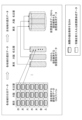
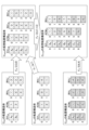
- FIG. 1 is a diagram for explaining an example of virtual table-format data hierarchically constructed starting from D5A that holds values.
- FIG. FIG. 13 is a diagram for explaining an example (part 1) of mapping A.
- FIG. 13 is a diagram for explaining an example (part 2) of mapping A.
- FIG. 13 is a diagram for explaining an example of allocation.
- FIG. 13 is a diagram for explaining an example of an allocation method using enumeration mapping.
- FIG. 13 is a diagram for explaining an example of an allocation method using linear function mapping.
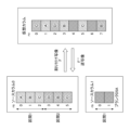
- FIG. 2 illustrates an example of a source column and a virtual column.
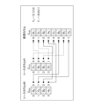
- FIG. 2 is a diagram showing an example of a source column, a transposed structure, and a virtual transposed structure;
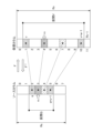
- FIG. 13 is a diagram for explaining an example of layout mapping of two-level virtual table-format data.
- FIG. 13 is a diagram illustrating an example of a virtual transposed structure of two-level virtual tabular data.
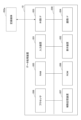
- 1 is a diagram illustrating an example of the overall configuration of a system including a data processing device according to an embodiment of the present invention.
- FIG. 1 is a diagram illustrating an example of a hardware configuration of a data processing device according to an embodiment of the present invention.
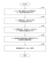
- 13 is a flowchart showing an example of the flow of a process for creating virtual tabular data.
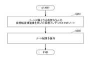
- 13 is a flowchart showing an example of the flow of a sort process on virtual table-format data.
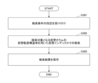
- 13 is a flowchart showing an example of the flow of a search process in virtual table-format data.
- 13 is a flowchart showing an example of the flow of a counting process for virtual table-format data.
- D5A data called tabular data
- D5A data called tabular data
- a method for creating new virtual tabular data from D5A or other virtual tabular data and a method for inheriting indexes of (real) tabular data to sort, search, and aggregate the virtual tabular data will be described. It will also be described how indexes can be inherited even when the virtual tabular data is constructed hierarchically.
- a data processing device 10 that can create such virtual tabular data and sort, search, and aggregate it will be described.
- Archive data such as IoT (Internet of Things) data, various observation data, and log data is being accumulated daily.
- IoT Internet of Things
- tabular data is compiled into one at regular intervals, such as daily or monthly, and added to the archive.
- Tabular data added to the archive can be considered read-only.
- Tabular data in such archives can be huge, and is often distributed over LANs (Local Area Networks) and the Internet.
- the first step is to generate new tabular data.
- New tabular data is created by UNIONing or JOINing multiple pieces of tabular data, or by extracting only the necessary columns. This can take a long time if the original tabular data is huge or distributed over a wide area network such as the Internet. Also, if the new tabular data is large, a large memory area is required to store it.
- the second step involves sorting, searching, and aggregating.
- the newly created tabular data is not indexed, so sorting, searching, and aggregating takes time.
- the sorting results when the new tabular data is large, the search results when the number of hits is large, and the aggregation results when they are large all require a large amount of storage space.
- the tabular data to be operated on may be, for example, one trillion records or 100,000 columns. Furthermore, combinations such as UNIONS and JOINS of the tabular data to be operated on may be stacked hierarchically. Furthermore, the tabular data to be operated on may be distributed on a LAN, or may be distributed on multiple HTTP (Hypertext Transfer Protocol) servers on the Internet.
- HTTP Hypertext Transfer Protocol
- a network system for mapping archive data can be constructed using D5A, a file format for tabular data with indexes on all columns that speed up sorting, searching, and aggregation; virtual tabular data that inherits values directly or indirectly from the D5A file; and virtual indexes on the virtual tabular data that use a data structure that is automatically established by directly or indirectly inheriting the data structure used by the D5A file index.
- the virtual tabular data and virtual indexes are immediately available for use simply by connecting them directly or indirectly to D5A, and they consume only a small amount of storage space.
- sorting results, search results, and aggregation results obtained using virtual indexes require only a small amount of storage space, no matter how large they are.
- This kind of network of mapping of archive data using D5A makes it possible for users to create virtual tabular data for each purpose and use the archive data distributed on the network interactively in a new way of using archive data. For example, it makes it possible for each organization to use archive data distributed to each department within the organization for various purposes, and on the Internet it makes it possible to combine and extract archive data such as IoT data from all over the world and use it in a variety of linked ways.
- D5A is a file format for table format data in which all columns have indexes that speed up sorting, searching, and aggregation.
- virtual table format data is table format data that inherits values from a D5A file (a file in D5A format) or other virtual table format data.
- the table format data from which it is inherited is called source table format data.
- a column on D5A is called a D5A column, and an index that speeds up sorting, searching, and aggregation of a D5A column is called a D5A index.
- virtual table format data is called a virtual column and virtual index.
- source table format data is called a source column and source index.
- the data structure used by a D5A index is called a transposed structure
- the data structure used by a virtual index is called a virtual transposed structure
- the data structure used by a source index is called a source transposed structure.
- virtual table format data may be called “mapped table format data” or the like, and similarly, virtual columns may be called “mapped columns” or the like.
- the first step is a step of generating new tabular data by performing UNION or JOIN or extracting only the necessary columns
- the second step is a step of sorting, searching, and aggregating.
- the reason why the first step takes time is because it takes time to read, compare, and store the values. Therefore, instead, an approach can be considered in which there is tabular data that will be the source tabular data, and a mapping defined by a correspondence table and rules that defines which cells in the source tabular data are mapped to which cells in the newly created tabular data is used to create new tabular data using that mapping.
- a mapping defined by a correspondence table and rules that defines which cells in the source tabular data are mapped to which cells in the newly created tabular data is used to create new tabular data using that mapping.
- the new tabular data does not need to have values, which is an advantage especially when the new tabular data is huge.
- the new tabular data can be displayed in just the short time it takes to load the mapping definition, and only a small amount of memory is required to hold the mapping definition. This new tabular data does not hold values, but inherits values from the original tabular data, so it is virtual tabular data.
- the problem in the first step can be solved with such virtual tab
- the second step takes time because there are no indexes on the columns of the newly created tabular data, and because it takes time to write out the sort results, search results, and aggregation results, which are often huge.
- the time-consuming problem is solved by the fact that every column of the virtual tabular data above automatically has a virtual index that speeds up the sorting, searching, and aggregation of that column, and because this virtual index can hold even huge sort results, search results, and aggregation results with only a small amount of memory space, thereby reducing the write time.
- the virtual index only uses a small amount of memory space to store these results, the storage space problem is also solved. In this way, the problem in the second step can be solved by virtual indexes.
- the D5A file which is expressed in a storage format for tabular data called D5A, holds the values that form the basis of this virtual tabular data and the data structure that forms the basis of the data structure used by the virtual index.
- ⁇ D5A Storage format of tabular data that serves as a source of values and indexes>
- Virtual tabular data inherits values from one or more source tabular data.
- the source tabular data is either another virtual tabular data or tabular data called a D5A file.
- the virtual tabular data inherits values from yet another source tabular data, and finally arrives at a D5A file. Therefore, it can be said that the virtual tabular data is hierarchically structured, directly or indirectly inheriting values from the D5A file.
- the virtual index uses a virtual transposed structure to speed up sorting, searching, and aggregation.
- the virtual transposed structure is established automatically by inheriting one or more source transposed structures.
- a source transposed structure is either a virtual transposed structure on another virtual tabular data, or a transposed structure on a D5A file.
- the virtual transposed structure inherits yet another source transposed structure, and finally arrives at a transposed structure on a D5A file. Therefore, it can be said that the virtual transposed structure is established hierarchically by directly or indirectly inheriting the transposed structure on a D5A file.
- D5A is a storage format for tabular data that provides values to virtual tabular data and provides transpose structures to virtual transpose structures, with a D5A index that holds values and uses transpose structures for all its columns.
- FIG. 1 shows a process for combining meteorological observation data from Sunday to Saturday for each region of Tokyo, Osaka, and Nagoya. This process is performed in two stages, first combining seven daily data for each region into weekly data, and then juxtaposing the weekly data into one table format data.
- 21 daily data for one week for three regions on the left side of FIG. 1 are stored in a 55A file.
- the three table format data for each region in the center of FIG. 1 are virtual table format data.
- Each of these virtual table format data uses the seven D5A files for one week on the left side of FIG. 1 as source table format data, extracts necessary columns from them, and then performs a UNION.
- One virtual table format data on the right side of FIG. 1 juxtaposes the three virtual table format data for each region in the center of FIG. 1 as source table format data.
- the mapping network for archive data starts with the D5A file, with virtual tabular data built hierarchically on top of it.
- virtual tabular data is automatically equipped with virtual indexes, allowing any column to be sorted, searched, and aggregated in a short time, and only a small amount of memory is required to store the sort results, search results, and aggregation results.
- This type of virtual tabular data can be created and used by users themselves, and it is expected to promote widespread use of archive data.
- mapping> D5A virtual tabular data, and virtual indexes are all described as a combination of mappings from a continuous interval of natural numbers starting from 0 to some value (also often a natural number).
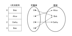
- This mapping can be expressed as a one-dimensional array (Array) with subscripts (indexes) starting from 0, so it is called A-mapping.
- Array one-dimensional array
- indexes indexes
- A-maps can be created by combining A-maps in various ways.
- A-map S which represents the result string of a search
- A-map C- A which represents column A
- A-map C- B which represents column B
- A-map representing the search results of column B can be obtained.
- S can be any A-map that represents a result string
- C -A and C- B can be any A-map that represents columns. They can exist on a local storage device or on a network.
- Such a combination of A-maps can be said to be an algebraic combination.
- a virtual A mapping is an A mapping that uses one or more A mappings as the combining source, has a known overall size, and allows for the extraction of any i-th part from the combining source. Since a virtual A mapping is also an A mapping, it is possible to combine virtual A mappings to create further virtual A mappings hierarchically.
- a column of virtual tabular data is a type of virtual A mapping, and can be created hierarchically.
- An index is a mechanism that is realized by a data structure for indexing and an algorithm that uses that data structure.
- a virtual index is an index that uses one or more virtual A mappings as the data structure for indexing, and can be created hierarchically.
- the second advantage of the A-map is that it can be decomposed to create a new A-map.
- decomposing the A-map it is possible to create and use a new A-map with functions that were not present in the A-map before decomposition.
- One particularly effective decomposition is the LP decomposition (decomposition into A-map L and A-map P) of the A-map M that defines the correspondence (mapping) between cells in tabular data.
- Decomposing M into L and P makes it possible to search for elements efficiently using a bisection search in L, and to find the inverse mapping in P.
- M can be any A-map that defines the mapping, and L automatically becomes an A-map that allows for a bisection search, and P automatically becomes an A-map with an inverse. Since the decomposition of the A-map produces a new A-map, it can be said to be an algebraic decomposition.
- D5A a storage format for tabular data in which every column has an index that allows for high-speed sorting, searching, and aggregation.
- D5A and the A mapping it is possible to define virtual tabular data.
- This virtual tabular data is automatically provided with a virtual index that uses one or more A mappings as the data structure for the index. This makes it possible to realize a network system of archive data mappings that allows archive data distributed across the network to be used in various combinations.
- mapping can be expressed as a one-dimensional array, but when discussing its mapping aspect it is called a mapping, and when discussing its operations it is called an array. Accordingly, when treated as a mapping it will be called a domain and value range, and when it is an array containing columns or tabular data it will be called a record number and value. However, the notation for the A mapping will be as much as possible as an array.
- Notation 2 When specifying the domain n of A mapping A, write it as A (n) . According to this notation, a column is written as, for example, C (R) where R is the total number of records.
- a (n) [i] The i-th element of the A-map A (n) is written as A (n) [i]. Therefore, A (n) ⁇ (A (n) [0], A (n) [1], ..., A (n) [n-1]).
- index operator that combines A-maps>
- a (n) ⁇ B (m) (n) (A (n) [B (m) (n) [0]], ..., A (n) [B (m) (n) [m- 1]])
- Formula (1) The above index operator has the following properties 1 to 3.
- Property 2 The size of the array that represents the combination result is the size of the array on the right.
- Property 3 The data type of the array representing the join result is the data type of the left array.
- the number of types of values that can appear in the A mapping obtained as a result of combining A mappings with the index operator is equal to or less than the size of the smallest A mapping among the A mappings combined with the index operator. This is an index similar to the rank in a matrix.
- unique decomposition methods are of special value, as they make it possible to speed up sorting and searching, and to find inverse mappings.
- unique decomposition methods SN decomposition, LP decomposition, and spectral decomposition.
- SN decomposition This is a method of decomposing one A mapping into two, and there is only one way in which the left A mapping of the two resulting A mappings holds only the values that appear in the left A mapping, and holds these values uniquely and in ascending order. This decomposition is called SN decomposition.
- the first item on the right-hand side which is unique and ascending, is called the SVL (Sorted Value List).
- SVL (Alice, Bob, Cathy).
- C (R) SVL (K) ⁇ NNC (R) (K) ; i, j ⁇ 0,...,K-1 and i ⁇ j ⁇ SVL (K) [i] ⁇ SVL (K) [j] Equation (2)
- the upper part indicates that column C (R) is decomposed into SVL (K) and NNC (R) (K)
- the lower part indicates that the elements of SVL (K) are arranged in ascending order.
- NNC (R) (K) is an A-map of size R whose elements are natural numbers 0, ..., K-1, as can be seen from the notation.
- Step 1-1 Add the position in the A mapping to each value of (Bob, Alice, Cathy, Bob) to create ((Bob, 0), (Alice, 1), (Cathy, 2), (Bob, 3)).
- Step 1-2 Sort the values and positions while evaluating their relative magnitude to obtain ((Alice, 1), (Bob, 0), (Bob, 3), (Cathy, 2)).
- LP decomposition When LP decomposition is performed, it is possible to use L to determine the presence or absence of elements in M and their order, and to use P to find the inverse. Note that LP decomposition can be performed using the same algorithm as SN decomposition.
- Spectral decomposition The above notation 7 expresses the position (index) on the A map where each value appears as a new A map. This is called the spectral decomposition of the A map. Spectral decomposition makes it possible to view the A map from the range to the domain, enabling various algorithms. Below is an example showing how spectral decomposition of a column, which is an A map, makes it easy to sort, search, and aggregate the column.
- the sorting is performed by removing values from the spectral decomposition of the column Alice: (1) + Bob: (0, 3) + Cathy: (2) to obtain (1) + (0, 3) + (2), and performing the concatenation defined in Notation 5 to obtain the sorted result string (1, 0, 3, 2).
- Search result C (R)
- R is the total number of records
- ⁇ is a key value
- w is the number of transposed record numbers belonging to the key value ⁇
- X is an array of transposed record numbers.
- Step 2-1 Add the position in the A mapping to each value of (Bob, Alice, Cathy, Bob) to create ((Bob, 0), (Alice, 1), (Cathy, 2), (Bob, 3)).
- Step 2-2 Sort the values and positions while evaluating their relative magnitude to obtain ((Alice, 1), (Bob, 0), (Bob, 3), (Cathy, 2)).
- Step 2-3 Grouping the positions in the A map with the same values completes the spectral decomposition Alice: (1) + Bob: (0, 3) + Cathy: (2).
- A-maps can be classified according to four criteria: associativity, searchability, whether they represent a set, and whether their inverse can be easily found. Keeping these classifications in mind will help you understand the following explanations, so we will explain them here.
- A-maps with natural numbers as elements can be placed on both sides of an index operator.
- A-maps without natural numbers can only be placed on the left side of an index operator.
- An A-map whose elements are arranged in ascending order can be used to efficiently search for whether a particular element exists and, if so, where it is located, using a bisection search. Such an A-map is called an ascending array.
- An A-map whose elements are unique and ascending order can be searched for a certain value, and if a match exists, it will be the only one. Such an A-map is called a unique ascending array.
- Symmetric arrays form a group with respect to the index operator. Therefore, there exists an identity and an inverse.
- the inverse of P is used to identify cells in the source tabular data from cells in the virtual tabular data.
- an index is established when the size W of the sort/search/aggregation results of the target column is known, and when i ⁇ 0, 1, ..., W-1 is specified, the i-th row of the sort/search/aggregation results can be read in approximately O(log(R)) or less time.
- CSV Common Separated Values
- D5A is a collection of D5A columns, which are columns of D5A with the same structure. Each D5A column is a juxtaposition of the two structures described below.
- the first structure is for obtaining column values, and is the part enclosed by the dashed line in Figure 4.
- This structure can be configured to either (a) store the column, which is the A mapping, as is, (b) store the SVL and NNC obtained by SN decomposition of the column, or (c) store both.
- (a) storing as is the performance of reading values improves, but algorithms using NNC cannot be used.
- (b) storing SVL and NNC algorithms using NNC can be used, but the performance of reading values decreases.
- the size of the D5A file increases. In this embodiment, the case of (b) will be explained.
- the second structure is for the D5A index, and is the part enclosed by the dashed line in Figure 4.
- This structure consists of SVL, ACM, and INV, and is called the transposed structure.
- the transposed structure is the spectral decomposition of the D5A column described above rewritten in the form of an A mapping. The details of the transposed structure will be described later.
- a transposed structure i.e., the second structure
- it will be combined with the first structure above to form a D5A column, and collecting the D5A columns will result in D5A.
- the structure for obtaining the column values can be created by SN decomposition of column C (R) .
- the following information 1 to 4 can also be obtained from the SVL.
- the number of different values in a column, K can be determined from SVL (K) . For example, in the example shown in FIG.
- a bisection search of SVL can tell you whether a value v exists in a column. Also, if the value v exists, you can tell what number value v is.
- SVL is the aggregation dimension. Note that previously, sorting was required to create an aggregation dimension.
- transposed structure is a structure for the D5A index.
- spectral decomposition of a column allows for high-speed sorting, searching, and aggregation, but there are two difficult points to handle with spectral decomposition. The first is that it is not made of A mapping, so it cannot be accessed using an index operator (first problem).
- first problem when trying to obtain the i-th item in the sorted result column, it is necessary to search for the i-th item while adding w 0 , w 1 , ... (second problem).
- the transposed structure is the result of converting the spectral decomposition into three A mappings, which solves these two points. Below, we will explain its definition and how to create it.
- transposition structure Definition of transposition structure and method of creating it from spectral decomposition
- the definition of the transposition structure is shown below.
- SVL (K) is the A-map obtained by simply arranging the value parts of the spectral decomposition in equation (3), ⁇ 0 , ⁇ 1 , ..., ⁇ K -1 . It is also the same as SVL (K) obtained by equation (4).
- Step 3-2 ACM (K) (R+1) is
- INV is a record number corresponding to ⁇ 0 ⁇ 1 ⁇ . . . ⁇ K ⁇ 1
- INV is an array of transposed record numbers.
- the transposed structure is ⁇ (Alice, Bob, Cathy): (1, 3, 4), (1, 0, 3, 2)>.
- Spectral decomposition is not an A-map, and requires an addition operation of w i to obtain the i-th element of the sorted result sequence.
- the transposed structure derived from spectral decomposition is a structure consisting of three A-maps, which can solve the first problem, and since the i-th element of the sorted result sequence can be obtained with INV[i], the second problem can also be solved.
- the spectral decomposition can be obtained from the transposed structure in D5A in the following manner.
- ⁇ i SVL (K) [i]. Also, if we predetermine that ACM[ ⁇ 1] ⁇ 0, then
- the i-th term of the spectral decomposition can be obtained as follows.
- the first term of the spectral decomposition is given by:
- the following information 5 to information 8 can also be obtained.
- the i-th record number in the sorted result can be read as follows:
- i-th record number of sorted result INV[i] Formula (9)
- the record numbers with the ith smallest value can be read out as the following array.
- Equation (10) Let i0 be the smallest i0 that satisfies v0 ⁇ SVL[ i0 ], and let i1 be the largest i1 that satisfies SVL[ i1 ] ⁇ i1 , (INV (R) (R) [ACM (K) [ i0-1 ]], ...,INV (R) (R) [ACM (K) [ i1 ]-1]) Equation (10) For example, in the example shown in FIG.
- An index can be created with a transposed structure
- the requirement for an index to be valid is that the size W of the sorted, searched, and tabulated results is known, and when i ⁇ 0, 1, ..., W-1 is specified, the i-th row of the sorted, searched, and tabulated results can be read in approximately O(log(R)) or less.
- search The case of formula (10) will now be described.
- the size of the search result is found to be ACM (K) [ i1 ]-ACM (K )[ i0-1 ].
- the i-th element of the search result can be read in O(1) using (INV (R) (R) [ACM (K) [ i0-1 ]], ...,INV (R) (R) [ACM (K) [ i1 ]-1])[i].
- ICV (R) (R) [ACM (K) [ i0-1 ]] ...,INV (R) (R) [ACM (K) [ i1 ]-1]
- i] (0, 3, 2)[i].
- the inverted structure meets the requirements for creating an index for searching.
- the size of the aggregation result is known to be K from information 1 above.
- the i-th value of the aggregation result is given by information 2 above, and can be obtained in O(1).
- the number of occurrences of the i-th value of the aggregation result is given by equation (8), and can be obtained in O(1). Therefore, the transposed structure meets the requirements for creating an index on aggregation.
- the above makes it possible to create a D5A index that uses a transposed structure to speed up sorting, searching, and aggregation.
- sort results The results of sorting, searching, and aggregation using the D5A index require only a small amount of storage space (sort results).
- the sorted results are already stored in INV, and no new storage area is required.
- search results The case of formula (10) will be described.
- the search results are given as an array (INV (R) (R) [ACM (K) [ i0-1 ]], ..., INV (R) (R) [ACM (K) [ i1 ]-1]).
- INV and ACM have already been created, and the memory area required to hold the search results is only the storage area for i0 and i1 , regardless of the number of hits.
- the i-th value of the counted result is given by the above information 2, and does not require any new storage area.
- the number of occurrences of the i-th value of the counted result is given by equation (8), and does not require any new storage area.
- D5A has the role of supplying values to virtual table data and indexes to virtual indexes.
- SVL and NNC obtained by SN decomposition of a column
- information 1 to information 4 listed above.
- a D5A index can be created using a transposed structure (in other words, a transposed structure can be used as a data structure for indexes in sorting, searching, and aggregation).
- a D5A index not only speeds up sorting, searching, and aggregation, but can also hold the results of sorting, searching, and aggregation in only a small amount of memory space.
- ⁇ Virtual tabular data> For example, when performing a JOIN or UNION in an RDB (Relational Database), the source tabular data is read, compared, the data to be written is created, the storage location is determined, and the data is written to a newly secured storage area. This requires time and storage space. This is the first step in trying to utilize archived tabular data. The larger the newly generated tabular data is, the more serious this problem becomes. This is because it takes a long time to generate and requires a large storage area. Moreover, often only a small portion of the generated tabular data is used.
- RDB Relational Database
- Virtual tabular data solves the above problem by creating the necessary parts when they are needed.
- the cell in the source tabular data that corresponds to that cell is referenced at that time and displayed.
- a mapping that defines the correspondence between the cells in the virtual tabular data and the cells in one or more source tabular data must be defined in advance. This mapping can be from virtual tabular data to multiple source tabular data, or conversely, from multiple source tabular data to virtual tabular data; both are essentially the same.
- the destination of the mapping in the former is a set of two pieces of information, namely, which cell in which source tabular data
- the latter requires only one piece of information, namely, which cell in the virtual tabular data, and is therefore easier to define. Therefore, the latter will be explained below. Both require an inverse mapping.
- the virtual index requires an inverse mapping, and in the latter, it is necessary when the virtual tabular data references the source tabular data to obtain a value.
- an allocation mapping The latter mapping of which cells in each source tabular data correspond to which cells in the virtual tabular data is called an allocation mapping.
- an actual allocation mapping defines a mapping from each source column, which is a column in the source tabular data, to a virtual column, which is a column in the virtual tabular data.
- Each source column is divided into one or more intervals, and for each interval, cells in that interval are associated with cells in the virtual column using a correspondence table or rules. This correspondence for each interval is called an interval mapping.
- An allocation mapping is the sum of all interval mappings.
- rs indicates the record number on the source table format data
- rv indicates the record number on the virtual table format data.
- a virtual column which is a column on virtual table format data, is composed of allocation mappings from one or more source columns.
- the virtual column is allocated from source column 0 and source column 1.
- the blank D5A with source column 1 in the bottom left of Figure 5 is a D5A that is automatically generated programmatically when a virtual column is generated.
- Blank D5A supplies blank values to unassigned cells in the virtual column, so that the virtual column satisfies the bijection condition described below. If the bijection condition is satisfied, a virtual index is automatically provided for the virtual table format data.
- it is not necessary to sort, search, or aggregate virtual table format data For example, there are cases when you want to use the entire result of a UNION or JOIN as is. In that case, you can of course define and use virtual table format data without considering the bijection condition.
- Each source column is divided into one or more source intervals.
- source column 0 is divided into interval 1 and interval 2.
- There are two types of mappings from each source interval to a virtual column i.e., interval mappings).
- the first is an enumeration mapping defined by an A-mapping M whose elements are natural numbers and have no duplicates.
- the second is a linear function mapping defined by a linear function.
- the former enumeration mapping can define any allocation mapping, but it consumes a lot of memory space.
- the latter linear function mapping is a mapping in which the M of the enumeration mapping is replaced by a linear function. It consumes only a small amount of memory space and can define even large interval mappings, but it can only handle allocations with regularity.
- interval mappings have been defined for all source intervals, the allocation mapping is complete.
- any of the above interval mappings are defined, their inverse mappings and the conditions for the existence of the inverse mappings are also determined.
- the source interval in which the above inverse mappings exist is identified from the record number of the virtual column, then the inverse mapping of that interval mapping is used to identify the record number in the source column, and the value is obtained from that record number and displayed.
- ⁇ Interval mapping by enumeration mapping and its inverse mapping> 6 shows an example of allocation by enumeration mapping.
- Rs is the size of the source column
- rs is the record number of the source column
- Rv is the size of the virtual column
- rv is the record number of the virtual column
- Q is an interval on the source column
- q is the start position of interval Q
- u is the length of interval Q
- V is an interval on the virtual column corresponding to interval Q
- v is the start position of interval V
- w is the length of interval V.
- M is an A-map whose elements are natural numbers with no duplicates, and can be subjected to LP decomposition.
- the top line of equation (12) shows the LP decomposition.
- L is a unique ascending-order array, and a bisection search can be used to determine whether an element exists and, if so, where it appears.
- Equation (12) shows how to find the position in L where rv appears, and j is its position. If j cannot be found, it means that rv has not accepted the mapping from source section Q, and there is no inverse mapping.
- Rs represents the size of the source column
- rs represents the record number of the source column
- Rv represents the size of the virtual column
- rv represents the record number of the virtual column
- Q represents an interval on the source column
- q represents the start position of interval Q
- u represents the length of interval Q
- V represents an interval on the virtual column corresponding to interval Q
- v represents the start position of interval V
- w represents the length of interval V.
- rs (rv-b)/a Formula (14)
- v ⁇ rv ⁇ v+w is not true
- rs is not an integer
- rv is not the range of F.
- Equation (13) that defines the linear function mapping.
- Fig. 7 the numbers written beside the source column and virtual column are record numbers.
- Source interval 1 of source column 0 is interval mapped by linear function type mapping
- source interval 2 of source column 0 is interval mapped by enumeration type mapping
- source interval 1 of source column 1 is interval mapped by linear function type mapping.
- the definition of each interval mapping is as follows.
- the virtual tabular data is composed of the following information.
- Step 4-2 If L 0 [i] ⁇ L 1 [j], set i ⁇ i+1 and return to step 4-1. However, if the result of setting i ⁇ i+1 is that i exceeds the maximum value of the index representing the elements of L 0 , it is determined that there is no collision and the process ends.
- Step 4-3 If L 0 [i]>L 1 [j], set j ⁇ j+1 and return to step 4-1. However, if the result of setting j ⁇ j+1 is that j exceeds the maximum value of the index representing the elements of L 1 , it is determined that there is no collision and the process ends.
- a 0 and a 1 are integers of 1 or more
- b 0 and b 1 are integers.
- Step 5-2 If y0 ⁇ y1 , set x0 ⁇ x0 + MaxInt(1, ( y1 - y0 ) div a0 ) and return to step 5-1. However, if the result of setting x0 ⁇ x0 + MaxInt(1, ( y1 - y0 ) div a0 ) is x0 > MinInt( N0 - 1, LCM( a0 , a1 ) div a0 ), it is determined that there is no collision and the process ends.
- Step 5-3 If y0 > y1 , set x1 ⁇ - x1 + MaxInt(1, ( y0 - y1 ) div a1 ) and return to step 5-1. However, if the result of setting x1 ⁇ - x1 + MaxInt(1, ( y0 - y1 ) div a1 ) is x1 > MinInt( N1 - 1, LCM( a0 , a1 ) div a1 ), it is determined that there is no collision and the process ends.
- MaxInt is a function that selects the maximum integer
- MinInt is a function that selects the minimum integer
- div is an integer division function (the remainder is truncated)
- LCM is a function that returns the least common multiple.
- (v 1 , . . . , v 1 +w 1 -1) is an ascending array of size M.
- Step 6-3 If y 0 (n) ⁇ y 1 (m), return to step 6-1 with n ⁇ (y 1 (m)-y 0 (n)) diva 0. However, if n ⁇ N as a result of setting n ⁇ (y 1 (m)-y 0 (n)) diva 0 , end the process as "no collision".
- ⁇ Virtual Index> So far, we have explained a method for creating virtual tabular data that directly or indirectly inherits values from D5A. Below, we will explain why a virtual transposed structure is automatically established on virtual tabular data by directly or indirectly inheriting the transposed structure on D5A.
- a virtual index that uses it as a data structure for indexing is also automatically established.
- a virtual index has the same functions and characteristics as a D5A index because it uses the same algorithm as a D5A index, but only uses a virtual transposed structure instead of a transposed structure. In other words, it is possible to speed up sorting, searching, and aggregation of columns, and even huge sorting results, search results, and aggregation results can be held in only a small memory area.
- the virtual transposed structure is a structure that has a virtual SVL, virtual ACM, and virtual INV.
- the virtual SVL, virtual ACM, and virtual INV are virtual arrays.
- a virtual array is a mechanism with the same functionality as an array, in that it does not hold values like virtual tabular data, its size W is known in advance, and when i ⁇ 0,1,...,W-1 is specified, the i-th element can be extracted in approximately O(log(R)) or less.
- the virtual SVL, virtual ACM, and virtual INV are automatically established if the allocation mapping that defines the virtual tabular data satisfies the following bijective conditions.
- the source column is bijective If the source column is D5A, it can be said that the source column is bijective. If the source column is a virtual column, it can be said that the source column is bijective if it satisfies 1 to 3 above.
- a virtual transposed structure can be constructed from multiple transposed structures, and then verify that a virtual index that uses this virtual transposed structure can perform sorting, searching, and aggregation at high speed, and that sort results, search results, and aggregation results can be stored by simply allocating a small amount of new memory space.
- a virtual index that uses this virtual transposed structure can perform sorting, searching, and aggregation at high speed, and that sort results, search results, and aggregation results can be stored by simply allocating a small amount of new memory space.
- further virtual transposed structures can be created hierarchically from virtual transposed structures and transposed structures, and that a virtual index that uses this can also perform sorting, searching, and aggregation at high speed, and that sort results, search results, and aggregation results can be stored by simply allocating a small amount of new memory space.
- we verify that the operation of a hierarchically created virtual transposed structure can be easily understood by using spectral decomposition.
- FIG. 8 shows a virtual column C V (8) defined from source column #0: C 0 (4) and source column #1: C 1 (4) .
- the transposed structure of source column #0, the transposed structure of source column #1, and the virtual transposed structure are shown in Fig. 9.
- SVL, ACM, and INV in the transposed structure of source column #0 are denoted as SVL0 , ACM0 , and INV0 , respectively
- SVL, ACM, and INV in the transposed structure of source column #1 are denoted as SVL1 , ACM1 , and INV1 , respectively.
- SVL, ACM, and INV in the virtual transposed structure of the virtual column are denoted as SVLV , ACMV , and INVV , respectively.
- INV 0 and INV 1 are arrays that store transposed record numbers, and since the record numbers in the source column are mapped to the record numbers in the virtual column by allocation mapping, when reading INV 0 and INV 1 , they must be converted to INV 0 ' and INV 1 ', respectively.
- INV 0 ' and INV 1 ' can be calculated by the following formula (15).
- Formula (15)-2 A method for constructing a virtual transposed structure will be described below in the order of virtual arrays SVL V , ACM V , and INV V , using FIG. 9 as an example.
- v is selected from SVL 0 or SVL 1.
- this v follows the above rule that determines the magnitude relationship taking into account the order of the source column.
- the sum j of the number of values smaller than v in SVL 0 and SVL 1 is found. If j ⁇ i, v' larger than v is selected and the above is repeated. The same process is carried out when j>i (but v' smaller than v is selected).
- the above method of finding SVL V [i] can be done in approximately O(log(K)). Since the size of SVL V is known and the i-th element can be extracted in O(log(R)) or less, it can be considered that a virtual array SVL V exists.
- a virtual array SVL V (A 0 , B 0 , B 1 , C 0 , C 1 , D 1 ) can be created.
- ACM V size of ACM V is obtained as the size of SVL V.
- ACM V [i] can be done in approximately O(log(K)). Then, since the size of ACM V is known and the i-th element can be extracted in O(log(R)) or less, it can be considered that a virtual array ACM V exists.
- a virtual array ACM V (1, 3, 5, 6, 7, 8) can be created.
- the size of INV V is known to be R, where R is the sum of the sizes of the source columns.
- j is the number of the interval on INV V that ACM V determines.
- ACM V The size of ACM V is defined as K V.
- K V is the sum of the sizes of ACM 0 and ACM 1.
- an appropriate j is selected from 0, 1, ..., K V -1, and the interval ACM V [j-1] to ACM V [j]-1 is obtained using the method explained in "Method of constructing virtual array ACM V ".
- the above method of finding INV V [i] can be performed in approximately O(log(K)). Since the size of INV V is known and the i-th element can be extracted efficiently, it can be considered that a virtual array INV V exists.
- Sorting with a Virtual Index Let's try sorting with a virtual index using a virtual inverted structure. Since NNC is not shown in Figures 8 and 9, we use C v (8) in Figure 8 instead. The sorting result is as follows.
- a inverted structure is a data structure for a D5A index, and for similar reasons, we can say that a virtual inverted structure is a data structure for a virtual index.
- the virtual transposed structure is composed of references to the transposed structure of the source column, but if the source column is a virtual column, the transposed structure is also a virtual transposed structure, so in that case, the virtual transposed structure is constructed hierarchically.
- FIG. 10 shows an example in which virtual tabular data C V0 (5) is created using D5A files C 0 (3) and C 1 (2) , and further virtual tabular data C V1 (8 ) is created using the virtual tabular data C V0 (5) and D5A file C 2 (3) .
- the definition of the allocation mapping is shown below.
- Sorting using a virtual index of hierarchically created virtual table format data Let's try sorting using a virtual index that uses a hierarchically created virtual inverted structure. Since NNC is not shown in Figures 10 and 11, we will use CV1(8) in Figure 10 instead. The sorting result is as follows.
- C V0(5) A 0 : (3) + B 0 : (2,0)
- C 1 (2) A 1 : (4) + C 1 (1) Therefore, C V0(5) can be expressed as follows:
- C V0 (5) and C 2 (3) can be expressed by spectral decomposition as follows.
- C V0 (5) A 0 :(1)+A 1 :(5)+B 0 :(7,2)+C 1 (3)
- C 2 (3) A 2 : (4) + B 2 : (6) + D 2 : (0) Therefore, C V1(8) can be expressed as follows:
- the search result string for "C" is (7, 2, 6, 3). The calculation can be done in the same way as in Table 3 above. Therefore, when doing manual calculations, calculations using spectral decomposition are easy to understand and excellent. It can be seen that...
- Fig. 12 An example of the overall configuration of a system including a data processing device 10 according to this embodiment is shown in Fig. 12.
- the data processing device 10 according to this embodiment is communicably connected to database servers that are distributed and arranged on a network 20 such as the Internet.
- These database servers store at least one of D5A and virtual table format data.
- the data processing device 10 has a virtual tabular data creation unit 101, a sorting unit 102, a search unit 103, a compilation unit 104, and a memory unit 105.
- the virtual tabular data creation unit 101, the sorting unit 102, the search unit 103, and the compilation unit 104 are realized, for example, by a process in which one or more programs installed in the data processing device 10 are executed by a processor such as a CPU (Central Processing Unit).
- the memory unit 105 is realized, for example, by a HDD (Hard Disk Drive), SSD (Solid State Drive), flash memory, etc.
- the virtual tabular data creation unit 101 creates virtual tabular data having information 1 to 5 described in the above "Virtual tabular data configuration method.” In addition, when defining the interval mapping 5 described in the above “Virtual tabular data configuration method,” the virtual tabular data creation unit 101 determines whether or not there is a collision in the allocation destinations due to the interval mapping (allocation mapping) by the method described in "Detecting collisions of allocations from different intervals.”
- the sort unit 102 executes sorting with a virtual index using the virtual transposed structure of the virtual table-format data described above. For example, the sort unit 102 uses the virtual column to be sorted of the virtual table-format data and the virtual INV included in the virtual transposed structure of the virtual column, and calculates the sort result by index calculation of those.
- the search unit 103 When the search unit 103 receives search conditions, it executes a search with a virtual index using the virtual transposed structure of the virtual table-format data described above. For example, the search unit 103 calculates formulas (8) and (10) using the virtual column to be searched in the virtual table-format data, the search conditions for that virtual column, and the virtual INV and virtual ACM included in the virtual transposed structure of that virtual column, and then calculates the search results by index calculation of the virtual column and the calculation results of formulas (8) and (10).
- the aggregation unit 104 performs aggregation using a virtual index that uses the virtual transposed structure of the virtual table-format data described above. For example, the aggregation unit 104 performs aggregation using the above information 2 and formula (8) using the virtual transposed structure of the virtual column to be aggregated of the virtual table-format data.
- the storage unit 105 stores various data (e.g., virtual table format data, D5A, sorting results, search results, aggregation results, etc.).
- data e.g., virtual table format data, D5A, sorting results, search results, aggregation results, etc.
- FIG. 13 An example of the hardware configuration of the data processing device 10 according to this embodiment is shown in Fig. 13. As shown in Fig. 13, the data processing device 10 according to this embodiment has an input device 201, a display device 202, an external I/F 203, a communication I/F 204, a RAM (Random Access Memory) 205, a ROM (Read Only Memory) 206, an auxiliary storage device 207, and a processor 208. Each of these pieces of hardware is connected to each other via a bus 209 so as to be able to communicate with each other.
- a bus 209 so as to be able to communicate with each other.
- the input device 201 is, for example, a keyboard, a mouse, a touch panel, a physical button, etc.
- the display device 202 is, for example, a display, a display panel, etc. Note that the data processing device 10 does not have to have at least one of the input device 201 and the display device 202, for example.
- the external I/F 203 is an interface with external devices such as a recording medium 203a.
- recording media 203a include a CD (Compact Disc), a DVD (Digital Versatile Disk), an SD memory card (Secure Digital memory card), and a USB (Universal Serial Bus) memory card.
- the communication I/F 204 is an interface for connecting the data processing device 10 to the network 20.
- the RAM 205 is a volatile semiconductor memory (storage device) that temporarily stores programs and data.
- the ROM 206 is a non-volatile semiconductor memory (storage device) that can store programs and data even when the power is turned off.
- the auxiliary storage device 207 is a non-volatile storage device such as an HDD, SSD, or flash memory.
- the processor 208 is, for example, a CPU or other type of arithmetic device.
- the hardware configuration shown in FIG. 13 is an example, and the data processing device 10 may have other hardware configurations.
- the data processing device 10 may have multiple auxiliary storage devices 207 or multiple processors 208, may not have some of the hardware shown in the figure, or may have various hardware other than the hardware shown in the figure.
- Step S101 First, the virtual table-format data creation unit 101 accepts the number of records of the virtual table-format data and the name and data type of the virtual column (information 1 and 2 described in "Virtual table-format data configuration method" above). Note that the number of records of the virtual table-format data and the name and data type of the virtual column are specified, for example, by the user.
- Step S102 Next, the virtual tabular data creation unit 101 accepts the specification of the URL or path of one or more source tabular data (the information of 3 described in the "Virtual tabular data configuration method" above).
- the URL or path of the one or more source tabular data is specified, for example, by the user. Also, the URL or path of one or more columns included in the one or more source tabular data may be specified.
- Step S103 Next, the virtual tabular data creation unit 101 accepts the definition of the source column and source section in each source tabular data (information 4 described in "Virtual tabular data configuration method" above). Note that the definition of the source column and source section in each source tabular data is specified by, for example, the user.
- Step S104 Next, the virtual tabular data creation unit 101 accepts the definition of the interval mapping for each source interval (the information in 5 described in the above "Virtual tabular data construction method") and calculates the definition of the inverse mapping. Note that the definition of the interval mapping and its inverse mapping for each source interval is specified, for example, by the user. Also, once the interval mapping is defined, its inverse mapping is automatically determined by equations (12) and (14) and stored in the storage unit 105.
- Step S105 Finally, the virtual tabular data creation unit 101 stores the information received in steps S101 to S104 above in the storage unit 105 as virtual tabular data.
- Step S201 The sort unit 102 executes a sort using a virtual index that uses the virtual transposed structure of the virtual column to be sorted among the virtual columns of the virtual table format data.
- Step S202 Then, the sorting unit 102 stores the sorting result in step S201 in the storage unit 105. However, the sorting unit 102 does not have to store the sorting result.
- Step S301 First, the search unit 103 accepts search conditions.
- Step S302 Next, the search unit 103 executes a search in a virtual index using the virtual transposed structure of the virtual column to be searched among the virtual columns of the virtual table format data.
- Step S303 The search unit 103 then stores the search results from step S302 in the storage unit 105.
- Step S401 The aggregation unit 104 performs aggregation using a virtual index that uses the virtual transposed structure of the virtual column to be aggregated, among the virtual columns of the virtual table format data.
- Step S402 The aggregation unit 104 then stores the aggregation result from step S303 in the storage unit 105. However, the aggregation unit 104 does not have to store the aggregation result.
- new virtual tabular data can be defined by allocation mapping using D5A or already defined virtual tabular data as source tabular data. Moreover, this virtual tabular data can be sorted, searched, and tallied at high speed using virtual indexes.
- An index is realized by a data structure for indexing and a set of algorithms that use that data structure to speed up processing.
- a transposed structure can be considered as a data structure for indexing that speeds up sorting, searching, and aggregation.
- a virtual transposed structure for a column can be created by rearranging the elements of the column from the transposed structure.
- a virtual transposed structure can also be created from multiple transposed structures.
- multiple virtual transposed structures can be hierarchically organized to create a further virtual transposed structure. In this way, a virtual transposed structure can be created hierarchically or by rearranging the elements of a column.
- An index algorithm that uses a transposed structure can also be applied to a virtual transposed structure, which becomes a virtual index. Existing indexes do not have a data structure for indexing that can be combined or hierarchically combined like a transposed structure, so inheritance is not possible when combining or hierarchically.
- REFERENCE SIGNS LIST 10 Data processing device 20 Network 101 Virtual table format data creation unit 102 Sorting unit 103 Search unit 104 Counting unit 105 Storage unit 201 Input device 202 Display device 203 External I/F 203a Recording medium 204 Communication I/F 205 RAM 206 ROM 207 Auxiliary storage device 208 Processor 209 Bus
Landscapes
- Engineering & Computer Science (AREA)
- Theoretical Computer Science (AREA)
- Databases & Information Systems (AREA)
- Data Mining & Analysis (AREA)
- Physics & Mathematics (AREA)
- General Engineering & Computer Science (AREA)
- General Physics & Mathematics (AREA)
- Software Systems (AREA)
- Computational Linguistics (AREA)
- Information Retrieval, Db Structures And Fs Structures Therefor (AREA)
Abstract
Description
IoT(Internet of Things)データ、様々な観測データ、ログデータ等のアーカイブデータの蓄積が日々進行している。これらの多くでは表形式データが日次や月次のように一定期間毎に1つにまとめられてアーカイブに追加されていくことが多い。アーカイブに追加された表形式データはReadOnlyと考えてよい。このようなアーカイブの表形式データは巨大になることがあるし、しばしばLAN(Local Area Network)上及びインターネット上に分散している。
上述したように、アーカイブの表形式データを活用しようとすると、一般に、第1ステップと第2ステップの2つのステップを必要とし、いずれのステップでも長い時間が掛かり、また大きい記憶領域を消費することが多い、という問題がある。なお、第1ステップはUNIONしたりJOINしたり必要なカラムのみを抽出したりして新たな表形式データを生成するステップ、第2ステップはソートしたり検索したり集計したりするステップである。
仮想表形式データは、1つ以上のソース表形式データから値を継承する。ソース表形式データは、別の仮想表形式データ、又は、D5Aファイルと呼ばれる表形式データ、のいずれかである。前者の場合、その仮想表形式データは更に別のソース表形式データから値を継承し最終的にD5Aファイルに辿り着く。したがって、仮想表形式データは直接的又は間接的にD5Aファイルから値を継承して階層的に成り立っているといえる。
アーカイブデータの写像のネットワークシステムの簡単な想定例を示し、ここまでに説明したD5A、仮想表形式データ、仮想インデックスの使用方法について、図1を参照しながら説明する。図1は、東京、大阪、名古屋の各地域の日曜日から土曜日の気象観測データを1つにまとめる処理を示している。この処理は2段階で行われ、まず地域毎に7つの日次データをまとめて週次データにし、次にそれらの週次データを並置して1つの表形式データにまとめている。ここで、図1の左側にある3地域1週間分の21個の日次データは55Aファイルに収容されている。図1の中央にある地域毎の3つの表形式データは仮想表形式データである。これらの仮想表形式データはそれぞれ図1の左側にある1週間分の7つのD5Aファイルをソース表形式データとして、それらから必要なカラムを抽出した上でUNIONしている。図1の右側にある1つの仮想表形式データは、図1の中央にある地域毎の3つの仮想表形式データをソース表形式データとして、それらを並置している。
D5A、仮想表形式データや仮想インデックスはすべて0から始まる自然数の連続区間から何等かの値(これも多くの場合は自然数)への写像の組み合わせで記述される。この写像は添字(インデックス)が0から始まる1次元配列(Array)で表せるので、これをA写像と呼ぶ。A写像を用いると対応関係を全体から眺めることが可能になり、その結果、集合や群としての性質を利用したアルゴリズムを導くことが可能になる。以下にA写像の利点を説明する。
インデックスが0から始まり、サイズNの1次元配列を考える。その1次元配列は定義域が0~N-1の自然数の連続区間、値域が最大N種類の離散区間である写像と見ることができる。これをA写像と呼ぶ。レコードに0から始まる連続するレコード番号が振られていれば、表形式データのカラムもレコード番号を定義域としたA写像とみなすことができる。
以下に一般的な配列の表記法を取り入れたA写像の表記を記載する。
A写像の結合を行って新たなA写像を作り出すインデックス演算子(Index Operator)と呼ぶ演算子・を以下で定義する。
上記のインデックス演算子には、以下の性質1~性質3に示す性質がある。
インデックス演算子を用いてA写像を結合すると、ただ1つのA写像が得られる。一方で、1つのA写像は様々なA写像に分解できる。例えば、(Bob,Alice,Cathy,Bob)は、(Bob,Alice,Cathy,Bob)=(Alice,Bob,Cathy)・(1,0,2,1)と分解することもできるし、(Bob,Alice,Cathy,Bob)=(Bob,Alice,Cathy)・(0,1,2,0)と分解することもできる。
1つのA写像を2つに分解する方法で、得られる2つのA写像のうちの左側のA写像が左辺のA写像に出現する値だけを保持し、それらの値をユニークかつ昇順に保持する場合は1通りしか存在しない。この分解をSN分解と呼ぶ。
i,j∈0,・・・,K-1かつi<j⇒SVL(K)[i]<SVL(K)[j]
式(2)
式(2)では上段でカラムC(R)がSVL(K)とNNC(R) (K)に分解されることを表しており、下段でSVL(K)の要素は昇順に並ぶことを表している。なお、NNC(R) (K)については、その表記から0,・・・,K-1の自然数を要素とするサイズRのA写像であることがわかる。
ここで、(Bob,Alice,Cathy,Bob)を例にSN分解のアルゴリズムの一例を述べる。SN分解のアルゴリズムでは、以下の手順1-1~手順1-5が実行される。
LP分解は、重複のない自然数を要素とするA写像M(Mapping projection)を2つに分解するSN分解の特殊なケースである。例えば、(5,2,7,3)=(2,3,5,7)・(2,0,3,1)はLP分解の例である。
上記の表記法7は各値にその値が出現するA写像上の位置(インデックス)を新たなA写像として表記するものである。これをA写像のスペクトル分解と呼ぶ。スペクトル分解により、A写像を値域から定義域に向かって見ることが可能になり、様々なアルゴリズムを可能にする。以下、A写像であるカラムのスペクトル分解によりカラムのソート・検索・集計が簡単にできるようになる例を示す。
図3に示す例で、ソートは、カラムのスペクトル分解Alice:(1)+Bob:(0,3)+Cathy:(2)から値を外して(1)+(0,3)+(2)とし、表記法5で定めた連結を行ってソート結果列(1,0,3,2)を得ることができる。なお、ソート結果はカラムC(R)=(Bob,Alice,Cathy,Bob)とソート結果列とを以下のように結合して得ることができる。
図3に示す例で、Bobの検索は、カラムのスペクトル分解Alice:(1)+Bob:(0,3)+Cathy:(2)からバイセクションサーチでBobのパートを特定し、それを取り出してBob:(0,3)を得て、検索結果列(0,3)を得ることができる。なお、検索結果は、カラムC(R)=(Bob,Alice,Cathy,Bob)と検索結果列とを以下のように結合して得ることができる。
図3に示す例で、集計は、カラムのスペクトル分解Alice:(1)+Bob:(0,3)+Cathy:(2)から値とその出現回数を取り出し、集計結果=Alice:1回、Bob:2回、Cathy:1回を得ることができる。
ここで、スペクトル分解を一般的に書き直すと以下となる。

w0=1,w1=2,w2=1
X0(1) (4)=(1),X1(2) (4)=(0,3),X2(1) (4)=(2)
(スペクトル分解のアルゴリズム)
ここで、(Bob,Alice,Cathy,Bob)を例にA写像をスペクトル分解するアルゴリズムの一例を示しておく。そのアルゴリズムは、以下の手順2-1~手順2-3からなる。
A写像は、結合性、検索性、集合を表しているかどうか、簡単に逆元が求まるか、という4つの指標で分類することができる。これらの分類を踏まえておくことは、これ以降の説明の理解に役立つため、ここで述べておく。
自然数を要素とするA写像はインデックス演算子の両側におくことができる。そうでないA写像はインデックス演算子の左側にしかおくことができない。
要素が昇順に並ぶA写像はバイセクションサーチを用いて特定の要素があるかどうか、ある場合はどこにあるかを効率的に検索することができる。このようなA写像を昇順配列と呼ぶ。要素がユニークかつ昇順であるA写像はある値で検索してマッチするものが存在する場合、それがただ一つになる。このようなA写像をユニーク昇順配列と呼ぶ。
A写像の要素に重複がなければそれは集合を表していると見なすことができる。ただし、本明細書では要素が自然数であることも前提に加える。本明細書では、集合は結果列であり自然数(レコード番号)を要素とするA写像であるためである。
自然数を要素とするA写像でそのサイズをNとするとき、そのA写像に0~N-1の値を持つ要素がすべて含まれる場合、インデックス演算子に関する逆元を簡単に求めることができる。これを対称配列と呼ぶ。対称配列Pの定義を以下に示す。
対称配列はインデックス演算子に関して群を作る。したがって、単位元と逆元が存在する。Pの逆元は仮想表形式データのセルからソース表形式データのセルを特定する際に使用される。
逆元:P[i]=j⇒P-1[j]=i
<D5A>
Rは表形式データのレコード数、Kはカラムの中に含まれる値の種類を指すものとする。このとき、表形式データとは、上から順に0~R-1の番号で識別されるR個のレコードと、左から順に番号又は名前で識別される1~複数のカラムとを持ち、1つのレコードと1つのカラムとで1つの値が定まり、カラム毎にそのカラムで保持されるデータのデータ型(例えば、整数、浮動小数点、文字列等)が1つに定まっているものをいう。また、インデックスが成立しているとは、対象カラムのソート・検索・集計結果のサイズWがわかり、i∈0,1,・・・,W-1を指定するとおよそO(log(R))以下の時間でソート・検索・集計結果のi行目を読み出せる状態になっていることをいう。
図4を参照しながらD5Aの内部構造を説明する。図4は、カラムC(4)=(Bob,Alice,Cathy,Bob)が含まれるCSV(Comma Separated Values)形式の表形式データとそのD5Aフォーマットを示している。
カラムの値を取得するための構造は、カラムC(R)をSN分解して作成することができる。例えば、図4に示す例の場合、C(4)=(Bob,Alice,Cathy,Bob)=(Alice,Bob,Cathy)・(1,0,2,1)となる。したがって、SVL(3)=(Alice,Bob,Cathy)、NNC(4) (3)=(1,0,2,1)となる。
したがって、カラムのi行目は以下の式で得られる。
例えば、図4に示す例の場合、カラムの1行目は(Alice,Bob,Cathy)・(1,0,2,1)[1]=Aliceとなる。
次に、D5Aインデックスのための構造である転置構造体の作成方法について説明する。カラムをスペクトル分解するとソート・検索・集計を高速に行えることを述べたが、スペクトル分解には2つの扱いにくい点がある。1つ目は、A写像でできていないため、インデックス演算子を用いてアクセスすることができない点(第1の問題点)である。2つ目は、ソート結果列のi番目を取得しようとすると、w0,w1,・・・を加算しながらi番目を探す必要がある点(第2の問題点)である。スペクトル分解を3つのA写像に変換したものが転置構造体であり、この2点を解決する。以下、その定義と作成方法を説明する。
転置構造体の定義を以下に示す。

手順3-1:SVL(K)は、式(3)のスペクトル分解の値部分であるλ0,λ1,・・・,λK-1をそのまま並べてA写像にしたものである。また、式(4)で得られるSVL(K)と同じである。



以下の方法でD5A内の転置構造体からスペクトル分解を得ることができる。


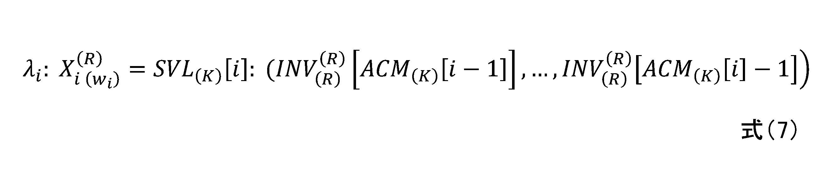

転置構造体を使うと、SVLから得られる情報(上記の情報1~情報4)に加えて、以下の情報5~情報8も得られる。
例えば、図4に示す例の場合、小さい方から1番目の値の出現回数は、ACM(K)[1]-ACM(K)[0]=3-1=2となる。
例えば、図4に示す例の場合、ソート結果の1番目のレコード番号は、INV[1]=0(Bob)として読み出せる。
例えば、図4に示す例の場合、小さい方から1番目の値(Bob)を持つレコード番号は、(INV[1],・・・,INV[2])=(0,3)として読み出せる。
例えば、図4に示す例の場合、値Bob~Cathyを持つレコード番号はi0=1、i1=2であるため、(INV[ACM[1-1]],・・・,INV[ACM[2]-1])=(INV[1],・・・,INV[4-1])=(0,3,2)として読み出せる。
上述したように、インデックスの成立要件は、ソート・検索・集計結果のサイズWがわかり、i∈0,1,・・・,W-1を指定するとおよそO(log(R))以下でソート・検索・集計結果のi行目を読み出せることである。以下、転置構造体でインデックスを作成できることを確かめる。
ソート結果のサイズはRであることがわかる。ソート結果のi番目の要素は式(9)を使いO(1)で読み出せる。したがって、転置構造体はソートについてインデックスを作成するための要件を満たす。
式(10)の場合について説明する。検索結果のサイズはACM(K)[i1]-ACM(K)[i0-1]であるとわかる。例えば、図4に示す例の場合、値Bob~Cathyを持つレコード番号はi0=1、i1=2であるため、ACM(K)[2]-ACM(K)[1-1]=4-1=3であるとわかる。
集計結果のサイズは上記の情報1からKであることがわかる。集計結果のi番目の値は上記の情報2で与えられ、O(1)で得られる。集計結果のi番目の値の出現回数は式(8)で与えられ、O(1)で得られる。したがって、転置構造体は集計についてインデックスを作成するための要件を満たす。
(ソート結果)
ソート結果は既にINVに保持されており、新たな記憶領域を必要としない。
式(10)の場合について説明する。検索結果は配列(INV(R) (R)[ACM(K)[i0-1]],・・・,INV(R) (R)[ACM(K)[i1]-1])で与えられている。そのうち、INV、ACMは既に作成されており、検索結果を保持するために必要とする記憶領域はヒット件数とは無関係にi0,i1の格納領域だけである。
集計結果のi番目の値は上記の情報2で与えられ、新たな記憶領域を必要としない。集計結果のi番目の値の出現回数は式(8)で与えられ、新たな記憶領域を必要としない。
例えば、RDB(Relational Database)でJOINやUNIONを行うとソース表形式データを読み出し、それらを比較し、書き出すデータを作り、その格納位置を決め、新たに確保した記憶領域上に書き出す。すると、時間と記憶領域とを必要とする。それがアーカイブの表形式データを活用しようとする際の第1ステップの問題である。この問題は、新たに生成される表形式データが巨大であればあるほど深刻になる。その生成に長い時間が掛かり、大きい記憶領域を必要とするためである。しかも、往々にして使用されるのは生成された表形式データのわずかな部分である。
図5を参照しながら割り付け写像の作成手順を説明する。なお、以下、rsはソース表形式データ上のレコード番号、rvは仮想表形式データ上のレコード番号を指すものとする。
図6は列挙型写像による割り付けの例を示している。図6において、Rsはソースカラムのサイズ、rsはソースカラムのレコード番号、Rvは仮想カラムのサイズ、rvは仮想カラムのレコード番号、Qはソースカラム上の区間、qは区間Qの開始位置、uは区間Qの長さ、Vは区間Qに対応する仮想カラム上の区間、vは区間Vの開始位置、wは区間Vの長さを表す。
また、その逆写像F-1:V→Qは以下で表される。
L(u) (Rv)[j]=rv;
rs=P-1 (u) (u)[j]+q 式(12)
・列挙型写像
まず、列挙型写像による区間写像を定義する式(11)を説明する。図6において、ソースカラム及び仮想カラムの横に記載されている番号はレコード番号である。Mはソース区間の先頭から順に対応する仮想カラム上のレコード番号を書き出すことで定義することができる。図6に示す例では(7,5,9,1)となる。ここで、ソース区間Qの開始位置qは2である。
rs=3のとき、rv=(7,5,9,1)[3-2]=5
rs=4のとき、rv=(7,5,9,1)[4-2]=9
rs=5のとき、rv=(7,5,9,1)[5-2]=1
・列挙型写像の逆写像
次に、列挙型写像の逆写像を定義する式(12)を説明する。
rv=5のとき、(1,5,7,9)[j]=5からj=1;rs=(3,1,0,2)[j]+2=3
rv=7のとき、(1,5,7,9)[j]=7からj=2;rs=(3,1,0,2)[j]+2=2
rv=9のとき、(1,5,7,9)[j]=9からj=3;rs=(3,1,0,2)[j]+2=4
≪1次関数型写像による区間写像及びその逆写像≫
図7は1次関数型写像による割り付けの例を示している。図7において、Rsはソースカラムのサイズ、rsはソースカラムのレコード番号、Rvは仮想カラムのサイズ、rvは仮想カラムのレコード番号、Qはソースカラム上の区間、qは区間Qの開始位置、uは区間Qの長さ、Vは区間Qに対応する仮想カラム上の区間、vは区間Vの開始位置、wは区間Vの長さを表す。
また、その逆写像F-1:V→Qは以下で表される。
ただし、v≦rv<v+wでないとき、rsが整数にならないとき、rvはFの値域ではない。
まず、1次関数型写像を定義する式(13)を説明する.図7において、ソースカラム及び仮想カラムの横に記載されている番号はレコード番号である。aは仮想カラム上のインターバルであり、図7に示す例ではa=3、b=-5となる。
rs=3のとき、rv=3×rs-5=4
rs=4のとき、rv=3×rs-5=7
rs=5のとき、rv=3×rs-5=10
・1次関数型写像の逆写像
次に、1次関数型写像の逆写像を定義する式(14)を説明する.上述したように、a=3、b=-5である。
rv=4のとき、rs=(4-(-5))/3=3
rv=7のとき、rs=(7-(-5))/3=4
rv=10のとき、rs=(10-(-5))/3=5
≪仮想表形式データの表示≫
再び図5を参照して仮想表形式データの表示方法を説明する。ソースカラム0のソース区間1は1次関数型写像による区間写像、ソースカラム0のソース区間2は列挙型写像による区間写像、ソースカラム1のソース区間1は1次関数型写像による区間写像としている。それぞれの区間写像の定義は以下になる。
rs=4のときrv=(2,7,0)[4-3]=7
rs=5のときrv=(2,7,0)[5-3]=0
上記で説明した機能を実現するため、仮想表形式データは以下の情報で構成される。
2.仮想カラムの名前及びデータ型
3.1つ以上のソース表形式データのURL又はパス
4.上記のソース表形式データ中のソースカラムとソース区間の定義
5.ソース区間毎の区間写像とその逆写像の定義
上記のうち5以外は大きな記憶領域を必要としない。また、上記の5に大きな記憶領域を必要とするのは、ソース区間が大きくかつ列挙型写像のときに限られる。このため、仮想表形式データは多くの場合、コンパクトに構成できる。
ここで、割り付け写像による割り付け先が衝突していないかを調べる方法について説明する。以下では、2つの割り付け写像をF0:Q0→V0、F1:Q1→V1とする。
(条件1-2)v0+w0-1<v1である場合
(条件1-3)v1+w1-1<v0である場合
なお、v0はV0の開始位置、w0はV0の長さ、v1はV1の開始位置、w1はV1の長さである。
L0=(v0,・・・,v0+w0-1)、L1=(v1,・・・,v1+w1-1)として、L0とL1の共通範囲を新たにL0,L1とする。なお、w0はV0の長さ、w1はV1の長さである。
V0とV1の共通部分を選び出し、F0、F1を、当該共通部分を値域とする以下の式でそれぞれ記述し直す。その際、a0、a1が正になるように調整する。
y1=a1×x1+b1;x1=0,1,2,・・・,N1-1
ここで、a0,a1は1以上の整数、b0,b1は整数である。
以下、F0を1次関数型写像、F1を列挙型写像であるものとする。V0とV1の共通部分を選び出し、F0、F1を、当該共通部分を値域とする以下の式でそれぞれ記述し直す。その際、a0が正になるように調整する。
y1(m)=(v1,・・・,v1+w1-1)[m]
ここで、a0>0である。また、(v1,・・・,v1+w1-1)はサイズMの昇順配列である。
これまでにD5Aから直接又は間接的に値を継承した仮想表形式データを作成する方法を説明した。以下では、D5A上の転置構造体を直接又は間接的に継承して仮想表形式データ上に仮想転置構造体が自動的に成立する理由を説明する。仮想転置構造体が成立すると、それをインデックスのためのデータ構造として使う仮想インデックスも自動的に成立する。仮想インデックスは、転置構造体の代わりに仮想転置構造体を使うだけで、アルゴリズムはD5Aインデックスと同じものを使うのでD5Aインデックスと同じ機能と特性を持つ。つまり、カラムのソート・検索・集計を高速化でき、かつ、巨大なソート結果・検索結果・集計結果でもわずかな記憶領域だけで保持できる。
1.(写像が成り立つこと)ソースカラムのすべてのセルが仮想カラム上のセルに写されていること。
一例として、ソースカラム#0:C0(4)とソースカラム#1:C1(4)から定義された仮想カラムCV(8)を図8に示す。C0(4)とC1(4)の要素は区別のため、A0、B0、C0、B1、C1、D1とソースカラムの番号を添え字として表示しているが、値としてはB0=B1、C0=C1である。このとき、ソースカラム#0からの割り付け先は仮想カラムの5、7、2、3行目であるため、割り付け写像F0=(5,7,2,3)である。同様に、ソースカラム#1からの割り付け先は仮想カラムの4、0、6、1行目であるため、割り付け写像F1=(4,0,6,1)である。
INV1'=F1・INV1=(4,0,6,1)・(1,2,0,3)=(0,6,4,1) 式(15)-2
以下、図9を例として、仮想転置構造体の構成方法を仮想配列SVLV、ACMV、INVVの順に説明する。
まず、SVLVのサイズを求める方法を説明する。予めSVL0及びSVL1に共通して出現する値B、Cはソースカラムの順位を加味して大小関係を決めるものと取り決める。つまり、SVL0のB0はSVL1のB1よりも小さいものと取り決める。すると、各SVL間で大小関係のつかない値は存在しなくなり、SVLVのサイズは、SVL0のサイズ=3とSVL1のサイズ3の和である6となり、一意に確定する。
まず、ACMVのサイズはSVLVのサイズとして求まる。
まず、INVVのサイズはRとわかる。ここで、Rはソースカラムのサイズの総和である。
仮想転置構造体を用いた仮想インデックスでソートを行ってみる。図8、図9にはNNCが記載されていないためその代わりに図8のCv(8)を用いる。ソート結果は以下となる。
上記の結果より確かにソートされていることが分かる。加えて、ソート結果には同じ「B」や「C」であってもC0(4)の「B」や「C」がC1(4)のそれらよりも先に来ることがわかる。これは同じ値のときはカラム番号が小さい方がその値が小さいとの取り決めが反映されたためである。また、ソート結果を保持するために新たな記憶領域を必要とすることがないのはD5Aインデックスと同じである。
仮想転置構造体を用いた仮想インデックスで検索を行ってみる。図8、図9にはNNCが記載されていないためその代わりに図8のCv(8)を用いる。また、検索は「B」~「C」の条件で行うものとする。
また、検索結果を保持するためにはi0、i1を保持するだけでよいためわずかな記憶域しか必要としないことはD5Aインデックスと同じである。
仮想転置構造体を用いた仮想インデックスで集計を行ってみる。集計結果のi番目の値valueは上記の情報2で与えられ、集計結果のi番目の値の出現回数countは式(8)で与えられる。それに従って集計を行うと、以下の表1のようになる。
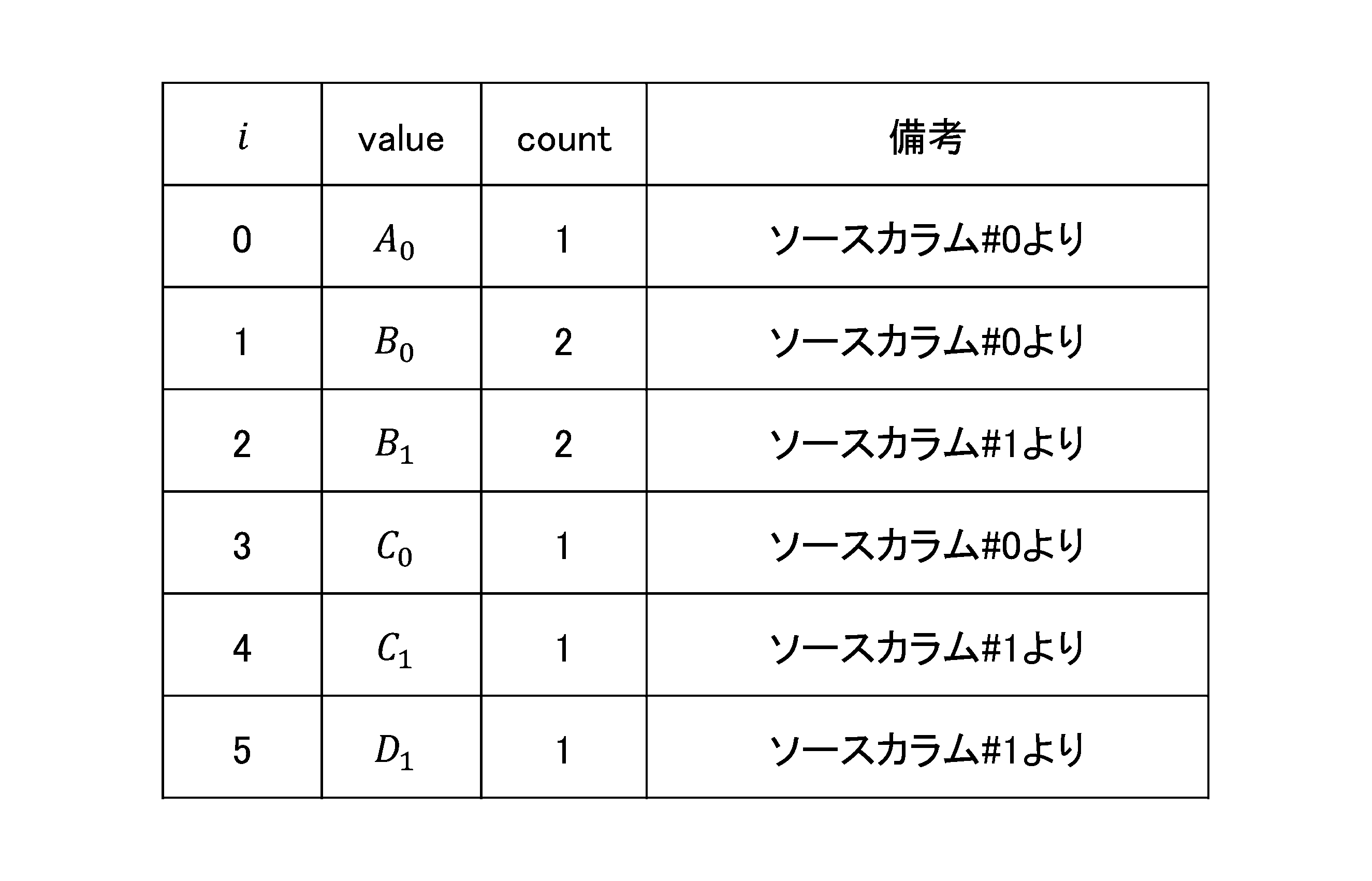
仮想転置構造体が階層的に作れることを述べたが、以下、実例を用いてそれを確かめる。図10は、D5AファイルであるC0(3)とC1(2)で仮想表形式データCV0(5)を作成し、その仮想表形式データCV0(5)とD5AファイルであるC2(3)で更なる仮想表形式データCV1(8)を作成する例を示している。以下に割り付け写像の定義を示す。
F(C1(2)→CV0(5))=(4,1)
F(CV0(5)→CV1(8))=(2,3,7,1,5)
F(C2(3)→CV1(8))=(0,6,4)
このとき、図10の転置構造体がどうなるのかを示したが図11である。C0(3)、C1(2)、CV0(5)、C2(3)の転置構造体又は仮想転置構造体は同図に示したとおりになる。それぞれのINVは式(15)と同様に、以下のようにしてINV'に読み替えられる。
INV1'=F(C1(2)→CV0(5))・INV1=(4,1)・(0,1)=(4,1)
INVV0'=F(CV0(5)→CV1(8))・INVV0=(2,3,7,1,5)・(3,4,2,0,1)=(1,5,7,2,3)
INV2'=F(C2(3)→CV1(8))・INV2=(0,6,4)・(2,1,0)=(4,6,0)
こうしてできたSVL、ACM、INV'を使って既に説明した手順によりCV0(5)、CV1(8)の仮想転置構造体が構成できる。
階層的にできた仮想転置構造体を用いた仮想インデックスでソートを行ってみる。図10、図11にはNNCが記載されていないためその代わりに図10のCV1(8)を用いる。ソート結果は以下となる。
上記の結果より確かにソートされていることが分かる。加えて、ソート結果には同じ「A」や「B」や「C」であってもC0(3)の「A」や「B」がC1(2)、C2(3)のそれらよりも先に来ることがわかる。これは同じ値のときはカラム番号が小さい方がその値が小さいとの取り決めが反映されたためである。また、ソート結果を保持するために新たな記憶領域を必要とすることがないのはD5Aインデックスと同じである。
階層的にできた仮想転置構造体を用いた仮想インデックスで検索を行ってみる。図10、図11にはNNCが記載されていないためその代わりに図10のCV1(8)を用いる。また、検索は「B」~「C」の条件で行うものとする。
また、検索結果を保持するためにはi0、i1を保持するだけでよいためわずかな記憶域しか必要としないことはD5Aインデックスと同じである。
階層的にできた仮想転置構造体を用いた仮想インデックスで集計を行ってみる。計結果のi番目の値valueは上記の情報2で与えられ、集計結果のi番目の値の出現回数countは式(8)で与えられる。それに従って集計を行うと、以下の表2のようになる。
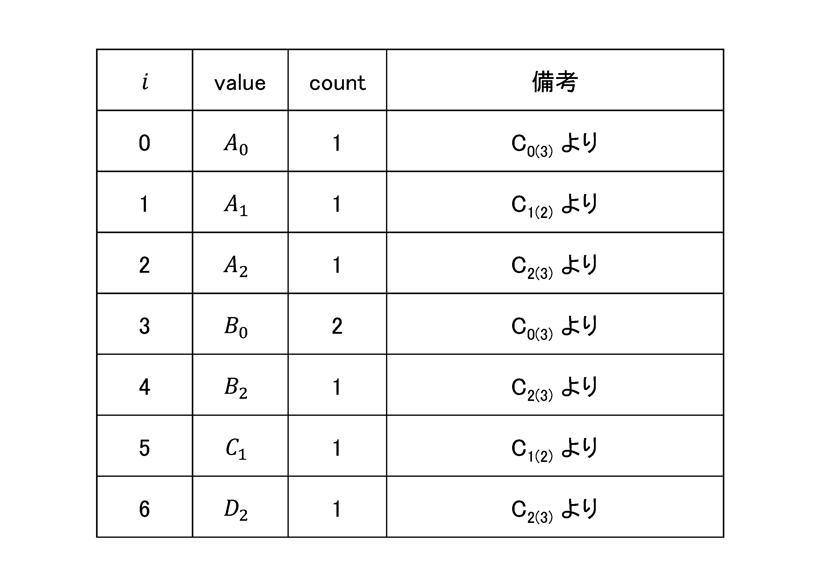
図11のC0(3),C1(2)→CV0(5)とCV0(5),C2(3)→CV1(8)をスペクトル分解の立場から解釈すると分かりやすい。分かりやすさのために、以下の式はすべて割り付け写像を使ってINVをINV'に読み替えた後の形で記載する。
C1(2)=A1:(4)+C1(1)
このため、CV0(5)は、以下で表すことができる。
また、CV0(5)とC2(3)をスペクトル分解で表すと以下となる。
C2(3)=A2:(4)+B2:(6)+D2:(0)
このため、CV1(8)は、以下で表すことができる。
したがって、ソート結果列は(1,5,4,7,2,6,3,0)となる。また、「B」
~「C」での検索結果列は(7,2,6,3)となる。集計も上記の表3と同様にできる。このため、手計算の場合はスペクトル分解による計算は分かりやすくて優れていることが分かる。
本実施形態に係るデータ処理装置10を含むシステムの全体構成例を図12に示す。図12に示すように、本実施形態に係るデータ処理装置10は、インターネット等のネットワーク20上に分散して配置されているデータベースサーバと通信可能に接続される。これらのデータベースサーバには、D5A又は仮想表形式データの少なくとも一方が1つ以上格納されている。
本実施形態に係るデータ処理装置10のハードウェア構成例を図13に示す。図13に示すように、本実施形態に係るデータ処理装置10は、入力装置201と、表示装置202と、外部I/F203と、通信I/F204と、RAM(Random Access Memory)205と、ROM(Read Only Memory)206と、補助記憶装置207と、プロセッサ208とを有する。これらの各ハードウェアは、それぞれがバス209を介して通信可能に接続される。
以下では、仮想表形式データの作成処理の流れについて、図14を参照しながら説明する。
以下では、仮想表形式データにおけるソート処理の流れについて、図15を参照しながら説明する。
以下では、仮想表形式データにおける検索処理の流れについて、図16を参照しながら説明する。
以下では、仮想表形式データにおける集計処理の流れについて、図17を参照しながら説明する。
以上のように、本実施形態に係るデータ処理装置10では、D5A又は既に定義済の仮想表形式データをソース表形式データとして、割り付け写像により新たな仮想表形式データを定義することができる。しかも、これらの仮想表形式データは仮想インデックスによりソート、検索、集計を高速に実現することが可能となる。
以下、補足として、既存技術ではインデックスの継承ができない一方で、本実施形態ではインデックスの継承が可能な理由について説明する。
20 ネットワーク
101 仮想表形式データ作成部
102 ソート部
103 検索部
104 集計部
105 記憶部
201 入力装置
202 表示装置
203 外部I/F
203a 記録媒体
204 通信I/F
205 RAM
206 ROM
207 補助記憶装置
208 プロセッサ
209 バス
Claims (19)
- 1以上の表形式データに含まれる1以上のカラムが持つ第1のデータ構造を所定の写像により変換した第2のデータ構造を持つ仮想カラムで構成される仮想表形式データに対して、前記第2のデータ構造をインデックスとして利用したソート操作、検索操作又は集計操作を行うデータ操作部、
を有するデータ処理装置。 - 前記1以上の表形式データには、前記第2のデータ構造を持つ仮想カラムで構成される仮想表形式データが含まれる、請求項1に記載のデータ処理装置。
- 前記1以上の表形式データには、前記カラムの値を昇順に保持する配列であるSVLと、前記カラムの値の転置レコード番号を保持する配列であるINVと、前記SVLと前記INVとの対応関係を保持する配列であるACMとで構成されるD5A、及び、前記仮想表形式データ、が含まれる、請求項1に記載のデータ処理装置。
- 前記1以上の表形式データには、前記カラムが更に含まれる、請求項3に記載のデータ処理装置。
- 前記1以上の表形式データには、前記カラムの値を前記SVL上の位置に置き換えた自然数を保持する配列であるNNCが更に含まれる、請求項3に記載のデータ処理装置。
- 前記データ操作部は、
前記仮想表形式データのソート対象のカラムに関する前記第2のデータ構造に含まれるINVにより、前記ソート対象のカラムの値を順に取得することで、前記ソート操作を行う、請求項3乃至5の何れか一項に記載のデータ処理装置。 - 前記データ操作部は、
前記仮想表形式データの検索対象のカラムに関する前記第2のデータ構造に含まれるINV及びACMと、検索条件として与えられた値v0及びv1とを用いて、v0≦SVL[i0]を満たす最小のi0とSVL[i1]≦i1を満たす最大のi1から(INV[ACM[i0-1]],・・・,INV[ACM[i1]-1])を検索結果として求めることで、前記検索操作を行う、請求項3乃至5の何れか一項に記載のデータ処理装置。 - 前記データ操作部は、
前記仮想表形式データの集計対象のカラムに関する前記第2のデータ構造に含まれるSVL及びACMを用いて、ACM[i]-ACM[i-1]により、前記仮想表形式データのSVLのi番目の要素の集計結果を算出することで、前記集計操作を行う、請求項3乃至5の何れか一項に記載のデータ処理装置。 - 1以上の表形式データに含まれる1以上のカラムが持つ第1のデータ構造を所定の写像により変換した第2のデータ構造を持つ仮想カラムで構成される仮想表形式データに対して、前記第2のデータ構造をインデックスとして利用したソート操作、検索操作又は集計操作を行うデータ操作手順、
をコンピュータが実行するデータ処理方法。 - 1以上の表形式データに含まれる1以上のカラムが持つ第1のデータ構造を所定の写像により変換した第2のデータ構造を持つ仮想カラムで構成される仮想表形式データに対して、前記第2のデータ構造をインデックスとして利用したソート操作、検索操作又は集計操作を行うデータ操作手順、
をコンピュータに実行させるプログラム。 - 作成対象の仮想表形式データのレコード数と、前記仮想表形式データのカラムを表す仮想カラムと、1以上の表形式データと、前記1以上の表形式データに含まれる1以上のカラムとの指定を受け付ける受付部と、
前記1以上の表形式データに含まれる前記1以上のカラムが持つ第1のデータ構造を所定の写像により変換した第2のデータ構造を前記仮想カラムに割り付けることで、前記仮想表形式データを作成する割り付け写像定義部と、
を有するデータ処理装置。 - 前記1以上のカラムの値を、前記仮想表形式データの前記仮想カラム上に表示する表示部、を有する請求項11に記載のデータ処理装置。
- 前記写像には、前記第1のデータ構造と前記第2のデータ構造との対応関係が1次関数で表現される1次関数型写像と、前記第1のデータ構造と前記第2のデータ構造との対応関係が前記対応関係の列挙で表現される列挙型写像とが含まれる、請求項11又は12に記載のデータ処理装置。
- 異なる第1のデータ構造に関して、異なる写像によりそれぞれ変換した第2のデータ構造が衝突するか否かを判定する衝突判定部、を有する請求項13に記載のデータ処理装置。
- 前記衝突判定部は、
前記異なる写像のうちの任意の2つの写像をF0,F1として、
前記写像F0の値域と前記写像F1の値域とが同一の仮想カラム上にない場合、前記写像F0の変換先の第2のデータ構造と前記写像F1の変換先の第2のデータ構造とは衝突しないと判定し、
前記写像F0の値域を表す区間の開始位置を表すインデックスをv0、前記写像F0の定義域を表す区間の長さをw0、前記写像F1の値域を表す区間の開始位置を表すインデックスをv1としたとき、v0+w0-1<v1である場合、前記写像F0の変換先の第2のデータ構造と前記写像F1の変換先の第2のデータ構造とは衝突しないと判定し、
前記写像F1の定義域を表す区間の長さをw1としたとき、v1+w1-1<v0である場合、前記写像F0の変換先の第2のデータ構造と前記写像F1の変換先の第2のデータ構造とは衝突しないと判定する、請求項14に記載のデータ処理装置。 - 前記衝突判定部は、
前記写像F0と前記写像F1とがいずれも列挙型写像である場合、前記写像F0の値域を表す区間の長さをw0、前記写像F1の値域を表す区間の長さをw1、L0=(v0,・・・,v0+w0-1)、L1=(v1,・・・,v1+w1-1)として、L0とL1の共通範囲L0',L1'を求め、各i,jに対してL0'[i]=L1'[j]とならないとき、前記写像F0の変換先の第2のデータ構造と前記写像F1の変換先の第2のデータ構造とは衝突しないと判定し、
前記写像F0と前記写像F1とがいずれも1次関数型写像である場合、前記写像F0の値域と前記写像F1の値域との共通部分を値域とするy0=a0×x0+b0;x0=0,1,2,・・・,N0-1で前記写像F0を記述し直すと共に、前記共通部分を値域とするy1=a1×x1+b1;x1=0,1,2,・・・,N1-1で前記写像F1を記述し直し、x0≦MinInt(N0-1,LCM(a0,a1)div a0)とx1≦MinInt(N1-1,LCM(a0,a1)div a1)のx0,x1に対してy0=y1とならないとき、前記写像F0の変換先の第2のデータ構造と前記写像F1の変換先の第2のデータ構造とは衝突しないと判定し、
前記写像F0が1次関数型写像、前記写像F1が列挙型写像である場合、前記写像F0の値域と前記写像F1の値域との共通部分を値域とするy0(n)=a0×n+b0;x0=0,1,2,・・・,N-1で前記写像F0を記述し直すと共に、前記共通部分を値域とするy1(m)=(v1,・・・,v1+w1-1)[m]で前記写像F1を記述し直し、各n,mに対してy0(n)=y1(m)とならないとき、前記写像F0の変換先の第2のデータ構造と前記写像F1の変換先の第2のデータ構造とは衝突しないと判定する、請求項15に記載のデータ処理装置。 - 前記第1のデータ構造及び前記第2のデータ構造は、転置レコード番号を要素とする配列を表すINVが少なくとも含まれるデータ構造である、請求項16に記載のデータ処理装置。
- 作成対象の仮想表形式データのレコード数と、前記仮想表形式データのカラムを表す仮想カラムと、1以上の表形式データと、前記1以上の表形式データに含まれる1以上のカラムとの指定を受け付ける受付手順と、
前記1以上の表形式データに含まれる前記1以上のカラムが持つ第1のデータ構造を所定の写像により変換した第2のデータ構造を前記仮想カラムに割り付けることで、前記仮想表形式データを作成する割り付け写像定義手順と、
をコンピュータが実行するデータ処理方法。 - 作成対象の仮想表形式データのレコード数と、前記仮想表形式データのカラムを表す仮想カラムと、1以上の表形式データと、前記1以上の表形式データに含まれる1以上のカラムとの指定を受け付ける受付手順と、
前記1以上の表形式データに含まれる前記1以上のカラムが持つ第1のデータ構造を所定の写像により変換した第2のデータ構造を前記仮想カラムに割り付けることで、前記仮想表形式データを作成する割り付け写像定義手順と、
をコンピュータに実行させるプログラム。
Priority Applications (5)
| Application Number | Priority Date | Filing Date | Title |
|---|---|---|---|
| JP2024572949A JPWO2024157776A1 (ja) | 2023-01-27 | 2024-01-11 | |
| CN202480009105.5A CN120584343A (zh) | 2023-01-27 | 2024-01-11 | 数据处理装置、数据处理方法及程序产品 |
| KR1020257027169A KR20250133955A (ko) | 2023-01-27 | 2024-01-11 | 데이터 처리 장치, 데이터 처리 방법, 및 프로그램 |
| EP24747107.1A EP4657274A4 (en) | 2023-01-27 | 2024-01-11 | DATA PROCESSING DEVICE, DATA PROCESS AND PROGRAM |
| US19/280,646 US20250355848A1 (en) | 2023-01-27 | 2025-07-25 | Data processing device, data processing method, and program |
Applications Claiming Priority (4)
| Application Number | Priority Date | Filing Date | Title |
|---|---|---|---|
| JP2023010717 | 2023-01-27 | ||
| JP2023-010717 | 2023-01-27 | ||
| JP2023-010716 | 2023-01-27 | ||
| JP2023010716 | 2023-01-27 |
Related Child Applications (1)
| Application Number | Title | Priority Date | Filing Date |
|---|---|---|---|
| US19/280,646 Continuation US20250355848A1 (en) | 2023-01-27 | 2025-07-25 | Data processing device, data processing method, and program |
Publications (1)
| Publication Number | Publication Date |
|---|---|
| WO2024157776A1 true WO2024157776A1 (ja) | 2024-08-02 |
Family
ID=91970355
Family Applications (1)
| Application Number | Title | Priority Date | Filing Date |
|---|---|---|---|
| PCT/JP2024/000399 Ceased WO2024157776A1 (ja) | 2023-01-27 | 2024-01-11 | データ処理装置、データ処理方法、及びプログラム |
Country Status (6)
| Country | Link |
|---|---|
| US (1) | US20250355848A1 (ja) |
| EP (1) | EP4657274A4 (ja) |
| JP (1) | JPWO2024157776A1 (ja) |
| KR (1) | KR20250133955A (ja) |
| CN (1) | CN120584343A (ja) |
| WO (1) | WO2024157776A1 (ja) |
Cited By (2)
| Publication number | Priority date | Publication date | Assignee | Title |
|---|---|---|---|---|
| US12536206B2 (en) * | 2024-05-08 | 2026-01-27 | Microsoft Technology Licensing, Llc | Inferring graph model from data in lake |
| US12547597B2 (en) | 2024-05-08 | 2026-02-10 | Microsoft Technology Licensing, Llc | Inferring graph model from semantic model |
Citations (3)
| Publication number | Priority date | Publication date | Assignee | Title |
|---|---|---|---|---|
| JP2013117873A (ja) * | 2011-12-02 | 2013-06-13 | Hitachi Systems Ltd | データベース処理方法 |
| JP2015207026A (ja) * | 2012-08-29 | 2015-11-19 | 株式会社ターボデータラボラトリー | 情報処理装置、レコード位置情報特定方法および情報処理プログラム |
| WO2023276162A1 (ja) * | 2021-07-02 | 2023-01-05 | 晋二 古庄 | データ作成装置、データ作成方法、及びプログラム |
Family Cites Families (7)
| Publication number | Priority date | Publication date | Assignee | Title |
|---|---|---|---|---|
| JPH1091644A (ja) * | 1996-09-10 | 1998-04-10 | Oki Electric Ind Co Ltd | データベース問い合わせ処理方法及び装置 |
| JP3860992B2 (ja) * | 2001-11-09 | 2006-12-20 | 株式会社ターボデータラボラトリー | データの結合・提示方法、および、データ結合・提示プログラム |
| JP4881435B2 (ja) * | 2007-06-21 | 2012-02-22 | 株式会社ターボデータラボラトリー | メモリ共有型並列処理システムにおいて表形式データを集計する方法及び装置 |
| US10237916B2 (en) | 2015-09-30 | 2019-03-19 | Tokyo Electron Limited | Systems and methods for ESC temperature control |
| CA3038475A1 (en) | 2016-09-28 | 2018-04-05 | Immpact-Bio Ltd. | A universal platform for car therapy targeting a novel antigenic signature of cancer |
| JP2021067962A (ja) * | 2018-02-21 | 2021-04-30 | 株式会社ターボデータラボラトリー | 情報処理システム及び情報処理方法 |
| CN116648697A (zh) * | 2021-01-13 | 2023-08-25 | Ess控股株式会社 | 信息处理方法、信息处理装置和程序 |
-
2024
- 2024-01-11 JP JP2024572949A patent/JPWO2024157776A1/ja active Pending
- 2024-01-11 CN CN202480009105.5A patent/CN120584343A/zh active Pending
- 2024-01-11 WO PCT/JP2024/000399 patent/WO2024157776A1/ja not_active Ceased
- 2024-01-11 KR KR1020257027169A patent/KR20250133955A/ko active Pending
- 2024-01-11 EP EP24747107.1A patent/EP4657274A4/en active Pending
-
2025
- 2025-07-25 US US19/280,646 patent/US20250355848A1/en active Pending
Patent Citations (3)
| Publication number | Priority date | Publication date | Assignee | Title |
|---|---|---|---|---|
| JP2013117873A (ja) * | 2011-12-02 | 2013-06-13 | Hitachi Systems Ltd | データベース処理方法 |
| JP2015207026A (ja) * | 2012-08-29 | 2015-11-19 | 株式会社ターボデータラボラトリー | 情報処理装置、レコード位置情報特定方法および情報処理プログラム |
| WO2023276162A1 (ja) * | 2021-07-02 | 2023-01-05 | 晋二 古庄 | データ作成装置、データ作成方法、及びプログラム |
Non-Patent Citations (1)
| Title |
|---|
| See also references of EP4657274A1 * |
Cited By (2)
| Publication number | Priority date | Publication date | Assignee | Title |
|---|---|---|---|---|
| US12536206B2 (en) * | 2024-05-08 | 2026-01-27 | Microsoft Technology Licensing, Llc | Inferring graph model from data in lake |
| US12547597B2 (en) | 2024-05-08 | 2026-02-10 | Microsoft Technology Licensing, Llc | Inferring graph model from semantic model |
Also Published As
| Publication number | Publication date |
|---|---|
| EP4657274A1 (en) | 2025-12-03 |
| EP4657274A4 (en) | 2026-04-15 |
| US20250355848A1 (en) | 2025-11-20 |
| CN120584343A (zh) | 2025-09-02 |
| JPWO2024157776A1 (ja) | 2024-08-02 |
| KR20250133955A (ko) | 2025-09-09 |
Similar Documents
| Publication | Publication Date | Title |
|---|---|---|
| Anand et al. | Mining of massive datasets | |
| JP5342958B2 (ja) | 圧縮データの構造を問い合わせる方法 | |
| US8533203B2 (en) | Identifying synonyms of entities using a document collection | |
| Amato et al. | MI-File: using inverted files for scalable approximate similarity search | |
| US7761407B1 (en) | Use of primary and secondary indexes to facilitate aggregation of records of an OLAP data cube | |
| US8219564B1 (en) | Two-dimensional indexes for quick multiple attribute search in a catalog system | |
| Genuzio et al. | Fast scalable construction of (minimal perfect hash) functions | |
| US20250355848A1 (en) | Data processing device, data processing method, and program | |
| CN113536040B (zh) | 信息查询方法、装置以及存储介质 | |
| Deepak et al. | EvoMiner: frequent subtree mining in phylogenetic databases | |
| Khan et al. | Set-based unified approach for summarization of a multi-attributed graph | |
| Baswana et al. | Mincut sensitivity data structures for the insertion of an edge | |
| US11106703B1 (en) | Clustering of structured and semi-structured data | |
| Brisaboa et al. | Aggregated 2d range queries on clustered points | |
| Chen et al. | On the signature tree construction and analysis | |
| Karaoglu et al. | The number of cubic surfaces with 27 lines over a finite field | |
| Aggarwal et al. | Gconnect: A connectivity index for massive disk-resident graphs | |
| Patil et al. | Succinct representations of weighted trees supporting path queries | |
| JP2004534981A (ja) | データベース・システムでデータを編成し、問合せを処理する方法、およびそのような方法を実施するためのデータベース・システムおよびソフトウェア製品 | |
| McKay et al. | Enumeration of Latin squares with conjugate symmetry | |
| Yang et al. | Querying a collection of continuous functions | |
| Harvey et al. | Resolving unresolved resolved and unresolved triplets consistency problems | |
| Chen et al. | On the Designing of Popular Packages | |
| Paul et al. | Optimized entity attribute value model: a search efficient representation of high dimensional and sparse data | |
| JP2021114037A (ja) | インデックス管理装置 |
Legal Events
| Date | Code | Title | Description |
|---|---|---|---|
| 121 | Ep: the epo has been informed by wipo that ep was designated in this application |
Ref document number: 24747107 Country of ref document: EP Kind code of ref document: A1 |
|
| DPE1 | Request for preliminary examination filed after expiration of 19th month from priority date (pct application filed from 20040101) | ||
| ENP | Entry into the national phase |
Ref document number: 2024572949 Country of ref document: JP Kind code of ref document: A |
|
| WWE | Wipo information: entry into national phase |
Ref document number: 2024572949 Country of ref document: JP |
|
| WWE | Wipo information: entry into national phase |
Ref document number: 202480009105.5 Country of ref document: CN |
|
| ENP | Entry into the national phase |
Ref document number: 1020257027169 Country of ref document: KR Free format text: ST27 STATUS EVENT CODE: A-0-1-A10-A15-NAP-PA0105 (AS PROVIDED BY THE NATIONAL OFFICE) |
|
| WWE | Wipo information: entry into national phase |
Ref document number: 1020257027169 Country of ref document: KR |
|
| NENP | Non-entry into the national phase |
Ref country code: DE |
|
| WWP | Wipo information: published in national office |
Ref document number: 202480009105.5 Country of ref document: CN |
|
| WWP | Wipo information: published in national office |
Ref document number: 2024747107 Country of ref document: EP |