Disclosure of Invention
Aiming at the defects of the prior art, the invention provides a rail transit passenger flow prediction method which is high in prediction accuracy based on time sequence characteristics.
In order to achieve the purpose, the invention adopts the following technical scheme: a rail transit passenger flow volume prediction method based on space-time characteristics comprises the following steps:
s1, collecting historical data of rail transit passenger flow;
s2, extracting the spatial characteristics and the time sequence characteristics of the target station from 0 to t from the historical data collected in the step S1;
s3, synthesizing the spatial features and the time sequence features of the historical data of the target station at the time 0 to t in the step S2 into a two-dimensional vector of the target station at the time 0 to t correspondingly;
and S4, establishing an LSTM artificial neural network model, training the LSTM artificial neural network model by taking the two-dimensional vector of the target station from 0 to t as input, and then inputting the two-dimensional vector of the target station at t into the trained LSTM artificial neural network model to obtain the outbound passenger flow of the target station at t + 1.
As an improvement, in step S1, historical data of rail transit passenger flow is collected, and the historical data is described using the following formula:
xy,t,in=∑i∈M{i|i.otime∈t;i.ostation=j} (1-1);
xj,t,out=∑i∈M{i|i.dtime∈t;i.dstation=j} (1-2);
wherein i represents a piece of data in the whole track traffic data set M, and the otime, dtime, attitude and dstation are attributes of the data i and respectively represent the card swiping time for entering the station, the card swiping time for exiting the station, the number of the starting station and the number of the terminal station.
As an improvement, the spatial characteristics of the target station at time 0 to t in step S2 are calculated by the following method:
wherein: sj,rThe total number of passenger flows of other stations which are going to reach the target station j at the moment r, namely the spatial characteristics of the target station at the moment r;
n is the set of rail transit total network stations;
n represents the total data volume of the site set N;
Pk,j,rthe space association factor refers to the space association factor of a station k and a target station j at the moment r at the moment t;
Ink,t-ΔTrepresenting the number of the arrival people of the station k in the r-delta T time period;
Δ T is the average travel time difference between site k and target site j;
wherein, Ink,t-ΔTRepresenting the number of the arrival people of the station k in the r-delta T time period;
i represents one piece of data in the whole track traffic data set M;
m represents the total data volume of the track traffic data set M;
xk,j,r-ΔTthe representative is the r- Δ T time period, the number of people in the passenger flow from station k to destination station j;
w represents a time period;
Pk,j,rthat is, all historical contemporaneous p at time rk,j,rAverage value of (a).
As an improvement, the timing characteristics of the target station from 0 to t in step S2 are obtained by the following method:
Tj,r=(tj,rtj,r-1…tj,r-time_step)T (3);
wherein, Tj,rThe total number of outbound passenger flows of a target station j in a historical time period at r moment;
tj,rthe number of the people who go out of the target site j at the moment r is represented;
time step represents a time step.
As an improvement, in step S3, the spatial feature and the temporal feature of the target station at time 0 to time t are correspondingly synthesized into the two-dimensional vector Input of the target station at time 0 to time tj,tThe following were used:
as an improvement, the LSTM artificial neural network model established in step S4 is as follows:
ar=σ(Wa,r·xr+ba,r) (4-1);
fr=σ(Wf,r·[hr-1,ar]+bf,r) (4-2);
ir=σ(Wi,r·[hr-1,ar]+bi,r) (4-3);
or=σ(Wo,r·[hr-1,ar]+bo,r) (4-6);
hr=or*tanh(Cr) (4-7);
wherein, arIndicating full link layer output at time r, Wa,rRepresenting full connection layer weight at time r, ba,rDenotes the offset of the fully-connected layer at time r, xrAn input representing time r;
frrepresents the forgetting threshold at time r, hr-1Representing the output of the cell at time r-1, Wf,rRepresenting the weight of forgetting to gate at time r, bf,rA bias indicating a forgetting gate at time r;
irrepresenting the input threshold at time r, Wi,rRepresenting entry gate weight at time r, bi,rRepresents the offset of the input gate at time r;
new state, W, of cell generation at time r
c,rRepresents the weight of the cell at time r, b
C,rRepresenting the bias of the cell at the r moment;
representing the cell state at the r-1 moment;
Crrepresenting the total state of the cell at the r moment;
orrepresenting the output threshold at time r, Wo,rRepresenting the weight of the output gate at time r, bo,rRepresents the offset of the output gate at time r;
hrindicating the output at time r.
As an improvement, the training process of the LSTM artificial neural network model established in step S4 is as follows:
1) let r be 1;
2) two-dimensional vector Inputj,rAs input, i.e. order xr=Inputj,rAnd performing the calculation of the following relation:
ar=σ(Wa,r·xr+ba,r) (4-1);
fr=σ(Wf,r·[hr-1,ar]+bf,r) (4-2);
ir=σ(Wi,r·[hr-1,ar]+bi,r) (4-3);
or=σ(Wo,r·[hr-1,ar]+bo,r) (4-6);
hr=or*tanh(Cr) (4-7);
3) when r > t, executing the next step, otherwise, making r equal to r +1, and returning to 2);
and outputting the current LSTM artificial neural network model, wherein the model is the trained LSTM artificial neural network model.
As an improvement, in step S3, the two-dimensional vector of the target site at time t is used as an input, and the trained LSTM artificial neural network model is input, that is, let x ber=t=Inputj,tThen output hj=t=yt+1;
yt+1And the predicted result, namely the predicted outbound passenger flow of the target station j at the time of the rail transit t +1 is shown.
The invention has the following beneficial effects:
the invention innovatively introduces two dimensionality characteristics of rail transit, namely time characteristics and space characteristics, combines the two dimensionality characteristics to form a two-dimensional vector, trains an LSTM artificial neural network model by taking the two-dimensional vector of the target station at 0-t as input, and predicts the outbound passenger flow of the target station at t +1 time by taking the two-dimensional vector of the target station at t as input, and has high prediction precision.
Detailed Description
In order to make the objects, technical solutions and advantages of the present invention more apparent, the present invention will be described in further detail with reference to the accompanying drawings in conjunction with the following detailed description. It should be understood that the description is intended to be exemplary only, and is not intended to limit the scope of the present invention. Moreover, in the following description, descriptions of well-known structures and techniques are omitted so as to not unnecessarily obscure the concepts of the present invention.
The rail transit data has space-time two-dimension.
The timeliness is as follows: the passenger flow data in a certain time period has a certain rule, and the data in adjacent time periods have a certain correlation.
Spatiality: there is a spatial relationship between the two sites. Every two different sites have certain rules in the traffic of different time periods.
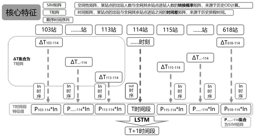
Due to the fact that the rail transit data is spatial besides temporal, a certain correlation exists between every two stations in space, and the most direct embodiment of the correlation is the travel time of a passenger. The spatial relationship between the two sites can be expressed by converting the spatial distance between the two sites into the travel time, namely the time difference delta T. In addition, for a given time period, the traffic volume between every two stations has a certain rule, and the relation is introduced by introducing a space influence factor matrix SIM.
In the framework provided by the invention, the space influence quantity is converted into the time difference to be processed, so that the spatiality can be processed by an artificial neural network for processing time series data. The time sequence data and the space influence quantity are combined to predict the station entering and exiting data of the station, and a good effect is obtained.
Referring to fig. 1 and 2, a rail transit passenger flow volume prediction method based on space-time characteristics includes the following steps:
s1, collecting historical data of rail transit passenger flow;
specifically, historical data of rail transit passenger flow is collected, and the historical data is described by using the following formula:
xj,t,in=∑i∈M{i|i.otime∈t;i.ostation=j} (1-1);
xj,t,out=∑i∈M{i|i.dtime∈t;i.dstation=j} (1-2);
wherein i represents a piece of data in the whole track traffic data set M, and the otime, dtime, attitude and dstation are attributes of the data i and respectively represent the card swiping time for entering the station, the card swiping time for exiting the station, the number of the starting station and the number of the terminal station.
S2, extracting the spatial characteristics and the time sequence characteristics of the target station from 0 to t from the historical data collected in the step S1;
specifically, the spatial feature of the target station at time 0 to t in step S2 is calculated by the following method:
wherein: sj,rThe total number of passenger flows of other stations which are going to reach the target station j at the moment r, namely the spatial characteristics of the target station at the moment r;
n is the set of rail transit total network stations;
n represents the total data volume of the site set N;
Pk,j,rthe space association factor refers to the space association factor of a station k and a target station j at the moment r at the moment t;
Ink,t-ΔTrepresenting the number of the arrival people of the station k in the r-delta T time period;
Δ T is the average travel time difference between site k and target site j; the Δ T between every two stations constitutes a T matrix, which is described in detail below), and all P form an SIM matrix (which is described in detail below), that is, a transition probability matrix (time period, ratio of the number of inbound people from station k to station j to the total number of inbound people from station k) of the outbound people of the target station j to the number of inbound people of the rest stations in the whole network.
Wherein, Ink,t-ΔTRepresenting the number of the arrival people of the station k in the r-delta T time period;
i represents one piece of data in the whole track traffic data set M;
m represents the total data volume of the track traffic data set M;
xk,j,r-ΔTthe representative is the r- Δ T time period, the number of people in the passenger flow from station k to destination station j;
w represents a time period;
Pk,j,rthat is, all historical contemporaneous p at time rk,j,rAverage value of (a).
History synchronization: the same time period of each week, such as 8 o 'clock 30 of Monday on all weeks, constitutes a historical contemporaneous group of 8 o' clock 30 of Monday, noting that: here, 8 points 30 points refers to a period of time, which represents 8: 21-8 points 30. This time is 10 minutes because the prediction accuracy in our experiment is 10 minutes, and if the prediction accuracy is v, the time period t refers to the time period t-v to t.
Specifically, the time sequence characteristics of the target station at time 0 to t are obtained by the following method:
Tj,r=(tj,rtj,r-1…tj,r-time_step)T (3);
wherein, Tj,rThe total number of outbound passenger flows of a target station j in a historical time period at r moment;
tj,rthe number of the people who go out of the target site j at the moment r is represented;
time step represents a time step. The constants in the LSTM neural network are specified by the user as specific values.
S3, synthesizing the spatial features and the time sequence features of the historical data of the target station at the time 0 to t in the step S2 into a two-dimensional vector of the target station at the time 0 to t correspondingly;
specifically, in step S3, the spatial feature and the time sequence feature of the target site at time 0 to time t are correspondingly synthesized into the two-dimensional vector Input of the target site at time 0 to time tj,tThe following were used:
namely, a two-dimensional vector with the length of time step is used as the input of an LSTM artificial neural network model, the processing of a full connection layer is carried out, and the Output of the full connection layer is OutputfullAn input as an input layer; finally, a one-dimensional vector with the length of 1 is output. The output is the predicted value of the total number of passenger flows of the destination station j. The output of the LSTM artificial neural network model is a specific number.
Multiple experiments show that the two-dimensional vector is adopted as a station with small input and output number and large data fluctuation, and the performance is generally good.
S4: establishing an LSTM artificial neural network model, training the LSTM artificial neural network model by taking the two-dimensional vector corresponding to the time from 0 to t as input, and then inputting the two-dimensional vector corresponding to the time t into the trained LSTM artificial neural network model to obtain the outbound passenger flow of the target station at the time t + 1.
Specifically, the LSTM artificial neural network model established in step S4 is as follows:
ar=σ(Wa,r·xr+ba,r) (4-1);
fr=σ(Wf,r·[hr-1,ar]+bf,r) (4-2);
ir=σ(Wi,r·[hr-1,ar]+bi,r) (4-3);
or=σ(Wo,r·[hr-1,ar]+bo,r) (4-6);
hr=or*tanh(Cr) (4-7);
wherein, arIndicating full link layer output at time r, Wa,rRepresenting full connection layer weight at time r, ba,rDenotes the offset of the fully-connected layer at time r, xrAn input representing time r;
frrepresents the forgetting threshold at time r, hr-1Representing the output of the cell at time r-1, Wf,rRepresenting the weight of forgetting to gate at time r, bf,rA bias indicating a forgetting gate at time r;
irrepresenting the input threshold at time r, Wi,rRepresenting entry gate weight at time r, bi,rRepresents the offset of the input gate at time r;
new state, W, of cell generation at time r
c,rRepresents the weight of the cell at time r, b
C,rRepresenting the bias of the cell at the r moment;
representing the cell state at the r-1 moment;
Crrepresenting the total state of the cell at the r moment;
orrepresenting the output threshold at time r, Wo,rRepresenting the weight of the output gate at time r, bo,rRepresents the offset of the output gate at time r;
hrindicating the output at time r.
Adding a full connection layer before the input layer of the traditional LSTM artificial neural network, wherein the full connection layer has the function of connecting the above
The vector of [ time _ step, 2] is converted into a vector of [ time _ step, rnn _ unit ] (rnn _ unit is the number of cells, constant in the LSTM neural network, specific values given by the user), and the converted vector is input into the input layer of the LSTM.
Specifically, the training process of the LSTM artificial neural network model established in step S4 is as follows:
1) let r be 1;
2) two-dimensional vector Inputj,rAs input, i.e. order xr=Inputj,rAnd performing the calculation of the following relation:
ar=σ(Wa,r·xr+ba,r) (4-1);
fr=σ(Wf,r·[hr-1,ar]+bf,r) (4-2);
ir=σ(Wi,r·[hr-1,ar]+bi,r) (4-3);
or=σ(Wo,r·[hr-1,ar]+bo,r) (4-6);
hr=or*tanh(Cr) (4-7);
3) when r > t, executing the next step, otherwise, making r equal to r +1, and returning to 2);
and outputting the current LSTM artificial neural network model, wherein the model is the trained LSTM artificial neural network model. The two-dimensional vector synthesized in the step S3 is used as the input in the step S4 to train the LSTM artificial neural network model to obtain Wa,r、ba,r、Wf,r、bf,r、Wi,r、bi,r、Wc,r、bC,r、Wo,rAnd bo,rAnd determining the trained LSTM artificial neural network model.
In the step S3, the two-dimensional vector of the target site at the time t is used as input, and the trained LSTM artificial neural network model is input, namely, x is orderedr=t=Inpuj,tThen output hj=r=yt+1;
yt+1And the predicted result, namely the predicted outbound passenger flow of the target station j at the time of the rail transit t +1 is shown.
The model takes time characteristic data and space characteristic data as input and outputs outbound passenger flow data at the future moment. The input time characteristic and space characteristic data innovatively introduce the characteristics of two dimensions of rail transit, namely time characteristic and space characteristic. And combining the time characteristic and the space characteristic to form a two-dimensional vector as the input of the model, wherein the output is the outbound passenger flow at the time of the target station t + 1.
The structure of the T matrix is as follows:
Ttrepresented is a time difference matrix T for the T period.
ΔTk,jRepresenting a history of time differences from site k to site j for time period tAverage of the term of the same term (and calculate P)k,j,tHistorical averaging method of time is the same):
(i∈M,i.dtime∈t,i.ostation=k,i.dstation=j)
Δtk,j,trepresented is the average travel time from station k to station j at time t.
ΔTk,j,tIs the delta t of all historical synchronizationk,j,tW in the formula represents one week.
N is the set of full-network sites, which is 122 sites in the full network, i.e., m-122.
H is a set of all time segments, each day is 7 days a week, subway operation is 1000 minutes each day, and the time segment length (prediction accuracy) is 10 minutes, so that there are 7 × 1000/10-700 time segments in total.
For a given time period T, a T matrix is corresponded, the size of the matrix is the station number by the station number (122 by 122, the total network is 122 stations), and the travel time of the time period T between every two stations in the total network is described. In the prediction experiment, there were 100 time periods in a day. It has also been found that the travel time for each site varies from day to day, but is cycled roughly on a weekly cycle (with different travel times between sites throughout the network from monday to sunday). Therefore, we have a total of 7 x 100T matrices, each with a size of 122 x 122.
The structure of the SIM matrix is as follows:
SIMtthe spatial impact factor matrix SIM at time t is represented.
Pk,jRepresented is the historical contemporaneous average of the spatial impact factors for site k to site j at time t.
N is the set of full-network sites, which is 122 sites in the full network, i.e., m-122.
H is a set of all time segments, each day is 7 days a week, subway operation is 1000 minutes each day, and the time segment length (prediction accuracy) is 10 minutes, so that there are 7 × 1000/10-700 time segments in total.
For a given time t, the method corresponds to an SIM matrix, the size of the matrix is the station number (122 station number, 122 station numbers in the whole network), and the correlation degree between every two stations in the whole network and the number of the station entering people and the number of the battle exiting people at the time t is depicted. In the prediction experiment, there were 100 time periods in a day. Moreover, the relevance rules of the number of the coming-in persons and the number of the coming-out persons at two stations are different from day to day, but the rules are approximately circulated in a week period (the relevance rules are different between every two stations in the whole network from Monday to Sunday). Therefore, we have a total of 7 × 100 SIM matrices, each with a size of 122 × 122.
Test of
Experimental data set and experimental subject
A data source: whole-network rail transit card swiping data of Chongqing city of 3 months in 2017
Prediction of objects: number of people who come out of 100 rail transit stations in Chongqing
Precision: 10 minutes
Data volume: each station has incoming passenger flow data and outgoing passenger flow data, and each station has 100 × 30 × 2 (1000/10) × 600000 data, wherein training is performed on the first 28 days and testing is performed on the last 2 days.
Training times are as follows: 3000 times.
Testing the model: conventional models that predict only from time to time data, and spatio-temporal prediction models that incorporate the amount of spatial impact.
Accuracy measure index
1) Maximum error
The maximum value of the absolute values of the differences between the predicted value and the actual value in the prediction result.
2) Mean error
In the prediction result, the absolute value of the difference between the predicted value and the actual value is averaged.
3) Root mean square error
In the prediction result, the sum of squares of absolute values of the differences between the predicted value and the actual value is set to the square.
4) Relative accuracy
The average percentage of the absolute value of the difference between the predicted value and the actual value in the prediction result.
Test results
| Model name
|
Maximum error
|
Mean error
|
Root mean square error
|
Relative accuracy
|
| Two-dimensional input space-time prediction model
|
127.90
|
19.06
|
27.87
|
83.81%
|
| Time sequence prediction model
|
182.88
|
24.81
|
37.51
|
79.16% |
Conclusion of the experiment
After the experiment of 100 sites, the space-time prediction model of the two combination modes has good performance, each index is obviously higher than that of the traditional time sequence prediction model, and the prediction accuracy is obviously improved.
To prevent the loss of meaning indicated by the letters, the following list is made:
the above description is only an embodiment of the present invention, but the scope of the present invention is not limited thereto, and any person skilled in the art can easily conceive of changes or substitutions within the technical scope of the present invention, and all such changes or substitutions are included in the scope of the present invention. Therefore, the protection scope of the present invention shall be subject to the protection scope of the claims.