CN112116830A - Unmanned aerial vehicle dynamic geo-fence planning method based on airspace meshing - Google Patents

Abstract

The invention discloses a dynamic geo-fence planning method for unmanned aerial vehicles based on low-altitude airspace gridding. Based on the flexible track prediction results, the longitudinal length dimension of the dynamic geofence is designed; the historical track data within the target airspace is preprocessed, and the airspace is uniformly gridded and numbered; the key indicators affecting the complexity of the low-altitude airspace are defined , using the kernel K-means clustering method to perform clustering analysis on the airspace grid to achieve the results of hierarchical measurement of low-altitude airspace complexity; combined with the low-altitude airspace grid complexity, the horizontal range planning of dynamic geofence dynamic geofence is carried out. This method is the first to propose a complete set of UAV dynamic geofencing planning method and apply it to low-altitude airspace air traffic management, which can effectively improve the utilization rate of low-altitude airspace and help alleviate the shortage of low-altitude airspace resources.

Description

Unmanned aerial vehicle dynamic geo-fence planning method based on airspace meshing

Technical Field

The invention relates to an air traffic planning management technology, in particular to an unmanned aerial vehicle dynamic geo-fence planning method based on airspace meshing.

Background

With the continuous deepening of the application of civil unmanned aerial vehicles and the rapid expansion of the market of the unmanned aerial vehicles, the operation management of low-altitude airspace in the future faces huge challenges. On one hand, as for the air traffic management mode of the low-altitude airspace, the mode of dividing and isolating the airspace or the mode of planning a static geo-fence under the traditional management mode is a relatively extensive management mode, and the busy airspace resources caused by economic or geographic factors cannot meet the requirements. On the other hand, the management mode of the low-altitude airspace cannot be divided into sector control modes according to the sector of the transport airspace due to various types, sizes and flight modes of the aircraft in the low-altitude airspace. Therefore, the air traffic management mode of the low-altitude airspace should be combined with the characteristics of the air traffic management mode, and reasonable planning is carried out aiming at the problems of airspace resource shortage, potential conflict among unmanned aerial vehicles and the like.

Disclosure of Invention

The purpose of the invention is as follows: the invention aims to provide an unmanned aerial vehicle dynamic geo-fence planning method based on airspace meshing, and solves the practical problems of low-altitude airspace resource shortage, low utilization rate and the like caused by the existing low-altitude airspace traffic management modes such as partitioning and isolating airspace or static geo-fence planning and the like.

The technical scheme is as follows: the invention discloses an unmanned aerial vehicle dynamic geo-fence planning method based on low-altitude airspace meshing, which comprises the following steps of:

s1, considering the randomness characteristic of the actual flight path of the unmanned aerial vehicle, and performing flexible flight path prediction on the flight plan of the unmanned aerial vehicle;

s2, designing the longitudinal length dimension of the dynamic geo-fence by combining the flexible track prediction result of the unmanned aerial vehicle;

s3, preprocessing historical track data in a target airspace range, and uniformly meshing and numbering the airspaces;

s4, defining key indexes influencing the complexity of the low-altitude space domain, and performing clustering analysis on the space domain grid by adopting a kernel K-mean clustering method to realize a low-altitude space domain complexity grading measurement result;

and S5, combining the low-altitude spatial domain grid complexity to carry out dynamic geofence lateral range planning.

Further, step S1 is specifically:

firstly, considering the performance of the unmanned aerial vehicle and flight plan data, comprehensively calculating a horizontal track, a height profile and a speed profile, and thus obtaining an initial 4D (three-dimensional) track of the unmanned aerial vehicle; on the basis, the random characteristics of the actual track of the unmanned aerial vehicle are considered, namely the uncertainty of the wind speed and the instability of the indicated airspeed cause the difference between the actual average ground speed and the calculated result;

suppose that the indicated airspeed V of the drone is in the cruise phase_TASAnd wind speed V_WSAll obey a normal distribution with indicated airspeed

Wind speed

The probability density function is respectively:

the average groundspeed V can be known by combining the characteristics of normal distribution and the expression of the average groundspeed_GSSubject to a normal distribution, i.e.

And the probability density function is:

from this calculate unmanned aerial vehicleThe actual value of the average airspeed in a certain flight section is in the range of mu +/-3 sigma, namely

Further, step S2 is specifically:

under the comprehensive influence of flight habits and wind speeds, the average ground speed of the unmanned aerial vehicle at the moment t is [ mu ]_GS-3σ_GS,μ_GS+3σ_GS]Within range, then the longitudinal length of the corresponding dynamic geofence

Comprises the following steps:

therefore, the longitudinal length of the unmanned aerial vehicle dynamic geofence is 6t sigma_GSMeanwhile, the planning time step increases, which accords with the basic fact that the uncertainty increases when planning for a long time.

Further, step S3 is specifically:

selecting historical track data in a target airspace, preprocessing the historical track data, and removing abnormal data, data in a non-target airspace range and track point data in a non-low-altitude airspace; then, converting the target airspace into a plane rectangular coordinate system according to the mercator projection, and then uniformly discretizing the target airspace on the plane coordinate system to obtain uniform airspace grids on a two-dimensional plane and numbering the uniform airspace grids; then, analyzing historical track data in a Broadcast type Automatic Dependent Surveillance-Broadcast (ADS-B) format to obtain original index data of each airspace grid; numbering; the coordinate origin is taken as a starting point, the main direction is sequentially increased in the x-axis direction, and the secondary direction is sequentially increased in the y-axis direction; meanwhile, knowing the unit length of each grid airspace, the lower left corner coordinate of each grid is taken to represent the grid corner mark.

Further, step S4 is specifically:

s41, introducing track historical data on the basis of airspace meshing, and taking track density, track point speed distribution, track point height distribution, machine type mixing degree, potential conflict degree, obstacle exceeding height and track time density as key indexes influencing low-altitude airspace complexity; processing the key indexes by adopting a linear weighting method to obtain a comprehensive evaluation value of the grid airspace complexity, namely a comprehensive evaluation model of the complexity; the linear weighting method is:

and S42, combining high-dimensional characteristics and comprehensive evaluation results of multiple complexity influence indexes of the unit grid, introducing a kernel function theory, and combining a K-means clustering algorithm to carry out hierarchical quantitative research on the complexity of the spatial domain grid.

Firstly, processing a multi-index comprehensive quantization result, determining the number K of cluster classes according to an actual problem, equally dividing a sample into K parts according to the total number m of the sample, and marking the K parts as C ═ C₁,c₂,…,c_KTaking the median of the comprehensive quantized value in each sample as an initial clustering center; then mapping the original data to a high-dimensional feature space through nonlinear transformation, and then carrying out K-means clustering in the feature space;

given the total number of samples in the selected spatial grid m, the sample set is { g }⁽¹⁾,g⁽²⁾,…,g^(m)In which g is⁽ⁱ⁾∈G^N1,2, 3.. m, according to Mercer's theorem, if the mapping Φ is known:

so that K (g)⁽ⁱ⁾,g^(j))＝Φ(g⁽ⁱ⁾)^TΦ(g^(j))，K(g⁽ⁱ⁾,g^(j)) Can be used to represent a kernel function where G^NIs a selected spatial grid sample g⁽ⁱ⁾Space in, G^FIs a selected spatial grid sample g⁽ⁱ⁾Phi (g) obtained by mapping phi⁽ⁱ⁾) The space in which the device is located; benefit toChanging the distribution form of the sample by using a kernel function without knowing the concrete representation form of the sample in a mapping high-dimensional space; kernel K-means clustering is just to discuss the original sample set g⁽¹⁾,g⁽²⁾,…,g^(m)Data set { phi (g) obtained after phi is mapped⁽¹⁾),Φ(g⁽²⁾),…,Φ(g^(m)) At G^FClustering conditions in space; the distance from the ith sample in sample space to the kth class center is:

sequencing the samples in sequence by the comprehensive quantization value, and preliminarily dividing the complexity levels of the samples according to the set complexity level quantity and the sample proportion of each level; and then mapping the samples to a high-dimensional kernel space, and taking the mean value of the comprehensive quantization values of the samples of each complexity level as an initial clustering center.

Further, step S5 is specifically:

s51, solving a target predicted track point;

predicting track points of the unmanned aerial vehicle target based on the unmanned aerial vehicle flexible track prediction technology provided in S1;

s52, solving a basic grid airspace set;

coordinates P of two track points_start(x₀,y₀) And P_end(x₁,y₁) Solving an expression y of a two-point connecting line as rx + b according to a linear equation; first by calculating Δ x ═ x₀-x₁| and Δ y ═ y₀-y₁L to determine the primary direction of movement:

if Δ x>Δ y, which indicates that the maximum difference value of the x-axis is greater than the maximum difference value of the y-axis, and the x-axis direction is the main direction of movement; if Δ x<Δ y, which indicates that the maximum difference value of the y axis is greater than the maximum difference value of the x axis, and the y axis direction is the main direction of movement; rounding the coordinates of the starting point to the side length of the grid respectively, i.e. ordering

Where a is the grid edgeLength;

when the x-axis is the main direction of movement, the current point is P'_start(x′₀,y′₀) Wherein x'₀＝ai，y′₀Aj, when x ═ x'₀At + a, y ═ k (x'₀+ a) + b, by rounding y down with the grid side length,

let σ be y '-y'₀And then:

computing

After step, when x ═ x'₁That is, when the end point is located in the grid, the outsourced grid space domain set G where the connecting line of the start point and the end point is located is obtained_baseThe same applies when the y-axis is the main direction of movement;

s53, solving an expanded space domain by a sliding neighborhood method;

let S be the initial solution, i.e. the basic spatial domain set, and the number of neighborhoods be M, N_lRepresenting the ith neighborhood. When neighborhood searching is carried out, if S is optimized after the current neighborhood searching is finished, namely the benefit function is increased, the current neighborhood is added into the optimal solution, the next neighborhood structure is operated, otherwise, the operation is stopped, and the current solution is output;

obtaining a grid airspace set G through which a track point connecting line passes according to an rounding method_baseIn the order of G_baseAs an initial solution S; sequentially translating the initial solution to two sides for M times to obtain M increasing neighborhoods which are used as a neighborhood structure set and respectively recorded as N₁,N₂,…,N_M；

The search order between the neighborhood structures can be changed by changing the order between the neighborhood structures, and generally, the search order is ordered according to the size of the neighborhood, namely: n is a radical of₁(x)≤N₂(x)≤N₃(x)≤…≤N_max(x) (ii) a According to the actual situation, the sequence among the neighborhood structures is in a way of sequentially crossing and arranging towards two sides by taking the initial solution as a reference.

S54, defining a benefit function F_objRepresenting the maximum benefit of a grid airspace distributed in a certain planning stage, wherein the airspace set consists of a basic airspace and an extended airspace, and the basic airspace and the extended airspace are respectively a grid airspace where a track center line is located and a part of grid airspace adjacent to the grid airspace; by f_disRepresenting the benefit of the degree of freedom brought by increasing the current extended space domain, f_cRepresents the negative complexity benefit, g, of the grid space domain generation_ijThe decision variables represent that when the total benefit brought by adding a certain grid is positive, the grid is divided into an expanded airspace, and the benefit function expression is as follows:

because the target is a course operation plan, considering that a grid which is too far away from a course point connecting line has no practical significance for planning a geo-fence, a continuous grid airspace set with lower complexity grade tends to be searched near a predicted course, namely, the reciprocal of the distance between a current airspace grid and a straight line where the predicted course is located is adopted to represent the benefit of the degree of freedom:

mu is a parameter with adjustable degree of freedom, d is the distance between the current airspace grid and a straight line where a predicted flight path is located, s is a complexity value, lambda is used for ensuring that when the airspace grid is planned, the grid too far away from a flight path cannot be planned into a planning queue even if the complexity is low, the value of lambda is set according to the actual condition, sigma is used for adjusting the influence of the complexity to bring negative benefits according to the actual requirement, and the value of sigma is set according to the actual condition;

since the benefit of freedom function is a single branch in the first quadrant of the hyperbola, the benefit of freedom f increases with distance d_disWill be gradually reduced in size and will be gradually reduced,setting mu as a freedom degree adjustable parameter, when d is larger than mu, the benefit of the freedom degree is less than 1, meanwhile, because the complexity value is represented by the weighted average value of the normalized index data, considering that the influence degrees of all indexes on the complexity are the same, the value range of the complexity value is s ∈ [0,1 ∈]When λ is 1.5 μ and σ is 1, f is_c∈[1,1.5μ+1]When d is greater than μ, the benefit function F_obj≤0；

The model constraint conditions are as follows:

the decision variable is a 0-1 variable and represents whether the current grid is in the optimal solution set or not, and when g is_ijWhen 1, it means that the optimal solution set contains the current mesh, when g_ijWhen the number is 0, the current grid is not included;

g_ij＝0,1；

as a precondition for completing a flight mission by an unmanned aerial vehicle, a basic grid airspace is required to meet the requirement of the current flight mission, and a grid where a starting point and a terminal point connecting line are located is required to be an optimal solution set in a model;

g_ij1 (if g)_ij∈G_base)；

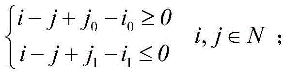
Restricting the range of the feasible region, if the grids of the start point and the end point are respectively g_i0j0And g_i1j1When the slope r of the straight line of the starting point and the end point is<At time 0:

when the slope r > 0:

when the slope r is 0:

i₀≤i≤i₁,i,j∈N；

in the absence of slope r:

j₀≤j≤j₁,i,j∈N；

and (3) connectivity constraint, knowing that the linear equation of the connecting line of the starting point and the end point is that Ax + By + C is 0, wherein a and B are not 0 at the same time, when Ai + Bj + C is less than or equal to 0, namely the grid is located below the connecting line:

when Ai + Bj + C is more than or equal to 0, namely the grid is positioned below the connecting line:

and S55, calculating whether the benefit function of the basic spatial domain grid is positive by using the spatial domain complex hierarchical measurement method provided by S4 and the benefit function provided by S54, if so, indicating that the basic spatial domain grid set slides to two sides in sequence, and if not, outputting all the expanded spatial domain grid sets.

Has the advantages that: compared with the prior art, the invention provides a set of complete unmanned aerial vehicle dynamic geo-fence planning method based on airspace meshing for the first time, overcomes the defects of airspace resource distribution modes such as planning static geo-fences and planning isolated airspaces, and self-adaptively adjusts the size of the geo-fence through time slot distribution and low-altitude airspace complexity, so that busy low-altitude airspace resources with higher airspace complexity are utilized more carefully, accurately and efficiently, and meanwhile, the idle low-altitude airspace with lower complexity is utilized to increase the spatial freedom and safety of flight activities of the unmanned aerial vehicle. Therefore, the dynamic geo-fencing planning of the unmanned aerial vehicle can achieve the purpose of reasonably distributing low-altitude airspace resources to a certain extent, and has very important significance in promoting a fine management mode of the low-altitude airspace.

Drawings

Fig. 1 is a schematic flow diagram of a dynamic geofence planning process for an unmanned aerial vehicle;

FIG. 2 is a schematic diagram of a dynamic geofence vertical dimension design process in the present invention;

FIG. 3 is a schematic diagram of a low-altitude spatial domain complexity hierarchical metric model;

fig. 4 is a schematic diagram of the dynamic geofence lateral coverage planning process of the present invention.

Detailed Description

The present invention will be further described with reference to the accompanying drawings.

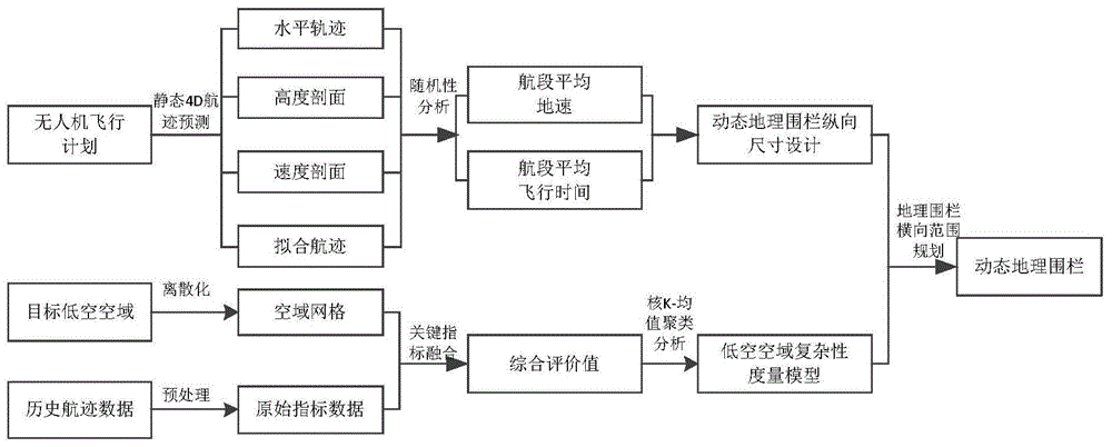
Fig. 1 is a flow chart of the present invention, which may specifically include the following steps:

s1, considering the randomness characteristic of the actual flight path of the unmanned aerial vehicle, and performing flexible flight path prediction on the flight plan of the unmanned aerial vehicle;

for a target flight plan, firstly, an unmanned aerial vehicle initial static 4D track model is established by combining unmanned aerial vehicle performance parameters, then, track randomness characteristics of the unmanned aerial vehicle in actual flight are analyzed, the unmanned aerial vehicle initial 4D track model is improved according to the track randomness characteristics, and finally, a flexible 4D track prediction model is generated.

The model for predicting the initial static 4D flight path of the unmanned aerial vehicle is specifically as follows: the 4D track refers to an accurate description of the flight path of the aircraft continuously from the current position to the end position based on four dimensions, and each point on the 4D track is accurately associated with time. The 4D flight path research of the transport aviation is to improve the air traffic safety and the air traffic efficiency, and mainly takes the flight path management of an aircraft as a center, and improves the utilization rate and the safety of airspace and airport resources by accurately arranging the flight path and the time of the aircraft; the 4D track prediction model mainly comprises a) horizontal track generation; b) a fly height profile; c) a flight speed profile and d) initial track generation.

a) Horizontal trajectory generation: the horizontal track of the unmanned aerial vehicle refers to the projection of the track of the unmanned aerial vehicle in the whole flight task on the horizontal plane. As the flight principle of the fixed-wing unmanned aerial vehicle can be known, the unmanned aerial vehicle cannot hover and turn when the course is adjusted, and horizontal turning maneuver needs to be carried out, the actual flight path of the unmanned aerial vehicle is formed by a curve and a straight line segment together. When the range of the unmanned aerial vehicle is long and the length of the straight line segment is far greater than that of the circular arc, the curve during turning can be properly ignored, and the horizontal track is composed of pure straight line segments. When the requirement on the accuracy of the flight path is high, the flight path curve of the unmanned aerial vehicle during turning needs to be considered,

b) flight height profile: the flight height profile of the unmanned aerial vehicle is the projection of a flight path from takeoff to landing of the unmanned aerial vehicle on a plumb surface in a rectangular spatial coordinate system. The flight height profile of the climbing stage can calculate the flight height of each waypoint at a time interval or a flight distance interval according to the climbing rate or climbing gradient of the unmanned aerial vehicle; the flying height is kept unchanged in the cruising stage; and the flight height profile of the descending stage takes the height of the cruising stage as the initial height, and is calculated according to the descending rate and the descending gradient.

c) Flight speed profile: the flight speed profile of the unmanned aerial vehicle refers to the rule that the speed of the unmanned aerial vehicle changes along with the course. Because the research object of the invention is the fixed-wing unmanned aerial vehicle which carries out flying operation in a low-altitude airspace, on the premise that the flying height does not change much, the influence of the flying height is ignored, and the indicated airspeed is approximately equal to the vacuum speed. The typical flight speed profile of the unmanned aerial vehicle is generally divided into three stages, namely an acceleration stage, a constant speed stage and a deceleration stage, the unmanned aerial vehicle needs to accelerate at a certain acceleration under the condition that the unmanned aerial vehicle performance allows before reaching the cruise indication airspeed, and then the unmanned aerial vehicle keeps at a constant speed to fly flatly until the unmanned aerial vehicle needs to decelerate.

d) Initial track generation: the geographical coordinates of each route point are generated according to the horizontal track, the time required from the current route point to the next route point can be calculated according to the speed profile information, the distance between the route points and the wind field information, the time of the unmanned aerial vehicle passing through each route point can be obtained from the first route point, and the initial static 4D route prediction of the unmanned aerial vehicle can be realized by combining the flight height profile of the unmanned aerial vehicle

The flexible 4D track prediction model of the unmanned aerial vehicle is as follows: in the actual flight process, because both can't guarantee that unmanned aerial vehicle strictly follows the flight of maximum cruising speed, simultaneously because wind produces certain interference to unmanned aerial vehicle chance, lead to actual flight and ideal condition to have some errors. Therefore, the value range of the average ground speed of the unmanned aerial vehicle in each flight segment is obtained according to the '3 sigma principle' by comprehensively considering the normal distribution characteristic of the average ground speed, and a more reasonable position range where the unmanned aerial vehicle is located at the current moment is obtained.

As shown in fig. 2, first, the performance of the drone and flight plan data are considered, and a horizontal trajectory, an altitude profile and a speed profile are comprehensively calculated, so as to obtain an initial 4D track of the drone. On the basis, the random characteristics of the actual track of the unmanned aerial vehicle, namely uncertainty of wind speed and instability of indicated airspeed, are considered, so that the difference between the actual average ground speed and the calculated result is generated.

Suppose that the indicated airspeed V of the drone is in the cruise phase_TASAnd wind speed V_WSAll obey a normal distribution with indicated airspeed

Wind speed

The probability density function is respectively:

wherein, mu_TASRepresenting the mean indicated airspeed, σ_TASMeans indicating standard deviation of airspeed, μ_WSRepresenting the mean value of the wind speed, σ_WSIndicating the standard deviation of wind speed. The average groundspeed V can be known by combining the characteristics of normal distribution and the expression of the average groundspeed_GSSubject to a normal distribution, i.e.

And the probability density function is:

therefore, the actual value of the average airspeed of the unmanned aerial vehicle in a certain flight section can be calculated within the range of mu +/-3 sigma, namely

Wherein DA is a drift angle and represents the deviation degree of the flight path line and the course line, and WA is a wind angle and represents the included angle between the wind direction line and the flight path line.

S2, designing the longitudinal length dimension of the dynamic geo-fence by combining the flexible track prediction result of the unmanned aerial vehicle;

as shown in fig. 2, the normal distribution characteristic of the average ground speed is comprehensively considered, so that the method for calculating the longitudinal length of the dynamic geofence is optimized and adjusted to obtain a more reasonable position range of the unmanned aerial vehicle at the current moment, and according to the flexible track prediction result, the longitudinal length of the corresponding dynamic geofence can be obtained by knowing the average ground speed range and the average flight time of the unmanned aerial vehicle at a certain moment. Under the comprehensive influence of flight habits and wind speeds, the average ground speed of the unmanned aerial vehicle at the moment t is [ mu ]_GS-3σ_GS,μ_GS+3σ_GS]Within range, then the longitudinal length of the corresponding dynamic geofence

Comprises the following steps:

therefore, the longitudinal length of the unmanned aerial vehicle dynamic geofence is 6t sigma_GSMeanwhile, the planning time step increases, which accords with the basic fact that the uncertainty increases when planning for a long time. Wherein, mu_GSRepresenting the mean ground speed, σ_GSRepresenting the standard deviation of the ground speed.

The method comprises the steps of selecting a certain type of fixed wing unmanned aerial vehicle to carry out case simulation in the process of cargo transportation activities, selecting a certain processed flight plan as a specific analysis object, wherein the information comprises a plan number P-20191201-1, a plan time 12:00, and waypoints 1 and 2, and the longitude and latitude coordinates of the air route are (31.5,119) and (31.8,119.2), respectively. And analyzing the flight sections of the two route points, and obtaining the predicted flight path and flight section flight time of the unmanned aerial vehicle on the flight section according to the initial flight path generation method.

When the unmanned aerial vehicle flies on the flight segment in a single direction, assuming that the distribution law of the indicated airspeed and the wind speed on the current flight segment is known, the distribution parameters of the average ground speed can be obtained according to Monte Carlo simulation, and meanwhile, the flight path can be calculated according to the longitude and latitude of two route points, so that the average flight time of the flight segment is calculated to be 0.322 h. The ground speed of the drone obeys a normal distribution with mean 119.792, variance 16.752, maximum 135.034, and minimum 101.621.

Defining dynamic geofence lengthener L_CDI.e., the length of the drone fence in the heading direction, is expressed as the difference between the smaller of the two, the forwardmost end of the dynamic geofence and the destination waypoint, and the largest of the two, the rear end of the dynamic geofence and the starting waypoint. Taking the planning step length tau as 5s, and calculating L of each planning time on the flight segment when the speed range method is adopted_CDThat is, the longitudinal length of the fence is calculated in the speed range of the drone performance, and then the dynamic geofence lengthenerity is considered in the context of track randomness

The comparative results are shown in Table 1.

TABLE 1

It can be seen from the table that

Less than L_CDNamely, the adopted dynamic geographic fence longitudinal length planning method saves airspace resources more, and in the actual planning, the planning step length tau can be reasonably adjusted according to the requirement, especially in the initial planning stage

Shorter, can suitably increase the step length in order to guarantee unmanned aerial vehicle safe flight.

S3, preprocessing historical track data in a target airspace range, and uniformly meshing and numbering the airspaces;

as shown in fig. 3, the historical track data in the target airspace is selected first, and then the historical track data is preprocessed to remove abnormal data, data in a non-target airspace range and track point data in a non-low-altitude airspace. Then, converting a target low-altitude airspace geographic coordinate system into a planar rectangular coordinate system according to the mercator projection, then uniformly discretizing the target low-altitude airspace on the planar rectangular coordinate system in a certain division level to obtain uniform airspace grids on a two-dimensional plane, and then analyzing and processing historical track data in a Broadcast type Automatic Dependent Surveillance-Broadcast (ADS-B) format to obtain original index data of each airspace grid; and numbered. The coordinate origin is taken as a starting point, the primary direction is sequentially increased in the x-axis direction, and the secondary direction is sequentially increased in the y-axis direction. Meanwhile, knowing the unit length of each grid airspace, the lower left corner coordinate of each grid is taken to represent the grid corner mark.

S4, defining key indexes influencing the complexity of the low-altitude space domain, and performing clustering analysis on the space domain grid by adopting a kernel K-mean clustering method to realize a low-altitude space domain complexity grading measurement result;

as shown in fig. 3, the method comprises the following steps:

s41, track historical data are introduced on the basis of airspace meshing, and track density, track point speed distribution, track point height distribution, model mixing degree, potential conflict degree, obstacle exceeding height and track time density are used as key indexes influencing low-altitude airspace complexity. And processing the key indexes by adopting a linear weighting method to obtain a comprehensive evaluation value of the grid airspace complexity, namely a comprehensive evaluation model of the complexity. The linear weighting method is:

wherein, CR_iIs the comprehensive evaluation value of the ith grid space domain complexity, omega_jIs the weight of the j index, F'_jIs the evaluation value of the jth index, and n represents the influence of the selectionThe number of key indexes of low-altitude space domain complexity.

According to the result after the index normalization, the complexity relative value CR of the ith grid space domain can be calculated_iLet n indices in the vector be considered equally weighted, then ω is_jAll get

Otherwise ω is_jDifferent values can be taken according to the importance degree of the current index.

And S42, combining high-dimensional characteristics and comprehensive evaluation results of multiple complexity influence indexes of the unit grid, introducing a kernel function theory, and combining a K-means clustering algorithm to carry out hierarchical quantitative research on the complexity of the spatial domain grid.

Firstly, processing a multi-index comprehensive quantization result, determining the number K of cluster classes according to an actual problem, equally dividing a sample into K parts according to the total number m of the sample, and marking the K parts as C ═ C₁,c₂,…,c_KAnd taking the median of the comprehensive quantized values in each sample as an initial clustering center. Therefore, the clustering result has better comprehensive quantitative value grading characteristics. And then mapping the original data to a high-dimensional feature space through nonlinear transformation, and then carrying out K-means clustering in the feature space.

Given the total number of samples in the selected spatial grid m, the sample set is { g }⁽¹⁾,g⁽²⁾,…,g^(m)}. Wherein g is⁽ⁱ⁾∈G^N1,2, 3. According to Mercer's theorem, if the mapping Φ is known:

so that K (g)⁽ⁱ⁾,g^(j))＝Φ(g⁽ⁱ⁾)^TΦ(g^(j))，K(g⁽ⁱ⁾,g^(j)) It can be used to represent a kernel function where G^NIs a selected spatial grid sample g⁽ⁱ⁾Space in, G^FIs a selected spatial grid sample g⁽ⁱ⁾Phi (g) obtained by mapping phi⁽ⁱ⁾) The space in which the device is located. The distribution form of the sample is changed by utilizing the kernel function without knowing the characteristics of the sample in the mapping high-dimensional spaceThe body represents the form. Kernel K-means clustering is just to discuss the original sample set g⁽¹⁾,g⁽²⁾,…,g^(m)Data set { phi (g) obtained after phi is mapped⁽¹⁾),Φ(g⁽²⁾),…,Φ(g^(m)) At G^FClustering conditions in space. The distance from the ith sample in sample space to the kth class center is:

and sequencing the samples sequentially by the comprehensive quantization value, and preliminarily dividing the complexity levels of the samples according to the set complexity level quantity and the sample proportion of each level. And then mapping the samples to a high-dimensional kernel space, and taking the mean value of the comprehensive quantization values of the samples of each complexity level as an initial clustering center. The clustering result obtained by the method can ensure that the comprehensive quantization value of each cluster is in a certain range, the comprehensive quantization value of each cluster basically presents gradient distribution, a better complexity grading effect can be obtained by only processing the cross repeated part and the outlier, and the establishment of a complexity grading measurement model is realized. The result gives consideration to the high-dimensional structural characteristics of the comprehensive quantized value and the original index data, and has better practical significance.

ADS-B data of 7, 23 and 7 months in 2019 of a certain airport are selected for case simulation, and the data are preprocessed firstly. Selecting a 50km low-altitude airspace range around an airport, wherein the latitude is about 34.9506292053 to 35.8544246137, the longitude is 118.789668151 to 119.870509340, converting a geographic coordinate system of a target airspace (same altitude layer, and the deviation of upper and lower boundary bands of the same altitude layer is ignored) represented by the latitude and the longitude of WGS _84 standard into a mercator projection plane rectangular coordinate system, translating a coordinate origin to O ' for convenience of calculation, namely, translating x ' -x-O (x) and y ' -y (y) to obtain a plane rectangular coordinate system taking a lower left corner coordinate of the target airspace range as the origin, wherein x and y are coordinates of a midpoint of the original plane rectangular coordinate system on an x axis and a y axis, x ' and y ' are coordinates of the midpoint of the translated plane rectangular coordinate system on the x axis and the y axis, and O (x) and O (y) are translation lengths along the x axis and the y axis respectively. Uniformly dividing a target airspace range under a rectangular coordinate system into unit grid airspaces of 30 multiplied by 30, numbering each airspace grid, processing ADS-B historical track data of three natural days of the airport, removing abnormal data, data in a non-target airspace range and track point data in a non-low-altitude airspace range, and corresponding the track points and the grids one by one according to position information. The track point data of 900 airspace grids are obtained through preliminary processing, then the comprehensive quantitative value calculation is carried out on the original data of each grid step by step, 900 groups of data lists with 8 complexity indexes are obtained, and partial results are shown in table 2.

TABLE 2

In order to present the complexity level layering condition of a target airspace, the obtained standardized index data is considered to be subjected to cluster analysis, and the comprehensive quantification result of the index is not considered, so that the analysis is carried out only by adopting the traditional K-means clustering method. And carrying out K-means method clustering analysis by using Python, and obtaining 6 non-uniform clusters by using Euclidean distance between influence indexes of complexity of each grid airspace as a clustering basis. And after the clustering results correspond to the actual target airspace grids, obtaining the distribution of the complexity degree of the low-altitude airspace near the airport. However, the clustering method can only reflect the sample characteristics with similar complexity contained in multiple indexes, and if complexity grade division needs to be performed between different classes, the original index data of the sample serving as a clustering center needs to be further analyzed. In order to make up the unicity defect of the expression complexity of the comprehensive evaluation quantitative value and the defect that the traditional clustering analysis method cannot better perform quantitative grading, the index data is processed by adopting a kernel K-mean clustering method, so that the clustering result comprises the comprehensive evaluation quantitative result. Firstly, carrying out primary processing on samples, sequencing 900 samples according to the index comprehensive evaluation value from small to large, uniformly dividing the sequenced samples into 6 groups, taking a grid sample point to which the median of the comprehensive evaluation index of each group of samples belongs as an initial clustering center, and obtaining the result shown in table 3.

TABLE 3

Then, a Gaussian kernel function is selected to represent the high-dimensional space distance of the two sample points, and finally, a clustering analysis result is obtained. Through analysis, results obtained by adopting a kernel K-means clustering method generate a better grading effect on complexity distribution. The complexity degree is also overlapped in a small part among various types, because the essence of the clustering algorithm is that the distance of a high-dimensional kernel space is considered preferentially, although the comprehensive evaluation indexes of the sample points are relatively close, the high-dimensional space structure of the original index data has certain difference, and the result also indicates that the complexity degree of a grid airspace cannot be reflected comprehensively by simply considering the weighted average value of multiple indexes from the side, so the complexity description is more scientific and complete by adopting the method of combining the comprehensive quantitative value and the high-dimensional space clustering.

S5, planning the dynamic geofence transverse range by combining the low-altitude airspace grid complexity;

and according to the longitudinal length planning result of the dynamic geo-fence, taking the current track point and the next track point as the planning basis, marking all unit grid airspaces passing through the connection line of the two track points as basic airspaces, reasonably marking a plurality of unit grid airspaces with lower airspace complexity adjacent to the basic airspace as extended airspaces, and forming the transverse airspace range of the unmanned aerial vehicle dynamic geo-fence in the period with the basic airspaces.

As shown in fig. 4, the dynamic geofence lateral range planning method specifically includes the following steps:

s51, solving a target predicted track point;

predicting track points of the unmanned aerial vehicle target based on the unmanned aerial vehicle flexible track prediction technology provided in S1;

s52, solving a basic grid airspace set;

the coordinates of the starting point and the end point of the unmanned aerial vehicle are respectively P_start(x₀,y₀) And P_end(x₁,y₁) The expression y of the two-point connection line is obtained as rx + b according to the straight-line equation. First by calculating Δ x ═ x₀-x₁| and Δ y ═ y₀-y₁L to determine the primary direction of movement:

if Δ x>Δ y, which indicates that the maximum difference value of the x-axis is greater than the maximum difference value of the y-axis, and the x-axis direction is the main direction of movement; if Δ x<And deltay, namely the maximum difference value of the y axis is larger than that of the x axis, and the y axis direction is the main direction of movement. Rounding the coordinates of the starting point to the side length of the grid respectively, i.e. ordering

Where a is the grid side length, then P_start(x₀,y₀) At g_ijThe spatial grid represented.

When the x-axis is the main direction of movement, the current point is P'_start(x′₀,y′₀) Wherein x'₀＝ai，y′₀Aj, when x ═ x'₀At + a, y ═ k (x'₀+ a) + b, by rounding y with the side length of the grid downwards,

let σ be y '-y'₀And then:

computing

After step, when x ═ x'₁That is, when the grid of the end point is located, the outsourced grid space domain set G where the connecting line of the start point and the end point is located can be obtained_baseThe same applies when the y-axis is the primary direction of movement.

S53, solving an expanded space domain by a sliding neighborhood method;

let S be the initial solution, i.e. the basic spatial domain set, and the number of neighborhoods be M, N₁Representing the ith neighborhood. When neighborhood searching is carried out, if S is optimized after the current neighborhood searching is finished, namely the benefit function is increased, the current neighborhood is added into the optimal solution, operation is carried out on the next neighborhood structure, otherwise, the operation is stopped, and the current solution is output.

Obtaining a grid airspace set G through which a track point connecting line passes according to an rounding method_baseIn the order of G_baseAs the initial solution S. Sequentially translating the initial solution to two sides for M times to obtain M increasing neighborhoods which are used as a neighborhood structure set and respectively recorded as N₁,N₂,…,N_M；

The search order between the neighborhood structures can be changed by changing the order between the neighborhood structures, and generally, the search order is ordered according to the size of the neighborhood, namely: n is a radical of₁(x)≤N₂(x)≤N₃(x)≤…≤N_max(x) In that respect According to the actual situation, the sequence among the neighborhood structures is in a way of sequentially crossing and arranging towards two sides by taking the initial solution as a reference. The choice of the stopping criterion has a direct and important impact on both the algorithm global convergence and timeliness.

S54, defining a benefit function F_objAnd representing the maximum total benefit of the grid airspace distributed in a certain planning stage, wherein the airspace set consists of a basic airspace and an extended airspace, and the basic airspace and the extended airspace are respectively a grid airspace where the track center line is located and a part of grid airspace adjacent to the grid airspace. By f_disRepresenting the benefit of the degree of freedom brought by increasing the current extended space domain, f_cRepresents the negative complexity benefit, g, of the grid space domain generation_ijA decision variable, which means that when the total benefit brought by adding a certain grid is positive, the grid is divided into an expanded space domainThe beneficial function expression is:

the N is the number of the grids in the feasible regions in the x-axis direction and the y-axis direction, and because the target is the operation planning of the air route, and considering that the grids which are too far away from the connecting line of the track point have no practical significance to the planning of the geo-fence, a continuous grid airspace set with lower complexity grade tends to be searched near the predicted track, namely, the reciprocal of the distance between the current airspace grid and the straight line where the predicted track is located is adopted to express the benefit of the degree of freedom:

mu is a parameter with adjustable degree of freedom, d is the distance between the current airspace grid and the straight line where the predicted flight path is located, s is a complexity value, lambda is used for ensuring that when the airspace grid is planned, the grid too far away from the air route does not be planned into a planning queue even if the complexity is low, the value of lambda is set according to the actual condition, sigma is used for adjusting the influence of the complexity to bring negative benefits according to the actual requirement, and the value of sigma is set according to the actual condition.

Since the benefit of freedom function is a single branch in the first quadrant of the hyperbola, the benefit of freedom f increases with distance d_disAnd gradually reducing, setting mu as a freedom degree adjustable parameter, and when d is greater than mu, setting the freedom degree benefit to be less than 1, wherein the meaning is that the airspace too far away from the predicted air route has no practical help to the flight of the airspace, namely the contribution of the freedom degree benefit to the total benefit value tends to 0. Meanwhile, the complexity value is represented by the weighted average of the normalized index data, and the value range of the complexity value is s ∈ [0,1 ] considering that the influence degree of all indexes on the complexity is the same]When λ is 1.5 μ and σ is 1, f is_c∈[1,1.5μ+1]When d is greater than μ, the benefit function F_obj≤0。

Meanwhile, the practical significance of the benefit function also means that the requirement on the complexity of the grid is lower and lower along with the gradual increase of the distance between the expanded airspace grid and the predicted flight path, and the grid airspace near the predicted flight path can appropriately relax the requirement on the complexity level so as to ensure that the airspace distributed for the grid can meet the requirement on safe flight. Combining with the actual situation, the constraint conditions of the benefit function model are as follows:

the decision variable is a 0-1 variable and represents whether the current grid is in the optimal solution set or not, and when g is_ijWhen 1, it means that the optimal solution set contains the current mesh, when g_ijIf 0, the current grid is not included.

g_ij＝0,1；

As a precondition for completing a flight mission by an unmanned aerial vehicle, a basic grid airspace is required to meet the requirement of the current flight mission, and a grid where a starting point and a terminal point connecting line are located is required to belong to an optimal solution set in a benefit function model.

g_ij1 (if g)_ij∈G_base)；

Wherein G is_baseIs the outsourced grid airspace set where the starting point and the end point connecting line are located.

Restricting the range of the feasible region if the starting point and the end point are respectively positioned at g_i0j0And g_i1j1Spatial grid of representations i₀And j₀Subscript, i, indicating the grid number at which the start point is located₁And j₁Subscript indicating the grid number of the end point, i and j indicate subscripts indicating the grid number of the feasible region, when the straight line of the start point and the end point is

When the slope r < 0:

when the slope r > 0:

when the slope r is 0:

i₀≤i≤i₁,i,j∈N；

in the absence of slope r:

j₀≤j≤j₁,i,j∈N；

and (3) connectivity constraint, knowing that the linear equation of the connecting line of the starting point and the end point is that Ax + By + C is 0(a and B are not 0 at the same time), when Ai + Bj + C is less than or equal to 0, namely the grid is positioned below the connecting line:

when Ai + Bj + C is more than or equal to 0, namely the grid is positioned below the connecting line:

wherein, g_i,j+1Is a decision variable, g, corresponding to the spatial grid with index (i, j +1)_i+1,jIs a decision variable, g, corresponding to the spatial grid with index (i +1, j)_i-1,jIs a decision variable, g, corresponding to the spatial grid with index (i-1, j)_i,j-1Is a decision variable corresponding to the spatial grid with subscript (i, j-1),

and S55, calculating whether the benefit function of the basic spatial domain grid is positive by using the spatial domain complex hierarchical measurement method provided by S4 and the benefit function provided by S54, if so, indicating that the basic spatial domain grid set slides to two sides in sequence, and if not, outputting all the expanded spatial domain grid sets.

Selecting a low-altitude airspace within 50km of a certain airport square circle as a planning target, converting the geography of two track points (35.6078399956,119.4278243855) and (35.6322514834,119.5232603629) into rectangular coordinates according to a coordinate conversion method, and obtaining a result P_start(71039.227,89620.1935) and P_end(81663.1114,92963.1438), taking the unit grid space domain length as

Rounding a downwards to obtain the grid number g of the a_17,22And g_20,23Then, a basic spatial domain grid set G is obtained through calculation_base. First, the equation of a straight line between two points is obtained from the coordinates of the two points as f (x) is 0.3146x +67266.7306 since | k<1, so that x can be determined as the main moving direction, i.e. G can be obtained by only calculating 20-17+1 to 4 steps_base。

When m is equal to 0, the compound is,

when m is 1, the coordinates of the starting point are normalized to obtain P'_start(68000,88000) increasing x by one grid unit length to obtain x₁72000, mixing x₁Substituting into linear equation to obtain y₁Get y rounded down to 89922.5138₁' 88000, calculate σ_0,1＝y′₁-y′₀0, according to the solving formula of the basic grid space domain set,

by analogy, it can be calculated that when m is 4,

then solving the extended spatial domain grid set G according to the variable neighborhood method_expIn this example, the main movement direction is the x-axis, and k>0, the upper neighborhood can be calculated

Lower neighborhood

Then, according to the complexity value of each grid and the distance to the predicted flight path, calculating a benefit function F of each neighborhood_objObtaining a final assigned airspace grid set

The specific trellis encoding results are shown in table 4.

TABLE 4

The invention discloses an unmanned aerial vehicle dynamic geo-fence planning method based on low-altitude airspace grid complexity. According to the method, on the basis of low-altitude airspace meshing, a low-altitude airspace complexity measurement model with key influence indexes such as track density, speed fluctuation and altitude change is established, and a flexible 4D (four-dimensional) track prediction model is generated by combining performance parameters of the unmanned aerial vehicle and considering track randomness characteristics of the unmanned aerial vehicle in actual flight. And planning the longitudinal length of the dynamic geo-fence through a flexible 4D track prediction result, and determining the transverse range of the dynamic geo-fence by taking benefit function maximization as a target in combination with a measurement result of airspace grid complexity. The method provides a set of complete unmanned aerial vehicle dynamic geo-fence planning method for the first time and applies the method to low-altitude airspace air traffic management, so that the utilization rate of the low-altitude airspace is effectively improved, and the problem of resource shortage of the low-altitude airspace is favorably solved.

Claims (6)

1. An unmanned aerial vehicle dynamic geo-fence planning method based on low-altitude airspace meshing is characterized by comprising the following steps:

s1, considering the randomness characteristic of the actual flight path of the unmanned aerial vehicle, and performing flexible flight path prediction on the flight plan of the unmanned aerial vehicle;

s2, designing the longitudinal length dimension of the dynamic geo-fence by combining the flexible track prediction result of the unmanned aerial vehicle;

s3, preprocessing historical track data in a target airspace range, and uniformly meshing and numbering the airspaces;

s4, defining key indexes influencing the complexity of the low-altitude space domain, and performing clustering analysis on the space domain grid by adopting a kernel K-mean clustering method to realize a low-altitude space domain complexity grading measurement result;

and S5, combining the low-altitude spatial domain grid complexity to carry out dynamic geofence lateral range planning.

2. The method for planning the dynamic geo-fence of the unmanned aerial vehicle based on the low-altitude airspace meshing of claim 1, wherein step S1 specifically includes:

firstly, considering the performance of the unmanned aerial vehicle and flight plan data, comprehensively calculating a horizontal track, a height profile and a speed profile, and thus obtaining an initial 4D (three-dimensional) track of the unmanned aerial vehicle; on the basis, the random characteristics of the actual track of the unmanned aerial vehicle are considered, namely the uncertainty of the wind speed and the instability of the indicated airspeed cause the difference between the actual average ground speed and the calculated result;

suppose that the indicated airspeed V of the drone is in the cruise phase_TASAnd wind speed V_WSAll obey a normal distribution with indicated airspeed

Wind speed

The probability density function is respectively:

wherein, mu_TASRepresenting the mean indicated airspeed, σ_TASMeans indicating standard deviation of airspeed, μ_WSRepresenting the mean value of the wind speed, σ_WSRepresenting the standard deviation of wind speed;

the average groundspeed V can be known by combining the characteristics of normal distribution and the expression of the average groundspeed_GSSubject to a normal distribution, i.e.

And the probability density function is:

therefore, the actual value of the average airspeed of the unmanned aerial vehicle in a certain flight section is calculated to be within the range of mu +/-3 sigma, namely

Wherein DA is a drift angle and represents the deviation degree of the flight path line and the course line, and WA is a wind angle and represents the included angle between the wind direction line and the flight path line.

3. The method for planning the dynamic geo-fence of the unmanned aerial vehicle based on the low-altitude airspace meshing of claim 1, wherein step S2 specifically includes:

under the comprehensive influence of flight habits and wind speeds, the average ground speed of the unmanned aerial vehicle at the moment t is

Within range, then the longitudinal length of the corresponding dynamic geofence

Comprises the following steps:

thus the longitudinal length of the drone dynamic geofence is

At the same time, the program time step increases, which accords with the basic fact that the uncertainty of long-term program increases, wherein, mu_GSRepresenting the mean ground speed, σ_GSRepresenting the standard deviation of the ground speed.

4. The method for planning the dynamic geo-fence of the unmanned aerial vehicle based on the low-altitude airspace meshing of claim 1, wherein step S3 specifically includes:

selecting historical track data in a target airspace, preprocessing the historical track data, and removing abnormal data, data in a non-target airspace range and track point data in a non-low-altitude airspace; then, converting the target airspace into a plane rectangular coordinate system according to the mercator projection, and then uniformly discretizing the target airspace on the plane coordinate system to obtain uniform airspace grids on a two-dimensional plane and numbering the uniform airspace grids; then analyzing and processing historical track data in a broadcast type automatic correlation monitoring data format to obtain original index data of each airspace grid; numbering; the coordinate origin is taken as a starting point, the main direction is sequentially increased in the x-axis direction, and the secondary direction is sequentially increased in the y-axis direction; meanwhile, knowing the unit length of each grid airspace, the lower left corner coordinate of each grid is taken to represent the grid corner mark.

5. The method for planning the dynamic geo-fence of the unmanned aerial vehicle based on the low-altitude airspace meshing of claim 1, wherein step S4 specifically includes:

s41, introducing track historical data on the basis of airspace meshing, and taking track density, track point speed distribution, track point height distribution, machine type mixing degree, potential conflict degree, obstacle exceeding height and track time density as key indexes influencing low-altitude airspace complexity; processing the key indexes by adopting a linear weighting method to obtain a comprehensive evaluation value of the grid airspace complexity, namely a comprehensive evaluation model of the complexity; the linear weighting method is:

wherein, CR_iIs the comprehensive evaluation value of the ith grid space domain complexity, omega_jIs the weight of the jth index, F_jThe' is the evaluation value of the jth index, and n represents the number of selected key indexes influencing the complexity of the low-altitude airspace domain;

and S42, combining high-dimensional characteristics and comprehensive evaluation results of multiple complexity influence indexes of the unit grid, introducing a kernel function theory, and combining a K-means clustering algorithm to carry out hierarchical quantitative research on the complexity of the spatial domain grid.

Firstly, processing a multi-index comprehensive quantization result, determining the number K of cluster classes according to an actual problem, equally dividing a sample into K parts according to the total number m of the sample, and marking the K parts as C ═ C₁,c₂,…,c_KTaking the median of the comprehensive quantized value in each sample as an initial clustering center; then mapping the original data to a high-dimensional feature space through nonlinear transformation, and then carrying out K-means clustering in the feature space;

given the total number of samples in the selected spatial grid m, the sample set is { g }⁽¹⁾,g⁽²⁾,…,g^(m)In which g is⁽ⁱ⁾∈G^N1,2, 3.. m, according to Mercer's theorem, if the mapping is known

So that K (g)⁽ⁱ⁾,g^(j))＝Φ(g⁽ⁱ⁾)^TΦ(g^(j))，K(g⁽ⁱ⁾,g^(j)) Can be used to represent a kernel function where G^NIs a selected spatial grid sample g⁽ⁱ⁾Space in, G^FIs a selected spatial grid sample g⁽ⁱ⁾Phi (g) obtained by mapping phi⁽ⁱ⁾) The space in which the device is located; changing the distribution form of the sample by using the kernel function without knowing the concrete representation form of the sample in the mapping high-dimensional space; kernel K-means clustering is just to discuss the original sample set g⁽¹⁾,g⁽²⁾,…,g^(m)Data set { phi (g) obtained after phi is mapped⁽¹⁾),Φ(g⁽²⁾),…,Φ(g^(m)) At G^FClustering conditions in space; the distance from the ith sample in sample space to the kth class center is:

sequencing the samples in sequence by the comprehensive quantization value, and preliminarily dividing the complexity levels of the samples according to the set complexity level quantity and the sample proportion of each level; and then mapping the samples to a high-dimensional kernel space, and taking the mean value of the comprehensive quantization values of the samples of each complexity level as an initial clustering center.

6. The method for planning the dynamic geo-fence of the unmanned aerial vehicle based on the low-altitude airspace meshing of claim 1, wherein step S5 specifically includes:

s51, solving a target predicted track point;

predicting track points of the unmanned aerial vehicle target based on the unmanned aerial vehicle flexible track prediction technology provided in S1;

s52, solving a basic grid airspace set;

coordinates P of two track points_start(x₀,y₀) And P_end(x₁,y₁) Solving an expression y of a two-point connecting line as rx + b according to a linear equation; first by calculating Δ x ═ x₀-x₁| and Δ y ═ y₀-y₁L to determine the primary direction of movement:

if Δ x>Δ y, which indicates that the maximum difference value of the x-axis is greater than the maximum difference value of the y-axis, and the x-axis direction is the main direction of movement; if Δ x<Δ y, which indicates that the maximum difference value of the y axis is greater than the maximum difference value of the x axis, and the y axis direction is the main direction of movement; rounding the coordinates of the starting point to the side length of the grid respectively, i.e. ordering

Wherein a is the grid side length;

when the x-axis is the main direction of movement, the current point is P'_start(x′₀,y′₀) Wherein x'₀＝ai，y′₀Aj, when x ═ x'₀At + a, y ═ k (x'₀+ a) + b, by rounding y down with the grid side length,

let σ be y '-y'₀And then:

computing

After step, when x ═ x'₁That is, when the end point is located in the grid, the outsourced grid space domain set G where the connecting line of the start point and the end point is located is obtained_baseThe same applies when the y-axis is the main direction of movement;

s53, solving an expanded space domain by a sliding neighborhood method;

let S be the initial solution, i.e. the basic spatial domain set, and the number of neighborhoods be M, N_lRepresenting the ith neighborhood. When neighborhood searching is carried out, if S is optimized after the current neighborhood searching is finished, namely the benefit function is increased, the current neighborhood is added into the optimal solution, the next neighborhood structure is operated, otherwise, the operation is stopped, and the current solution is output;

obtaining a grid airspace set G through which a track point connecting line passes according to an rounding method_baseIn the order of G_baseAs an initial solution S; sequentially translating the initial solution to two sides for M times to obtain M increasing neighborhoods which are used as a neighborhood structure set and respectively recorded as N₁,N₂,…,N_M；

The search order between the neighborhood structures can be changed by changing the order between the neighborhood structures, and generally, the search order is ordered according to the size of the neighborhood, namely: n is a radical of₁(x)≤N₂(x)≤N₃(x)≤…≤N_max(x) (ii) a According to the actual situation, the sequence among the neighborhood structures is in a way of sequentially crossing and arranging towards two sides by taking the initial solution as a reference.

S54, defining a benefit function F_objRepresenting the maximum benefit of a grid airspace distributed in a certain planning stage, wherein the airspace set consists of a basic airspace and an extended airspace, and the basic airspace and the extended airspace are respectively a grid airspace where a track center line is located and a part of grid airspace adjacent to the grid airspace; by f_disRepresenting the benefit of the degree of freedom brought by increasing the current extended space domain, f_cRepresents the negative complexity benefit, g, of the grid space domain generation_ijA decision variable, which means that when the total benefit brought by adding a certain grid is positive, the grid is divided into expanded spacesThe domain, benefit function expression is:

because the target is a course operation plan, considering that a grid which is too far away from a course point connecting line has no practical significance for planning a geo-fence, a continuous grid airspace set with lower complexity grade tends to be searched near a predicted course, namely, the reciprocal of the distance between a current airspace grid and a straight line where the predicted course is located is adopted to represent the benefit of the degree of freedom:

mu is a parameter with adjustable degree of freedom, d is the distance between the current airspace grid and a straight line where a predicted flight path is located, s is a complexity value, lambda is used for ensuring that when the airspace grid is planned, the grid too far away from a flight path cannot be planned into a planning queue even if the complexity is low, the value of lambda is set according to the actual condition, sigma is used for adjusting the influence of the complexity to bring negative benefits according to the actual requirement, and the value of sigma is set according to the actual condition;

since the benefit of freedom function is a single branch in the first quadrant of the hyperbola, the benefit of freedom f increases with distance d_disGradually reducing, setting mu as a freedom degree adjustable parameter, when d is larger than mu, the benefit of the freedom degree is less than 1, meanwhile, because the complexity value is represented by the weighted average of the normalized index data, considering that the influence degrees of all indexes on the complexity are the same, the value range of the complexity value is s ∈ [0,1 ∈]When λ is 1.5 μ and σ is 1, f is_c∈[1,1.5μ+1]When d is greater than μ, the benefit function F_obj≤0；

The model constraint conditions are as follows:

the decision variable is a 0-1 variable and represents whether the current grid is in the optimal solution set or not, and when g is_ijWhen 1, it means that the optimal solution set contains the current mesh, when g_ijWhen it is 0, thenExcluding the current mesh;

g_ij＝0,1；

as a precondition for completing a flight mission by an unmanned aerial vehicle, a basic grid airspace is required to meet the requirement of the current flight mission, and a grid where a starting point and a terminal point connecting line are located is required to be an optimal solution set in a model;

g_ij1 (if g)_ij∈G_base)；

Wherein G is_baseThe outsourcing grid airspace set where the connecting line of the starting point and the end point is located;

the range of the feasible region is restricted, if the grids of the starting point and the end point are respectively

And

i₀and j₀Subscript, i, indicating the grid number at which the start point is located₁And j₁Subscripts indicating a grid number where the end point is located, i and j indicating subscripts indicating a grid number of a feasible field; when the slope r of the straight line of the starting point and the end point is<At time 0:

when the slope r > 0:

when the slope r is 0:

i₀≤i≤i₁,i,j∈N；

in the absence of slope r:

j₀≤j≤j₁,i,j∈N；

and (3) connectivity constraint, knowing that the linear equation of the connecting line of the starting point and the end point is that Ax + By + C is 0, wherein a and B are not 0 at the same time, when Ai + Bj + C is less than or equal to 0, namely the grid is located below the connecting line:

when Ai + Bj + C is more than or equal to 0, namely the grid is positioned below the connecting line:

wherein, g_i,j+1Is a decision variable, g, corresponding to the spatial grid with index (i, j +1)_i+1,jIs a decision variable, g, corresponding to the spatial grid with index (i +1, j)_i-1,jIs a decision variable, g, corresponding to the spatial grid with index (i-1, j)_i,j-1Is a decision variable corresponding to the airspace grid with subscript (i, j-1);

and S55, calculating whether the benefit function of the basic spatial domain grid is positive by using the spatial domain complex hierarchical measurement method provided by S4 and the benefit function provided by S54, if so, indicating that the basic spatial domain grid set slides to two sides in sequence, and if not, outputting all the expanded spatial domain grid sets.

Images