CN113473128A - Efficient coding method - Google Patents
Efficient coding method Download PDFInfo
- Publication number
- CN113473128A CN113473128A CN202110338203.1A CN202110338203A CN113473128A CN 113473128 A CN113473128 A CN 113473128A CN 202110338203 A CN202110338203 A CN 202110338203A CN 113473128 A CN113473128 A CN 113473128A
- Authority
- CN
- China
- Prior art keywords
- bits
- input
- values
- bit
- value
- Prior art date
- Legal status (The legal status is an assumption and is not a legal conclusion. Google has not performed a legal analysis and makes no representation as to the accuracy of the status listed.)
- Granted
Links
Images


Classifications
-
- H—ELECTRICITY
- H03—ELECTRONIC CIRCUITRY
- H03M—CODING; DECODING; CODE CONVERSION IN GENERAL
- H03M5/00—Conversion of the form of the representation of individual digits
- H03M5/02—Conversion to or from representation by pulses
- H03M5/04—Conversion to or from representation by pulses the pulses having two levels
- H03M5/14—Code representation, e.g. transition, for a given bit cell depending on the information in one or more adjacent bit cells, e.g. delay modulation code, double density code
-
- G—PHYSICS
- G06—COMPUTING OR CALCULATING; COUNTING
- G06F—ELECTRIC DIGITAL DATA PROCESSING
- G06F13/00—Interconnection of, or transfer of information or other signals between, memories, input/output devices or central processing units
- G06F13/38—Information transfer, e.g. on bus
- G06F13/42—Bus transfer protocol, e.g. handshake; Synchronisation
- G06F13/4204—Bus transfer protocol, e.g. handshake; Synchronisation on a parallel bus
- G06F13/4234—Bus transfer protocol, e.g. handshake; Synchronisation on a parallel bus being a memory bus
-
- H—ELECTRICITY
- H04—ELECTRIC COMMUNICATION TECHNIQUE
- H04N—PICTORIAL COMMUNICATION, e.g. TELEVISION
- H04N19/00—Methods or arrangements for coding, decoding, compressing or decompressing digital video signals
- H04N19/42—Methods or arrangements for coding, decoding, compressing or decompressing digital video signals characterised by implementation details or hardware specially adapted for video compression or decompression, e.g. dedicated software implementation
-
- H—ELECTRICITY
- H03—ELECTRONIC CIRCUITRY
- H03M—CODING; DECODING; CODE CONVERSION IN GENERAL
- H03M7/00—Conversion of a code where information is represented by a given sequence or number of digits to a code where the same, similar or subset of information is represented by a different sequence or number of digits
- H03M7/30—Compression; Expansion; Suppression of unnecessary data, e.g. redundancy reduction
- H03M7/3066—Compression; Expansion; Suppression of unnecessary data, e.g. redundancy reduction by means of a mask or a bit-map
-
- G—PHYSICS
- G06—COMPUTING OR CALCULATING; COUNTING
- G06F—ELECTRIC DIGITAL DATA PROCESSING
- G06F13/00—Interconnection of, or transfer of information or other signals between, memories, input/output devices or central processing units
- G06F13/38—Information transfer, e.g. on bus
-
- G—PHYSICS
- G06—COMPUTING OR CALCULATING; COUNTING
- G06F—ELECTRIC DIGITAL DATA PROCESSING
- G06F13/00—Interconnection of, or transfer of information or other signals between, memories, input/output devices or central processing units
- G06F13/38—Information transfer, e.g. on bus
- G06F13/40—Bus structure
- G06F13/4004—Coupling between buses
- G06F13/4009—Coupling between buses with data restructuring
-
- G—PHYSICS
- G11—INFORMATION STORAGE
- G11C—STATIC STORES
- G11C7/00—Arrangements for writing information into, or reading information out from, a digital store
- G11C7/10—Input/output [I/O] data interface arrangements, e.g. I/O data control circuits, I/O data buffers
- G11C7/1006—Data managing, e.g. manipulating data before writing or reading out, data bus switches or control circuits therefor
- G11C7/1009—Data masking during input/output
-
- H—ELECTRICITY
- H03—ELECTRONIC CIRCUITRY
- H03M—CODING; DECODING; CODE CONVERSION IN GENERAL
- H03M5/00—Conversion of the form of the representation of individual digits
- H03M5/02—Conversion to or from representation by pulses
- H03M5/04—Conversion to or from representation by pulses the pulses having two levels
-
- H—ELECTRICITY
- H03—ELECTRONIC CIRCUITRY
- H03M—CODING; DECODING; CODE CONVERSION IN GENERAL
- H03M7/00—Conversion of a code where information is represented by a given sequence or number of digits to a code where the same, similar or subset of information is represented by a different sequence or number of digits
- H03M7/30—Compression; Expansion; Suppression of unnecessary data, e.g. redundancy reduction
- H03M7/60—General implementation details not specific to a particular type of compression
- H03M7/6005—Decoder aspects
-
- H—ELECTRICITY
- H03—ELECTRONIC CIRCUITRY
- H03M—CODING; DECODING; CODE CONVERSION IN GENERAL
- H03M7/00—Conversion of a code where information is represented by a given sequence or number of digits to a code where the same, similar or subset of information is represented by a different sequence or number of digits
- H03M7/30—Compression; Expansion; Suppression of unnecessary data, e.g. redundancy reduction
- H03M7/60—General implementation details not specific to a particular type of compression
- H03M7/6011—Encoder aspects
-
- H—ELECTRICITY
- H04—ELECTRIC COMMUNICATION TECHNIQUE
- H04N—PICTORIAL COMMUNICATION, e.g. TELEVISION
- H04N19/00—Methods or arrangements for coding, decoding, compressing or decompressing digital video signals
- H04N19/10—Methods or arrangements for coding, decoding, compressing or decompressing digital video signals using adaptive coding
- H04N19/102—Methods or arrangements for coding, decoding, compressing or decompressing digital video signals using adaptive coding characterised by the element, parameter or selection affected or controlled by the adaptive coding
- H04N19/13—Adaptive entropy coding, e.g. adaptive variable length coding [AVLC] or context adaptive binary arithmetic coding [CABAC]
-
- H—ELECTRICITY
- H04—ELECTRIC COMMUNICATION TECHNIQUE
- H04N—PICTORIAL COMMUNICATION, e.g. TELEVISION
- H04N19/00—Methods or arrangements for coding, decoding, compressing or decompressing digital video signals
- H04N19/10—Methods or arrangements for coding, decoding, compressing or decompressing digital video signals using adaptive coding
- H04N19/169—Methods or arrangements for coding, decoding, compressing or decompressing digital video signals using adaptive coding characterised by the coding unit, i.e. the structural portion or semantic portion of the video signal being the object or the subject of the adaptive coding
- H04N19/186—Methods or arrangements for coding, decoding, compressing or decompressing digital video signals using adaptive coding characterised by the coding unit, i.e. the structural portion or semantic portion of the video signal being the object or the subject of the adaptive coding the unit being a colour or a chrominance component
-
- Y—GENERAL TAGGING OF NEW TECHNOLOGICAL DEVELOPMENTS; GENERAL TAGGING OF CROSS-SECTIONAL TECHNOLOGIES SPANNING OVER SEVERAL SECTIONS OF THE IPC; TECHNICAL SUBJECTS COVERED BY FORMER USPC CROSS-REFERENCE ART COLLECTIONS [XRACs] AND DIGESTS
- Y02—TECHNOLOGIES OR APPLICATIONS FOR MITIGATION OR ADAPTATION AGAINST CLIMATE CHANGE
- Y02D—CLIMATE CHANGE MITIGATION TECHNOLOGIES IN INFORMATION AND COMMUNICATION TECHNOLOGIES [ICT], I.E. INFORMATION AND COMMUNICATION TECHNOLOGIES AIMING AT THE REDUCTION OF THEIR OWN ENERGY USE
- Y02D10/00—Energy efficient computing, e.g. low power processors, power management or thermal management
Landscapes
- Engineering & Computer Science (AREA)
- Theoretical Computer Science (AREA)
- General Engineering & Computer Science (AREA)
- Multimedia (AREA)
- Signal Processing (AREA)
- Physics & Mathematics (AREA)
- General Physics & Mathematics (AREA)
- Computer Hardware Design (AREA)
- Compression, Expansion, Code Conversion, And Decoders (AREA)
Abstract
描述了一种编码数据值的方法,其中将数据值布置成字,每个字包括多个输入值和一个或多个填充位。通过确定字的一部分中的一半以上的位是否为1来编码字,其中所述部分可包括字中的输入值的位中的一些或全部,以及响应于确定所述部分中的一半以上的位为1,反转所述部分中的所有位且将对应填充位设置为指示所述反转的值。

A method of encoding data values is described wherein the data values are arranged into words, each word comprising a plurality of input values and one or more padding bits. A word is encoded by determining whether more than half of the bits in a portion of the word, which may include some or all of the bits of the input value in the word, are 1, and in response to determining more than half of the bits in the portion is 1, all bits in the portion are inverted and the corresponding padding bits are set to the value indicating the inversion.
Description
Background
In a computing system, a processing unit (e.g., a CPU or GPU) typically writes data to or reads data from an external memory, and such external memory access consumes a large amount of power. For example, an external DRAM access may consume 50-100 times more power than a similar internal SRAM access. One solution to this is to use bus inversion coding. Bus inversion encoding involves reducing the number of transitions in the transmitted data by adding one or more additional bus lines and using these additional one or more bus lines to transmit a code indicating whether a bus value corresponds to a data value or an inverted data value. To determine which (i.e., data value or inverted value) to send over the bus, the number of bits that differ between the current data value and the next data value is determined, and if the number of bits is greater than half the total number of bits in the data values, the code transmitted on the additional bus line is set to 1 and the next bus value is set to the inverted next data value. However, if the number of different bits is not greater than half the total number of bits in the data value, the code sent over the additional bus line is set to 0 and the next bus value is set to the next data value.
The embodiments described below are provided by way of example only and do not constitute limitations on the implementation that address any or all of the disadvantages of known methods of encoding (or re-encoding) data.
Disclosure of Invention
This summary is provided to introduce a selection of concepts in a simplified form that are further described below in the detailed description. This summary is not intended to identify key features or essential features of the claimed subject matter, nor is it intended to be used to limit the scope of the claimed subject matter.
A method of encoding data values is described in which the data values are arranged into words, each word comprising a plurality of input values and one or more padding bits. A word is encoded by determining whether more than half of the bits in a portion of the word are 1, where the portion may include some or all of the bits of an input value in the word, and in response to determining that more than half of the bits in the portion are 1, inverting all of the bits in the portion and setting corresponding padding bits to a value indicating the inversion.
A first aspect provides a method of encoding a data value, the method comprising: receiving a plurality of input words, each input word comprising one or more input values and one or more padding bits; determining whether more than half of the bits in a portion of an input word have a predefined bit value; and in response to determining that more than half of the bits in a portion of the input word are 1, generating an output word by inverting all bits in the portion and setting the padding bits to a value indicative of the inversion.
A second aspect provides a computing entity comprising an encoded hardware block, the encoded hardware block comprising: an input configured to receive a plurality of input values, each input word comprising one or more input values and one or more padding bits; hardware logic arranged to determine whether more than half of the bits in a portion of an input word have predefined bit values, and in response to determining that more than half of the bits in a portion of an input word have predefined bit values, to generate an output word by inverting all bits in the portion and setting a pad bit to a value indicative of the inversion; and an output for outputting the output word.
A third aspect provides a method of decoding data values, the method comprising: receiving a plurality of input words, each input word comprising one or more bit segments and padding bits corresponding to each segment; and for each segment of the input word: reading and analyzing the value of the corresponding padding bit; in response to determining that the padding bits indicate that the segment is flipped during an encoding process, flipping all bits in the segment and resetting the padding bits to their default values; in response to determining that the padding bits indicate that the segment has not flipped during the encoding process, leaving the bits in the segment unchanged and resetting the padding bits to their default values; and outputting the resulting bits as a decoded word.
A fourth aspect provides a computing entity comprising a decoding hardware block, the decoding hardware block comprising: an input configured to receive a plurality of input words, each input word comprising one or more bit segments and a fill bit corresponding to each segment; hardware logic arranged to, for each segment of an input word: reading and analyzing the value of the corresponding padding bit; in response to determining that the padding bits indicate that the segment flipped during an encoding process, flipping all bits in the segment and resetting the padding bits to their default values; and in response to determining that the padding bits indicate that the segment has not flipped during the encoding process, leaving the bits in the segment unchanged and resetting the padding bits to their default values; and an output for outputting the resulting bits as decoded words.
Hardware logic arranged to perform methods as described herein may be embodied in hardware on an integrated circuit. A method of manufacturing hardware logic (such as a processor or portion thereof) arranged to perform a method as described herein at an integrated circuit manufacturing system may be provided. An integrated circuit definition dataset may be provided that, when processed in an integrated circuit manufacturing system, configures the system to manufacture hardware logic (such as a processor or portion thereof) arranged to perform a method as described herein. A non-transitory computer readable storage medium may be provided having stored thereon a computer readable description of an integrated circuit, which when processed, causes a layout processing system to generate a circuit layout description for use in an integrated circuit manufacturing system to fabricate hardware logic (such as a processor or portion thereof) arranged to perform a method as described herein.
An integrated circuit fabrication system may be provided, comprising: a non-transitory computer-readable storage medium having stored thereon a computer-readable integrated circuit description describing hardware logic (such as a processor or portion thereof) arranged to perform a method as described herein; a layout processing system configured to process an integrated circuit description in order to generate a circuit layout description of an integrated circuit embodying hardware logic (such as a processor or portion thereof) arranged to perform a method as described herein; and an integrated circuit generation system configured to fabricate hardware logic (such as a processor or portion thereof) arranged to perform the methods as described herein in accordance with the circuit layout description.
Computer program code may be provided for performing any of the methods described herein. A non-transitory computer readable storage medium may be provided having stored thereon computer readable instructions which, when executed at a computer system, cause the computer system to perform any of the methods described herein.
As will be apparent to those of skill in the art, the above-described features may be combined as appropriate and with any of the aspects of the examples described herein.
Drawings
Examples will now be described in detail with reference to the accompanying drawings, in which:
FIG. 1 is a flow diagram of a first example method of power efficient encoding of data;
FIG. 2 is a flow diagram illustrating an example implementation of a mapping operation of the method of FIG. 1;
FIG. 3 illustrates an example LUT that may be used to implement the mapping operation of FIG. 2;
FIG. 4 is a flow diagram illustrating another example implementation of a mapping operation of the method of FIG. 2;
FIGS. 5A and 5B are a flow diagram illustrating an example method of identifying a subset of a set of predefined codes;
FIGS. 6A and 6B are flow diagrams illustrating two example methods of generating a code;
FIG. 7 illustrates an alternative representation of the method of FIG. 6;
FIGS. 8A and 8B are flow diagrams illustrating additional example implementations of mapping operations of the method of FIG. 2;
FIG. 9 is a flow diagram illustrating another example implementation of a mapping operation of the method of FIG. 1;
FIG. 10A shows a probability distribution plot of example difference values;
FIG. 10B shows a probability distribution plot for an example shifted reference value;
FIG. 11A shows a probability distribution plot of example difference values for symbol remapping;
FIG. 11B shows a probability distribution plot of example shifted reference values for symbol remapping;
FIG. 12 shows mapping to the first 2 with P bit padding for various values of P LA graph of average hamming weights for a set of uniform random L-bit input values (where L10) for an N-bit binomial code;
FIG. 13 is a flow diagram illustrating another example implementation of a mapping operation of the method of FIG. 1;
14A and 14B illustrate two other example logical arrays that may be used to implement the mapping operation of FIG. 2;
15A and 15B are flow diagrams illustrating additional example methods of identifying a subset of a set of predefined codes;
FIG. 16 is a flow diagram of a second example method of power-efficient encoding of data;
FIG. 17 is a flow diagram of a third example method of power efficient encoding of data;
FIGS. 18 and 19 illustrate two example hardware implementations including hardware logic configured to perform one of the methods described herein;
FIG. 20 illustrates a computer system in which hardware logic (such as a processor or portion thereof) arranged to perform a method as described herein is implemented; and
FIG. 21 illustrates an integrated circuit manufacturing system for generating a product containing hardware logic (such as a processor or portion thereof) arranged to perform a method as described herein;
FIG. 22 is a flow diagram illustrating another example method of generating a code;
FIG. 23 is a flow diagram illustrating yet another example method of generating a code; and
Fig. 24 is a flow chart illustrating an example mapping method used when decoding data.
The figures illustrate various examples. Skilled artisans will appreciate that element boundaries (e.g., boxes, groups of boxes, or other shapes) illustrated in the figures represent one example of boundaries. In some examples, it may be the case that one element may be designed as multiple elements, or multiple elements may be designed as one element. Common reference numerals are used throughout the figures to indicate like features where appropriate.
Detailed Description
The following description is presented by way of example to enable any person skilled in the art to make and use the invention. The present invention is not limited to the embodiments described herein, and various modifications to the disclosed embodiments will be apparent to those skilled in the art.
Embodiments will now be described by way of example only.
As described above, external memory accesses consume a large amount of power and thus may be a significant portion of the power budget of a computing system. This power consumption is at least partially a result of the capacitance of the bus over which the data travels, and this means that changing states consumes more power than maintaining states. This is the rationale behind known bus inversion encoding methods that seek to reduce the number of transitions in the transmitted data (i.e. between one transmitted data value and the next). However, as described above, the method requires one or more additional bus lines, and also requires additional hardware, such as dedicated memory (e.g., with hardware that can invert any bit inversion before storing the received data) and additional encoders/decoders in the CPU/GPU. Furthermore, as the number of bits per comparison increases (in order to determine whether to send the bits or their inverted values), the overall efficiency of bus inversion encoding decreases significantly.
Various alternative methods of power-efficient encoding of data values are described herein. In addition to reducing power consumed when transferring data over an external (i.e., off-chip) bus (e.g., to an external memory or another external module, such as a display controller), by using the methods described herein, power consumed when transferring data over an internal bus (while being much lower than the external bus) may also be reduced. The method may additionally reduce power consumed when storing data (e.g., in an on-chip cache or external memory), particularly in implementations where the storage device consumes less power when storing a 0 relative to when storing a one. Thus, these methods are particularly well suited for power-limited applications and environments, such as mobile or other battery-powered devices.
Unlike the known bus inversion encoding methods, the method described here does not require additional bus lines. Furthermore, many of the methods described herein can be used with non-private memory because data can be stored in its efficiently encoded form even when the data is subsequently randomly accessed. In particular, where the resulting code is a fixed length (e.g., where the code length matches the initial data value length), the memory need not be specialized. Using a fixed length code makes random access simple, since the data can be directly indexed. Even in the case where the resulting codes are not fixed lengths, in the case where they are multiples of a particular unit (e.g., nibble) size), no dedicated memory is required, but only memory that can be read/written at a given granularity (e.g., nibble steps).
Fig. 1 is a flow diagram of a first example method of power-efficient encoding of data. The method includes receiving input values (block 102), mapping each input value to one of a set of codes based on a probability distribution of the input values (block 104), and outputting a code corresponding to the received input value (block 106).
The input data (i.e., the input values received in block 102) may be any type of data, and the input values may have any bit width (e.g., 4, 8, 10, 16 bits or other bit widths including even bits and/or bit widths including odd bits). In various examples, the data may be data having an associated non-uniform probability distribution (and thus may be sorted by their probabilities in a meaningful way). The associated non-uniform probability distribution need not be exactly as accurate as its actual probability distribution. In other examples, the data may be data with a uniformly random associated probability distribution, or data without a probability distribution, and these are treated equally as they are equivalent in practice. Thus, in the following description, the phrases "data without a probability distribution" and "data with a uniform random probability distribution" are used interchangeably.
In various examples, the input data may be graphics data (e.g., pixel data), audio data, industrial sensor data, or Error Correction Codes (ECC). In various examples where the input data is graphics data, the input values may be scan line data for color channels, e.g., RGB, RGBX, RGBA, YUV, plane Y, plane U, plane V, or UVUV or other pixel data such as the contents of a frame buffer or height/depth/normal mapping.
In many of the examples described herein, the input value is an unsigned value or an unsigned code representing a character; however, the input value may alternatively be other data types (e.g., signed or floating point value). In the case where the input values are not unsigned values, different probability distributions may need to be considered, and various aspects of the method may need to be modified accordingly (e.g., decorrelation and probability ordering). For example, signed values are distributed around 0 as decorrelated unsigned values, so sign remapping can be done simply, and floating point values will typically be distributed (depending on what they represent) like unsigned or signed fixed point values (e.g. evenly distributed around the intermediate values), but encoded differently, so different sign remapping (e.g. moving sign bits from MSB to LSB) is needed (after appropriate decorrelation/shifting). This is described in more detail below.
In various examples, the codes in a set of predefined codes may each include the same number of bits as the input value, and for purposes of the following description, N is the bit length of the output code and L is the bit length of the input value. However, in other examples, some or all of these codes may include more bits than the input value (i.e., N > L). In various examples, the code set may include a plurality of subsets, where each subset of codes includes codes of a different bit length. For example, the code set may include a first subset comprising 10-bit codes and a second subset comprising 12-bit codes. As described below, subsets of codes having the same bit length may each be further divided into smaller subsets based on characteristics of the code, such as based on the number of 1's in the code (i.e., the hamming weight HW of the code) or the number of bit flips within the code (i.e., the number of 1-0 or 0-1 transitions within the bit sequence representing the code).
In various examples, one or more input values may be grouped into data words of any size (e.g., 8, 16, 32 bits), including 0, one or more padding bits. For example, where the input data is pixel data, the input data may comprise data words, each data word comprising 3 or 4 input values of 10 bit length or 8 bit length respectively (e.g. for YUV/RGB or RGBX/RGBA data). In such an example, the input values in the data word may each be mapped to one of a set of codes, respectively, and the resulting codes may then be combined to form an output data word (e.g., comprising three or four concatenated codes). In various examples, the data word may include one or more padding bits in addition to the plurality of input values, e.g., 10-bit and 8-bit data values may be packed into a 32-bit data word that includes three input values and 2 or 8 padding bits, respectively. As described in more detail below, when performing the encoding methods described herein, the padding bits may remain unchanged (e.g., they may be removed from the input data word prior to mapping of the input values and then included in the output data word when the resulting code is combined), or one or more of the padding bits (and in some examples, all of the padding bits) may be used to allow for a longer (and more efficient) code of one or more of the input values in the data word (where N > L).
The mapping (in block 104) may be performed in many different ways. In various examples, the mapping may use a pre-computed LUT that maps possible input values to codes from a set of predefined codes. The LUT may be pre-computed based on a probability distribution of the input values, where this is known in advance (e.g., for alphabetic characters). LUTs are more suitable for shorter input values (e.g., input values comprising up to about 10 bits) than for longer input values (e.g., input values comprising 32 bits), because otherwise multiple gates are required to implement the LUT, and it may be more efficient (e.g., in terms of silicon area or power) to perform the mapping in another way, and other methods are described below.
The term "logic array" is used herein to refer to a layout of gates configured to map a set of input binary codes (e.g., input values) to a set of output binary codes (e.g., codes from a set of predefined codes). The term "data array" is used herein to refer to an array of binary results indexed by input values. Both the logic array and the data array are binary mapped implementations, and their use may be interchangeable (e.g., where the use of a data array is described herein, a logic array may alternatively be used, and vice versa). In general, logical arrays are more hardware-centric solutions, while data arrays are suitable for either hardware-centric solutions or software-centric solutions. The term "look-up table" (LUT) is used herein to refer to either a logic array or a data array.
FIG. 2 is a flow diagram illustrating another example implementation of the mapping operation (block 104) of the method of FIG. 1. In this example, the mapping operation (of block 104) includes two phases. First, a probability index is determined for the input values based on the probability distribution of the input values, i.e., based on the frequency of occurrence or expected occurrence of a particular input value (block 202). This operation may be referred to as "probability ordering". As described below, depending on the type of data, the probability index may not be able to accurately order the input values into an order of decreasing probability; however, this does result in an ordering of the input values such that they are approximately ordered from the most likely value (with an index closer to 0) to the least likely value (with a larger index). Any error in the ordering reduces the efficiency gain obtained by using the method, but does not prevent the method from operating and provide a benefit. For input values with a uniform random probability distribution (i.e., where 2LEach of the input values has a probability of 2-L) And wherein N ═ L, the method can still be used; however, the average hamming weight will not decrease.
After the probability index of the input value is determined (in block 202), the probability index (and thus the input value) is mapped to one of a set of predefined codes (block 204) based on the number of 1's or number of bit flips present in the predefined code, and the resulting code (i.e., the code identified by the mapping operation) is then output. According to this mapping operation, those input values with lower probability indices (and therefore higher probability of occurrence) may be mapped to those codes from a set of predefined codes with fewer 1's. Alternatively, instead of assigning codes based on the number of 1's in the code (i.e., based on the HW of the code), input values with lower probability indices (and therefore higher probability of occurrence) may be mapped to those codes from a predefined set of codes with fewer bit flips. In the methods described herein, the number of bit flips used in the mapping (in block 204) refers to the bit flips within a particular code when considered as a sequence of bits (rather than the hamming distance between the particular code and another code).
Although not shown in fig. 2, the mapping (in block 104) may also include pre-processing operations (in block 202) prior to probability ordering and/or post-processing operations (in block 204) after the mapping. These additional, optional operations are described below.
The probability index x may be determined (in block 202) in many different ways, and as described above, the probability index is targeted if pxIs the probability that the input value is mapped to x, then p0≥p1≥p2≥p3.., although as noted above, in various examples, the determination of the probability index may be only an approximation to the ordering given by the actual probability distribution of the data. For example, the most common k input values may map to indices 0, …, k-1, and all other input values may map unilaterally to any other index (to ensure reversibility).
In various examples, the probability index may be determined using a LUT (e.g., a pre-computed logic array) between the input value and the probability index. The LUT may be pre-computed based on a probability distribution of the input values, where this is known in advance (e.g., for alphabetic characters). LUTs are more suitable for shorter input values (e.g., input values comprising up to about 10 bits) than for longer input values (e.g., input values comprising 32 bits), because otherwise multiple gates are required to implement a logic array, and it may be more efficient (e.g., in terms of silicon area or power) to generate probability indices in another way (e.g., using an iterative algorithm).
While the use of a LUT to determine the probability index is agnostic to the type or format of the input value, in other examples (e.g., where the probability index of the input value is determined by transforming the input value itself), the method of determining the probability index (in block 202) may depend, at least in part, on the type or format of the input value (e.g., signed or unsigned, floating point or fixed point, etc.) and/or the probability distribution of the input value and/or the manner in which the input value is generated. For example, in the case where the input values are approximately symmetrically distributed about 0 and the peak of the probability distribution is at or near 0, then the probability index may be determined by applying symbol remapping to the input values. In the example where the input values are approximately symmetrically distributed about another value (such that the peak of the probability distribution is at the other value), then the input values may first be shifted (such that they are approximately symmetrically distributed about 0) before applying symbol remapping to the shifted input values. Symbol remapping for a fixed-point value involves shifting the input value to the left by one bit position (which involves adding a 0 as the new least significant bit, LSB), removing the Most Significant Bit (MSB), and then xoring all remaining bits with the MSB just removed. In the case of a (signed) floating-point value, sign remapping involves moving the sign bit from MSB to LSB: for the (signed) floating point format, first positive values are ordered incrementally and then negative values are ordered decrementally, so moving the sign bit to the LSB interleaves the values and orders them by their distance from 0. If the decorrelation operation described below is used on the floating-point input value (refer to fig. 9), the remaining bits must be xored by the sign bit in order to undo the initial xor, in addition to shifting the sign bit from MSB to LSB. Thus, the input value and the resultant probability index comprise the same number of bits. In other examples, the probability index may be generated in a manner that generates an index having a different number of bits than the input value, e.g., with some number of 0's filling the MSB end of the probability index.
In another example, where the input values are generated using a lossless coding method (e.g., Huffman encoding) and the input values have a variable length, the probability indices may be determined (in block 202) based on the length of the input values (e.g., the shortest input value is the most likely and therefore assigned a lower probability index, and the longest input value is the least likely and therefore assigned a higher probability index). In another example of generating an input value using a lossless encoding method, but padding the encoded value to a fixed bit length by adding a tail (e.g., a tail followed by none, one or more 0 s) to generate the input value, a probability index may be determined (in block 202) based on the length of the tail of the input value (e.g., the input value with the longest tail is the most likely and therefore assigned a lower probability index, and the input value with the shortest tail is the least likely and therefore assigned a higher probability index). Detailed examples relating to huffman coding are described below.
In another example, a probability index may be determined (in block 202) using a probability distribution builder that accumulates the frequency of each possible value and orders the values by them. This method can be used in situations where the probability distribution is not known in advance. For encoding and decoding operations, the distribution will be generated in the same way to ensure correct decoding. In a first example implementation, a distribution is generated (by the probability distribution builder) using a first X input value (where X is an integer) and then used for all remaining data (while remaining fixed).
The value of X may depend on the number of input bits L and may be more suitable for smaller inputs where explicitly storing the distribution would not require excessive storage. For example, for L-4, there are 16 possible values, and thus the stored distribution is for these 16 possible inputs. Thus, the value of X may be chosen such that X > 16, e.g., 256, to ensure that the generated distribution provides a good approximation of the actual distribution, and in this case the generated probability distribution may include a 4-bit frequency for each input, for a total of 64 bits. More generally, in order to store a distribution that increases with L in index functionality, in L-bit inputs and F-bit frequencies of the inputs, 2 is requiredLSummation of F sites. In this case, X may be selected to be 2L*2F=2(L+F)But in the case of a particularly skewed distribution, the smaller the value of X, the better (the skew is known beforehand).
In a second example implementation, the distribution is fully dynamic and is continuously updated by the probability distribution builder, e.g., the distribution may be updated for each input value, word, or block of words, with all frequencies scaled down (e.g., by dividing by two) before continuing at the point of overflow (e.g., at the point where any frequency count reaches a maximum value that may be stored at the F-bit frequency). In other examples, the overflow condition may be handled differently (e.g., by clamping the frequency count at a maximum value; however, this will result in a less accurate probability distribution than scaling down the frequency).
Whenever an input needs to be encoded (e.g., for a dynamic distribution), the probability index may be inferred from the distribution, or alternatively, the distribution may be pre-referenced once to generate and store the probability index for each input in a pre-computed LUT (e.g., for a static distribution). This may be combined with the LUT described below with reference to fig. 3. In various examples, the probability distribution builder may seed with a "best guess" distribution so that it converges faster. This may provide a more efficient hardware implementation, e.g. for dynamic distribution where data changes significantly over time.
In yet another example implementation, which may be particularly suitable for large values of L (where the previously described implementation may not be optimal), a simplified probability ordering may be implemented such that all inputs having a frequency exceeding a predefined threshold are identified and assigned to the lowest probability index and all other inputs are unilaterally assigned to the remaining probability indices.
In examples where probability distributions are dynamically generated, data indicating how input values relate to probability indices may be stored and reused to enable the data to be subsequently decoded. Alternatively, the probability distribution may be generated in the same manner at both encoding and decoding. For a static (i.e., known) distribution (e.g., known from previous observations), the distribution is implicitly encoded in the function of decorrelation and probability ordering operations (e.g., shifts and symbol remapping), and the encoder and decoder may use the corresponding inverse mapping.
The mapping (in block 204) may be performed in many different ways. In various examples, the mapping may use a LUT (e.g., a pre-computed logic array) that maps between the probability index and a set of predefined codes, and examples are described below with reference to fig. 3. The LUT comprises only 10-bit codes and this may be because a set of predefined codes comprises only 10-bit codes, or because a separate LUT is provided for each subset of codes, where each subset corresponds to one bit length and comprises codes having a particular bit length. However, it will be appreciated that in other examples, a single LUT may include all of the codes in a set of predefined codes (e.g., grouped by bit length).
The example LUT 300 shown in fig. 3 includes a 10-bit probability index and a 10-bit code, and can be used for input values that are no longer than 10 bits in length (so that the mapping can remain invertible). This example and subsequent methods for mapping operations (in block 204) are described in which a probability index (and thus an input value) is mapped to one of a set of predefined codes based on the number of 1's present in the predefined code. Modifications to the method in which mapping is performed instead based on the number of bit flips present in the predefined code are described subsequently.
As shown in fig. 3, a group of 10-bit codes (which may be the entire group of predefined codes or a subset thereof) is subdivided into a plurality of subsets 301-311, each subset comprising one or more codes containing the same number of 1's (i.e., having the same hamming weight). Within each subset, codes having the same HW may be ordered in any manner, and in the example shown, they are ordered lexicographically. As shown in fig. 3, although in some cases the probability index of the 10-bit binary form matches the 10-bit code, in most cases the two are different.
In other examples, as shown in fig. 4, mapping may be performed by first identifying subsets of codes based on a probability index (block 402) and then selecting one of the identified subsets of codes, where the subsets are those shown in fig. 3 and described above (i.e., each subset corresponds to a different HW and includes only those codes from a set of codes having a particular HW) (block 404). Assuming that there is a one-to-one relationship between subsets and hamming weights, the method of fig. 4 may alternatively be described as computing HW of the code (in block 402) and then identifying the code with the computed HW (in block 404).
For example, a subset of codes may be identified by iteratively subtracting binomial coefficients from the probability index x (in block 402)  Where N is the number of bits in the code, and initially r is 0. As shown in fig. 5A, the probability index x is initially compared to a binomial coefficient where r is 0 (block 502), which is equal to 1 (regardless of the value of N). If probabilityThe index is strictly less than 1 ("yes" in block 502), i.e. it is 0, the
 first subset 301 with hamming weight R of 0 is selected (block 504). Otherwise, the value of the binomial coefficient is subtracted from the probability index (i.e., 1 in this first iteration) and the value of r is added to 1 (block 506). In a subsequent iteration, the updated probability index from the previous iteration (i.e., the updated x value) is compared to the binomial coefficients and the current value of R (in block 502), and if the updated probability index x is strictly less than the binomial coefficients ("yes" in block 502), a subset of current values with HW equal to R, i.e., where R ═ R, is selected (block 504). However, if the updated probability index x is not strictly less than a binomial coefficient ("no" in block 502), then the value of the binomial coefficient (with the current value of r) is subtracted from the updated probability index and the value of r is incremented by 1 (block 506). The values of the binomial coefficients used in selecting the subsets (in blocks 502 and 506) may be calculated or may be obtained from a LUT containing a list of pre-generated values.
An example LUT for binomial coefficients is shown below, where the columns correspond to N from 0 to 12 (or N, N for the calculation) Subsequent method) and the rows correspond to different values of r from 0 to 5. The LUT is designed to be used in the case of L-10 and N-12; however, they may be used for any smaller values of L and/or N). In practice, the LUT used may omit one or more of the following columns or rows, where these columns or rows are not used (e.g., where N < 12), and the LUT may be stored in any format that is accessible using an appropriate index (e.g., based on the values of N and r), e.g., by row or by column.

In addition, by noting that The first row may be omitted (e.g.Since for a wide LUT the space saved for storing a row in the LUT is more significant than the extra logic needed to perform the comparison of the index r) and by noting that for all
 The second row may be omitted. Additionally (or alternatively) as for r > 1,
 the first two columns may be omitted. Omitting the first two rows and columns results in a smaller LUT:

in various examples, if the last column of the LUT stores an accumulated value Rather than to
 The hardware logic for implementing the methods described herein may be simplified, as shown in fig. 5B, resulting in the following LUT:

Alternatively, in the case where both the first two rows and columns are removed:

the latter two example LUTs described above (i.e., with cumulative coefficients in the last column) may be particularly suitable for implementations using a single value of N (e.g., N-12 in the illustrated example) as they may then be used with logic implementing the method of fig. 5B. Although this uses only the last column of the LUT (i.e., the accumulated value), other columns may still be included in the LUT as they may be used in a subsequent stage, i.e., identifying a particular code from the subset (in block 404, this uses all normal binomial coefficients of N < N). Alternatively, the last column may be stored as a separate LUT.
In implementations using multiple values of N (e.g., N-10 and N-12), it may be more efficient to use the two previous example LUTs described above (i.e., store normal binomial coefficients in all columns, rather than storing cumulative binomial coefficients in any column of the LUT) and use the logic of fig. 5A in both cases, because the identification of the code (in block 404) uses all normal binomial coefficients for N < N, otherwise the logic of fig. 5B for N-12 and the logic of fig. 5A for N-10 need to be implemented.
As shown in fig. 5B, by using the accumulated values (in the comparison of block 512), the update step in the loop (block 516) includes only an increment of the r value (rather than also updating the value of the probability index as in block 506 of fig. 5A), and there is a single subtraction operation (block 514) that computes the final, updated probability index x value. This subtraction operation (in block 514) subtracts from the initial probability index an accumulated value that is readable from the LUT  To produce a final updated version of the probability index in a single step. Although fig. 5B includes one additional block of the flow diagram in fig. 5A, since the loop is reduced to a single increment (in block 516), the throughput (and thus delay) is reduced, which also costs less in terms of silicon area.
Accessing values from the above-described LUT (which may also be referred to as a "binary coefficient table") may be implemented as shown in the following pseudo code:

in other examples, a subset of codes may be identified (in block 402) using a LUT that maps probability indices to subsets, or to HW, which itself identifies subsets for a particular code length, and an example of N ═ 10 is shown below.
| Minimum index | Maximum index | |
| 0 | 0 | 0 |
| 1 | 10 | 1 |
| 11 | 55 | 2 |
| 56 | 175 | 3 |
| 176 | 385 | 4 |
| 386 | 637 | 5 |
| 638 | 847 | 6 |
| 848 | 967 | 7 |
| 968 | 1012 | 8 |
| 1013 | 1022 | 9 |
| 1023 | 1023 | 10 |
For example, in the case where N is 10 and x is 10, the subset having R1 is selected, and in the case where N is 10 and x is 37, the subset having R2 is selected.
Instead of using the above LUT, the right hand column of an earlier LUT comprising cumulative binomial coefficients may be used. The "maximum index" described above is one less than its corresponding cumulative binomial coefficient from an earlier LUT. In this case, instead of determining whether the index is less than or equal to the maximum index, the comparison is changed to determine whether the index is strictly less than the cumulative binomial coefficient.
After the subset is identified (in block 402), for example using one of the methods described above, information determined to be part of the identification of the subset may be used to select a code from the identified subset (in block 404). For example, in the case of using the method of fig. 5A or 5B, the final updated value of the probability index x may be used to select one of the codes in the identified subset, as it provides the relative position of the codes to be selected within the subset (e.g., by selecting the (x +1) th code in the subset). With the use of the LUT described above, the final update value of the probability index has not been calculated (in block 402); however, this may be obtained by subtracting the smallest index of the identified subset from the probability index (in the same operation as the single subtraction in block 514 of fig. 5B), and then used as an indicator of the relative position of the code to be selected within the identified subset (in block 404). Referring back to the previous example, where N is 10 and the initial value of the probability index is 10 (i.e., initially x is 10), the probability index x is 10-1 is the final updated value of 9 and thus the input value is mapped to the code in position 9 in the subset with R1 (assuming the first code in the subset is in position 0). Similarly, in the case where N is 10 and the initial value of the probability index is 37 (i.e., initially x is 37), the final updated value of the probability index x is 37-11-26, so the input value is mapped to the code in position 26 in the subset with R2.
The codes within each subset may be stored in the LUT and selected based on the final updated value of the probability index x, or alternatively, the codes may be generated one bit at a time in an iterative process using the final updated value of the probability index x. This iterative approach shown in fig. 6A may be particularly suitable for values of N, where the number of codes is large enough that it is inefficient or impractical to store them all in a LUT, although it may be used for other smaller values of N (i.e., for any value of N). As shown in fig. 6A, the iterative method uses two iteration values N and R, and initially N ═ N (where N is the bit length of the code, as described above) and R ═ R (where R is the HW of the identified subset, as described above), and at the start of each iteration, N is decremented by 1 (block 602), so that there are exactly N iterations. In each iteration, the updated probability index x is compared to the binomial coefficients with the current values of n and r A comparison is made (block 604). If the updated probability index x is greater than or equal to the binomial coefficient
 (YES, in block 604), then 1 is appended to the code, and the binomial coefficient is subtracted from the probability index x
 And r is decremented by 1 (box)606). However, if the updated probability index x is not greater than or equal to the binomial coefficient
  (no in block 604), 0 is appended to the code and the values of x and r are unchanged (block 608). When n is 0 (yes in block 610), the method stops.
The first two examples may be used to illustrate the operation of fig. 6A. In the above first example, N is 10 and the initial value of the probability index is 10 (i.e., x is 10), and thus R is 1 and the starting value x of the probability index of the current subset is 9.


In the second example above, N is 10 and the initial value of the probability index is 37 (i.e. x is 37), and thus R is 2 and the starting value of the probability index of the current subset x is 26.

An alternative representation of the method of fig. 6A is shown in fig. 7. The table in fig. 7 encodes the entire method and is shown as N-10, where the column corresponds to the position of the current bit being determined, i.e., the current value of N (after the initial decrement), and thus there are N columns numbered from 0 to 9. The index 0 corresponds to the LSB and the index N-1 corresponds to the MSB. The row corresponds to the number of 1's still to be appended, i.e., the current value of r. There may be n +1 rows; however, in the case where the number of bits N in the code is equal to the number of bits L in the input value, the preprocessing operation is as followsDoing (which may also be referred to as input optimization) may be used to approximately halve the number of rows (from N +1 rows to N +1 rows  Lines) so the lines are numbered 0 to 5. The bold values being binomial coefficients
 Corresponding to the number of columns n and the number of rows r. The 1's and 0's between the binomial coefficients indicate which bit value is appended to the code in each step.
The process operates from right to left, starting with the rightmost column (N-1-9 in the example shown) and in the row given by the hamming weight of the identified subset, i.e., where R-R (e.g., R-2 in the example shown). If the current value of the updated probability index x is greater than or equal to the current binomial coefficient The updated probability index x is decreased by the value of the binomial coefficient and both n and r are decremented by 1, which corresponds to the step size diagonally to the left and up to the next binomial coefficient, and as shown in the table, 1 is appended to the code. If the current value of the updated probability index x is not greater than or equal to the current binomial coefficient
 The updated probability index x is unchanged and only n is decremented by 1, which corresponds to the remaining step size of the next binomial coefficient and, as shown in the table, 0 is appended to the code. Since the comparison x ≧ 0 will always return true, the grayscale value in the lower left portion of the table in FIG. 7 never reaches the number of codes with Hamming weights R in which the code must have R1 s, and this is not possible once n, the number of bits still to be appended, becomes less than R, the number of 1 s still to be appended.
An example path for the above second example (i.e., for N-10 and the initial value of the probability index is x-37, and thus R-2 and the starting value of the probability index for the current subset may also be referred to as the modified or updated value of the probability index is x-26) is indicated by the shaded cell in fig. 7. A pair of shaded cells corresponds to a binomial coefficient (shown in bold), which is to be compared to the current value of x, based on which comparison, a 1 or 0 is coupled to the subsequent bit selection.
In hardware, the loop in the logic of fig. 5A, 5B, 6A, and 6B may be unrolled, i.e., each step of the loop may be placed sequentially one after the other, and/or pipelined to trade off latency versus area.
As described above, in the case where N ═ L, the pre-processing operations that occur as part of the mapping operation (in block 204) and after the probability ordering (in block 202) in combination with the corresponding post-processing operations (also in block 204) may be used to reduce the size of the table shown in fig. 7, and may additionally or alternatively be used to reduce the size of some or all of the LUTs used within the mapping operation. This pre-processing and post-processing operation may be particularly useful for larger values of N because while using some form of LUT may result in smaller mapping hardware logic and faster operation for smaller values of N, the size of the LUT increases as the value of N increases. The number of bits required to store the table grows with the number of cubes of N.
Fig. 8A illustrates an example implementation of a mapping operation (in block 204) that adds pre-processing and post-processing operation pairs (blocks 802 and 804) to the method of fig. 4 (as described above). In the pre-processing stage (block 802), it is determined whether to invert the input, i.e., the probability index (as determined in block 202). If the value of the probability index x is in the upper half of the range, i.e., x ≧ 2N-1(YES in block 806), all bits in the probability index are flipped, i.e., 0 becomes 1 and 1 becomes 0 (block 808). However, if the probability index x is not in the upper half of the range (no in block 806), i.e., it is in the lower half of the range, then the probability index remains unchanged (block 810). The determination of whether the probability index x is in the upper half of the range (in block 806) may be accomplished by checking the MSB of the probability index when writing in binary. If 1, the value is in the upper half of the range, and if 0, it is not. This means that the determination in block 806 and subsequent processing blocks (blocks 808 and 810) are equivalent to block 824 (described below)Described above).
Then, as described above with reference to fig. 4, mapping continues by first indexing subsets of the identification codes based on probabilities (block 402), where each subset corresponds to a different HW and includes only those codes from a code set having a particular HW, and then selecting one of the codes in the identified code subset (block 404).
After the code is selected (at block 404), the post-processing stage (block 804) determines whether to invert the code. If the input probability index is inverted ("yes" in block 812), then all bits in the selected code are flipped before outputting the code (block 814); however, if the input probability index is not inverted ("no" in block 812), the selected code is output or left unchanged (block 816). This method of fig. 8A may be implemented using a single flag bit that is set (in block 802) depending on whether the input is inverted and then used to decide (in block 812) whether to modify the code before outputting the code. Once the code is generated (in block 804), the flag bits no longer need to be stored and may be discarded.
Branches within the method of fig. 8A (in blocks 802 and 804) may be eliminated as shown in fig. 8B. Fig. 8B illustrates another example implementation of a mapping operation (in block 204) that adds pre-processing and post-processing operation pairs (blocks 802 and 804) to the method of fig. 4 (as described above). As shown in FIG. 8B, the MSB of x is extracted (block 822) and XORed with the remaining bits of x (block 824). These modified bits of x (i.e., the output of the exclusive-or operation of block 824) are then used to generate a code (in block 402-404) and the MSB of x (as extracted in block 822) is stored as a flag (block 826). after the code is selected using the modified bits of x (in block 404), the stored MSB is accessed (block 832) and exclusive-ored with the selected code (block 834). The result of the second exclusive or operation is then output (in block 834). This means that depending on whether the method of FIG. 8A or the method of FIG. 8B is used, a different set of bits is used to identify the subset of codes (i.e., input to block 402); however, this difference does not affect the results. In the method of FIG. 8A, the flags are stored separately as direct signals/lines from block 806 to block 812 to the input bits. All bits of the input (after preprocessing in block 802) are provided as input to block 402, however the MSB is always set to 0, so it contains no information and does not affect the identification of the code subset (in block 402). In contrast, in the method of FIG. 8B, after XOR (in block 824), the flag is left as the MSB and the remaining N1 bits are used as input to block 402 (with an implicit leading 0).
Using this pair of pre-and post-processing operations (blocks 802 and 804) significantly reduces the number of binomial coefficients needed when N-L, thus providing an optimization of the method of fig. 4. For example, in the case where N ═ L and the pair of operations is not used, there are N +1 options for R, and thus the LUT storing the binomial coefficients comprises N +1 rows (hence (N +1) × (N +1) entries), in contrast to where, using the pair of operations, there are only (N + 1)/2-options for R, so the LUT storing the binomial coefficients comprises (N + 1)/2-rows (and hence (N +1) · (N + 1)/2-entries). In the case where there is some padding, i.e., N > L, there are a maximum of (N +1)/2 options for R, so the LUT storing the binomial coefficients comprises (N +1)/2 rows. By eliminating the first two rows and columns as described above, the size of the LUT may be reduced. In all cases, the number of bits required to store the table is O (N)3). While this optimization may be used with N > L, it does not provide any benefit because when N > L, x is never on the top half of all values (e.g., it is always "no" in block 806, and the MSB of x is always 0, so the xor operations in blocks 824 and 834 have no effect on these values).
Fig. 9 illustrates a variation of the method of fig. 2, which includes a pre-processing operation (block 902), which may be implemented prior to probability ordering (in block 202) in an example in which one or more input values are grouped into data words. The pre-processing operation (in block 902) is a decorrelation operation aimed at removing or at least reducing similarities between input values in the same data word, e.g. removing or reducing spatial or channel correlation. In this variation, the input values used to determine the probability index (in block 202) are modified (i.e., decorrelated) input values output from the decorrelation operation (in block 902).
There are many different ways to perform the decorrelation (in block 902) and the method used may be selected according to the type of input value (i.e., what type of data it is, e.g., whether it is natural video data, video game data, GUI data, etc., and this may be reflected in the data format, as YUV is more likely to be used for natural video data, and RGB is more likely to be used for video games and GUIs). In a system that uses one of a number of different decorrelation methods depending on the type of data (or other criteria), one or more free bits (e.g., one or more padding bits) may be used to indicate the decorrelation method used. For some data types, such as those with more saturated values (e.g., saturated video), decorrelation may be omitted (in block 902) (as in fig. 2). Similarly, for formats with a null channel or alpha (e.g., RGBX or RGBA), the decorrelation operation may be omitted (in block 902) for the additional channels (as in fig. 2), otherwise decorrelation may introduce additional information.
In various examples, decorrelation is performed by taking the difference between each value and the selected reference value (in block 902), and the method may be suitable for data with fewer extreme values, such as, for example, less saturated values (i.e., fewer extreme values) of natural video data. The reference value may be a fixed constant or may be calculated, for example, based on input values in the word (e.g., an average of the input values), or may be determined in another manner. In some examples, the reference value may be selected from input values within the data word. For example, if a data word includes K input values, the reference value may be specified as the input value indexed by J ═ K/2 · (i.e., the intermediate index). In other examples, the reference index J may be selected as a fixed constant for input values in a particular format and stored in the system or otherwise set to a default value. For example, for a 3 or 4-valued image format (e.g., RGB, RGBX, RGBA or planar Y/U/V), the reference index J may be set to 1-this corresponds to green (which is the most important color) and the median value. In any example where the index of the reference value (or the reference value itself if the reference value is computed rather than selected using an index) varies between words, it may be desirable to store bits (e.g., the value of the index or the reference value itself) that identify the reference value selection (e.g., in the padding bits). Thus, using a fixed (and thus default) value for reference index J may provide for a simpler implementation.
After the reference value is identified or selected in some way, the reference value is subtracted from each input value in the data word if the data word is a fixed constant or stored in a fill bit, or from each other input value in the data word if the index value in the data word gives it, with 2LIs a mold. In the latter case, the fixed constant may be subtracted from the reference value itself by 2LModulo, e.g. when the input values are distributed around the mean (e.g. for YUV data), 2 may be subtractedL-1。
For large values of L, a wavelet (e.g., Haar or linear) may be applied to perform the decorrelation, or some other more complex linear or affine decorrelation consisting of a linear mapping and/or shift may be used, as long as the mapping is invertible (i.e., the non-singular linearity of the affine transform).
For example, given a value ranging from 0 to 1023 and a data word comprising three 10-bit values 485, 480 and 461 (K3, L10), the binary representation of the word is 01111001010111100000111001101, which has a hamming weight of 16. The reference index is designated as J · K/2 · 1, and thus the value 480 is a reference value. The reference value 480 is subtracted from 485 and 461 (modulo 1024), and the median value 512 (given a range of values 0-1023) is subtracted from the reference value 480. Thus, these three values are mapped (in block 902) from 485, 480, 461 to 5, 992, 1005.
In addition to using the above decorrelation method for fixed-point values, a decorrelation operation may also be used for floating-point values, as long as the sign bit is noted and the operation is lossless, i.e. reversible. In one example, decorrelation may include counting all values to 2LModulo, each value is xored by its sign bit to align 0 to the next negative 0, and negative values are distributed below positive values in descending order. Thereafter, it can be calculated by 2 from the reference valueLSome values are subtracted for the modulus as for fixed point decorrelation. This is effectiveThe operation is performed in pseudo-logarithmic space because the indices in the MSB are processed linearly, but still aims to distribute the transformed input around 0. If any of the input values in the word already represent signed (rather than unsigned) values, then there is typically no need to decorrelate these values, since it is assumed that they are already distributed around 0.
Fig. 10A and 10B show probability distribution plots for decorrelated input values (as output from block 902) for all Y, all U, all V, or a mixture of U and V data words. Fig. 10A shows the probability distribution of the difference values, i.e. for decorrelated input values which are not reference values, while fig. 10B shows the probability distribution of shifted reference values. In both cases, the decorrelation values are distributed around 0, so symbol remapping may be used to perform probability ordering (in block 202), as described above. Symbol remapping maps the three values 5, 992, 1005 to 10, 63, and 37, and in this example, as is often the case, the transformed reference value is the largest because it is not as closely distributed around the mean as the difference is about 0 (as shown in fig. 10A and 10B). This is further illustrated in fig. 11A and 11B, which show the sign-remapped difference (in fig. 11A) and the sign-remapped reference (the thickness of the line in fig. 11B is the result of imperfect ordering, which results in a small scale change in probability, as opposed to a neatly reduced probability as in the case of fig. 11A), again for Y, U or V data.
In the above example, N-L-10, if N < L, the code will be lossy, so a value of N greater than or equal to L is used. However, in other examples, one or more padding bits may be used, for example to allow for longer codes, such that N > L and N ═ L + P, where P is the number of padding bits used to encode the input value. As described above, in various examples, a data word may contain one or more padding bits in addition to a plurality of input values, e.g., YUV and RGB data values may be packed into a 32-bit data word that contains three input values and 2 or 8 padding bits, respectively, and one or more of these padding bits may be utilized when encoding one or more of the input values in the data word. Although the method is still true in the case where the value of N is much greater than L (e.g., N ═ 2L)Effectively, this may increase complexity while providing a smaller increase in the efficiency of the code. This is shown in FIG. 12, which plots the mapping to the first 2 with P bit padding for various values of PLGraph of average hamming weights for a set of uniform random L-bit input values (where L-10) for an N-bit binomial code, where N-L + P, the horizontal axis represents the number of padding bits P (from 0 to 22) and the vertical axis represents the top 2 LAverage HW of N-bit codes. As shown in fig. 12, the average hamming weight of P-0 is 5 as expected since without padding, the average number of 1 is given by half of L-10 bits. For P between 0 and 22, the average HW drops from 5 to about 2.5, with a gradient down to 0. This visually indicates that the greatest benefit can be obtained by adding the first few bits of padding. For P, the gain in performance may be up to 2LL-1, when the average HW is (2)L-1)/2L1, however in many examples N < 2L, otherwise N ≧ 2L, and in this case the code can be stored in half the number of bits, which is a simpler optimization.
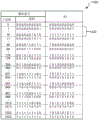
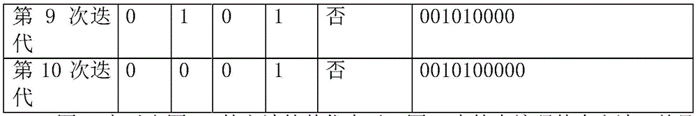
In various examples, one or more padding bits may be used when encoding the reference value and no padding bits may be used when encoding the difference value. This is because, as shown in fig. 10B, the probability distribution of the shifted reference values is not distributed as closely around 0 as the difference. Referring to the previous example, where the data word comprises three 10-bit input values (K3, L10), there may be two padding bits (forming a 32-bit data word) and these two padding bits may be used to encode the reference value such that for the first and third input values the result code comprises 10 bits (N) 0=N210) and for a second input value, the result code comprises 12 bits (N)112) in the above example, the input values 485, 480, 461 are decorrelated (in block 902) to give 5, 992, 1005, and these are then symbol remapped (in block 202) to generate three probability indices: x is the number of0=10,x163 and x237. Then, a subset of the codes is identified (in block 402) by using the method of FIG. 5A, such that R0=1,R 12 and R 22 and the updated probability index is x0=9,x150 and x226 and then identifies (or generates) codes with assigned hamming weights using a LUT or the method of fig. 6A, which may be mapped to the codes (in block 204). The resulting codes are 1000000000, 010000100000 and 0010100000.
Although in this example, all of the padding bits (e.g., both of the available padding bits used to pad three 10-bit input values into a 32-bit data word) are used to encode only one of the input values in the data word, in other examples, the padding bits may be shared between two or more of the input values. For example, where three 8-bit input values are packed into a 32-bit data word, each input value may be mapped to a 10-bit code (N ═ 10) and there may be two unused pad bits, or alternatively, two input values may be mapped to a 10-bit code and one input value may be mapped to a 12-bit code, such that all pad bits are used.
In case the input values have a non-uniform probability distribution or the input values have a uniform random probability distribution, the above-described method may be used; however, for input values having a uniform random probability distribution, and where N ═ L, the above approach may not provide any significant benefit in reducing the power consumed in transmitting and/or storing data. However, variations of the above-described method may be used to reduce power consumed in transmitting and/or storing data, where one or more padding bits (i.e., where N > L) are present for data having a uniform probability distribution (e.g., for random data). In such an example, as shown in fig. 17, rather than mapping the input values based on separately determined probability distributions (as in block 104), L-bit input values are mapped to an N-bit code, where N > L (block 1702). As part of this mapping operation (in block 1702), instead of determining a separate probability index (e.g., in block 202), the L-bit input value itself is used as the probability index. Alternatively, in the rare case where a decorrelation operation is used (e.g., in block 902) and results in input values with a uniform random probability distribution, the L-bit values generated from the L-bit input values in the decorrelation operation are used as probability indices. In the method of FIG. 17, L-bit values are mapped to an N-bit code based on the L-bit input value itself, where N > L (in block 1702).
In a variation shown in FIG. 4 and described above, the subset of identification codes may first be based on the L-bit value (block 1704), and then one of the subset of identification codes (block 404). This may be done using a LUT (e.g., as described above, e.g., with reference to fig. 3) and/or using an iterative process (e.g., as described above with reference to fig. 6). As a result of the grouping and ordering of the N-bit codes based on their HW (as detailed above), the random input value data is mapped to the most power efficient subset of codes. Although fig. 17 does not show the optional pair of pre-processing and post-processing operations (blocks 802 and 804) of fig. 8A and 8B, these may also be used in situations where the input data values do not have a probability distribution (e.g., for substantially random input data).
As described above, in some examples (whether the data has a non-uniform probability distribution or is substantially random), multiple input values may be grouped into a data word. In such an example, the result codes (one for each input value) may be grouped (e.g., multiplexed) into output data words in any order, as the order does not affect the HW of the output words. For example, as in the example above, where the result codes are 1000000000, 010000100000, and 0010100000, the code generated by the reference value may be packed at the end of the data word because it uses an additional P padding bits, which may simplify multiplexing of the codes to form the output data word. The resulting output data word with hamming weight 5 is given by:
10000000000010100000010000100000
If the largest factor in saving power is minimizing the hamming weight of the word, the output data word may be sent over the external bus to, for example, an external memory or another external module, such as a display controller.
However, if the larger factor in saving power when transmitting on the external bus is to minimize the number of bit flips, the same method as described above may be used and additional post-processing operations may be implemented (block 1302), as shown in FIG. 13. The processing operation thereafter (in block 1302) involves an exclusive or operation, as described below. Although fig. 13 is a variation of the method of fig. 9, post-processing operations (of block 1302) may also be used with the method of fig. 17, and/or post-processing operations (of block 1302) may be used without any decorrelation (i.e., block 902 is omitted). Furthermore, this post-processing may be used in conjunction with the optimization in the methods of fig. 8A and 8B. Alternatively, the exclusive-or operation may not be performed as a post-processing operation (as in block 1302), but rather as part of the process of generating the code, as shown in fig. 6B. As shown in fig. 6B, when compared to the initial method shown in fig. 6A (and described above), all flipped previous bits are appended (block 606) instead of appending 1 (block 616), except for the first bit, and the previous (not flipped) bit is appended (block 618) instead of appending 0 (block 608).
In a post-processing operation (block 1302), the code may be viewed as a list of differences, and each bit (except the first bit) may be xored in turn with its previous neighbor, where previously may be in the left or right direction depending on how the data was sent. In the following example, the previous neighbor is to the left, and the code:
10000000000010100000010000100000
to:
11111111111100111111100000111111
however, if the code is transmitted in a B-bit bus (where B is the bus width), then each bit (except for each of the first B bits) is not xored with its previous neighbor, but is in turn xored with the position before bit B, and in this example, the code:
10000000000010100000010000100000
it can be transmitted via a four-bit bus (B ═ 4) as follows:
channel 0: 10010000(3 bit turnover)
Channel 1: 00000100(2 bit overturn)
And (3) a channel 2: 00010010 (4-position turnover)
And (3) passage: 00000000(0 bit overturn)
Is transformed into:
10001000100000100010011001000100
it can be transmitted over a four-bit bus as follows:
channel 0: 11100000(1 bit overturn)
Channel 1: 00000111(1 bit overturn)
And (3) a channel 2: 00011100(2 bit overturn)
And (3) passage: 00000000(0 bit overturn)
It can be seen that this post-processing reduces the total number of bit flips from 9 to 4.
If the code is transmitted on buses of different widths, i.e. there is no uniform bus size B, the value of B may be chosen as the highest common factor of all bus sizes. For example, if the previous code (10000000000010100000010000100000) was transmitted over both a 4-bit bus and an 8-bit bus, it is post-processed using B-4, and this post-processing reduces the total number of bit flips on the 4-bit bus (from 9 to 4) and maintains the initial number of bit flips on the 8-bit bus (8 in total).
No post-treatment is required:
channel 0: 1000(1 bit turnover)
Channel 1: 0000(0 bit overturn)
And (3) a channel 2: 0001(1 bit turnover)
And (3) passage: 0000(0 bit overturn)
And (4) passage: 0100(2 bit turnover)
Passage 5: 0010(2 bit turnover)
Passage 6: 0100(2 bit turnover)
The passage 7: 0000(0 bit overturn)
Adopting post-treatment:
channel 0: 1100(1 bit turnover)
Channel 1: 0001(1 bit turnover)
And (3) a channel 2: 0010(2 bit turnover)
And (3) passage: 0000(0 bit overturn)
And (4) passage: 1000(1 bit turnover)
Passage 5: 0011(1 bit turnover)
Passage 6: 0110(2 bit turnover)
The passage 7: 0000(0 bit overturn)
It will be appreciated that this 32-bit example is quite short (in terms of number of bits per channel) and that for a larger number of bits more representative of a practical implementation, there will typically be a reduction in the number of bit flips on the 8-bit bus as well as the 4-bit bus.
In a further optional post-processing operation (in block 1302), if data is being streamed and access to previous B bits is available at both the encoding point and the decoding point, further power savings may be achieved by xoring each of the first B bits with its previous bit in the bitstream, and this may improve efficiency by a factor of M/(M-B), where M is the number of bits in the data word (e.g., M32). In this example, at least the final exclusive-or stage is inverted prior to storing the encoded data; unless the data is to be subsequently read out in the same order as written, for example when streamed.
As shown in FIG. 13, the post-processing operation of block 1302 may be used in conjunction with the decorrelation pre-processing operation of block 902, or may be used independently of the decorrelation operation.
In addition to the post-processing operations (block 1302) in fig. 13, many of the methods described above are described as operating so as to minimize (or at least reduce) the hamming weights (i.e., the number of 1 s) in the output code. In these cases, it can be said that the system has a target value of 0 for the hamming weight of the output code. However, there may be implementations where transmitting or storing is more power efficient than transmitting or storing 0, for example, due to asymmetries inherent in certain silicon processes. In these cases, it can be said that the system has a target value of the hamming weight of the output code, which is the maximum (and depends on the length of the code). The same method can be used when targeting the maximum hamming weight, with one additional operation being to flip all bits of the output code at the end of the method. Alternatively, the above method may be modified to replace the reference to 0 with the reference to 1, and vice versa (in blocks 606 and 608 of fig. 6A, in block 2202 of fig. 22, in blocks 2302 and 2307 of fig. 23, and in block 2402 of fig. 24). When a 1 is maximized instead of a 0, the pre-processing and/or post-processing operations described above with reference to fig. 8A, 8B, and 9 (e.g., in blocks 802, 804, and 902) may still be used. However, if a similar change is applied to the post-processing operation 1302 (or its equivalent as shown in fig. 6B), this will instead result in maximizing (rather than minimizing) the bit flip, and thus this may only be achieved if this is the desired result.
In some implementation scenarios, the system may benefit from maximizing 1 in some cases and 0 in other cases. To accomplish this, a flag (e.g., a single bit) may be provided that switches operation between the variant of the method that maximizes 1 and the variant of the method that maximizes 0.
As described above, in the mapping operation (in block 204), the probability index (and thus the input value) may be mapped to one of a set of predefined codes based on the number of 1's present in the predefined code or based on the number of multiple bit flips present in the predefined code. The above examples (except for fig. 6B and block 1302) all refer to the first of these options (i.e., based on the number of 1's); however, the mapping operation described above (including the case where there is a uniform probability distribution as in fig. 17) may also be used, where the mapping is performed based on the number of bit flips present in a predefined code (i.e., based on the number of transitions between 0 and 1 or between 1 and 0 in two consecutive bits within the code). This will result in a re-grouping of the codes into subsets, and thus also a reordering of the codes, e.g. compared to the LUT 300 of fig. 3. However, the regrouping of the codes now depends on whether the codes are streamed or not. If a code is being streamed, the previous neighbor can be used for exclusive-or, and each code starting with one (either left or right depending on the direction of the stream) indicates an implicit bit flip. An example LUT 1420 is shown in fig. 14A and the implicit bit flip can be seen from a second subset, subset 1422, which contains codes with one bit flip, including code 1111111111. If the code is not streamed, the previous neighbor is not available for exclusive-or, and an example LUT 1400 is shown in fig. 14B.
As shown in fig. 14B, the set or subset of 10-bit codes is subdivided into a plurality of subsets 1401-1410, each subset comprising two or more codes containing the same number of flips, e.g. the first subset 1401 comprises two codes without flips, the second subset 1402 comprises 18 codes with one flip, etc. Within each subset, codes with the same number of flips may be ordered in any manner, and in the example shown, they are ordered lexicographically. As shown in fig. 14B, although in very few cases the 10-bit binary version of the probability index matches the 10-bit code, in most cases the two are different.
In case the amount of flipping is used instead of HW, the binomial coefficients may be iteratively subtracted from the probability index x, for example Where N is the number of bits in the code, and initially r is 0. Fig. 15A shows an equivalent scheme to fig. 5A, where the hamming weight R is replaced by the number of flips F. As shown in fig. 15A, the probability index x is initially compared to twice the binomial coefficient where r is 0, which is equal to two (independent of the value of N) (block 1502) -as shown in fig. 15A, the binomial coefficient using the number of flips is
  Rather than that of
 Because there are N bit positions in an N-bit code, there are only N-1 points between bits where toggling can occur (unless xor across adjacent codes occurs, e.g., in streaming, in which case the previous method of fig. 6B is used, block 1302 or fig. 14A), but the (smaller) binomial coefficient is multiplied by two because there are two options for the value of the initial bit: 1 or 0 and then all other bits are determined by the number of bit flips and the location of those bit flips. If the probability index is strictly less than two (yes in block 1502), i.e., it is 0 or 1, then the
 first subset 1401 with a number of flips F of 0 is selected (block 1504). Otherwise, the value of twice the binomial coefficient is subtracted from the probability index (i.e., 2 in this first iteration) and the value of r is added to 1 (block 1506). In a subsequent iteration, the updated probability index x from the previous iteration is compared (in block 1502) to the current values of two times the binomial coefficient and r, and if the updated probability index x is strictly less than twoTwice the polynomial coefficient ("yes" in block 1502), a subset is selected where the number of flips is equal to the current value of r, i.e., where F equals r (block 1504). However, if the updated probability index x is not strictly less than twice the binomial coefficient ("no" in block 1502), then the value of twice the binomial coefficient (with the current value of r) is subtracted from the updated probability index and the value of r is incremented by 1 (block 1506). The values of the binomial coefficients (or twice those binomial coefficients) used in selecting the subsets (in blocks 1502 and 1506) may be calculated or may be pre-generated and obtained from the LUT (e.g., in a similar manner as described above with reference to fig. 5A). Further, in a manner similar to the modification from the method shown in fig. 5A to the method shown in fig. 5B, the method of fig. 15A may be modified to use an accumulated version of the binomial coefficients, and/or the values in the LUT may be accumulated versions to reduce throughput, latency, and power (as described above with reference to fig. 5B), as shown in fig. 15B. As shown in fig. 15B, by using the accumulated values (in the comparison of block 1512), the update step in the loop (block 1516) includes only an increment of the r value (rather than also updating the value of the probability index as in block 1506 of fig. 15A), and there is a single subtraction operation (block 1514) that computes the final, updated probability index x value. This subtraction operation (in block 1514) subtracts from the initial probability index the accumulated value that is readable from the LUT  To produce a final updated version of the probability index in a single step. In another variation, instead of storing binomial coefficients, only binomial coefficients may be stored in the LUT (i.e., not multiplied by two), and the multiplication by two may be performed dynamically, i.e., by shifting the bit by one bit position.
Once the subset is identified (in block 402), for example using one of the methods described above, the code may be selected (in block 404) from the identified subset using information determined as part of the identification of the subset, as previously described. The codes within each subset may be stored in the LUT and selected based on the final updated value of the probability index x, or alternatively, the codes may be generated one bit at a time in an iterative process using the final updated value of the probability index x. As shown in fig. 22. As shown in fig. 22, the iterative method uses two iteration values N and r, and initially N-1 (where N is the bit length of the code, as described above) and r-F (where F is the number of flips in the identified subset, as described above), and, after the preprocessing stage (block 2202-2206), N is decremented by 1 (block 2208) so that there are exactly N-1 iterations (N-2, N-3,. once, 1, 0 each).
In the pre-processing stage of the method of FIG. 22, zeros are appended to the code (block 2202) and if the final updated value of the probability index x is greater than or equal to the binomial coefficient (YES in box 2204), then set flag and by setting x equal to
 To reduce the value of the probability index (block 2206). In each subsequent iteration, n is decremented by 1 (block 2208) and the updated probability index x is compared to the binomial coefficient having the current values of n and r
 A comparison is made (block 2210). If the updated probability index x is greater than or equal to the binomial coefficient
 (YES in block 2210), an inverted version of the previous bit (i.e., the bit most recently appended to the code) is appended to the code, and the binomial coefficient is subtracted from the probability index x
 And r is decremented by 1 (block 2212). However, if the updated probability index x is not greater than or equal to the binomial coefficient
 (no in block 2210), the previous bit is appended to the code and the values of x and r are unchanged (block 2214). When n is equal to 0 (frame)2216) and then there is a post-processing stage, the iterative loop stops. In the post-processing phase, if the flag is set in the pre-processing phase ("yes" in block 2218), all bits in the code are flipped (block 2220). If the flag is not set ("NO" of block 2218), the bits in the code are not flipped. The flag may be encoded as a direct signal between
 blocks 2206 and 2218, or it may be stored as extra bits next to the output code, which are discarded during post-processing.
Fig. 23 shows another iterative method of generating a code that is a variation of the code shown in fig. 22 and described above. Unlike the method of fig. 22, the method of fig. 23 avoids the need for post-processing operations and does not involve the storage of flags (either as system state or as extra bits next to each code). Thus, the method of fig. 23 is more efficient than the method of fig. 22. As shown in fig. 23, a 1 or 0 is initially appended (in block 2307 or 2302) depending on the result of the first comparison (in block 2204), and by setting the initial bits of the code in this manner, it is not necessary to flip all bits in the code according to the stored flag value.
In many of the examples described above, the input values all have the same length, i.e., L bits, and the length of the output code, i.e., N bits. As described above, in various examples, the input values and/or output values may vary in length, and this may depend on the manner in which the input values are generated. In one example, the input values may be generated using huffman coding, and in a particular example using alphabetic symbols and their associated probabilities, these may be encoded by starting with a null output binary string assigned to the leaf nodes for each input character. These leaf nodes are used as the basis for building a binary tree. The data is processed by finding at each step the two unprocessed nodes with the smallest probability and creating a new node, the probability of which is given by the sum of the first two nodes. The output binary string of the first/second previous node (and all nodes below it in the hierarchy) has 0/1 pushed ahead of its output code, with nodes with higher probabilities assigned 0 and nodes with lower probabilities assigned 1 (by assigning 1 and 0 in this manner instead of arbitrarily, resulting in a reduction of up to 9% of the average hamming weight in the following example). The two previous nodes are then considered processed and are then ignored when selecting a node. This is iteratively repeated until only a single unprocessed node (referred to as the root node with probability 1) remains. The process builds a binary tree in which each newly created node is connected to two previous nodes that generated it, and in which the input characters further downstream in the hierarchy (corresponding to leaf nodes) have longer output binary codes assigned to them.
The resulting binary code has an arbitrary number of bit lengths, so it may be desirable to pad the code to multiples of 4 bits in order to reduce the multiplexing (i.e., multiplexing) logic in the hardware, and so in this example, it is desirable to pad each encoded input character to 4, 8, or 12 bits long. Since naturally filling the huffman code with 0 does not provide a gain, e.g. a reduction of HW, the encoded input characters can be used as input to the method described herein to map them to more power efficient output codes of length 4, 8 or 12 bits.
The huffman-coded input characters form the input values for the encoding method described herein and the probability data used in the huffman coding may no longer be available for the probability ordering operation (in block 202). Although in this case the ordering given by the initial probability data is not available, it is implicitly stored in the huffman-coded input values from the length and value of the code, and can therefore be deduced from them using an ordering algorithm, for example by performing repeated pairwise comparisons of input values (e.g. bubbling or fast ordering) to place the input values from highest to lowest by probability: if two input values have different lengths, the shorter one has a higher probability, and if the two values have the same length, the smallest has a higher probability in a dictionary manner. For the length L aAnd LbWith unknown probability paAnd pbWrite as:

by treating two codes of equal length as LaBit integers to give the final inequality. This classification and subsequent binary generation (described below) may be performed offline (rather than on-the-fly) and used to generate the LUT. At run-time, the code may be identified by indexing in the LUT, and at run-time this is more efficient in terms of processing and latency, especially for large data sets.
As described above, after the input values are sorted and thus implicitly assigned probability indices, they are mapped to one of a set of predefined codes (in block 204), where in this example the length of the output code for a given input value is a length of 4 bits (i.e., 4, 8, or 12 bits) with the input value rounded to the next multiple. Thus, the output code meets the requirements of nibble stride, but also retains most of the benefits of variable length entropy coding.
In order for the code to be prefix-free (i.e., if concatenated, no separate length storage is required), the first 4/8 bits of the 8/12 bit code must be different from any of the 4/8 bit codes themselves. Thus, the 8-bit code words may be set to all start with the same prefix of 1010, which continues from the least probable 4-bit code word of "r" of 1001, and all 12-bit code words may be set to start with 10101101, which continues from the least probable 8-bit code word of "k" of 10101011.
For this example, the result of the character ordering according to its probability maps as follows:
| letters | Input value | Code | Letters | Input | Code |
| e | |||||
| 011 | 0000 | m | 1100,0 | 1010,1000 | |
| |
111 | 0001 | w | 1100,1 | 1010,0011 |
| a | 0001 | 0010 | f | 1101,0 | 1010,0101 |
| o | 0010 | 0100 | g | 0011,00 | 1010,0110 |
| i | 0100 | 1000 | |
0011,01 | 1010,1001 |
| n | 0101 | 0011 | |
0011,10 | 1010,1010 |
| s | 1000 | 0101 | |
0011,11 | 1010,1100 |
| |
1001 | 0110 | |
1101,11 | 1010,0111 |
| r | 1010 | 1001 | |
1101,100 | 1010,1011 |
| |
0000,0 | 1010,0000 | |
1101,1010,0 | 1010,1101,0000 |
| |
0000,1 | 1010,0001 | x | 1101,1010,1 | 1010,1101,0001 |
| |
1011,0 | 1010,0010 | |
1101,1011,0 | 1010,1101,0010 |
| |
1011,1 | 1010,0100 | |
1101,1011,1 | 1010,1101,0100 |
From this it can be seen that although in some cases the input values and the output codes may be the same, in most cases they are different, and that the average relative HW (i.e. where "average" represents the relative HW solution for all output codes weighted by their associated probability, and "relative HW" refers to HW as the proportion of code length, which is a better measure for variable length codes than simply HW) is reduced by more than 15% in the above example compared to filling only the initial huffman code, thus providing a corresponding power saving.
Another example method of power-efficient encoding of data may be described with reference to fig. 16. Although the method of fig. 16 may be used as a post-processing operation of the above-described method, in most examples, the method is used independently. The method of fig. 16 is simpler to implement than the above-described methods, but the earlier methods provide improved performance (e.g., greater improvement in power consumption).
The method of fig. 16 may be used to reduce the hamming weight of data that will be transmitted anywhere there are one or more unused padding bits on the external bus. By reducing the HW of the transferred data, the power efficiency of the data transfer is improved independently of the width of the bus sending the data (which may be an internal or external bus), e.g. if the bus width is known or unknown. The method provides an improvement in power efficiency even if the input values have a uniform random probability distribution and can be used, for example, for the above-described types of data or other types of data such as pointer data (e.g., where they are aligned to a particular level of granularity). Unlike known techniques, the method of FIG. 16 does not require any knowledge of the bus (or memory line) width or any control over the order of data writes/reads (e.g., where there is a cache or combination of writes performed by hardware).
Although the following description of the method of fig. 16 refers to reducing the hamming weight of data based on determining how many (or what proportion) of the bits are 1, more generally, the method may be based on determining how many (or what proportion) of the bits have a predefined value (e.g., set to 1 or 0 here) such that the hamming weight is reduced (the predefined value is set to 1 here) or increased (the predefined value is set to 1 here). The selection of the predetermined value may depend on the particular architecture and hardware used.
In the case where there is one unused pad bit, the method of fig. 16 may be applied to all other bits in the data word. In other examples, other bits in the data word may be subdivided into portions, where one of the portions corresponds to unused padding bits, and the method of fig. 16 may be applied to that portion and not to the other portions. Where there is more than one unused pad bit, other bits in the data word may be subdivided into portions, with each portion or a subset of the portions corresponding to one of the unused pad bits, and the method of fig. 16 may be applied to each portion having corresponding unused pad bits independently of the other portions. In various examples in which the data word is subdivided into a plurality of portions, the portion sizes may be selected such that each portion has an even bit length, and in various examples, different portions may have different bit lengths.
As shown in fig. 16, the method includes determining whether a bit sequence (which, as described above, may include some or all of the bits in a data word other than the corresponding unused pad bits) includes more 1's than 0's (block 1602), and if 1's are less than 0's, or have the same number of 1's and 0's (no in block 1602), setting the corresponding pad bits to a value (e.g., 0) indicating that the bit sequence is not flipped (block 1604). In contrast, if there are more 1 s in the bit sequence than 0 (yes in block 1602), the corresponding pad bits are set to a value (e.g., 1) indicating that the bit sequence has been flipped (block 1606), and all bits in the bit sequence are flipped, i.e., inverted (block 1608). This therefore reduces the hamming weight of the bit sequence transmitted on the external bus and caps the maximum hamming weight to the cell (N/2), where N is the number of bits in the bit sequence that includes the padding bits.
While this method of FIG. 16 may yield less benefit only if the input values rarely have high Hamming weights (e.g., HW >. N/2.), the method provides greater benefit in examples where input values often have high Hamming weights. For example, if the input values represent unsigned integers, the value with high HW will be mainly the maximum value in the set. For example, if the input values represent signed integers, the values with high HW will be mostly least negative. The method provides improved efficiency for input values with uniform random probability, but the improvement is less than if the distribution is skewed to higher HW, since each input value has equal probability.
By using the method of fig. 16 independently of the other methods described herein, HW of video data may be reduced by up to about 20%, depending on the nature of the video data. In contrast, by using other methods described herein (e.g., the method of fig. 1 with various optional pre-processing and post-processing stages), the HW of the video data can be reduced by more than 50%, and for some types of video data can be reduced by as much as 80%.
Although not shown in fig. 16, in various examples, the decorrelation operation (block 902) described above may be used as a pre-processing step of the method of fig. 16. This provides an additional improvement over the benefits obtained using the method, as the bit flipping of fig. 16 makes the greatest improvement in values with high HW (e.g., small negative values).
Although the above method has been described as improving data transmission efficiency on the external bus and data storage efficiency in the external memory, power efficiency may be improved in the case where data is transmitted through the internal bus and/or stored in the local cache. In such examples, the methods described herein may be implemented at the end of a processing operation that produces input values, such as at the end of a tile that processes graphics data.
The above method relates to encoding of data values. Prior to using the encoded data values, and in some examples, prior to storing the encoded data values, a decoding method may be used to recover the original input values. Decoding encoded data values generated using any of the methods described herein may be performed by reversing each stage of the method and performing the stages in reverse order.
Referring to the encoding method of fig. 2, the corresponding decoding method includes mapping each code to a probability index (i.e., in an operation opposite to the probability index of block 204), and then determining an input value corresponding to each probability index (i.e., in an operation opposite to the probability index of block 202). The mapping from the code to the probability index (in the inverse of block 204) uses the same binomial coefficients (and thus may use the same LUT) as used in the code generation.
The mapping methods described with reference to fig. 5A, 5B, 6A and 6B may map the codes back to the probability indices by performing these methods in reverse as shown in fig. 24 to determine the position of the codes within their respective subsets. The method iterates using three parameters n, x and r, which may all be initially set to 0. The method checks the LSB of the code and if it is one (YES in block 2402), the values of x and r are updated (blocks 2404A or 2404B, where the implementation of block 2404B is more efficient because it saves on addition operations Do so). Regardless of the value of the LSB, the LSB is then removed from the code (block 2406), the value of n is incremented (block 2407), and the method continues to check for a new LSB in each subsequent iteration until there are no bits remaining in the code (no in block 2408). At this point (i.e., after "no" in block 2408), the final value of R is set to the hamming weight R (in block 2410), and the final value of x may be calculated in block 2412 as Where the values of the cumulative binomial coefficients can be read from the LUT. The final value of x is then output (as calculated in block 2412) (block 2414).
Although the method of fig. 24 involves removing the LSBs in each iteration of the loop (in block 2406), in other examples, the method may step through the binary code from LSB to MSB. In such an example, the decision box at the end of the loop (box 2408) may be expressed as "N < N? And this variation can also be used in the case of removing the LSB (as shown in fig. 24).
In the method of fig. 24, incrementing of x (in block 2404A or 2404B) within the loop corresponds to the reverse operation of fig. 6A, i.e., finding an output code within the subset corresponding to a given hamming weight R, adding the final binomial coefficient to x (in block 2412) after the loop corresponds to cancelling the operation of fig. 5A or 5B, i.e., finding the subset given hamming weight R into which the initial x falls and modifying it accordingly to the relative index.
Referring to the table shown in fig. 7, which may be used to map probability indices to codes and codes to probability indices, 1's and 0's in the codes describe paths through the table (left to right) where each binomial coefficient arriving after a bit value of one is accumulated to the current total (which is initially 0). Starting from the LSBs of the code word, each LSB corresponds to a step down and to the right, and the binomial coefficients reached by this step are added to the current sum. Each 0 in the code corresponds to only one step to the right, and in this case the current total is not modified. Since there are N bits and R1 s in the code, the process is in place And terminates. This therefore corresponds to the block within the loop of fig. 24. Adding the final sum to the cumulative binomial coefficient
 To produce a probability index for the codeword and this corresponds to the block following the loop of fig. 24.
After the probability index is generated, it is mapped back to the input value. Where such probability ordering (in block 202) uses symbol remapping, the input value may be identified by canceling the symbol remapping by: the LSB is removed, the remaining bits are shifted to the right by one bit position (which involves adding a 0 as the MSB), and then all L bits (i.e., the bits remaining after the LSB is removed plus the newly added MSB) are exclusive-ored with the removed LSB. In the case of modified sign remapping for floating point inputs, the operation is reversed by only moving the LSB to the MSB. Thus, both the probability index and the input value include L bits. In those examples where decorrelation is performed (in block 902) when the input values are encoded, the values generated by inverse sign remapping are the decorrelated input values, and thus the method further comprises inverting the decorrelation, e.g., by shifting the reference values by the median value and then shifting the other values by the modified reference values or generally canceling the initial linear or affine transformation. However, in the case where decorrelation is not performed while encoding an input value, a value generated by the sign inverse remapping is an actual input value, and decoding is completed.
In the case where the probability index is generated from the input value by referring to the LUT, the input value is also decoded from the probability index by referring back to the LUT.
Referring to the encoding method of fig. 16, when used independently of any other method described herein, the corresponding decoding method comprises: for each bit segment (where there may be one or more segments in the data word), the value of the corresponding padding bit is read, and if the padding bit indicates that the segment is flipped during the encoding process, all bits in the segment are flipped and the padding bit is reset to its default value, and if the padding bit indicates that the segment is not flipped during the encoding process, the bits in the segment are left unchanged and the padding bit is reset to its default value.
Fig. 3, 14A and 14B illustrate example LUTs, and it will be appreciated that in other examples, the entries within each subset (e.g., each HW subset of fig. 3 and 14A) may be rearranged to reduce the number of gates required to encode the LUT.
Fig. 18 and 19 illustrate two example hardware implementation scenarios 1800, 1900 in which the methods described herein may be implemented. In a first example, as shown in fig. 18, two computing entities 1802, 1804 are shown and may be peripherals, processors or memory. The first computing entity 1802 in fig. 18 includes an extraction/output hardware block 1812 arranged to output data values to an encoding hardware block 1822 arranged to perform one of the encoding methods described herein. The resulting encoded data is carried on the bus 1806 and decoded at the second computing entity 1804. The second computing entity includes a decoding hardware block 1814 arranged to perform the inverse of the encoding method implemented by the first computing entity 1802, and the decoded data items are then input to an input/storage hardware block 1824.
In various examples, the encoding hardware block 1822 includes an input 1826, an output 1828, and hardware logic 1830, which may be referred to as mapping hardware logic. The input 1826 is configured to receive a plurality of input values, the mapping hardware logic 1830 is arranged to map each input value to one of a set of predefined codes based on a probability distribution of the input values and a characteristic of the code, wherein the characteristic of the code comprises a hamming weight of the code or a number of bit flips within the code, and the output 1828 is arranged to output the code corresponding to the received input value. In such an example, the decode hardware block 1814 includes an input 1832, an output 1834, and hardware logic 1836, which may be referred to as mapping hardware logic. The input 1832 is configured to receive a plurality of input codes, the mapping hardware logic 1836 is arranged to map each input code to one of a set of predefined decoded values based on a probability distribution of the decoded values and a characteristic of the code, wherein the characteristic of the code comprises a hamming weight of the code or a number of bit flips within the code, and the output 1834 is arranged to output a decoded value corresponding to the received input code.
In other examples, the encoding hardware block 1822 still includes inputs 1826 and outputs 1828 and hardware logic 1830. As described above, input 1826 is configured to receive a plurality of input values, however, in these examples, each input word includes one or more input values and one or more padding bits. In these examples, the hardware logic 1830 operates differently and is instead arranged to determine whether more than half of the bits in a portion of the input word are 1's and, in response to determining that more than half of the bits in a portion of the input word are 1's, generate an output word by inverting all of the bits in the portion and setting the padding bits to a value indicative of the inversion. In these examples, output 1828 is arranged to output words. In these examples, the decode hardware block 1814 includes an input 1832, an output 1834, and hardware logic 1836. Input 1832 is configured to receive a plurality of input words, where each input word includes a segment of one or more bits and a fill bit corresponding to each segment. The hardware logic 1836 is arranged to, for each portion of the input word: reading and analyzing the value of the corresponding padding bit; in response to determining that the padding bits indicate that the segment flipped during the encoding process, flipping all bits in the segment and resetting the padding bits to their default values; and in response to determining that the padding bits indicate that the segment has not flipped during the encoding process, leaving the bits in the segment unchanged and resetting the padding bits to their default values. The output 1834 is arranged to output the resulting bits as a decoded word.
In the second example shown in fig. 19, there are three computing entities 1802, 1804, 1908. The first two of these are as described above with reference to fig. 18, and the third entity 1908 is a memory. In this second example, unlike the first example, the encoded data is carried on the bus 1806 and stored in the memory 1908, and the data is not decoded until it is needed by the second computing entity 1804. In this second example, it is understood that the first entity 1802 and the second computing entity 1804 may be the same computing entity.
It should be understood that the computing entities 1802, 1804 shown in fig. 18 and 19 may include many additional elements not shown in fig. 18 and 19, for example, the encoding and decoding blocks may be pre-processed and post-processed by others to encode/compress and decode/decompress blocks, respectively, to further modify the encoding to improve other properties independent of the reduction in HW.
There are many example use cases for the methods described herein. For example, when pixel data is written from the buffer to the screen, and in this example, the data is typically correlated and filled. The methods described herein may also be used as part of a video system after decoding normal variable length compression before being passed to a screen or other device. The methods described herein may be substituted for or coupled with any compression/decompression pipeline (as the data will typically have an associated distribution). This improves the system from just bandwidth savings to power savings. Compression/decompression pipelines are widely used because compression is typically applied to images/video/textures/audio, etc. The method may also be used for other types of related data or data that is padded to a power of 2 bits (e.g., a user-defined structure that does not fill a power of two bytes).
Fig. 12 described above illustrates the effect of additional padding bits on the first method described herein (e.g., the methods of fig. 1-16). As shown in fig. 12, the method continues to achieve up to a total of 2LThe benefit of L-1 padding bits, although each additional padding bit has less and less effect. In contrast, the second approach (as described above with reference to fig. 16) does not benefit from having more than L/2 pad bits (as no benefit is gained by using flag bits on input values less than 2 bits). Some example maximum numbers of padding bits for both methods are given below for various values of L:

the efficiencies that can be achieved using the above-described methods (in addition to the method of fig. 16) can be illustrated as follows.
Let i be as large as 2N={0,1,...2N-1 is the coded outputValue of
Let p bei∈[0,1]Is a probability of i such that
Letting H: 2N→N, Is a function of hamming weight
The average hamming weight W is given by

Let HnIs a code set of Hamming weights N ∈ {0, 1.. N }
Let p benIs the sum of the probabilities of the input codes HnThen


It can be shown that W is precisely minimized when the following criteria are met:

Assuming that the codes have been assigned to probabilities such that they satisfy the above criterion (, the first choice is by any two Hamming weight bucket indices i and j in {0, 1, … N }, wlog j ≦ k and the choice is by any two indices i from these buckets j∈HjAnd ik∈HkAre formed respectively with probabilities And
And this gives:
k=j+l,l∈N0

probability of exchange ijAnd ikGiven a new average hamming weight W', which is greater than or equal to W as follows:

the condition that W' ≧ W is therefore equal is if and only if k ═ j (i.e., both code values already have the same hamming weight) or (i.e., the two encoded values have the same probability). In either case, the transposed code also satisfies (#).
Thus, it has been shown that the criteria given by (, a) determine the set of H.W minimum encodings for a given probability distribution, and are all local minima. By considering any other codes with probabilities that are not ordered in this way, the same logic makes clear that there is a transposition of a pair of probabilities that reduces the average hamming weight by some non-0 amount-so they are in fact all global minima.
If the second method described above (i.e., the bit flipping method of fig. 16) is used as an alternative to reducing the average hamming weight of the encoded value (i.e., if more than half of the bits are set, all the bits are flipped, and one of the padding bits is marked to identify this), then a particular type of data is required to be valid since the encoded value is modified in a fixed manner regardless of the probability distribution of the data. This is data with a probability distribution skewed to codes with a small number of 1's or a small number of 0's, and conversely, the worst kind of data is those data with a probability skewed to codes with a similar number of 0's and 1's. Signed data fits well to an efficient type of distribution, so decorrelated data should also benefit the method.
This can be explicitly shown by the following logic, where N ═ L +1, i.e., a single pad bit is used for the flag, and N and L are the length of the code with and without the pad bit flag, respectively:

this is optimal in the following cases:


FIG. 20 illustrates a computer system 2000 in which the methods described herein may be implemented. The computer system includes a CPU 2002 (which may correspond to CPU 1800 shown in fig. 18 and described above) and a GPU 2004 (which may correspond to GPU1900 shown in fig. 19 and described above). In addition, the computer system 2000 includes a memory 2006 and other devices 2014, such as a display 2016, speakers 2018, and a camera 2020. Processing block 910 (corresponding to processing block 110) is implemented on GPU 904. The components of the computer system communicate with each other over a communication bus 2024.
The processor of fig. 18 and 19 and the computer system of fig. 20 are shown as including a number of functional blocks. This is merely illustrative and is not intended to define a strict division between different logical elements of such an entity. Each of the functional blocks may be provided in any suitable manner.
The processors described herein may be embodied in hardware on an integrated circuit. The processor described herein may be configured to perform any of the methods described herein. Generally, any of the functions, methods, techniques, or components described above can be implemented in software, firmware, hardware (e.g., fixed logic circuitry), or any combination thereof. The terms "module," "function," "component," "element," "unit," "block," and "logic" may be used herein to generally represent software, firmware, hardware, or any combination thereof. In the case of a software implementation, the module, functionality, component, element, unit, block, or logic represents program code that performs specified tasks when executed on a processor. The algorithms and methods described herein may be executed by one or more processors executing code that causes the processors to perform the algorithms/methods. Examples of a computer-readable storage medium include Random Access Memory (RAM), Read Only Memory (ROM), optical disks, flash memory, hard disk memory, and other memory devices that may use magnetic, optical, and other techniques to store instructions or other data and that may be accessed by a machine.
The terms computer program code and computer readable instructions as used herein refer to any kind of executable code for execution by a processor, including code expressed in a machine language, an interpreted language, or a scripting language. Executable code includes binary code, machine code, bytecode, code defining an integrated circuit (e.g., a hardware description language or netlist), and code expressed in programming language code such as C, Java or OpenCL. The executable code may be, for example, any kind of software, firmware, script, module or library that, when executed, processed, interpreted, compiled, run-time appropriately in a virtual machine or other software environment, causes the processor of the computer system supporting the executable code to perform the tasks specified by the code.
A processor, computer, or computer system may be any kind of device, machine, or special purpose circuit, or collection or portion thereof, that has processing capabilities such that instructions may be executed. The processor may be any kind of general or special purpose processor such as a CPU, GPU, system on a chip, state machine, media processor, Application Specific Integrated Circuit (ASIC), programmable logic array, Field Programmable Gate Array (FPGA), Physical Processing Unit (PPU), Radio Processing Unit (RPU), Digital Signal Processor (DSP), general purpose processor (e.g., general purpose GPU), microprocessor, any processing unit intended to accelerate tasks other than CPU, etc. A computer or computer system may include one or more processors. Those skilled in the art will recognize that such processing capabilities are incorporated into many different devices, and thus the term "computer" includes set-top boxes, media players, digital radios, PCs, servers, mobile phones, personal digital assistants, and many other devices.
The present invention is also intended to encompass software defining the configuration of hardware as described herein, such as Hardware Description Language (HDL) software, for designing integrated circuits or for configuring programmable chips to perform desired functions. That is, a computer-readable storage medium may be provided having computer-readable program code encoded thereon in the form of an integrated circuit definition dataset that, when processed (i.e., executed) in an integrated circuit manufacturing system, configures the system to manufacture a processor configured to perform any of the methods described herein, or a processing system including any of the devices described herein. The integrated circuit definition data set may be, for example, an integrated circuit description.
Accordingly, a method of manufacturing a processor or other hardware logic configured to perform one of the methods as described herein at an integrated circuit manufacturing system may be provided. Furthermore, an integrated circuit definition dataset may be provided, which when processed in an integrated circuit manufacturing system, causes a method of manufacturing such a processor or hardware logic to be performed. In various examples, the encoding method may be implemented in software/firmware (e.g., using block 202 in fig. 5A or 5B and in fig. 6A or 6B plus an iterative process). In other examples, the method may be implemented as a fixed function hardware unit and/or a set of connected arithmetic units that use a data structure (e.g., a set of gates or an array of table entries) to encode part or all of the mapping (as a LUT) to perform the method of fig. 5A or 5B and fig. 6A or 6B.
The integrated circuit definition data set may be in the form of computer code, e.g., as a netlist, code for configuring a programmable chip, as a hardware description language for defining integrated circuits at any level, including as Register Transfer Level (RTL) code, as a high-level circuit representation, e.g., Verilog or VHDL, and as a low-level circuit representation, e.g., oasis (rtm) and GDSII. A higher-level representation (e.g., RTL) of an integrated circuit that is logically defined may be processed at a computer system configured to generate fabrication definitions for the integrated circuit in the context of a software environment that includes definitions of circuit elements and rules for combining those elements to generate the fabrication definitions for the integrated circuit defined by the representation. As is often the case with software executed at a computer system to define a machine, one or more intermediate user steps (e.g., providing commands, variables, etc.) may be required to configure the computer system to generate a manufacturing definition for an integrated circuit to execute code that defines the integrated circuit to generate the manufacturing definition for the integrated circuit.
An example of processing an integrated circuit definition data set at an integrated circuit manufacturing system in order to configure the system to manufacture a processor or other hardware logic configured to perform one of the methods as described herein will now be described with reference to fig. 21.
Fig. 21 illustrates an example of an Integrated Circuit (IC) manufacturing system 2102 configured to manufacture a processor or other hardware logic configured to perform one of the methods as described herein. In particular, IC manufacturing system 2102 includes a layout processing system 2104 and an integrated circuit generation system 2106. The IC manufacturing system 2102 is configured to receive an IC definition dataset (e.g., defining the processors 1800, 1900 as described in any example herein), process the IC definition dataset, and generate an IC from the IC definition dataset (e.g., embodying hardware logic arranged to perform a method as described in any example herein). The processing of the IC definition dataset configures the IC manufacturing system 2102 to manufacture an integrated circuit embodying hardware logic arranged to perform a method as described in any example herein.
The layout processing system 2104 is configured to receive and process an IC definition data set to determine a circuit layout. Methods of determining circuit layouts from IC definition data sets are known in the art AND may, for example, involve synthesizing RTL codes to determine a gate-level representation of the circuit to be generated, for example in terms of logic components (e.g., NAND, NOR, AND, OR, MUX, AND FLIP-flow components). By determining the location information of the logic components, the circuit layout can be determined from the gate level representation of the circuit. This may be done automatically or with user involvement to optimize the circuit layout. When the layout processing system 2104 has determined the circuit layout, it can output a circuit layout definition to the IC generation system 2106. The circuit layout definition may be, for example, a circuit layout description.
As is known in the art, the IC generation system 2106 generates ICs from circuit layout definitions. For example, the IC generation system 2106 may enable a semiconductor device manufacturing process that generates ICs, which may involve a multi-step sequence of photolithography and chemical processing steps during which electronic circuits are gradually formed on a wafer made of semiconductor material. The circuit layout definition may be in the form of a mask, which may be used in a lithographic process to generate an IC from the circuit definition. Alternatively, the circuit layout definition provided to the IC generation system 1006 may be in the form of a computer readable code that the IC generation system 1006 may use to form a suitable mask for generating the IC.
The different processes performed by the IC manufacturing system 2102 may all be performed at one location, for example, by a party. Alternatively, the IC manufacturing system 2102 may be a distributed system, such that some processes may be performed at different locations and by different parties. For example, some of the following stages may be performed at different locations and/or by different parties: (i) synthesizing an RTL code representing the IC definition data set to form a gate level representation of the circuit to be generated; (ii) generating a circuit layout based on the gate level representation; (iii) forming a mask according to the circuit layout; and (iv) using the mask to fabricate the integrated circuit.
In other examples, processing of the integrated circuit definition data set at the integrated circuit manufacturing system may configure the system to manufacture hardware logic arranged to perform the method as described herein without processing the IC definition data set in order to determine the circuit layout. For example, an integrated circuit definition dataset may define a configuration of a reconfigurable processor, such as an FPGA, and processing the dataset may configure the IC manufacturing system (e.g., by loading configuration data into the FPGA) to generate the reconfigurable processor with the defined configuration.
In some embodiments, the integrated circuit fabrication definition data set, when processed in an integrated circuit fabrication system, may cause the integrated circuit fabrication system to generate an apparatus as described herein. For example, a device as described herein may be manufactured by configuration of an integrated circuit manufacturing system in the manner described above with respect to fig. 21, via an integrated circuit manufacturing definition data set.
In some examples, the integrated circuit definition dataset may include software that runs on or in combination with hardware defined at the dataset. In the example shown in fig. 21, the IC generation system may be additionally configured by the integrated circuit definition dataset to load firmware onto the integrated circuit according to the program code defined in the integrated circuit definition dataset when the integrated circuit is manufactured, or to otherwise provide the integrated circuit with program code for use with the integrated circuit.
Those skilled in the art will realize that storage devices utilized to store program instructions may be distributed across a network. For example, a remote computer may store an example of the described process as software. A local or terminal computer may access the remote computer and download a part or all of the software to run the program. Alternatively, the local computer may download pieces of the software, as needed, or execute some software instructions at the local terminal and other software instructions at the remote computer (or computer network). Those skilled in the art will also realize that by utilizing conventional techniques known to those skilled in the art that all, or a portion of the software instructions may be carried out by a dedicated circuit, such as a DSP, programmable logic array, or the like.
The methods described herein may be performed by a computer configured with software in machine-readable form stored on a tangible storage medium, for example, the software being in the form of a computer program comprising computer-readable program code means for configuring the computer to perform parts of the methods described herein, or in the form of a computer program comprising computer program code means adapted to perform all the steps of any of the methods described herein when the program is run on a computer and in the case that the computer program is embodied on a computer-readable storage medium. Examples of tangible (or non-transitory) storage media include disks, thumb drives, memory cards, and the like, and do not include propagated signals. The software may be adapted to be executed on a parallel processor or a serial processor such that the method steps may be performed in any suitable order, or simultaneously.
The hardware components described herein may be generated by a non-transitory computer readable storage medium having computer readable program code encoded thereon.
The memory storing the machine-executable data for implementing the disclosed aspects may be a non-transitory medium. Non-transitory media may be volatile or non-volatile. Examples of volatile non-transitory media include semiconductor-based memory, such as SRAM or DRAM. Examples of technologies that can be used to implement non-volatile memory include optical and magnetic memory technologies, flash memory, phase change memory, resistive RAM.
Specific reference to "logic" refers to structure that performs one or more functions. Examples of logic include circuitry arranged to perform these functions. For example, such circuitry may include transistors and/or other hardware elements that may be used during the manufacturing process. Such transistors and/or other elements may be used to form circuits or structures implementing and/or containing memory, such as registers, flip-flops, or latches, logical operators, such as boolean operations, mathematical operators, such as adders, multipliers, or shifters and interconnects, as examples. These elements may be provided as custom circuits or libraries of standard cells, macros, or at other levels of abstraction. These elements may be interconnected in a specific arrangement. Logic may include circuitry with fixed functionality, and circuitry may be programmed to perform one or more functions; such programming may be provided from a firmware or software update or control mechanism. Logic identified as performing a function may also include logic that implements constituent functions or sub-processes. In one example, hardware logic has circuitry that implements one or more fixed-function operations, state machines, or processes.
Implementations of the concepts set forth in the present application in apparatuses, devices, modules, and/or systems (and in the methods implemented herein) may result in performance improvements over known implementations. The performance improvement may include one or more of increased computational performance, decreased latency, increased throughput, and/or decreased power consumption. During the manufacture of such devices, apparatuses, modules and systems (e.g., in integrated circuits), tradeoffs between performance improvements and physical implementation can be made to improve manufacturing methods. For example, a tradeoff may be made between performance improvement and layout area to match the performance of known implementations, but using less silicon. This may be accomplished, for example, by reusing functional blocks in a serial fashion or by sharing functional blocks between elements of the device, apparatus, module, and/or system. In contrast, the concepts set forth in the present application that result in improvements in the physical implementation of devices, apparatuses, modules, and systems (such as silicon area reduction) may be traded off for performance improvements. This may be done, for example, by manufacturing multiple instances of the module within a predefined area budget.
As will be apparent to those skilled in the art, any of the ranges or device values given herein may be extended or altered without losing the effect sought.
It is to be understood that the benefits and advantages described above may relate to one embodiment, or may relate to multiple embodiments. Embodiments are not limited to those that solve any or all of the problems or those that have any or all of the benefits and advantages described.
Any reference to "an" item refers to one or more of those items. The term "comprising" is used herein to mean including the identified method blocks or elements, but that such blocks or elements do not include an exclusive list, and an apparatus may include additional blocks or elements, and a method may include additional operations or elements. Furthermore, it is not implied that the blocks, elements and operations are themselves closed.
The steps of the methods described herein may be performed in any suitable order, or simultaneously where appropriate. The arrows between the blocks in the figures show one example sequence of method steps, but are not intended to exclude other sequences or performing steps in parallel. In addition, individual blocks may be deleted from any of the methods without departing from the spirit and scope of the subject matter described herein. Some aspects of any of the examples described above may be combined with some aspects of any of the other examples described to form further examples without losing the effect sought. Where the elements of the figures are shown connected by arrows, it should be understood that these arrows illustrate only one example flow of communications (including data and control messages) between the elements. The flow direction between the elements may be either direction or both directions.
The applicant hereby discloses in isolation each individual feature described herein and any combination of two or more such features, to the extent that such features or combinations are capable of being carried out based on the present specification as a whole in the light of the common general knowledge of a person skilled in the art, irrespective of whether such features or combinations of features solve any problems disclosed herein. In view of the foregoing description it will be evident to a person skilled in the art that various modifications may be made within the scope of the invention.
Claims (20)
1. A method of encoding a data value, the method comprising:
receiving a plurality of input words, each input word comprising one or more input values and one or more padding bits;
dividing the bits of the one or more input values in the input word into a plurality of portions, at least one of the portions having corresponding padding bits in the input word,
for each of the portions in the input word having corresponding pad bits, determining whether more than half of the bits in the portion have predefined bit values; and
in response to determining that more than half of the bits in the portion are 1, an output word is generated by inverting all bits in the portion and setting padding bits to a value indicating the inversion.
2. The method of claim 1, further comprising:
in response to determining that more than half of the bits in a portion of an input word have the predefined bit value, generating an output word by not inverting the bits in the portion and by setting padding bits to a value indicating that the bits in the portion have not been inverted.
3. The method of claim 1, wherein the one or more input values comprise a plurality of input values.
4. The method of claim 1, wherein the portion of the input word comprises the one or more input values.
5. The method of claim 1, wherein each of the plurality of portions has a corresponding pad bit in the input word.
6. The method of claim 1, wherein the input values have a non-uniform probability distribution.
7. The method of claim 1, wherein the input values have a uniform probability distribution.
8. The method of claim 1, further comprising:
receiving a plurality of initial input words, each initial input word comprising one or more initial input values; and
decorrelating initial input values in the initial input word, thereby generating the input values for the input word, the determining being performed for the input word, i.e. determining whether more than half of the bits in a portion of the input word have the predefined bit values.
9. The method of claim 1, wherein the predefined bit value is 1.
10. The method of claim 1, wherein the predefined bit value is 0.
11. A computing entity comprising an encoded hardware block, the encoded hardware block comprising:
an input configured to receive a plurality of input values, each input word comprising one or more input values and one or more padding bits;
hardware logic arranged to divide bits of the one or more input values in the input word into a plurality of portions, at least one of the portions having corresponding stuff bits in the input word and for each of the portions having corresponding stuff bits in the input word, determine whether more than half of the bits in the portion have predefined bit values, and in response to determining that more than half of the bits in the portion have predefined bit values, generate an output word by inverting all bits in the portion and setting the stuff bits to a value indicative of the inversion;
and an output for outputting the output word.
12. The computing entity as in claim 11, wherein the predefined bit value is 1.
13. The computing entity as in claim 11, wherein the predefined bit value is 0.
14. A method of decoding a data value, the method comprising:
receiving a plurality of input words, each input word comprising a plurality of bit segments and padding bits corresponding to each segment; and
for each segment of the input word:
reading and analyzing the value of the corresponding padding bit;
in response to determining that the padding bits indicate that the segment is flipped during an encoding process, flipping all bits in the segment and resetting the padding bits to their default values;
in response to determining that the padding bits indicate that the segment has not flipped during the encoding process, leaving the bits in the segment unchanged and resetting the padding bits to their default values; and
the resulting bits are output as decoded words.
15. A computing entity comprising a decoding hardware block, the decoding hardware block comprising:
an input configured to receive a plurality of input words, each input word comprising
A plurality of bit segments and padding bits corresponding to each segment;
hardware logic arranged to, for each segment of an input word:
reading and analyzing the value of the corresponding padding bit;
in response to determining that the padding bits indicate that the segment flipped during an encoding process, flipping all bits in the segment and resetting the padding bits to their default values; and
In response to determining that the padding bits indicate that the segment has not flipped during the encoding process, leaving the bits in the segment unchanged and resetting the padding bits to their default values;
and
an output for outputting the resulting bits as decoded words.
16. A hardware logic block configured to perform the method of any of claims 1-10 and 14.
17. An integrated circuit definition dataset that, when processed in an integrated circuit manufacturing system, configures the integrated circuit manufacturing system to manufacture the hardware logic block of claim 16.
18. An integrated circuit fabrication system, comprising:
a non-transitory computer-readable storage medium having stored thereon a computer-readable description of an integrated circuit, the computer-readable description describing the hardware logic block of claim 16;
a layout processing system configured to process the integrated circuit description to generate a circuit layout description of an integrated circuit embodying the graphics processing system; and
an integrated circuit generation system configured to manufacture the graphics processing system according to the circuit layout description.
19. Computer readable code configured such that when the code is executed the method of any of claims 1-10 and 14 is performed.
20. A computer readable storage medium having encoded thereon the computer readable code of claim 19.
Applications Claiming Priority (2)
| Application Number | Priority Date | Filing Date | Title |
|---|---|---|---|
| GB2004590.2 | 2020-03-30 | ||
| GB2004590.2A GB2593690B (en) | 2020-03-30 | 2020-03-30 | Efficient encoding methods |
Publications (2)
| Publication Number | Publication Date |
|---|---|
| CN113473128A true CN113473128A (en) | 2021-10-01 |
| CN113473128B CN113473128B (en) | 2024-04-12 |
Family
ID=70553361
Family Applications (1)
| Application Number | Title | Priority Date | Filing Date |
|---|---|---|---|
| CN202110338203.1A Active CN113473128B (en) | 2020-03-30 | 2021-03-30 | Efficient coding method |
Country Status (4)
| Country | Link |
|---|---|
| US (1) | US11368166B2 (en) |
| EP (1) | EP3889792B1 (en) |
| CN (1) | CN113473128B (en) |
| GB (1) | GB2593690B (en) |
Families Citing this family (2)
| Publication number | Priority date | Publication date | Assignee | Title |
|---|---|---|---|---|
| US11868616B2 (en) * | 2017-10-30 | 2024-01-09 | AtomBeam Technologies Inc. | System and method for low-distortion compaction of floating-point numbers |
| GB2593691B (en) | 2020-03-30 | 2022-08-24 | Imagination Tech Ltd | Efficient encoding methods |
Citations (4)
| Publication number | Priority date | Publication date | Assignee | Title |
|---|---|---|---|---|
| CN1700255A (en) * | 2004-03-30 | 2005-11-23 | 株式会社东芝 | Image transmitter, image receiver, and image transmitting system |
| US20110019765A1 (en) * | 2008-03-06 | 2011-01-27 | Nokia Corporation | Method, apparatus and computer program product for providing a data encoding/decoding scheme |
| US20180143832A1 (en) * | 2016-11-23 | 2018-05-24 | Imagination Technologies Limited | Encoding and Decoding Variable Length Instructions |
| US20180357188A1 (en) * | 2017-06-08 | 2018-12-13 | C/O Western Digital Technologies, Inc. | Non-volatile storage device with adaptive data bus inversion |
Family Cites Families (13)
| Publication number | Priority date | Publication date | Assignee | Title |
|---|---|---|---|---|
| DE2508706C2 (en) * | 1974-05-02 | 1984-10-11 | International Business Machines Corp., Armonk, N.Y. | Circuit arrangement for coding data bit sequences |
| DE3442477A1 (en) * | 1984-11-22 | 1986-06-05 | Standard Elektrik Lorenz Ag, 7000 Stuttgart | Coder/decoder for a digital data transmission system with an nB/(n+1)B line code |
| US5142167A (en) | 1991-05-01 | 1992-08-25 | International Business Machines Corporation | Encoding for simultaneous switching output noise reduction |
| KR100214593B1 (en) * | 1996-03-15 | 1999-08-02 | 구자홍 | Run-length code word detecting method and apparatus using cascade structure |
| US7149955B1 (en) * | 2001-03-07 | 2006-12-12 | Marvell International Ltd. | Encoding and decoding apparatus and method with hamming weight enhancement |
| JP4928830B2 (en) * | 2006-05-18 | 2012-05-09 | 株式会社東芝 | NAND flash memory device and memory device |
| US8392174B2 (en) * | 2006-08-07 | 2013-03-05 | International Characters, Inc. | Method and apparatus for lexical analysis using parallel bit streams |
| US7501963B1 (en) * | 2007-10-17 | 2009-03-10 | Micron Technology, Inc. | Balanced data bus inversion |
| WO2009134568A2 (en) | 2008-04-02 | 2009-11-05 | Rambus Inc. | Encoding data with minimum hamming weight variation |
| US8181101B2 (en) * | 2009-01-30 | 2012-05-15 | International Business Machines Corporation | Data bus system, its encoder/decoder and encoding/decoding method |
| EP2526492B1 (en) * | 2010-01-20 | 2016-01-06 | Rambus Inc. | Multiple word data bus inversion |
| US8952834B1 (en) | 2013-02-26 | 2015-02-10 | Kandou Labs, S.A. | Methods and systems for low weight coding |
| US9489294B2 (en) | 2013-06-19 | 2016-11-08 | Sandisk Technologies Llc | Data encoding for non-volatile memory |
-
2020
- 2020-03-30 GB GB2004590.2A patent/GB2593690B/en active Active
-
2021
- 2021-03-24 EP EP21164630.2A patent/EP3889792B1/en active Active
- 2021-03-30 US US17/218,063 patent/US11368166B2/en active Active
- 2021-03-30 CN CN202110338203.1A patent/CN113473128B/en active Active
Patent Citations (4)
| Publication number | Priority date | Publication date | Assignee | Title |
|---|---|---|---|---|
| CN1700255A (en) * | 2004-03-30 | 2005-11-23 | 株式会社东芝 | Image transmitter, image receiver, and image transmitting system |
| US20110019765A1 (en) * | 2008-03-06 | 2011-01-27 | Nokia Corporation | Method, apparatus and computer program product for providing a data encoding/decoding scheme |
| US20180143832A1 (en) * | 2016-11-23 | 2018-05-24 | Imagination Technologies Limited | Encoding and Decoding Variable Length Instructions |
| US20180357188A1 (en) * | 2017-06-08 | 2018-12-13 | C/O Western Digital Technologies, Inc. | Non-volatile storage device with adaptive data bus inversion |
Also Published As
| Publication number | Publication date |
|---|---|
| GB2593690B (en) | 2022-11-09 |
| US11368166B2 (en) | 2022-06-21 |
| CN113473128B (en) | 2024-04-12 |
| GB202004590D0 (en) | 2020-05-13 |
| GB2593690A (en) | 2021-10-06 |
| US20210351786A1 (en) | 2021-11-11 |
| EP3889792A1 (en) | 2021-10-06 |
| EP3889792B1 (en) | 2026-03-18 |
Similar Documents
| Publication | Publication Date | Title |
|---|---|---|
| US20240137044A1 (en) | Data compression and storage | |
| US11836368B2 (en) | Lossy data compression | |
| US10810763B2 (en) | Data compression using entropy encoding | |
| US9860561B2 (en) | Data compression using spatial decorrelation | |
| US20260031831A1 (en) | Efficient Encoding Methods | |
| CN113473128B (en) | Efficient coding method |
Legal Events
| Date | Code | Title | Description |
|---|---|---|---|
| PB01 | Publication | ||
| PB01 | Publication | ||
| SE01 | Entry into force of request for substantive examination | ||
| SE01 | Entry into force of request for substantive examination | ||
| GR01 | Patent grant | ||
| GR01 | Patent grant |