EP0182956A2 - Traitement de données - Google Patents
Traitement de données Download PDFInfo
- Publication number
- EP0182956A2 EP0182956A2 EP85102621A EP85102621A EP0182956A2 EP 0182956 A2 EP0182956 A2 EP 0182956A2 EP 85102621 A EP85102621 A EP 85102621A EP 85102621 A EP85102621 A EP 85102621A EP 0182956 A2 EP0182956 A2 EP 0182956A2
- Authority
- EP
- European Patent Office
- Prior art keywords
- data
- normalizing
- window
- amplitude
- derivative
- Prior art date
- Legal status (The legal status is an assumption and is not a legal conclusion. Google has not performed a legal analysis and makes no representation as to the accuracy of the status listed.)
- Granted
Links
- 238000000034 method Methods 0.000 claims description 36
- 238000004364 calculation method Methods 0.000 claims description 6
- 230000000694 effects Effects 0.000 abstract description 7
- 238000004590 computer program Methods 0.000 description 5
- 238000010606 normalization Methods 0.000 description 5
- 230000002547 anomalous effect Effects 0.000 description 2
- 230000001419 dependent effect Effects 0.000 description 2
- 230000008030 elimination Effects 0.000 description 2
- 238000003379 elimination reaction Methods 0.000 description 2
- 206010035148 Plague Diseases 0.000 description 1
- 241000607479 Yersinia pestis Species 0.000 description 1
- 230000002411 adverse Effects 0.000 description 1
- 230000007613 environmental effect Effects 0.000 description 1
- 238000004880 explosion Methods 0.000 description 1
- 239000002360 explosive Substances 0.000 description 1
- 238000013507 mapping Methods 0.000 description 1
- 239000011159 matrix material Substances 0.000 description 1
- XLYOFNOQVPJJNP-UHFFFAOYSA-N water Substances O XLYOFNOQVPJJNP-UHFFFAOYSA-N 0.000 description 1
Images


Classifications
-
- G—PHYSICS
- G01—MEASURING; TESTING
- G01V—GEOPHYSICS; GRAVITATIONAL MEASUREMENTS; DETECTING MASSES OR OBJECTS; TAGS
- G01V1/00—Seismology; Seismic or acoustic prospecting or detecting
- G01V1/28—Processing seismic data, e.g. for interpretation or for event detection
- G01V1/288—Event detection in seismic signals, e.g. microseismics
-
- G—PHYSICS
- G01—MEASURING; TESTING
- G01D—MEASURING NOT SPECIALLY ADAPTED FOR A SPECIFIC VARIABLE; ARRANGEMENTS FOR MEASURING TWO OR MORE VARIABLES NOT COVERED IN A SINGLE OTHER SUBCLASS; TARIFF METERING APPARATUS; MEASURING OR TESTING NOT OTHERWISE PROVIDED FOR
- G01D3/00—Indicating or recording apparatus with provision for the special purposes referred to in the subgroups
Definitions
- This invention relates to a method for removing noise from data.
- this invention relates to a method for removing noise from seismic data where sinusoid type traces are present.
- the present invention is applicable to the removal of noise from any suitable data.
- suitable data will be linear, logarithmic or sinusoidal in nature.
- Examples of such data are seismic data, sonic log data, density log data and other similar geophysical data.
- the invention is described hereinafter in terms of seismic data.
- the seismic method of mapping geological subsurfaces of the earth involves the use of a source of seismic energy and reception of the seismic energy by an array of seismic detectors, generally referred to as geophones.
- the source of seismic energy When used on land, the source of seismic energy generally is a high explosive charge electrically detonated in a borehole located at a selected grid point in a terrain or is an energy source capable of delivering a series of impacts to the earth's surface such as that used in Vibroseis systems.
- the acoustic waves generated in the earth by the explosion or impacts are reflected back from pronounced strata boundaries and reach the surface of the earth with varying amplitudes after varying intervals of time, depending on the distance and nature of the subsurface traversed.
- These returning acoustic waves in the form of sinusoidial type wave forms are detected by the geophones, which function to transduce such acoustic waves into representative electrical signals (generally referred to as "seismic wiggle traces").
- the plurality of geophones are arrayed in a selected manner to detect most effectively the returning acoustic waves and generate electrical signals representative thereof. Information may be deduced concerning the geological subsurface of the earth from these electrical signals.
- seismic wiggle traces may also contain noise.
- Noise can be described as a high amplitude signal or a high amplitude, high frequency signal imposed on a wiggle trace. This noise may be caused by a plurality of phenomena such as powerline surges, environmental changes or general operation of the seismic exploration system.
- high amplitude noise referred to as ground roll, tube waves or water bottom multiples may be present in the seismic data. The presence of the noise, especially the high amplitude noise, is a plague to interpreters since the noise may interfere with or mask the desired data which makes computer processing and interpretation of the seismic wiggle traces difficult.
- Amplitude analysis schemes have also been developed. Such schemes vary but usually work on the principle of comparing the amplitude of each sample to that of a previous sample or to the average of adjacent samples. If the test sample amplitude differs more than a preset factor from the comparator sample, the test sample is revalued to equal the previous sample or the average of the adjacent window samples. This method works well for high amplitude noise but can fail if the noise has low to moderate amplitude.
- Derivative schemes have also been developed. Typically, the slope or derivative of a sample is determined and tested against a preset maximum value. The results are good on single sample noise spikes but can fail if a noise burst is amplitude clipped and the slope becomes zero for extended samples.
- seismic wiggle traces are converted into an amplitude-derivative crossplot. It has been found that actual seismic data will cluster within a central area on such a plot but that noise, and especially noise spikes of high amplitude, will be outside of such a central area. Thus, a method is provided for identifying data points on a seismic wiggle trace which are affected by noise. Once identified, data processing can be used to remove the effect of the noise.
- the noise removal method of the present invention is described hereinafter as a set of sequential steps. The order of these steps may be varied if desired. However, the preferred sequence is as follows. The preferred sequence is utilized to generally describe the invention. The Examples are utilized for a more detailed description.
- normalization In the case of seismic data, a large amount of data is contained in a single trace. Therefore, the traces are divided into windows for two reasons: (1) it gives the computer a finite amount of data for the series of operations and (2) most important it tends to cluster data having similar amplitudes. Seismic data is very dynamic with clusters of high and low amplitude signals. If the normalizing as described is performed over the entire trace, the higher amplitudes tend to bias the normalizing factor. Thus, while normalizing is not required, it is preferred. In view of this preference, this invention is described in terms of using the normalizing step.
- the normalizing window is generally set in the range of about 500 milliseconds to about 1000 milliseconds. It has been found that, for best results, at least 100 data points should be contained in a window. For a 4 millisecond sample rate, which is typical, a 500 millisecond window would encompass 125 data points. Shorter normalizing windows tend to reduce the amount of noise which can be identified since noise in the window will bias the normalizing multiplying factor.
- the seismic wiggle traces are divided into the selected intervals beginning at zero time. Each window is processed separately but a number of traces, from different geophones, may be processed simultaneously.
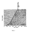
- FIGURE 1 An example of seismic data which shows 1500 milliseconds (msec) of a 500 millisecond normalizing window beginning at zero time is illustrated in FIGURE 1.
- data begins to be received by the various geophones (each wiggle trace is supplied from a different geophone set) at different times.
- the first normalizing window is begun at a fixed time, such as zero time, then it can be seen that no valid information would be present (dominantly zeros) on the upper wiggle traces. This has an adverse affect on the normalizing procedure which will be described hereinafter and thus, the first window is given a length of zero to the first break time interval.
- the start for the first normalizing window is preferably set as illustrated in FIGURE 1. It should be remembered that the 500 ms window should be measured in reference now to the window start time and not the wiggle trace zero time.
- First break time is defined as that time data is first received at the geophone.
- Seismic wiggle traces such as those illustrated in FIGURE 1, are conventionally in digital format. In this step, the average amplitude of each digital format window is determined.
- a normalizing value is selected by the interpreter (this value is referred to hereinafter as the "normalizing constant"). Any desired normalizing constant can be used based on the size of the resultant normalized data number desired.
- a typical normalizing constant is 10.
- the average determined in Step 2 is then divided into the normalizing constant determined by the interpreter in this Step 3 to determine a multiplier. All of the amplitudes for the seismic wiggle traces in the window are then multiplied by such multiplier to normalize each amplitude. These are the data values used in the crossplot.
- the derivative of the seismic wiggle trace for each data point is determined.
- An average derivative for the window is then determined. Typically, for a 4 millisecond sample rate, this average will be about one-half of the average determined in Step 2 above and, even at different sample rates, will always be less than the average determined in Step 2 above.
- any desired method may be utilized to determine the derivative. Methods such as backward difference, forward difference, central difference or the Hilbert transform are suitable. A 2 point forward difference or backward difference calculation is preferred because it has the advantage of allowing a noise spike to affect the slope (derivative) calculation at the spike value and at only one adjacent sample. Further, such calculation is relatively simple and is more rapidly computed than a central difference or other derivative methods. The resultant slope is the slope of a point between the two data points and not the data point.
- the backward difference refers to the slope between the previous data point and the data point being analyzed.
- the forward difference refers to the slope between the data point being analyzed and the next data point in time.
- a central difference refers to the average of the backward difference and forward difference and is the slope of the data point itself.
- Step 4 The average determined in Step 4 above is divided into the normalizing constant selected in Step 3 to determine a second multiplier. All derivative values in the window are then multiplied by this second multiplier to normalize the derivative to the same reference values as the amplitude. These are the data used in the crossplot.
- the normalized amplitude (ordinate) and normalized derivative (abscissa) are crossplotted. As has been previously stated, and as will be more fully illustrated in the examples, actual seismic data will tend to cluster at the center of the crossplot. If the absolute values of the normalized data are used all the plots will fall in the first quadrant of the crossplot. Under this condition actual seismic data will tend to cluster around the origin as illustrated in FIGURE 11.
- rejection radius any desired radius of the circle (referred to "rejection radius") can be utilized.
- the rejection radius will typically be in the range of about 3 times the normalizing constant to about 6 times the normalizing constant.
- a rejection radius in the range of about 4 times the normalizing constant to about 4.5 times the normalizing constant is generally an effective choice.
- a 2 + D 2 is greater than R 2 , then it is necessary to assign a new amplitude to the data point since the old amplitude is a result of noise. Any desired method may be utilized to assign such a new value. Generally, such data points are either zeroed or reinterpolated. A preferred method of reassigning values to data points which are rejected under equation 1 is as follows:
- Steps 1-8 or a desired portion of Steps 1-8 may be repeated several times for the same data if desired. Such multiple passes results in an improved removal of noise.
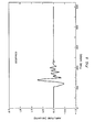
- FIGURE 2 illustrates a computer generated sinusoidial data trace.
- random noise spikes have been added to the trace illustrated in FIGURE 2.
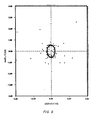
- FIGURE 4 illustrates a normalized derivative versus normalized amplitude crossplot of the trace illustrated in FIGURE 3. The sample rate was 4 msec.
- FIGURE 5 Data points outside the rejection circle 1 illustrated in FIGURE 4 represent noise. These data points were treated according to the procedure described in Step 8. After such treatment, the trace was regenerated and is illustrated in FIGURE 5. It can be seen that the reconstructed data of FIGURE 5 compares very favorably with the original data of FIGURE 2.
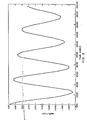
- FIGURE 6 shows a linearly damp 20 Hertz cosine wave.
- FIGURE 7 four anomalous, subtle spikes have been added at points A, B, C and D.
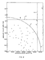
- a crossplot of the absolute value of derivative versus amplitude for the waveform illustrated in FIGURE 7 is illustrated in FIGURE 8. All data is in the first quadrant.
- the maximum amplitude of the trace will be 1 and, allowing for some variation, the acceptable maximum amplitude has been assumed to be 1.05.
- the maximum derivative of the trace will be .5 and, allowing for some variation, the acceptable maximum derivative has been assumed to be .55.
- These acceptable values are indicated by values below and/or to the left of the lines 3 and 5, respectively.
- Point A is rejected by either amplitude or derivative as it lies above the 1.05 horizontal line 3 and to the right of the .55 vertical line 5.
- Point B is rejected by amplitude criteria but not by derivative criteria.
- Point C is rejected by derivative criteria only.
- Point D is marginal and is not rejected by either amplitude or slope criteria alone or in combination.
- the rejection radius 7 in FIGURE 8 allows larger variation allowances for the acceptable values (1.1 for the amplitude and .6 for the derivative).
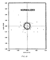
- FIGURES 9 and 10 illustrate the effect of normalization.
- the crossplotted data was not normalized.
- FIGURE 10 the same data plotted in FIGURE 9 was normalized and then crossplotted.
- the ellipse formed by the data of FIGURE 9 has become nearly circular in FIGURE 10.
- the ellipse and circle in the figures are not actual rejection radii but only data point clusters.
- FIGURES 9 and 10 the data is shown as clustered along an ellipse or a circle. In real seismic data this would generally not be the case.
- the wide variation of amplitudes and frequencies cause the crossplotted points to cluster within a central area rather than plot along an ellipse or a circle.
- noise values still migrate outside the central area.
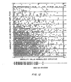
- FIGURES 11 and 12 are actual printouts, representative of the absolute values of normalized amplitude and absolute values of normalized derivative of a trace, produced by the computer programs described hereinafter. These figures illustrate the effect of the normalizing window length.
- the data crossplotted in each case is identical with the numbers representing the number of data points at that matrix location. For example, 0 means 10 or more data points plot at that location. It can be seen that, at the greater window length, the percentage of the data rejected for any given rejection radius is greater.
- M on each axis refers to the normalizing constant value described in Step 3 above.
- 3 X refers to 3 times M (the normalizing constant value selected in Step 3 above). The rejection radius then is selected between 3 to 6 times M.
- the derivative and amplitude are preferably normalized to the same normalizing constant such that the normalized average derivative to normalized average amplitude ratio is equal to 1.0.
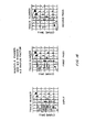
- FIGURES 13, 14 and 15 which are similar to FIGURES 11 and 12. It can be seen that doubling the ratio, which is illustrated in FIGURE 14, results in a higher rejection of data. The data clusters move along the derivative axis thus causing more rejection due to the derivative criteria.
- halving of the ratio also results in a higher higher rejection of data due to the clustering of the data along the amplitude axis (amplitude criteria).
- the use of non-unity ratios will cause the rejection criteria to be more amplitude dependent for ratios less than 1.0 or more derivative dependent for ratios greater than 1.0.
- FIGURE 16 An example of a multiple pass is illustrated in FIGURE 16. The effect of the multiple pass is particularly pronounced for the seismic wiggle trace at the left.
- the preferred computer program for accomplishing Steps 1-8 which crossplots the seismic data and then removes noise from the seismic data is set forth in Appendix 1.
- the computer program is written for an IBM 4341 computer manufactured by IBM and is self explanatory to one skilled in the use of the IBM 4341 computer.
- the input required into the computer program is the seismic data, in digital form, the window length, the window start time, the sample rate and the derivative/amplitude ratio.
Landscapes
- Physics & Mathematics (AREA)
- Engineering & Computer Science (AREA)
- Life Sciences & Earth Sciences (AREA)
- Environmental & Geological Engineering (AREA)
- Remote Sensing (AREA)
- General Physics & Mathematics (AREA)
- Emergency Management (AREA)
- Business, Economics & Management (AREA)
- Acoustics & Sound (AREA)
- Geology (AREA)
- General Life Sciences & Earth Sciences (AREA)
- Geophysics (AREA)
- Geophysics And Detection Of Objects (AREA)
- Apparatus For Radiation Diagnosis (AREA)
Applications Claiming Priority (2)
| Application Number | Priority Date | Filing Date | Title |
|---|---|---|---|
| US58944684A | 1984-03-14 | 1984-03-14 | |
| US589446 | 1984-03-14 |
Publications (3)
| Publication Number | Publication Date |
|---|---|
| EP0182956A2 true EP0182956A2 (fr) | 1986-06-04 |
| EP0182956A3 EP0182956A3 (en) | 1988-01-13 |
| EP0182956B1 EP0182956B1 (fr) | 1990-12-12 |
Family
ID=24358060
Family Applications (1)
| Application Number | Title | Priority Date | Filing Date |
|---|---|---|---|
| EP19850102621 Expired EP0182956B1 (fr) | 1984-03-14 | 1985-03-07 | Traitement de données |
Country Status (6)
| Country | Link |
|---|---|
| EP (1) | EP0182956B1 (fr) |
| AU (1) | AU560198B2 (fr) |
| CA (1) | CA1227576A (fr) |
| DE (1) | DE3580902D1 (fr) |
| NO (1) | NO851020L (fr) |
| PH (1) | PH23998A (fr) |
Cited By (1)
| Publication number | Priority date | Publication date | Assignee | Title |
|---|---|---|---|---|
| EP0354813A3 (fr) * | 1988-08-11 | 1991-05-29 | Western Atlas International, Inc. | Procédé de traitement de données sismiques |
Family Cites Families (1)
| Publication number | Priority date | Publication date | Assignee | Title |
|---|---|---|---|---|
| US4218765A (en) * | 1974-10-03 | 1980-08-19 | Standard Oil Company (Indiana) | Two-dimensional frequency domain filtering |
-
1985
- 1985-01-21 CA CA000472514A patent/CA1227576A/fr not_active Expired
- 1985-03-07 EP EP19850102621 patent/EP0182956B1/fr not_active Expired
- 1985-03-07 DE DE8585102621T patent/DE3580902D1/de not_active Expired - Fee Related
- 1985-03-12 PH PH31977A patent/PH23998A/en unknown
- 1985-03-14 AU AU39868/85A patent/AU560198B2/en not_active Ceased
- 1985-03-14 NO NO851020A patent/NO851020L/no unknown
Cited By (1)
| Publication number | Priority date | Publication date | Assignee | Title |
|---|---|---|---|---|
| EP0354813A3 (fr) * | 1988-08-11 | 1991-05-29 | Western Atlas International, Inc. | Procédé de traitement de données sismiques |
Also Published As
| Publication number | Publication date |
|---|---|
| PH23998A (en) | 1990-02-09 |
| EP0182956A3 (en) | 1988-01-13 |
| AU560198B2 (en) | 1987-04-02 |
| AU3986885A (en) | 1985-09-19 |
| EP0182956B1 (fr) | 1990-12-12 |
| DE3580902D1 (de) | 1991-01-24 |
| CA1227576A (fr) | 1987-09-29 |
| NO851020L (no) | 1985-09-16 |
Similar Documents
| Publication | Publication Date | Title |
|---|---|---|
| Stainsby et al. | Q estimation from vertical seismic profile data and anomalous variations in the central North Sea | |
| US7616524B1 (en) | Wavelet based intercept attribute for seismic exploration | |
| US5193077A (en) | Method and apparatus for improved seismic prospecting | |
| US20090285052A1 (en) | Methods of enhancing separation of primary reflection signals and noise in seismic data using radon transformations | |
| US4757480A (en) | Method and apparatus for filtering seismic data | |
| Blandford | Seismic event discrimination | |
| EP0782011A2 (fr) | Corriger les effets de différences de couplage dans les mesures seismiques | |
| US5287328A (en) | Method for removing random source and receiver noise from seismic traces | |
| Kennett et al. | Vertical seismic profiles: Their applications in exploration geophysics | |
| EP1532472B1 (fr) | Elimination de bruit de donnees sismiques au moyen de transformations de radon ameliorees | |
| US4688198A (en) | Entropy guided deconvolution of seismic signals | |
| US4885711A (en) | Data processing | |
| Wassermann | Locating the sources of volcanic explosions and volcanic tremor at Stromboli volcano (Italy) using beam-forming on diffraction hyperboloids | |
| Klemperer | Seismic noise-reduction techniques for use with vertical stacking; an empirical comparison | |
| US4532618A (en) | System for and method of processing a seismic signal | |
| US5442591A (en) | Method for adaptively suppressing noise transients in summed co-sensor seismic recordings | |
| EP0182956B1 (fr) | Traitement de données | |
| US4755972A (en) | Method of seismic exploration including processing and displaying shear wave seismic data | |
| US4476551A (en) | Selecting offset as a function of time and velocity to stack seismograms with high signal to noise ratio | |
| Paulson et al. | Automatic seismic reflection picking | |
| EP0169321A2 (fr) | Détermination de déphasage par traitement numérique | |
| Filson | Array seismology | |
| Bullitt et al. | The relative performance of mb and alternative measures of elastic energy in estimating source size and explosion yield | |
| Behura | Virtual real source | |
| Graebner | Seismic data enhancement—A case history |
Legal Events
| Date | Code | Title | Description |
|---|---|---|---|
| PUAI | Public reference made under article 153(3) epc to a published international application that has entered the european phase |
Free format text: ORIGINAL CODE: 0009012 |
|
| AK | Designated contracting states |
Kind code of ref document: A2 Designated state(s): BE DE FR GB IT NL |
|
| PUAL | Search report despatched |
Free format text: ORIGINAL CODE: 0009013 |
|
| RHK1 | Main classification (correction) |
Ipc: G01V 1/36 |
|
| AK | Designated contracting states |
Kind code of ref document: A3 Designated state(s): BE DE FR GB IT NL |
|
| 17P | Request for examination filed |
Effective date: 19880613 |
|
| 17Q | First examination report despatched |
Effective date: 19890825 |
|
| GRAA | (expected) grant |
Free format text: ORIGINAL CODE: 0009210 |
|
| AK | Designated contracting states |
Kind code of ref document: B1 Designated state(s): BE DE FR GB IT NL |
|
| ITF | It: translation for a ep patent filed | ||
| ET | Fr: translation filed | ||
| REF | Corresponds to: |
Ref document number: 3580902 Country of ref document: DE Date of ref document: 19910124 |
|
| PGFP | Annual fee paid to national office [announced via postgrant information from national office to epo] |
Ref country code: GB Payment date: 19910221 Year of fee payment: 7 |
|
| PGFP | Annual fee paid to national office [announced via postgrant information from national office to epo] |
Ref country code: FR Payment date: 19910224 Year of fee payment: 7 |
|
| PGFP | Annual fee paid to national office [announced via postgrant information from national office to epo] |
Ref country code: DE Payment date: 19910227 Year of fee payment: 7 |
|
| ITTA | It: last paid annual fee | ||
| PGFP | Annual fee paid to national office [announced via postgrant information from national office to epo] |
Ref country code: NL Payment date: 19910331 Year of fee payment: 7 |
|
| PGFP | Annual fee paid to national office [announced via postgrant information from national office to epo] |
Ref country code: BE Payment date: 19910415 Year of fee payment: 7 |
|
| PLBE | No opposition filed within time limit |
Free format text: ORIGINAL CODE: 0009261 |
|
| STAA | Information on the status of an ep patent application or granted ep patent |
Free format text: STATUS: NO OPPOSITION FILED WITHIN TIME LIMIT |
|
| 26N | No opposition filed | ||
| PG25 | Lapsed in a contracting state [announced via postgrant information from national office to epo] |
Ref country code: GB Effective date: 19920307 |
|
| PG25 | Lapsed in a contracting state [announced via postgrant information from national office to epo] |
Ref country code: BE Effective date: 19920331 |
|
| BERE | Be: lapsed |
Owner name: PHILLIPS PETROLEUM CY Effective date: 19920331 |
|
| PG25 | Lapsed in a contracting state [announced via postgrant information from national office to epo] |
Ref country code: NL Effective date: 19921001 |
|
| GBPC | Gb: european patent ceased through non-payment of renewal fee | ||
| NLV4 | Nl: lapsed or anulled due to non-payment of the annual fee | ||
| PG25 | Lapsed in a contracting state [announced via postgrant information from national office to epo] |
Ref country code: FR Effective date: 19921130 |
|
| PG25 | Lapsed in a contracting state [announced via postgrant information from national office to epo] |
Ref country code: DE Effective date: 19921201 |
|
| REG | Reference to a national code |
Ref country code: FR Ref legal event code: ST |