EP0439935A2 - Optimale Steuerung für stochastische LP-Systeme - Google Patents
Optimale Steuerung für stochastische LP-Systeme Download PDFInfo
- Publication number
- EP0439935A2 EP0439935A2 EP90313600A EP90313600A EP0439935A2 EP 0439935 A2 EP0439935 A2 EP 0439935A2 EP 90313600 A EP90313600 A EP 90313600A EP 90313600 A EP90313600 A EP 90313600A EP 0439935 A2 EP0439935 A2 EP 0439935A2
- Authority
- EP
- European Patent Office
- Prior art keywords
- matrix
- signal
- output
- vector
- input port
- Prior art date
- Legal status (The legal status is an assumption and is not a legal conclusion. Google has not performed a legal analysis and makes no representation as to the accuracy of the status listed.)
- Withdrawn
Links
Images




Classifications
-
- G—PHYSICS
- G05—CONTROLLING; REGULATING
- G05B—CONTROL OR REGULATING SYSTEMS IN GENERAL; FUNCTIONAL ELEMENTS OF SUCH SYSTEMS; MONITORING OR TESTING ARRANGEMENTS FOR SUCH SYSTEMS OR ELEMENTS
- G05B13/00—Adaptive control systems, i.e. systems automatically adjusting themselves to have a performance which is optimum according to some preassigned criterion
- G05B13/02—Adaptive control systems, i.e. systems automatically adjusting themselves to have a performance which is optimum according to some preassigned criterion electric
Definitions
- This invention relates to the control of stochastic processes or systems in order to meet, maximize, or minimize specified performance criteria. More particularly, this invention relates to method and apparatus for optimizing a selected performance criterion of the process or system under control, such as the criterion of optimizing resource allocation costs.
- the dynamics of a given system or process can be completely described in terms of the "states" of the system or process.
- the dynamics of an electric motor can be described in sufficient detail by the angular displacement, the angular velocity, and the angular acceleration of its rotating shaft.
- the various sets of values of these three parameters can be thought of as the states of the system.
- These parameters may be directly measurable (such as the speed measured with a tachometer) or may be indirectly measurable, and control of systems can be based on those measurements.
- the observed measurements may be corrupted by operational and measurement noise. Systems that include such noise components are typically referred to as stochastic systems.
- Stochastic systems can be controlled with an approach that comprises an observer system and a separate observer-responsive controller system.
- the concept is to deduce the states of the system under consideration by using an observer system and then to synthesize a control signal strategy that would control and consequently change the output of the system based on the observed states.
- the observer system estimates the various states of the system from transducer-provided samples of inputs and outputs of the system. For example, in observing the states of a chemical process, thermocouples can measure the temperatures in different parts of a chemical plant to give an indication of the states of the chemical plant.
- Kalman filter In handling the observations of stochastic systems artisans have typically employed the Kalman filter as a stochastic observer (Kalman, R.E., "A New Approach to Linear Filtering and Prediction Problems", Transactions of the A.S.M.E., Journal of Basic Engineering, Vol.82, pp. 35-45,1960).
- the Kalman filter filters out the stochastic component of the observed parameters and outputs the expected value of those parameters.
- DP dynamic programming
- the observer-responsive controller system can use the same hardware or software when handling problems that can he solved by DP; that is, problems where the cost function is quadratic. This substantially reduces the cost of developing the overall controller system, whether it is implemented in hardware or in software (i.e., in a stored program controlled processor).
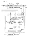
- FIG. 1 presents the prior art control arrangement of a stochastic system. It includes a representation of the system under control and the control apparatus.
- the symbolic representation of the "system under control” encompasses noise-free system 10, process noise 11 and observation noise 12.
- Process noise 11 is applied to system 10, the observation noise is added to the output of system 10 via adder 14, and the result forms the observable output 13 of the system.
- Observer system 20 is responsive to output 13. It develops an estimate of the state of system 10. That is the Kalman filter. The estimate developed by the Kalman filter is applied to observer-responsive controller system 30 which develops the control signals for improving the a prior selected performance criteria of system 10. Lastly, the control signals are applied to system 10 to force it in the direction that improves the aforementioned performance criteria.
- System 10 can be a simple servo motor system but it certainly can be more complicated as well. It can be a chemical plant whose energy use one wishes to optimize, an airline enterprise whose fuel consumption one wishes to optimize, a communications enterprise whose transmission capacity one wishes to utilize efficiently, etc.
- z (t) is an n dimension state vector
- F is an n ⁇ n state transition matrix
- G is an n ⁇ m input matrix
- H is a k ⁇ n output matrix
- u (t) is an m dimensional control input vector
- v (t) is an n dimensional system noise
- y (t) is a k dimensional measured output
- e (t) is a k dimensional measurement noise.
- the vector z (t+1) has n components and each component represents one of the observable attributes of system 10. This can be temperature, pressure, weight, acceleration, etc. Taking the components as a group, the vector z (t+1) represents the state of system 10 at time t+1.
- the vectors u (t) and y (t) are the system inputs and outputs respectively. That is, u (t) is the set of input signals at time t that are applied to system 10, and y (t) is the set of output signals at time t that appear on line 13.
- the matrix F describes the input/output relationships of the system.
- the matrix F describes the movement of the system from the a state at time t, i.e., z (t), to a state at time t+1, i.e., z (t+1).
- the matrix G describes the effect of an input signal on the various components of z (t)
- the matrix H describes the relationship between the observable parameters and the actual output of the system, y (t).
- the states of system 10 in the presence of noise components 11 and 12 can be estimated by using a Kalman filter 20. It can be shown that the filter provides minimum variance estimates of the state z (t) of system 10 (i.e., minimizes the norm
- the Kalman filtering proceeds as follows:
- the above-described Kalman filtering procedure may be carried out in the system of FIG. 1 with the circuitry depicted within block 20.
- the observable output, y (t) is stored in memory 21 and the input, u (t), is stored in memory 22.
- Memories 21 and 22 store a select number of the latest samples of y (t) and u (t). The number of stored samples affects the Kalman filter by fixing the "history" span on which the estimates developed by the filter are based. This span is also called “the control horizon.” These samples are accessed under control of the test & control block 23 (the control path is not shown in FIG. 1 to reduce complexity) and applied to processors 24 and 25.
- Kalman filter 20 receives characterizing information about system 10 "off line", and that information is stored in the memory blocks marked F, H, G, Q, and R (corresponding to the information stored therein).
- Processor 24 develops a signal representative of equation (2a)
- processor 26 develops a signal representative of equation (2b)
- processor 27 develops a signal representative of equation (2c)
- processor 25 develops a signal representative of equation (2d)
- processor 28 develops a signal representative of equation (2e).
- Registers 31 and 32 provide a one sample delay to yield signals P (t-1/t-1) and and deliver their output to processors 24 and 26, respectively.
- control block 23 Under control of block 23, the signals of registers 31 and 32 combine with the signals of memories 21 and 22 (and all the processing in between) to form an estimate of the state of system 10.
- gate 33 permits the estimated output of system 10 to exit Kalman filter 20.
- the estimated system state of filter 20 is then applied to controller 30 to develop control signals for affecting the operation of system 10.
- the Kalman filter of FIG. 1 can be implemented in a number of ways.
- the two primary techniques are special purpose hardware and program controlled general purpose processor hardware.
- the latter approach has become more economical in recent years because of the lower cost and higher speeds of general purpose processors.
- processor 27 that creates the signal that corresponds to equation (2c). It needs routines for the matrix inversion; but such routines are readily available in the art.
- observer-responsive controller 30 is often implemented through dynamic programming. Its operation is outlined below for sake of completeness, though more complete descriptions are available in the art, as indicated above.
- Obtaining the signals for controlling system 10 in accordance with dynamic programming techniques proceeds along the following lines. Since it is known that the system under control moves from one state to another state in response to a driving signal, it follows that each state leads to a number of other states, depending on the value of the driving signal. The objective, then, is to move the system from its given initial state, through intermediate starts, to a goal state, at the least cost.
- x (k) is an interior point within the polytope (i.e. a feasible solution of the LP problem) at iteration k of the affine scaling algorithm
- D x (k) is the diagonal matrix containing the components of x (k)
- the translation vector c p (k) that directs the movement of the system from x (k) to a new feasible point x (k+1) is given by and the new feasible point is given by
- the vector e i is i-th unit vector, which is a vector of all 0s except for a 1 in the i th component thereof.
- Equations (3e) and (3b) can also be written as With each iteration of the affine scaling algorithm where a new feasible point is evaluated, a test is performed to determine whether an additional iteration is necessary. If it is, the newly developed x (k+1) becomes the new x (k) and the process repeats. When it is determined that additional iterations are no longer necessary, the value of x (k) is transmitted to the system that is being controlled.
- the above-described affine scaling algorithm is implementable with modules that iteratively perform processing to develop signals corresponding to equations 3 and 4. More specifically, the affine scaling processor is sometimes implemented with modules that store the A, c and b information (somewhat akin to the memory modules that receive the F information in FIG. 1), and processing modules that operate on the given information.
- the collection of processing modules includes a module for evaluating the value of w (k) (equation 3d), a module responsive to the developed w (k) for evaluating ⁇ (equation 4a), a module responsive to the developed w (k) for developing the value of x (k+1), a test module a-1a circuit 23 in FIG.
- Another difficulty is that the parallelism between the conventional Kalman filter observer and the controller is lost when one chooses a performance criterion other than the quadratic one. That is a substantial difficulty because in industry there are many control problems that neither lend themselves to, nor advantageously should, be modeled with a quadratic cost function.
- "Minimum time” problems form one class of such control problems. Unlike “minimum energy” problems where the objective is to conserve fuel, or energy, the objective in "minimum time” problems is to reach the desired terminal state of the system under control in the least possible time.
- a specific example of a "minimum time” problem is the flight control of a military missile. Typically, it is more important for the missile to reach its target in the minimum possible time than to conserve fuel.
- Our invention makes use of the conceptual and computational similarities between the Karmarkar method as described in US patent 4,744,028, issued May 10,1989 and the Kalman filter by developing a controller system that is capable of handling the observer function and the minimum time controller function for stochastic systems.
- the system includes an element that has the computational structure of a Kalman filter but the inputs of this element are qualitatively controlled to deliver the desired results to the remaining computation elements.
- our system performs iterative computations in accordance with the interior point affine scaling algorithm.
- the "dual vector" of the affine scaling algorithm is computed in the Kalman filter structure element by applying information to it as if its task were to estimate the states of a hypothetical system whose observable output is D x(k) c, the input is O, the system noise covariance matrix of the hypothetical system corresponds to the system noise of the stochastic LP system under control, the measurement noise covariance matrix of the hypothetical system corresponds to the measurement noise of the stochastic system under control, the transition matrix of the hypothetical system is I and the matrix that describes the relationship between the measurable parameters and the observable output of the hypothetical system is A T D x(k) .
- the value of w (k) in equation 3(d) is a least squares solution.
- the developed value of the dual vector w (k) is one that minimizes
- the state vector estimate in a Kalman filter arrangement is a least square estimate of the state vector z (t), where z (t) is the true state vector and is the filtered state vector. That is, the developed value of is one that minimizes
- equation (5a) We also discovered that equation (4) can be rewritten as and in this form, equation (5b) corresponds to equation (1b) when the following variable substitutions are made: y (t) ⁇ D x (k) c (6a) H ⁇ D x (k) A T (6b) z (t) ⁇ w (k) (6c) and With these substitutions in place, various conceptual and computational parallelisms between the two techniques can be brought to light.
- the filtered state vector developed by a Kalman filter is equal to the dual vector of the affine scaling algorithm.
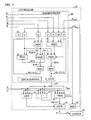
- FIG. 3 presents an illustrative block diagram of this implementation.
- system 40 may be any commercial or industrial system that utilizes resources in the course of its operation and that is characterized by an expense that is involved with such utilizing of resources.
- the objective is to reduce the expenses in accordance with a cost function that is characteristic of system 40.
- the controller that sends commands to system 40 is a feed-forward controller. It does not have a feedback path to allow controlling of system 40 based on its present state.
- the interior point method invented by Karmarkar requires an initial, feasible, starting point
- the present operating point of system can be fed to the controller to serve as that initial, feasible, starting point. This may speed the computations for developing the optimizing control signals.
- the FIG. 3 embodiment is simply a realization of the affine scaling optimization algorithm for an LP problem associated with a non-stochastic system that is controlled in a feed-forward manner.
- the LP affine scaling algorithm controller of system 40 comprises blocks 60 and 51-56. More specifically, block 60 in FIG. 3 develops the dual vector w (k) that corresponds to equation (3d). Block 51 computes the value of ⁇ based on the value of w (k), A, D x (k) and c in accordance with equation (4a). Processor 52, responsive to w (k), ⁇ , c, A, and D x (k) develops the next value, x (k+1), in accordance with equation (4b). It also develops the diagonal matrix for this new value of x (k+1), multiplied by the cost vector c, and stores that value in register 56 for the next iteration as an input to block 60.
- Block 53 performs the test of equation (4c) based on the value of w (k), A, c and D x (k) , and it determines whether the iterations that encompass blocks 60, 51, 52, and 56 should continue.
- gate 54 is enabled to allow the value of the vector x to be applied to system 40.
- block 60 develops the dual vector of w (k) with a Kalman filter that is identical in structure to the filter described in FIG. 1.
- the difference lies in the fact that the Kalman filter is made to estimate the state of a hypothetical system or, more particularly, the difference lies in the signals that are applied to the Kalman filter of FIG. 3.
- the input to the blocks that maintain the R matrix is ⁇ I , where ⁇ is a selected constant close to 0 (to insure computational stability).
- the input to the block that maintains the Q matrix is 0 .
- the input to the block that maintains the H matrix is the matrix that corresponds to A T D x (k)
- the input to the block that maintains the F matrix is I .
- either the input to the block that maintains the G matrix is 0, or the input to the memory that receives the input signal u (t) in FIG. 1 is 0 (or both), and the input to the memory that received the observed output signal y (t) in FIG. 1 is D x (k) c .
- the QP algorithm proceeds as follows.
- the controller depicted in Fig. 3 is applicable to optimization of a system 40 where the cost function is linear; and the controller depicted in FIG. 4, which is essentially identical to that of FIG. 3 but with different inputs, is applicable to optimization of a system 40 where the cost function is quadratic.
- FIG. 3 and FIG. 4 embodiments implement the affine scaling algorithm (for LP and QP, respectively) with the aid of a Kalman filter in the context of a feed-forward control arrangement.
- some systems are best controlled with a feedback loop because the system is not static.
- the concept of a system being "static” or “changing” is a relative concept.
- Some systems are static enough so that LP problem can be formulated and solved and that solution in essence remains valid throughout some sufficiently long period of time.
- the system under control changes too often in relation to the time it takes to develop control signals, or changes in a way we don't understand. Those systems we call varying or stochastic.
- Variations in a system are, in effect, changes in the basic constraint relationships in the system under control and/or on the limits on the constraints.
- the parameters representing A, c and b change in that system; and with each change a new solution for the optimal state must be found.
- the elements of A and b are observable in that the user can set up a communications path for supplying the observer/controller with the information about the needs and constraints of the system. In a chain of stored, for example, this may comprise an automated inventory control system.
- This observable information can be stochastic. Some of the observable elements may be observed without noise but others may be "noisy". An observation may be considered "noisy" when it is known that the observation, though accurately recorded, tends to change from time to time, and that a better result would be attained if it were assumed that the observation has a stochastic component. Other observable elements may have a stochastic component in that the user informs the observer/controller that the system's requirements are flexible.
- the cost information which is supplied to the controller may also be changing from time to time and, in fact, it may be known that the cost information may have a stochastic component.
- the cost of oil from a particular source may change slowly with demand and geo-political conditions, but may also have a stochastic component that is a function of the weather through which the oil tankers must traverse.
- stochastic components that is a function of the weather through which the oil tankers must traverse.
- the situation resembles the one described in connection with FIG. 1.
- the observed states are estimated with an observer system to provide an estimate of A, b, and c .
- the observer function is performed, then the two situations become identical; to wit, values for A, b, and c are known and it is also known that A, b, and c are noisy with covariance matrices Q and R .
- the covariance matrix information is advantageously utilized in the controller by supplying the stochastic information to the Kalman filter of the FIG. 3 embodiment.
- FIG. 5 shows these modified inputs to the controller of FIG. 3.
- FIG. 6 depicts the complete feedback arrangement where the system under control provides the information about the parameters of the system.
- FIG. 6 includes a modeling module 25 which is responsive to the system under control.
- module 25 is an observer system that observes the outputs of the system under control and conditions the derived information to the desried form.
- the output of modeling module 25 is the A, b, and c information as well as the stochastics information that describes the measurement noise and the system noise; i.e. the covariance matrices R and Q .
- Controller 30 receives the A, b, and c information and, in accordance with the principles of our invention, also receives the Q and R information.
- the control signals developed by controller system 30 are affected by those Q and R signals as described above.
- modeling block 25 is to develop an appropriate model of the system under control in terms of an LP system ( A, b, and c ).
- the means for accomplishing this are widely known.
- a good reference in this area is the book by Sinha and Kuszta, "Modeling and Identification of Dynamic Systems", published by Van Nostrand and Reinhold company in 1983.
- the controller of FIG. 3 is shown to include a Kalman filter and a number of additional components. Although it is presumed that in realizing the controller artisans would simply purchase a Kalman filter, FIGS. 1-5 present sufficient information to allow a skilled artisan to create the filter "from scratch". That is, as suggested earlier, each of the processors in the Kalman filter can be created for the specific computational function that it needs to perform or, alternatively, each of the processors can be realized with a general purpose processing element, such as a microprocessor, with attendant memory and stored program control. The same applies to the processors outside the Kalman filter that are included in the controller of FIG. 3.
- FIG. 3 controller can be implemented in a single general purpose computer, under program control, and the program control can even include a switch function to allow the processor to A. execute a normal Kalman filter that carries out the observer function, as needed for the arrangement of FIGS. 1, B. execute the Kalman filter function per equation (6), together with the remainder of the affine scaling algorithm -- to solve an LP problem, or C. execute the Kalman filter function per equation (14), together with the remainder of the affine scaling algorithm -- to solve a QP problem.
- the process of controlling such a general purpose processor is shown in the form of a flow chart in FIG. 7.
- the first step (301) is to model the system or process to be controlled as a linear discrete-time state space representation as depicted by equations (1a) and (1b). This could be done from the dynamics of the system or by empirical methods. As indicated above, the methods for such modeling are widely known. This modeling process is, of course, not part of the direct process of control. It is an "off line" step that is the predicate to the control process. Once the modeling part is done, the information describing the model is installed in the Kalman filter, in accordance with equations (equations 2a through 2e).
- the filter then responds to the output signals of the system under control (signals 303) and develops estimates of the system state in step 302.
- the system state estimate is converted to the LP model representation in process 312.
- decision process 305 determines whether a minimum time (306) or a minimum energy (307) control strategy is employed, and applied the developed states to process 308 or to process 309.
- the LP based controller of equation (6) is implemented, and in process 309 the QP based controller of equation (14) is implemented.
- FIG. 8 illustrates the stochastic LP solver set up based on the unified three-in-one observer/controller system, in accordance with the principles of our invention.
- Block 401 is the system or process to be controlled.
- Blocks 402 and 412 include appropriate transducers which generate electrical signals corresponding to the input and output of the system, respectively. These electrical signals are often analog in nature and, hence, blocks 403 are provided, which are analog-to-digital converts that make these signals ready for use by a digital computer.
- Signal lines 404 carry this digital data to element 405, which is a digital computer.
- computer 405 Upon the arrival of the data, computer 405 invokes the Kalman filter by setting appropriate parameters in the common software 406 residing in the memory of the computer, and estimates the states of the system. Setting of the parameters in software 406 is tantamount to applying the appropriate inputs to the Kalman filter, as depicted in FIGS. 3 and 4.
- the information on the states estimated by computer 405 is displayed on the console 408 of the computer for human monitoring.
- the console is also used to provide input to computer 405 on the type of control action to be taken (minimum time or minimum energy) and the corresponding parameters (desired output, control horizon, penalty for deviating from desired output goal, limits on control input, etc.) to be used in deploying the selected control strategy.
Landscapes
- Engineering & Computer Science (AREA)
- Health & Medical Sciences (AREA)
- Artificial Intelligence (AREA)
- Computer Vision & Pattern Recognition (AREA)
- Evolutionary Computation (AREA)
- Medical Informatics (AREA)
- Software Systems (AREA)
- Physics & Mathematics (AREA)
- General Physics & Mathematics (AREA)
- Automation & Control Theory (AREA)
- Feedback Control In General (AREA)
- Management, Administration, Business Operations System, And Electronic Commerce (AREA)
Applications Claiming Priority (2)
| Application Number | Priority Date | Filing Date | Title |
|---|---|---|---|
| US47125390A | 1990-01-26 | 1990-01-26 | |
| US471253 | 1990-01-26 |
Publications (2)
| Publication Number | Publication Date |
|---|---|
| EP0439935A2 true EP0439935A2 (de) | 1991-08-07 |
| EP0439935A3 EP0439935A3 (en) | 1992-04-15 |
Family
ID=23870879
Family Applications (1)
| Application Number | Title | Priority Date | Filing Date |
|---|---|---|---|
| EP19900313600 Withdrawn EP0439935A3 (en) | 1990-01-26 | 1990-12-13 | Optical control for stochastic lp systems |
Country Status (2)
| Country | Link |
|---|---|
| EP (1) | EP0439935A3 (de) |
| JP (1) | JPH052403A (de) |
Cited By (4)
| Publication number | Priority date | Publication date | Assignee | Title |
|---|---|---|---|---|
| WO1995034850A3 (en) * | 1994-06-16 | 1996-02-01 | Litton Systems Inc | Assured-integrity monitored-extrapolation navigation apparatus |
| NL1001100C2 (nl) * | 1994-08-31 | 1999-01-05 | Exxon Production Research Co | Inrichting en werkwijze voor het lokaliseren van een bron van akoestische golven. |
| EP1426840A1 (de) * | 2002-12-02 | 2004-06-09 | United Technologies Corporation | Quadratische Echtzeitprogrammierung zur Steuerung von dynamischen Systemen |
| WO2004049080A1 (en) * | 2002-11-21 | 2004-06-10 | Honeywell International Inc. | Energy forecasting using model parameter estimation |
Families Citing this family (2)
| Publication number | Priority date | Publication date | Assignee | Title |
|---|---|---|---|---|
| KR101234797B1 (ko) | 2006-04-04 | 2013-02-20 | 삼성전자주식회사 | 로봇 및 산출된 공분산을 이용한 로봇의 위치 추정 방법 |
| JP5740433B2 (ja) * | 2013-05-24 | 2015-06-24 | 日本電信電話株式会社 | 遅延補償装置、方法、プログラム及び記録媒体 |
Family Cites Families (2)
| Publication number | Priority date | Publication date | Assignee | Title |
|---|---|---|---|---|
| JPH07104715B2 (ja) * | 1984-01-18 | 1995-11-13 | 株式会社日立製作所 | パラメ−タの同定方法 |
| US4744026A (en) * | 1986-04-11 | 1988-05-10 | American Telephone And Telegraph Company, At&T Bell Laboratories | Methods and apparatus for efficient resource allocation |
-
1990
- 1990-12-13 EP EP19900313600 patent/EP0439935A3/en not_active Withdrawn
-
1991
- 1991-01-25 JP JP3023739A patent/JPH052403A/ja active Pending
Cited By (6)
| Publication number | Priority date | Publication date | Assignee | Title |
|---|---|---|---|---|
| WO1995034850A3 (en) * | 1994-06-16 | 1996-02-01 | Litton Systems Inc | Assured-integrity monitored-extrapolation navigation apparatus |
| AU687215B2 (en) * | 1994-06-16 | 1998-02-19 | Litton Systems, Incorporated | Assured-integrity monitored-extrapolation navigation apparatus |
| NL1001100C2 (nl) * | 1994-08-31 | 1999-01-05 | Exxon Production Research Co | Inrichting en werkwijze voor het lokaliseren van een bron van akoestische golven. |
| WO2004049080A1 (en) * | 2002-11-21 | 2004-06-10 | Honeywell International Inc. | Energy forecasting using model parameter estimation |
| EP1426840A1 (de) * | 2002-12-02 | 2004-06-09 | United Technologies Corporation | Quadratische Echtzeitprogrammierung zur Steuerung von dynamischen Systemen |
| US7328074B2 (en) | 2002-12-02 | 2008-02-05 | United Technologies Corporation | Real-time quadratic programming for control of dynamical systems |
Also Published As
| Publication number | Publication date |
|---|---|
| EP0439935A3 (en) | 1992-04-15 |
| JPH052403A (ja) | 1993-01-08 |
Similar Documents
| Publication | Publication Date | Title |
|---|---|---|
| EP0438887A2 (de) | Auf Kalmanfilter basierende Optimierer und Steuerung | |
| Athans | The role and use of the stochastic linear-quadratic-Gaussian problem in control system design | |
| US6285971B1 (en) | Method for real-time nonlinear system state estimation and control | |
| Kalman | On the general theory of control systems | |
| Wong et al. | Identification of linear discrete time systems using the instrumental variable method | |
| US4358822A (en) | Adaptive-predictive control system | |
| Thornton et al. | Filtering and error analysis via the UDU^{T} covariance factorization | |
| EP0241271A2 (de) | Verfahren und Apparat zur wirksamen Verteilung von Hilfsmitteln | |
| EP0037579B1 (de) | Verfahren zur selbstanpassenden, prädiktiven Regelung und selbstanpassendes prädiktives Regelungssystem | |
| Sistu et al. | Computational issues in nonlinear predictive control | |
| US6825631B1 (en) | Prediction controlling device | |
| Richards et al. | Robust model predictive control with imperfect information | |
| Surana et al. | Koopman operator framework for constrained state estimation | |
| Simpson et al. | An efficient method for the joint estimation of system parameters and noise covariances for linear time-variant systems | |
| De Cock et al. | Subspace identification methods | |
| Larimore | Automated multivariable system identification and industrial applications | |
| EP0439935A2 (de) | Optimale Steuerung für stochastische LP-Systeme | |
| Huang et al. | Optimal full-state feedback observer integrated backstepping control of chemical processes with unknown internal dynamics | |
| Wolff et al. | Gaussian process-based nonlinear moving horizon estimation | |
| EP1406136B1 (de) | Prozessgrössenschätzung | |
| Zhao et al. | Extended kalman filtering for recursive online discrete-time inverse optimal control | |
| Rigo et al. | A comparison between the extended Kalman filter and a minimum-energy filter in the TSE (2) case | |
| Lubenova | Stable adaptive algorithm for simultaneous estimation of time-varying parameters and state variables in aerobic bioprocesses | |
| Jiang et al. | Response surface tuning methods in dynamic matrix control of a pressure tank system | |
| Kuznetsov et al. | Estimation of multiple order models in the delta-domain |
Legal Events
| Date | Code | Title | Description |
|---|---|---|---|
| PUAI | Public reference made under article 153(3) epc to a published international application that has entered the european phase |
Free format text: ORIGINAL CODE: 0009012 |
|
| AK | Designated contracting states |
Kind code of ref document: A2 Designated state(s): DE FR GB NL |
|
| PUAL | Search report despatched |
Free format text: ORIGINAL CODE: 0009013 |
|
| AK | Designated contracting states |
Kind code of ref document: A3 Designated state(s): DE FR GB NL |
|
| STAA | Information on the status of an ep patent application or granted ep patent |
Free format text: STATUS: THE APPLICATION IS DEEMED TO BE WITHDRAWN |
|
| 18D | Application deemed to be withdrawn |
Effective date: 19921016 |