EP0481585A2 - Exploration sismique - Google Patents
Exploration sismique Download PDFInfo
- Publication number
- EP0481585A2 EP0481585A2 EP91304692A EP91304692A EP0481585A2 EP 0481585 A2 EP0481585 A2 EP 0481585A2 EP 91304692 A EP91304692 A EP 91304692A EP 91304692 A EP91304692 A EP 91304692A EP 0481585 A2 EP0481585 A2 EP 0481585A2
- Authority
- EP
- European Patent Office
- Prior art keywords
- waveguide
- seismic
- energy
- coupling
- data
- Prior art date
- Legal status (The legal status is an assumption and is not a legal conclusion. Google has not performed a legal analysis and makes no representation as to the accuracy of the status listed.)
- Withdrawn
Links
Images








Classifications
-
- G—PHYSICS
- G01—MEASURING; TESTING
- G01V—GEOPHYSICS; GRAVITATIONAL MEASUREMENTS; DETECTING MASSES OR OBJECTS; TAGS
- G01V1/00—Seismology; Seismic or acoustic prospecting or detecting
- G01V1/28—Processing seismic data, e.g. for interpretation or for event detection
- G01V1/284—Application of the shear wave component and/or several components of the seismic signal
- G01V1/286—Mode conversion
-
- G—PHYSICS
- G01—MEASURING; TESTING
- G01V—GEOPHYSICS; GRAVITATIONAL MEASUREMENTS; DETECTING MASSES OR OBJECTS; TAGS
- G01V1/00—Seismology; Seismic or acoustic prospecting or detecting
- G01V1/003—Seismic data acquisition in general, e.g. survey design
Definitions
- the invention relates to a method of seismic surveying which utilises a seismic waveguide in the earth.
- seismic energy may become concentrated in the low velocity layers by processes of refraction and total internal reflection.
- the seismic energy then follows the layer and the loss of intensity due to spreading out from the source is reduced compared with the loss of intensity for free spreading in 3-dimensional (3-D) space.
- This has two implications: firstly seismic arrivals that have propagated along a low-velocity layer will be detectable at greater distances from the source than would normally be the case. Secondly, if one knows where the low velocity layer runs, one knows the path along which the arrival has travelled.
- waveguide modes will only radiate body waves into the space outside the waveguide when they encounter deviations from perfect plane layering.
- a method of seismic surveying which utilises a seismic waveguide in the earth whereby a first region is defined as the region within the waveguide and a second region is defined as the region outside the waveguide, the method consisting in generating seismic energy by means of one or more energy sources situated in one of said regions, detecting seismic energy which leaks by energy coupling to the other of said regions by means of one or more transducers in the other of said regions aid analysing the characteristics of the detected seismic energy to locate localised deviations from planarity which give rise to said energy coupling.
- the coupling is localised at deviations of the earth from planarity (faults, lateral changes in a sedimentary sequence). We have shown how this coupling can be used for the purposes of locating the site of coupling. We have also demonstrated the feasibility of characterising the deviation from planarity giving rise to the coupling and the feasibility of characterising the low velocity layer between the site of coupling and the point of observation/point of signal generation within the low-velocity layer.
- Essentially two data acquisition methods are envisaged.
- One involves recording (detecting seismic energy) within the waveguide while generating seismic body waves outside the waveguide.
- the other is the reciprocal technique of generating guided energy with a seismic source within the waveguide and recording the scattered body waves outside the waveguide.
- Access to the buried waveguide would be provided by one or more boreholes.
- the locations outside the waveguide at which the body waves are generated/recorded will in most cases be the surface of the earth, but mine workings and other boreholes could also be used.
- the arguments apply equally to the other acquisition geometries mentioned above.
- Each surface source generates body waves that propagate to the buried low-velocity layer. Only where the shape or material properties of the low velocity layer changes does the possibility of waveguide mode excitation arise. Excitation of the waveguide at each of these points of change generates energy that propagates laterally within the waveguide. This energy is then recorded in one or more boreholes in the waveguide.
- the minimum recording necessary would be a single geophone orientated non-perpendicularly to the polarisation of the waveguide modes or a pressure transducer in the fluid filled borehole if the waveguide modes had a dilational component.
- a triaxial geophone that measures all three components of particle motion. Recording at a number of points along the borehole (within the low-velocity layer) provides even greater information on the waveguide modes and enhance signal discrimination.
- the raw data therefore consists of a set of seismic traces for each surface source point.
- the seismic trace is normally a record of particle velocity through time, although the signal would be pressure in the case of a pressure transducer.
- Time on the seismic trace refers to time elapsed after the release of the "shot” responsible for the generation of the body waves, where "shot” means any correlatable seismic source, including say drill bit noise.
- the seismic trace provides data on the times required for energy (of different modes and frequencies) to propagate from the body wave source to the geophone. When the data from the seismic traces of a number of source positions is put together, the desired waveguide modes can be identified. Information is provided on the position of the site of coupling, the propagation characteristics of the waveguide and the nature of the departure from planarity at the coupling site.
- the dependence of travel time (from surface source to a coupling site in the waveguide) on the source position is a function only of the relative position measured horizontally (the offset) of the source with respect to the point on the waveguide.
- This relationship can be obtained directly from the observed direct arrivals on the seismic traces.
- Mode converted arrivals will have travel times made up of a time from surface to coupling site (downgoing time) plus a time for propagation in the waveguide. Times derived from a set of traces corresponding to different sources recorded at the same geophone (a common-receiver gather) will share a waveguide propagation time while their downgoing times obey the relationship between source offset and travel time derived from the direct arrivals.
- the relationship between downgoing travel time and source offset also allows the identification of the position of the coupling site, although there is ambiguity for certain distributions of sources. If the position of the coupling site is known, the waveguide travel times for the different frequency components allow the reconstruction of the relationship between phase velocity and frequency (dispersion curve) for that propagation path. This can be done for different waveguide modes from the same coupling site and for different coupling sites, leading to a characterisation of guided mode propagation in the low velocity layer. If propagation in the waveguide is successfully characterised, and the downgoing wavefield incident on the coupling site is known, information on the coupling can be extracted that in turn constrains the nature of the departure from planarity at the coupling site.
- the Rotodes level has velocities in the range 3500m/s to 4000m/s (P waves) and there is a trend of increasing velocity with depth (at a rate of about 1.6m/s per metre) for the underlying 700m or so into the Carboniferous section.
- the level of interest is thus a low-velocity layer and a waveguide.
- Seismic velocity typically has a negative correlation with porosity and permeability.
- Instances in which the level of interest forms a low velocity layer are quite common in oil and gas prospecting since sealing cap rocks need to be impermeable, reservoir rocks must be porous and permeable, gas in the pore space reduces seismic velocity and in general, velocities increase with depth in a sedimentary basin.
- Even when the prospective level is not itself a low velocity layer in the layered sequence of a sedimentary basin, there might be a waveguide immediately above or below for which the faulting could be assumed to match that in the reservoir level.
- Fault zones may form barriers to or conduits for hydrocarbon migration. Examples in which faulting controls oil and gas accumulation are common in the geological and geophysical literature (eg Downey, 1990). The location and characterisation of faults is therefore envisaged as an important application of the method proposed here.
- Coal seams often form waveguides and prior knowledge of faults is important for many aspects of mine planning - reserve estimates, extraction schedules, hazard detection and water management.
- the mapping and characterisation of faults in a coal seam is thus also envisaged as a important application of the method.
- Waveguide analysis of side-scattered energy from lateral changes in an approximately plane-layered earth overcomes some serious problems with more general treatments of scattered energy.
- Conventional reflection seismic imaging techniques are well adapted to propagation at high angles to the layering. Behaviour is not sensitive to variations in individual thin layers and there is only weak interaction between modes. This allows imaging through an incompletely known overburden and it also allows some simplifying assumptions like acoustic wavefield propagation, weak scattering and constant density. Imaging using these assumptions becomes impractical if energy propagates almost parallel to the layering, as is the case here for the propagation between the site of coupling and observation.
- Waveguide theory provides some alternative simplifying assumptions. Energy is assumed to remain in the low-velocity layer. One need concern oneself only with the velocity structure of that layer.
- the technique provides the opportunity of characterising waveguide mode propagation ie the phase velocity and attenuation as a function of frequency. If the surface source character, the downward propagation and coupling are well known, this can be done by observation of arrivals in only one borehole. Observation of corresponding arrivals in two or more boreholes would greatly facilitate the characterisation of waveguide propagation, since observed differences could be attributed to differences in the waveguide propagation path.
- the waveguide propagation characteristics can be use to estimate the velocity profile of the waveguide and if successful this allows the for characterisation of the coupling between the freely propagating body waves and the channel waves.
- the coupling transfer functions can be obtained for a number of faults in a given survey.
- the survey technique proposed here can thus provide additional information on geologic faults and other lateral changes in a low velocity layer.
- the technique will be most valuable in exploration and development geophysics when it is used in conjunction with conventional practices.
- Surface seismic data, well control and a geologic model would be used to provide the model through which to propagate the downgoing energy, to map the waveguide (in 3-D) away from the borehole as well as providing a framework for the interpretation of the survey results.
- In return we have independent verification of the other data sources since different modes of energy (coupled waveguide - body waves) are being observed with a different acquisition geometry.
- the definition of some vital parameters like fault position, fault throw and the lateral continuity of permeability and porosity can be improved.
- the downhole tool remains fixed while the surface sources are quickly provided by a seismic boat with airguns.
- a single downhole source could shoot into an array of surface geophones.
- this survey can be acquired by simply recording with a downhole tool while conventional surface seismic data is being recorded.
- multi-well surveys can be acquired in the same time as a single-well survey by simultaneous recording. The acquisition of these data can therefore be highly economical.
- a triaxial geophone was placed at a depth of approximately 3km in a borehole in the Southern North Sea. It was locked against the borehole wall within the Permian Rotodes sandstone.
- the Rotodes sandstone and the underlying 600m to 700m of Carboniferous section form a low velocity layer.
- Limestones and evaporites with high seismic velocities of up to 6000m/s form the roof of the waveguide and a general velocity gradient of about +1.6m/s per metre, starting at the base of the Rotodes and continuing down into the Carboniferous, creates the bottom of the waveguide.
- Figure 1 is a typical velocity profile of the Permian and Carboniferous levels, taken from a Sonic log.
- the waveguide is formed by a sharp drop in velocity at the base Zechstein/top Rotodes interface underlain by an interval of about 700m in which the increase in velocity with depth can be approximated by a linear or hyperbolic cosine function.
- Surface seismic data and well control show that strata are approximately horizontal at this level. Indications of near vertical faults with throws ranging from 20m to 300m are present on surface seismic data and fault zones have been observed from drilling. These faults have been mapped with a dense grid of surface seismic lines to give a map of their (linear) intersections with the top of the Rotodes sandstone. We therefore have a testing ground for the proposed survey technique:
- Marine seismic airguns were released at intervals of 26.6m along a set of lines as shown in Figure 2.
- thick lines show the surface source lines
- thin lines show the traces of faults in the top Rotodes interface as mapped from surface reflection surveys.
- the cross marks the position of the downhole geophone. Data were recorded for each shot at the downhole geophone. Three seismic traces were obtained for each shot - a vertical component and two perpendicular horizontal components. Displayed in Figures 3 and 4 are the trace gathers for the vertical and in line horizontal components for Line 212.
- the horizontal axis is source position (SW to NE) along the 7.6km line.
- the vertical axis is time from 0 to 4s.
- the first (and strongest) energy to arrive is the direct P arrival (Figure 3).
- the gather shows the signal recorded by the component of the triaxial geophone orientated along the direction of the line of surface shots ie the "inline” component.
- These components of Line 212 were chosen for the purposes of illustration because Line 212 passes close to vertically above the geophone and Line 212 lies roughly perpendicular to the geologic strike of the area. Therefore the inline horizontal and vertical components of recording here approximate recording in a system that has no variation in the crossline direction ("2-D") allowing for a simplified explanation. All of the concepts have been extended to the full survey in our work, but essential features of the survey technique become less clear.
- the direct arrival which gives the relationship between source offset and arrival time to be expected for the desired arrivals in the case of a laterally invariant (1-D) earth.
- the first arrival can be approximated by a hyperbola, which has as defining parameters its curvature and the position of its apex (along the line and in time).
- Arrivals produced by coupling between the downgoing wavefield and changes in the horizontal waveguide should have the same curvature as the direct arrival and their apices should be at the same position along the line as the site of coupling but delayed (with respect to the direct arrival) by the waveguide travel time.
- the apices of this type of arrival should lie along the two straight lines on the data which start at the apex of the direct arrival and moveout toward the ends of the line with a slope given by the reciprocal of the waveguide propagation velocity.
- Figure 5 is the vertical component receiver gather of line 212 showing the moveout line for P-S arrivals.
- the apices of interpreted arrivals are shown with the smaller black dots and the apex of the direct arrival is shown with the large black dot.
- the direct arrival has been attenuated in order to show the waveguided arrivals more strongly.
- the horizontal axis is source position (SW to NE) along the 7.6km line.
- the vertical axis time from 0 to 4s.
- Figure 6 is the horizontal component receiver gather of line 212 showing the moveout line for P-P arrivals. Linear movements lines corresponding to 1800m/s are shown on the vertical component gather ( Figure 5) and lines corresponding to 3600m/s are shown on the horizontal component gather ( Figure 6).
- Figures 5 and 6 show a number of arrivals that are successfully modelled by coupling between downgoing body waves and waveguide modes. Their curvature, the positions of their apices and their polarisation are all consistent with the model. Note especially the correlation between linear moveout and polarisation. Events with apices on the P-mode velocity line appear mainly on the horizontal component, while those along the S-mode line are stronger on the vertical component. P-mode and S-mode arrivals from the same coupling site are observed in some instances. The expected positions of sites of coupling (faults) based on the interpretation of the surface reflection data are shown in Figure 7.
- Figure 7 is a survey layout identifying faults acting as sources for the interpreted waveguide arrivals A to G.
- Thick lines show the surface source lines (airgun shot interval 26.7m), thin lines show the traces of faults in the top Rotodes interface.
- the cross marks the position of the downhole geophone. Hashed segments indicate possible coupling sites and the arrows show where along Line 212 the arrival apices would appear. A good correlation exists between expected coupling sites and the positions of the arrival apices, lending further confidence to the interpretation of the arrivals.
- the analysis for the identification of arrivals and coupling site location can be refined in two main areas: firstly changing from a model in which everything is assumed to occur in the vertical plane beneath the line of shots (2-D) to a model in which downward propagation, coupling and waveguide propagation are not restricted to that plane (3-D) and secondly taking account of the (3-D) variable nature of overburden through which the downgoing wavefield passes.
- Coherent radiation from a locally-linear set of coupling sites will be much stronger in certain directions than radiation produced by coupling at just one of the localised coupling sites.
- Linear superposition of in-phase radiations gives constructive interference.
- the lines are the intersections of near vertical faults with the roof of the waveguide. The realisation that we are dealing with coupling along a line as opposed to coupling at a point has implications for the strength of excitation for modes propagating in different directions from the coupling sites.
- Figure 8 is a ray diagram showing how the incident and coupled waveguide rays are related through the orientation of the lie of coupling sites. Rays corresponding to body wave modes form a cone about the lie of the fault segment.
- the angle ⁇ between these rays and the fault segment and the angle ⁇ between the fault segment and the ray from the downhole location are related through the propagation velocity of the waveguide mode V W and the body wave mode V B .
- V W /cos ⁇ V B /cos ⁇ .
- V W is always less than V B so ⁇ is always greater than ⁇ .
- a particular segment (subject of a line of coupling sites) is orientated or positioned such that there is no wavenumber matching of downgoing body waves with the waveguide modes propagating to the downhole geophone, the that segment will not cause an observable arrival on field data. That segment is not “illuminated” by the survey and no information on it can be obtained from the survey. Conversely if one wants to observe a particular coupling segment, the survey needs to be designed so that it will "illuminate" a line of coupling sites with that position and orientation.
- Propagation from the surface sources down to the waveguide must be modelled accurately. Approaches derived from established practice in the processing of surface reflection data can be used here.
- the downgoing wavefields usually propagate at high angles to the layering which allows one of a set of approximations to be made, depending upon the severity of lateral changes in the overburden velocity structure and the aperture represented by the surface array at the waveguide.
- the first is a forward modelling approach in which the position of a trial coupling segment is moved around until a match is obtained between theoretical prediction and observation. However if a particular arrival can be successfully modelled by a fault in a certain position, it does not necessarily mean that there is a fault there. The data may also be successfully modelled by a fault in another position, and this possibility must be investigated. This is the problem of data ambiguity.
- the second approach to coupling site mapping involves inverting the data for the position of the fault segment. In this case ambiguity is represented by distributing the likelihood of a fault among more than one location. An image is created showing faults in all possible positions.
- the modelling approach relies on the insights of the geophysicist for rapid convergence as well as field data in which the desired arrivals are identifiable. It requires rapid modelling of each trial hypothesis and an interpretable display of the results for comparison with the field data.
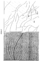
- Figure 9 shows how modelling of waveguide arrivals can be performed interactively on a computer workstation. The arrival times (left) for a user specified fault (right) can be superimposed on the data (left) for comparison with the times of observed arrivals.
- Synthetic seismograms corresponding to a set of line scatterers can also be generated (Figure 10).
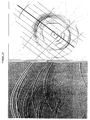
- Figure 10 shows how synthetic data (left) can be generated from a distribution of faults (the thin light lines on the right hand panel). These data can then be compared with the field data to evaluate the model of the fault distribution. Shown here are synthetic P-S arrivals and the direct arrival (Gaussian wavelet, centre frequency 18.75 Hz, 1/e half-width 12.5 Hz) for shotline 212 (bold). The truncation of arrivals is due to a upper limit imposed on the source offset from the coupling site. These data can also be migrated (right) to reveal the zones of illumination given by the survey as well as the extent of ambiguity of data that would be obtained from the survey. The amplitude of the coherent diffraction stack of the analytic signal is displayed here. Dark areas on the migration (right) show where coupling is likely to have occurred. Comparison of the synthetic seismograms with the field data evaluates the model.
- One migration method is the "diffraction" stack in which each point in the "migrated” image is calculated by a summation of all data samples that correspond to the travel time that would be associated with a scatterer at the point. For our survey technique this involves taking positions on the waveguide (usually a rectangular grid) and summing the values of the seismic traces at the travel times for a coupling segment at that point. For each point on the waveguide in turn, the waveguide travel time to the point is calculated. Then for each surface source the travel time from surface to the waveguide point is added to give a total travel time. The seismic trace samples corresponding to these total travel times for each of the sources are added to give the value of the migrated image. Values related to the probability of coupling having occurred are thus obtained at a set of points on the waveguide to give a migrated image of the waveguide. This is done for each component receiver gather.
- the diffraction stack is usually applied to the recorded signal. It is possible, however, to compute the "analytic" signal from a real seismic trace.
- the analytic signal has complex sample values whose real part is the recorded signal and whose imaginary part is the Hilbert Transform of the real part. If the magnitude of the complex number (analytic signal) is taken we get positive real numbers which form the "envelope" of the seismic trace. For a band limited transient pulse (the seismic pulse) the envelope of the trace falls off more slowly than the real signal as one moves away from the peak of the pulse. It also never changes sign, so cancellation (destructive interference) never occurs on the addition of more values.
- the envelope of the seismic trace is used in the diffraction stack (incoherent migration) instead of the real signal (coherent migration)
- the migrated image in the presence of random timing errors has a higher signal-to-noise ratio but lower resolution.
- signal-to-noise and resolution There is a trade-off between signal-to-noise and resolution.
- timing errors between our model of the velocity structure and reality
- Timing errors between our model of the velocity structure and reality
- a window of length equal to twice the effective correlation distance is run along the line.
- the coherent summation of the appropriate time samples is performed by adding the complex numbers (analytic signal).
- the amplitudes of these (complex) sums are then accumulated as the window runs along the line.
- the final accumulated value is the value of a "partial coherent" migration at that position on the waveguide.
- the coherent widow size is decided by a trade-off between resolution and signal-to-noise ratio.
- the chosen balance is a function of the timing error statistics (variance, correlation distance and degree of stationarity), the seismic wavelet shape (its dominant frequency, bandwidth) and the relative importance of resolution and signal-to-noise ratio to the geophysicist.
- Migration can be performed by extrapolating the recorded wavefield to the zone of interest and applying an imaging condition. Imaging can involve extracting the extrapolated received wavefield data at the time at which the source wavefield would have arrived (excitation-time imaging condition). Alternatively the extrapolated received wavefield is cross-correlated with the source wavefield. The source wavefield is obtained by extrapolating the seismic excitation out from the source position to the zone of interest. The latter is more robust with respect to noise but it does require knowledge of the source excitation.
- the adaptation necessary to migrate coupled waveguide modes involves using body wave extrapolation to model propagation from the surface to the waveguide and using a waveguide model for the propagation from coupling site to downhole geophone.
- Each component receiver gather can then be migrated by extrapolating the wavefield recorded at the (notional) surface array down to the waveguide.
- An imaging condition can then be applied to obtain the migrated image from the extrapolated traces.
- the value of the migrated image can be taken as the extrapolated data sample at the travel time for waveguide propagation.
- the source excitation is known imaging could be done by a cross-correlation of the extrapolated data with the source signature delayed by the waveguide travel time.
- the waveguide is dispersive (travel time changes with frequency), the dispersed nature of the arrivals on downward extrapolated data must be taken into account. Knowledge of the dispersion relation for the waveguide mode is necessary. Recompression of the downward extrapolated traces (based on their distance from the downhole geophone and the dispersion relation) would then allow application of a conventional excitation-time imaging condition.
- the dispersion could be modelled in the extrapolation of the (notional) source excitation out from the downhole position and a cross-correlation of the two wavefields would generate the migrated image.
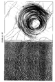
- Figure 11 illustrates partially coherent diffraction stack migration of the vertical component of Line 212 for P-S waveguide arrivals.
- the input data are displayed on the left and the migrated image on the right. Connections between features on the migration and the arrivals that generate them can be established by modelling.
- the letters A and B for example, mark interactively specified fault segments and their corresponding arrival times.
- the coherent window in the migration was 25 traces wide.
- Figure 12 illustrates partially coherent diffraction stack migration of the horizontal components of Line 212 for P-P waveguide arrivals. Both the horizontal components are used in the migration. For each possible coupling location the data is projected onto the expected polarization for an arrival from that direction.
- the migration will be dominated by the inline component close to the shotline whereas the parts of the image close to a line through the geophone and perpendicular to the shotline will be dominated by the crossline component.
- (a) we display the migrated image (right) with the inline component (left) when looking at features along the shotline (C, D and E) and in (b) we display the crossline component while investigating features off the shotline (F, G and H).
- the vertical component gather was used in the P-S migration since SV waveguide modes arriving at the downhole geophone would have a vertical polarisation.
- the P-P migrations used both the inline and crossline horizontal components in a projection onto the expected polarisation for an arrival from each waveguide position to get the signal.
- a partial coherent summation (25 trace window) of the analytic signal was performed to give the migrated value.
- the migrated images show coupling sites suggested by the data. Possible coupling sites can be compared with faults as mapped from the surface reflection data ( Figure 2). Correlation is good in several instances, despite the over-simplified model of the overburden that was used in the migrations.
- the modelling capabilities of the interactive program can establish relations between features on the migration and arrivals on the data.
- the coupled waveguide arrivals can be modelled by a linear system.
- S( ⁇ ) (S is complex and is the frequency) passes through the overburden as a body wave mode. This is more than a simple delay since attenuation effects and the lensing effects of propagating through a inhomogeneous overburden must be modelled.
- This filter can be modelled variously by a flat layered system, a 3-D inhomogeneous space under the ray (high frequency) approximation or a 3-D inhomogeneous space using wavefield propagators with various accuracies and ranges of applicability. For each source position, propagation through the overburden can be described by the transfer function H O ( ⁇ ) where H is complex.
- H W H W
- H C H C
- S source position
- H G can normally be reconstructed using the geophone tool manufacturer's specifications, the assumption that coupling to the borehole wall is firm and the orientation of the tool, leaving H W as the invariant part of R.
- S may be modelled using knowledge of the acquisition parameters and H O is obtained during the migration of the data. This leaves H C as the unknown and variable effect on R. If either H C or H W are known, the other can be solved for from R using Equation 2.
- H W may be modelled using knowledge of the velocity and density profiles of the waveguide (obtained from well-logs).
- the undispersed character of arrivals observed on the field data allowed us to make the assumption that the waveguide mode propagation velocity is independent of frequency (within the bandwidth of the data). This in turn suggests that the waveguide mode propagation velocity can be well approximated by the appropriate body wave mode (P or SV) propagation velocity along the axis of the low velocity layer. This velocity was inferred from the well-logs (sonic and density).
- Additional constraints can be inferred from analysis of migration focussing and the timing of P and S waveguide modes that have been scattered from the same coupling sites. If possible coupling sites are sparsely distributed, one can identify such corresponding arrivals. They have a common propagation time from surface source to waveguide, so the difference in arrival time can be attributed to the difference in their waveguide propagations velocities. If the position of the coupling sites is known, the arrival times would give the waveguide velocities directly. In practice, however, knowledge of the coupling site depends on knowledge of the waveguide velocities, so an iterative approach is used. The data will be migrated with different waveguide velocities until optimal focussing occurs.
- H W one can solve for the coupling transfer function H C from the data R on the basis of Equation 2.
- Inversion of H C for features of the departure from planarity is poorly constrained, but the use of additional knowledge allows inferences to be made.
- a geological model can provide a likely form for the features.
- the coupling sites are assumed to be steps in the roof of the waveguide caused by near vertical faults intersecting the base Zechstein/top Rotliengendes interface.
- Well-logs can provide reasonable values for the material properties.
- the salient feature in this model is the height of the step in the roof (throw of the fault).
- FIG. 13 is a map showing the survey layout (medium lines), the traces of faults in the Rotodes as mapped from surface seismic data (light lines) and the specular mode conversion sites responsible for the S arrivals to be examined (darkest lines).
- the specular mode conversion sites (or "illuminated segments" for P arrivals are slightly extended versions of those shown because of the higher post-conversion velocity.
- the specular mode conversion sites were modelled using the "Interactive Modeller" program on the assumption of a uniform image-ray travel time of 843ms and a constant normal moveout velocity of 3857m/s. These figures were obtained from the least-squares best fit of a hyperbolic sheet to all direct arrival travel times in the survey. Waveguide velocities of 3600m/s and 1800m/s were used for P and S arrivals respectively. Modelling identifies the faults responsible for particular arrivals.
- Corresponding P and S arrivals originate from the same site, except the specular P mode conversions take place along a greater length of the fault because of the higher post-scattering velocity.
- the two pairs of arrivals selected from Line 210 correlate with different segments of the same fault.
- the arrivals from Line 212 and Line 216 are modelled as coming from close but not coincident fault segments. There are no other prominent arrivals sufficiently close by to allow the problem to be resolved by changing the association of arrivals between lines.
- the arrivals can in fact be connected and thus identified as one and the same. The apparently different conversion sites for different parts of the same arrival suggests that distortion by the overburden has rendered the modelling procedure inaccurate.
- the faults in the region of the modelled mode conversion sites for Lines 212 and 216 have throws of about 30m.
- the fault corresponding to the mode conversion sites for Line 210 has a throw of 300m.
- the first trace of the KL transform (first PC) is a least-squares best fit trace to the gather traces, in which the freedom of scaling is permitted in the fits to each trace in the gather.
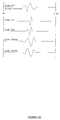
- Figure 14 shows the P-arrival signatures (extracted from the horizontal component receiver gathers) and
- Figure 15 shows the corresponding S-arrival signatures. Fairly narrow windows around the events were taken into the PCA in order to increase the signal-to-noise ratio.
- Figures 16 and 17 show the amplitude spectra. The direct arrival at the downhole geophone for a clean part of Line 212 is shown for the purposes of comparison for each of Figures 14 to 17.
- the arrival signatures can then be interpreted in terms of fault transfer functions H C ( ⁇ ).
- the fault transfer function is that which converts the incident P-wave I( ⁇ ) (direct arrival signature) into that which is recorded in the waveguide R( ⁇ ) (P and S-arrival signatures).
- H C ( ⁇ ) R( ⁇ )I*( ⁇ ) I( ⁇ )I*( ⁇ ) + ⁇
- the superscript * denotes the complex conjugate and (small and positive) represents white noise added to stabilise the calculation for frequency components that are very small in the autocorrelation of the input (I( ⁇ )I*( ⁇ )).
- the signatures were padded with zeros to improve sampling in the frequency domain and complex DFT of the signatures were performed.
- the resulting transfer functions are shown in the time domain in Figure 18 and in the frequency domain in Figure 19.
- the amplitude spectra show that (to first order) the small fault acts as a bandpass filter centred around 30 Hz while the large fault acts a bandpass filter centred on about 15 Hz.
Landscapes
- Engineering & Computer Science (AREA)
- Remote Sensing (AREA)
- Physics & Mathematics (AREA)
- Life Sciences & Earth Sciences (AREA)
- Acoustics & Sound (AREA)
- Environmental & Geological Engineering (AREA)
- Geology (AREA)
- General Life Sciences & Earth Sciences (AREA)
- General Physics & Mathematics (AREA)
- Geophysics (AREA)
- Geophysics And Detection Of Objects (AREA)
Applications Claiming Priority (2)
| Application Number | Priority Date | Filing Date | Title |
|---|---|---|---|
| GB9011836 | 1990-05-25 | ||
| GB909011836A GB9011836D0 (en) | 1990-05-25 | 1990-05-25 | Seismic surveying |
Publications (2)
| Publication Number | Publication Date |
|---|---|
| EP0481585A2 true EP0481585A2 (fr) | 1992-04-22 |
| EP0481585A3 EP0481585A3 (en) | 1992-08-12 |
Family
ID=10676630
Family Applications (1)
| Application Number | Title | Priority Date | Filing Date |
|---|---|---|---|
| EP19910304692 Withdrawn EP0481585A3 (en) | 1990-05-25 | 1991-05-23 | Seismic surveying |
Country Status (6)
| Country | Link |
|---|---|
| US (1) | US5260911A (fr) |
| EP (1) | EP0481585A3 (fr) |
| AU (2) | AU7735991A (fr) |
| CA (1) | CA2043249A1 (fr) |
| GB (1) | GB9011836D0 (fr) |
| ZA (2) | ZA912969B (fr) |
Families Citing this family (57)
| Publication number | Priority date | Publication date | Assignee | Title |
|---|---|---|---|---|
| RU2169931C2 (ru) * | 1996-04-12 | 2001-06-27 | Амоко Корпорейшн | Способ и устройство для обработки сейсмического сигнала и проведения разведки полезных ископаемых |
| US6108606A (en) * | 1996-09-17 | 2000-08-22 | Gas Research Institute | Waveguide disturbance detection method |
| US6147929A (en) * | 1998-03-03 | 2000-11-14 | Gas Research Institute | Method for predicting continuous and discontinuous waveguide targets using interwell seismic signature characteristics |
| AU6860201A (en) * | 2000-06-19 | 2002-01-02 | Halliburton Energy Serv Inc | Apparatus and methods for applying time lapse vsp to monitor a reservoir |
| GB2384557B (en) * | 2002-01-25 | 2005-06-29 | Westerngeco Ltd | A method of and apparatus for processing seismic data |
| US7480206B2 (en) * | 2004-09-13 | 2009-01-20 | Chevron U.S.A. Inc. | Methods for earth modeling and seismic imaging using interactive and selective updating |
| US7554883B2 (en) * | 2004-10-11 | 2009-06-30 | Landmark Graphics Corporation | Fault filter for seismic discontinuity data |
| ES2652413T3 (es) | 2006-09-28 | 2018-02-02 | Exxonmobil Upstream Research Company | Inversión iterativa de datos a partir de fuentes geofísicas simultáneas |
| US7545704B2 (en) * | 2007-02-13 | 2009-06-09 | Landmark Graphics Corporation | Performing 3-D scatterer imaging from 2-D seismic data |
| US8045417B2 (en) * | 2007-02-13 | 2011-10-25 | Landmark Graphics Corporation | Analyzing 2-D surface and/or borehole seismic data to locate subsurface diffractors |
| US9279899B2 (en) * | 2007-07-18 | 2016-03-08 | Westerngeco L.L.C. | System and technique to estimate physical propagation parameters associated with a seismic survey |
| US7900700B2 (en) * | 2007-08-02 | 2011-03-08 | Schlumberger Technology Corporation | Method and system for cleat characterization in coal bed methane wells for completion optimization |
| US7813218B2 (en) * | 2008-07-05 | 2010-10-12 | Westerngeco L.L.C. | Performing quality control with respect to positioning of survey hardware |
| US20100067328A1 (en) * | 2008-09-17 | 2010-03-18 | Andrew Curtis | Interferometric directional balancing |
| WO2010085493A1 (fr) * | 2009-01-20 | 2010-07-29 | Spectraseis Ag | Opérateurs d'imagerie par inversion dans le domaine temporel pour une localisation de source |
| US8542554B2 (en) * | 2009-11-10 | 2013-09-24 | Westerngeco L.L.C. | Method for velocity model building and analysis |
| US8537638B2 (en) | 2010-02-10 | 2013-09-17 | Exxonmobil Upstream Research Company | Methods for subsurface parameter estimation in full wavefield inversion and reverse-time migration |
| US8223587B2 (en) | 2010-03-29 | 2012-07-17 | Exxonmobil Upstream Research Company | Full wavefield inversion using time varying filters |
| US8694299B2 (en) | 2010-05-07 | 2014-04-08 | Exxonmobil Upstream Research Company | Artifact reduction in iterative inversion of geophysical data |
| US8756042B2 (en) | 2010-05-19 | 2014-06-17 | Exxonmobile Upstream Research Company | Method and system for checkpointing during simulations |
| US8767508B2 (en) | 2010-08-18 | 2014-07-01 | Exxonmobil Upstream Research Company | Using seismic P and S arrivals to determine shallow velocity structure |
| BR112013002842A2 (pt) | 2010-09-27 | 2016-06-07 | Exxonmobil Upstream Res Co | codificação de fonte e separação de fonte simultâneas como uma solução prática para inversão de campo de onda completa |
| US8437998B2 (en) | 2010-09-27 | 2013-05-07 | Exxonmobil Upstream Research Company | Hybrid method for full waveform inversion using simultaneous and sequential source method |
| SG189850A1 (en) | 2010-12-01 | 2013-06-28 | Exxonmobil Upstream Res Co | Simultaneous source inversion for marine streamer data with cross-correlation objective function |
| CN103703391B (zh) | 2011-03-30 | 2017-05-17 | 埃克森美孚上游研究公司 | 使用频谱整形的全波场反演的系统和计算机实施的方法 |
| CA2825469C (fr) | 2011-03-31 | 2017-06-13 | Exxonmobil Upstream Research Company | Procede d'estimation d'ondelettes et predictions multiples lors d'une inversion d'un champ d'ondelettes complet |
| ES2640824T3 (es) | 2011-09-02 | 2017-11-06 | Exxonmobil Upstream Research Company | Utilización de la proyección sobre conjuntos convexos para limitar la inversión del campo de onda completa |
| US9176930B2 (en) | 2011-11-29 | 2015-11-03 | Exxonmobil Upstream Research Company | Methods for approximating hessian times vector operation in full wavefield inversion |
| MY170622A (en) | 2012-03-08 | 2019-08-21 | Exxonmobil Upstream Res Co | Orthogonal source and receiver encoding |
| CN102914789B (zh) * | 2012-10-30 | 2015-07-29 | 中国石油化工股份有限公司 | 一种地震采集观测系统设置方法 |
| CA2892041C (fr) | 2012-11-28 | 2018-02-27 | Exxonmobil Upstream Research Company | Tomographie fondee sur le facteur de qualite q de donnees sismiques de reflexion |
| CN103235334B (zh) * | 2013-04-11 | 2015-06-10 | 中国矿业大学 | 基于地震信号的低抽巷道超前探测断层落差方法 |
| CA2909105C (fr) | 2013-05-24 | 2018-08-28 | Ke Wang | Inversion multiparametrique par fwi elastique dependante au decalage |
| US10459117B2 (en) | 2013-06-03 | 2019-10-29 | Exxonmobil Upstream Research Company | Extended subspace method for cross-talk mitigation in multi-parameter inversion |
| US9702998B2 (en) | 2013-07-08 | 2017-07-11 | Exxonmobil Upstream Research Company | Full-wavefield inversion of primaries and multiples in marine environment |
| DK3036566T3 (en) | 2013-08-23 | 2018-07-23 | Exxonmobil Upstream Res Co | SIMILAR SOURCE APPLICATION DURING BOTH SEISMIC COLLECTION AND SEISMIC INVERSION |
| US10036818B2 (en) | 2013-09-06 | 2018-07-31 | Exxonmobil Upstream Research Company | Accelerating full wavefield inversion with nonstationary point-spread functions |
| US9910189B2 (en) | 2014-04-09 | 2018-03-06 | Exxonmobil Upstream Research Company | Method for fast line search in frequency domain FWI |
| EP3140675A1 (fr) | 2014-05-09 | 2017-03-15 | Exxonmobil Upstream Research Company | Procédés efficaces de recherche du pas optimal pour inversion de champ d'ondes complet à paramètres multiples |
| US10185046B2 (en) | 2014-06-09 | 2019-01-22 | Exxonmobil Upstream Research Company | Method for temporal dispersion correction for seismic simulation, RTM and FWI |
| MX362753B (es) | 2014-06-17 | 2019-02-07 | Exxonmobil Upstream Res Co | Inversion rapida de campo de ondas completo viscoacustico y viscoelastico. |
| US10838092B2 (en) | 2014-07-24 | 2020-11-17 | Exxonmobil Upstream Research Company | Estimating multiple subsurface parameters by cascaded inversion of wavefield components |
| US10422899B2 (en) | 2014-07-30 | 2019-09-24 | Exxonmobil Upstream Research Company | Harmonic encoding for FWI |
| US10386511B2 (en) | 2014-10-03 | 2019-08-20 | Exxonmobil Upstream Research Company | Seismic survey design using full wavefield inversion |
| US9977141B2 (en) | 2014-10-20 | 2018-05-22 | Exxonmobil Upstream Research Company | Velocity tomography using property scans |
| US11163092B2 (en) | 2014-12-18 | 2021-11-02 | Exxonmobil Upstream Research Company | Scalable scheduling of parallel iterative seismic jobs |
| US10520618B2 (en) | 2015-02-04 | 2019-12-31 | ExxohnMobil Upstream Research Company | Poynting vector minimal reflection boundary conditions |
| EP3256886B1 (fr) | 2015-02-13 | 2020-01-29 | Exxonmobil Upstream Research Company | Condition de limite d'absorption efficace et stable dans des calculs à différence finie |
| AU2015383134B2 (en) | 2015-02-17 | 2018-01-25 | Exxonmobil Upstream Research Company | Multistage full wavefield inversion process that generates a multiple free data set |
| GB2554214A (en) * | 2015-05-22 | 2018-03-28 | Halliburton Energy Services Inc | In-situ borehole fluid speed and attenuation measurement in an ultrasonic scanning tool |
| US10416327B2 (en) | 2015-06-04 | 2019-09-17 | Exxonmobil Upstream Research Company | Method for generating multiple free seismic images |
| US10838093B2 (en) | 2015-07-02 | 2020-11-17 | Exxonmobil Upstream Research Company | Krylov-space-based quasi-newton preconditioner for full-wavefield inversion |
| RU2693495C1 (ru) | 2015-10-02 | 2019-07-03 | Эксонмобил Апстрим Рисерч Компани | Полная инверсия волнового поля с компенсацией показателя качества |
| US10520619B2 (en) | 2015-10-15 | 2019-12-31 | Exxonmobil Upstream Research Company | FWI model domain angle stacks with amplitude preservation |
| US10768324B2 (en) | 2016-05-19 | 2020-09-08 | Exxonmobil Upstream Research Company | Method to predict pore pressure and seal integrity using full wavefield inversion |
| CN106597540B (zh) * | 2016-12-30 | 2017-10-31 | 中国科学院地质与地球物理研究所 | 高斯束偏移成像方法及装置 |
| US11307317B2 (en) * | 2019-07-02 | 2022-04-19 | Saudi Arabian Oil Company | Systems and methods for data acquisition design of source and receiver locations |
Family Cites Families (12)
| Publication number | Priority date | Publication date | Assignee | Title |
|---|---|---|---|---|
| US2148422A (en) * | 1936-06-26 | 1939-02-28 | Standard Oil Dev Co | Method of determining the dips of geological strata with substantially vertical reflections |
| US2276335A (en) * | 1939-07-24 | 1942-03-17 | Cons Eng Corp | Method of making weathering corrections |
| US2718928A (en) * | 1951-03-07 | 1955-09-27 | Weiss Geophysical Corp | Seismic method of geological exploration |
| US2654874A (en) * | 1951-06-14 | 1953-10-06 | Socony Vacuum Oil Co Inc | Seismic exploration system |
| US2718929A (en) * | 1951-06-18 | 1955-09-27 | Weiss Geophysical Corp | Seismic method of geological exploration |
| CS150849B1 (fr) * | 1971-06-29 | 1973-09-17 | ||
| DE2345884C3 (de) * | 1973-09-12 | 1979-05-23 | Ruhrkohle Ag, 4300 Essen | Verfahren und Anordnung zur Vorfelderkundung im Zuge des Abbaus eines Kohleflözes |
| SU506817A1 (ru) * | 1974-03-27 | 1976-03-15 | Московский Геолого-Разведочный Институт Им. С.Орджоникидзе | Способ сейсморазведки |
| SU598003A1 (ru) * | 1976-06-01 | 1978-03-15 | Всесоюзный Научно-Исследовательский Институт Геофизических Методов Разведки | Способ сейсмической разведки |
| GB2032103B (en) * | 1978-10-20 | 1983-01-19 | Coal Industry Patents Ltd | Method and apparatus for locating flaws in a mineral seam |
| ZA806038B (en) * | 1979-10-19 | 1981-09-30 | Coal Ind | Method of stacking seismic data |
| US5005159A (en) * | 1989-11-01 | 1991-04-02 | Exxon Production Research Company | Continuity logging using differenced signal detection |
-
1990
- 1990-05-25 GB GB909011836A patent/GB9011836D0/en active Pending
-
1991
- 1991-05-23 EP EP19910304692 patent/EP0481585A3/en not_active Withdrawn
- 1991-05-24 CA CA002043249A patent/CA2043249A1/fr not_active Abandoned
- 1991-05-24 ZA ZA912969A patent/ZA912969B/xx unknown
- 1991-05-24 ZA ZA913969A patent/ZA913969B/xx unknown
- 1991-05-27 AU AU77359/91A patent/AU7735991A/en not_active Abandoned
- 1991-05-28 US US07/706,577 patent/US5260911A/en not_active Expired - Lifetime
-
1995
- 1995-03-23 AU AU15038/95A patent/AU675611B2/en not_active Ceased
Also Published As
| Publication number | Publication date |
|---|---|
| CA2043249A1 (fr) | 1991-11-26 |
| US5260911A (en) | 1993-11-09 |
| AU7735991A (en) | 1991-11-28 |
| GB9011836D0 (en) | 1990-07-18 |
| AU1503895A (en) | 1995-06-01 |
| AU675611B2 (en) | 1997-02-06 |
| ZA913969B (en) | 1993-03-24 |
| ZA912969B (en) | 1993-03-24 |
| EP0481585A3 (en) | 1992-08-12 |
Similar Documents
| Publication | Publication Date | Title |
|---|---|---|
| US5260911A (en) | Seismic surveying | |
| RU2319982C2 (ru) | Определение характеристик наклонных трещин с помощью обменных отраженных волн в сочетании с процессом последовательного исключения влияния вышележащих слоев | |
| US5671136A (en) | Process for seismic imaging measurement and evaluation of three-dimensional subterranean common-impedance objects | |
| EP0796441B1 (fr) | Procédé de traitement de signatures d'ondes de cisaillement réfléchies par les surfaces d'une formation géologique à anisotropie azimutale | |
| US5596548A (en) | Seismic imaging using wave equation extrapolation | |
| US6631783B2 (en) | Mapping reservoir characteristics using earth's nonlinearity as a seismic attribute | |
| AU2008216238B2 (en) | Performing 3-D scatterer imaging from 2-D seismic data | |
| Liu et al. | Fracture detection using crosshole surveys and reverse vertical seismic profiles at the Conoco Borehole Test Facility, Oklahoma | |
| EP2823337B1 (fr) | Extraction de données de cisaillement sv à partir de données marines d'onde p | |
| Oristaglio | A guide to current uses of vertical seismic profiles | |
| Aminzadeh et al. | Fundamentals of petroleum geophysics | |
| CA2485761C (fr) | Methode sismique de diffusion resonnante | |
| Lazaratos et al. | High-resolution, cross-well reflection imaging; Potential and technical difficulties | |
| US6678617B2 (en) | Mapping subsurface open fractures using elastically nonlinear interaction of two surface-generated waves | |
| Ahmed | Application of mode-converted shear waves to rock-property estimation from vertical seismic profiling data | |
| Lines et al. | Channel waves in cross-borehole data | |
| US20200209418A1 (en) | Method and Apparatus for Active Seismic Shear Wave Monitoring of Hydro-Fracturing of Oil and Gas Reservoirs Using Arrays of Multi-Component Sensors and Controlled Seismic Sources | |
| Peng et al. | Pressure in a fluid-filled borehole caused by a seismic source in stratified media | |
| MacBeth et al. | Examination of a Spectral Method for Measuring the Effects of ANISOTROPY1 | |
| Iverson | Crosswell logging for acoustic impedance | |
| Li et al. | Interpreting non‐orthogonal split shear waves for seismic anisotropy in multicomponent VSPS | |
| Hobbs et al. | 3D modeling of seismic-wave propagation using complex elastic screens, with application to mineral exploration | |
| O’Brien | VSP measurement of shear-wave velocities in consolidated and poorly consolidated formations | |
| Tang | Fracture hydraulic conductivity estimation from borehole Stoneley wave transmission and reflection data | |
| Gadallah et al. | Seismic Interpretation |
Legal Events
| Date | Code | Title | Description |
|---|---|---|---|
| PUAI | Public reference made under article 153(3) epc to a published international application that has entered the european phase |
Free format text: ORIGINAL CODE: 0009012 |
|
| AK | Designated contracting states |
Kind code of ref document: A2 Designated state(s): AT BE CH DE DK ES FR GB GR IT LI LU NL SE |
|
| PUAL | Search report despatched |
Free format text: ORIGINAL CODE: 0009013 |
|
| AK | Designated contracting states |
Kind code of ref document: A3 Designated state(s): AT BE CH DE DK ES FR GB GR IT LI LU NL SE |
|
| RIN1 | Information on inventor provided before grant (corrected) |
Inventor name: MCLAREN MASON,IAIN Inventor name: JACKSON,GEOFFREY MICHAEL Inventor name: CAMPBELL,DAVID STIRLING REDDICK Inventor name: LEE,DELMAN Inventor name: MOSHER,CHARLES CLINTON |
|
| 17P | Request for examination filed |
Effective date: 19941107 |
|
| 17Q | First examination report despatched |
Effective date: 19950609 |
|
| GRAG | Despatch of communication of intention to grant |
Free format text: ORIGINAL CODE: EPIDOS AGRA |
|
| GRAG | Despatch of communication of intention to grant |
Free format text: ORIGINAL CODE: EPIDOS AGRA |
|
| GRAH | Despatch of communication of intention to grant a patent |
Free format text: ORIGINAL CODE: EPIDOS IGRA |
|
| STAA | Information on the status of an ep patent application or granted ep patent |
Free format text: STATUS: THE APPLICATION IS DEEMED TO BE WITHDRAWN |
|
| 18D | Application deemed to be withdrawn |
Effective date: 19980829 |
|
| APAF | Appeal reference modified |
Free format text: ORIGINAL CODE: EPIDOSCREFNE |