EP0694862A2 - Reconnaissance de documents à niveaux de gris dégradés avec des pseudo-modèles de Markov cachés et à deux dimensions et avec des hypothèses de N meilleurs - Google Patents
Reconnaissance de documents à niveaux de gris dégradés avec des pseudo-modèles de Markov cachés et à deux dimensions et avec des hypothèses de N meilleurs Download PDFInfo
- Publication number
- EP0694862A2 EP0694862A2 EP95401397A EP95401397A EP0694862A2 EP 0694862 A2 EP0694862 A2 EP 0694862A2 EP 95401397 A EP95401397 A EP 95401397A EP 95401397 A EP95401397 A EP 95401397A EP 0694862 A2 EP0694862 A2 EP 0694862A2
- Authority
- EP
- European Patent Office
- Prior art keywords
- superstate
- path
- state
- gray
- level
- Prior art date
- Legal status (The legal status is an assumption and is not a legal conclusion. Google has not performed a legal analysis and makes no representation as to the accuracy of the status listed.)
- Withdrawn
Links
Images


Classifications
-
- G—PHYSICS
- G06—COMPUTING OR CALCULATING; COUNTING
- G06F—ELECTRIC DIGITAL DATA PROCESSING
- G06F18/00—Pattern recognition
- G06F18/20—Analysing
- G06F18/29—Graphical models, e.g. Bayesian networks
- G06F18/295—Markov models or related models, e.g. semi-Markov models; Markov random fields; Networks embedding Markov models
Definitions
- This invention relates to optical text recognition and more specifically to robust methods of recognizing characters or words regardless of impediments such as poor document reproduction.
- HMMs hidden Markov models
- OCR optical character recognition
- Optical recognition of text is often hampered by the use of characters with different sizes, blurred documents, distorted characters and other impediments. Accordingly, it is desirable to improve recognition methods to be robust regardless of such impediments.
- PHMMs Pseudo two-dimensional hidden Markov models
- Observation vectors for the gray-scale image are produced from pixel maps obtained by gray-scale optical scanning.
- Three components are employed to characterize a pixel: a convolved, quantized gray-level component, a pixel relative position component, and a pixel major stroke direction component. These components are organized as an observation vector, which is continuous in nature, invariant in different font sizes, and flexible for use in various quantization processes.
- the bi-level image may be compressed by subsampling into multi(gray)-level without losing information, thereby enabling recognition of the compressed images in a much shorter time.
- documents in gray-level may be scanned and processed with much lower resolution than in binary without sacrificing the performance. This significantly increases the processing speed.
- a character is represented by a pseudo two-dimensional HMM having a number of superstates, with each superstate having at least one state.
- the superstates represent vertical slices through the word image.
- Word images are compared with PHMMs by using a Viterbi algorithm incorporated in a level-building structure to calculate the probability that a particular PHMM represents a given section of the word image.
- Each possible model representation may be conceptualized as an hypothesis.
- An N-best hypothesis search is performed in combination with a duration constraint. Parameters for the models are generated by training routines.
- a technique termed the N-best hypotheses search may be advantageously utilized in conjunction with the approach developed above. This hypotheses search provides not only one, but N-best recognition hypotheses. By imposing postprocessing functions on these hypotheses, the recognition rate is greatly improved.
- the effectiveness of the aforementioned approaches is enhanced by employing duration constraints in the search processes.
- the word image to be recognized here in accordance with the invention will typically be part of a larger body of textual and graphical material on a page.
- the page has been optically scanned and that a word image to be recognized has been captured as a sequence of pixels generated by a conventional gray-level raster scan.
- Many techniques for performing such operations are well known to those skilled in the art. For example, see the articles "Global-to-local layout analysis” by H. Baird in the Proceedings of the LAPR Workshop on Syntactic and Structural Pattern Recognition, France, September 1988 and "Document Image Analysis" by S. Srihari and G. Zack in the Proceedings of the 8th International Conference on Pattern Recognition, Paris, October 1986.
- Such pixel sequences for known characters are used to "train" HMMs representing those characters.
- the pixel sequence for an unknown character string is then compared with the models to determine the probability that the models represent such unknown strings.
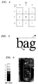
- FIG. 1 shows a pixel map 100 of the character "h” together with a corresponding state diagram 200 for a pseudo two-dimensional HMM for such character, in accordance with the invention.
- the model is termed a "top-down, left-right” model because it depicts the sequence of states resulting from a vertical gray-scale raster scan of the pixel map. It is called a "pseudo" two-dimensional model because it is not ergodic - that is, it is not a fully-connected two-dimensional network.
- superstates 210-214 Five “superstates” 210-214 are shown in state diagram 200. Such superstates correspond respectively to the five vertical regions 110-114 in pixel map 100. Note that all the columns of pixels in a given one of regions 110-114 are the same number of pixels. Within each superstate 210-214, the various vertical "states” possible in the columns of the corresponding region in the pixel map are shown. For example, superstate 211 includes three states 220-222 representing the white, black and white pixels respectively in the rows of region 111. However, it is to be understood that "white pixels” and “black pixels” are described for purposes of illustration. These pixels could represent any arbitrarily-selected gray level.
- Permitted transitions between superstates are denoted by arrows such as 230 and 231. Arrows such as 232 indicate that a transition can occur from a superstate to itself. Similarly, transitions between states are denoted by arrows such as 240 and 241 and transitions to the same state by arrows such as 242.
- An alternative to the structure of the model represented by state diagram 200 is a model using superstates representing horizontal slices.
- the sum of all the probabilities of transition from a state to another state or back to the same state must equal 1.
- a transition probability is associated with each transition from state 210 indicated by arrows 230, 231 and 232.
- the sum of the transition probabilities from a state to another state is the reciprocal of the duration of the state, measured in number of pixels.
- the length of a gray-level segment in a raster scan of the pixel map is represented by the associated transition probability; a long segment corresponds to a state with low transition probability to the next state; a short segment corresponds to a state with high transition probability.
- the same principles also apply to superstates.
- the presence of noise influences the probability of observing pixels having specific gray levels.
- the observations for a text element are based on the pixels.
- the of observation is based upon gray-level characterizations of pixels.
- Other kinds of observations can include additional information, such as transition or position information.
- each observation can be a vector quantity representing several different components. An example of such an observation vector will be given below.
- the pseudo two-dimensional hidden Markov model utilized by a preferred embodiment described herein employs a concept referred to as the duration probability of a character.
- D j s ⁇ D j 1
- the data structure used to represent a basic pseudo two- dimensional hidden Markov model consists of: the number of superstates (N v ), initial probabilities for the superstates (II v ), superstate transition probabilities (A v ), duration probabilities for character D(x), and, for each superstate: the number of states in the superstate (N h ), initial probabilities for the states (II h ), state transition probabilities within the superstate (A h ), duration probability for the superstate D i (x), observation probabilities for each state in the superstate (B h ); and, for each state, the duration probability D i j , for the state.
- An observation vector O xy may be defined for each pixel at coordinates (x, y).
- the observation vector O xy has three components.
- the first component of the observation vector, Osubbxy1 is calculated as: where m i,j is the gray-level of the pixel at (i, j), and c xy is from a 3 pixels by 3 pixels kernel as shown in FIG. 5.
- the kernel applies weighting factors to pixels as shown in FIG. 4.
- the kernel of FIG. 4 effectively convolves an entire image comprised of an array of pixels.
- the purpose of convolution is to reduce the effect of randomness on the grey level value caused by noise.
- the surrounding pixels are also contributing to the feature evaluation for the center pixel.
- the resulting gray level value of the pixel (from 0 to 255) is then quantized into 100 levels.
- the third component value of O xy is the direction of the major stroke in which the pixel resides.
- the entire image is subjected to a process of thresholding, described in greater detail in "minimum error thresholding", J. Kittler and J. Illingworth, Patent Recognition, Vol. 19, p. 41-47 (1986).
- the length of strokes (in terms of continuous black pixels) is computed in four directions: 0°, 45°, 90°, 135°, and the longest stroke is selected which passes the pixel as its major stroke direction.
- the 5th "direction" is for background pixels, which have no definition for direction or stroke.
- O xy thus has five distinct component values.
- Pseudo two-dimensional HMMs can be thought of as elastic templates because they allow for distortion in two dimensions, thus significantly increasing the robustness of the model. For example, vertical distortion, as often occurs in facsimile transmission, can be accommodated by the methods of the invention.
- the Viterbi algorithm is a well-known dynamic programming method that can be used for calculating the probability that a particular HMM is a match for a given sequence of observations.
- This algorithm is widely used in speech recognition as, for example, described in the article entitled "A tutorial on Hidden Markov Models and Selected Applications in Speech Recognition" by L. Rabiner in Proceedings of the IEEE, Vol. 77, pp.257-286, February 1989.
- the Viterbi algorithm has also been used in text recognition, as described in U. S. patent Application Serial No. 07/813,225 assigned to the assignee of the present patent application. mentioned above.
- the probability ⁇ of being in each state of the HMM is calculated for each observation, resulting in an N ⁇ T array, usually called a "trellis,” of probabilities where N is the number of states and T is the number of observations in the sequence.
- the highest such probability P* after the last observation in the sequence is used as the "score" for the HMM in regard to the sequence of observations.
- the process of tracking the sequence of states (and/or super-states) to determine the best path through the model is known as segmentation. For some applications an array of backpointers is also maintained so that the actual state sequence can be reconstructed.
- state as used herein throughout may refer to a state and/or a superstate.
- such state will be state N.
- the maximum probability after the last observation is associated with a state other than state N.
- the Viterbi algorithm is used repeatedly for the superstates and the states within each superstate.
- Such PHMMs are thus treated as nested one-dimensional models rather than truly two-dimensional.
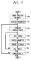
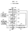
- FIG. 2 is a flow chart showing the operation of a computer programmed to compare a pixel map for a word image with a set of pseudo two-dimensional HMMs in accordance with the invention, in which the superstates represent vertical slices.
- Steps 300-307 show the main routine, which uses the Viterbi algorithm to calculate the maximum probability for segments of image from probabilities P* that a particular columns of pixels belongs in a particular superstate.
- Steps 301 and 304 of the main routine each use a subroutine, shown in steps 310-318, that uses the Viterbi algorithm for each superstate to calculate such probabilities P* for each column. It is assumed that the observations making up the pixel map and the various parameters for the HMMs are stored in appropriate memory areas in the computer performing the calculations.
- the observations for the first column are addressed (step 300). Then the subroutine (steps 310-318) is performed using such observations.
- T equals the number of observations
- a ij equals the transition probability from state i to state j.
- This equation extends the best paths through the states.
- the probability P* for such column and the current superstate is the last probability calculated for the final state in the column, not the maximum probability calculated after the last observation (step 316).
- step 317 An optional postprocessing step (step 317) is indicated, which can be used for various refinements to the method of the invention, as will be described below.
- step 318 If there are still more superstates (step 318), the state parameters of the next superstate are addressed (step 319) and steps 311-318 are repeated for the current column and the next superstate.
- the subroutine returns a probability P* for the current column and each superstate.
- the initial probabilities are calculated from the HMM superstate parameters ⁇ v and B v and equation (1) using such returned probabilities P* for observations O xy (step 302).
- the next column is addressed (step 303)
- the subroutine is repeated (step 304), and the best paths through the superstates are then extended by calculating the next set of superstate probabilities (step 305) using equation (3), the appropriate HMM parameters N v , A v and B v and the probabilities P* returned by the subroutine for observations O xy . If there are still more rows (step 306), steps 303, 304 and 305 are repeated for the next row.
- the ultimate likelihood score that the HMM represents the text element being compared is the last probability evaluated for the final superstate (step 307).
- an optional postprocessing step (step 308) is indicated for refinements to be explained. It will be clear that the above-described method can also be used for HMMs in which the superstates represent horizontal slices. In such cases, references to “columns" can be replaced with references to "rows”.
- the parameters ⁇ , A and B can be estimated for a pseudo two-dimensional HMM by using the segmental k-means algorithm described in the article entitled "A Segmental k-Means Training Procedure for Connected Word Recognition Based on Whole Word Reference Patterns” by L. Rabiner, J. Wilpon and B. Juang, AT&T Tech J., Vol. 65, pp. 21-36, May 1986.
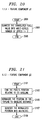
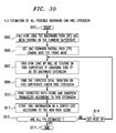
- FIG. 3 is a flowchart showing the procedure for creating a pseudo two-dimensional HMM. First, the structure of the model, that is, the number of superstates and states in each superstate, is determined (step 350).
- the two adjacent columns in region 112 each have two transitions and the same number of black and white pixels, corresponding to a superstate having three states.
- the column in region 113 also has two transitions, but with significantly different numbers of black and white pixels than the column in region 111, so the column in region 113 forms its own superstate.
- the number of superstates and states for each character model is determined by image topology. First, original columns are employed as initial blocks of the image, and then the two neighboring blocks which carry the highest cross correlation coefficient are grouped together to become one bigger block. This same grouping process is repeated until only a given number of blocks are left, or a certain correlation coefficient score threshold is reached. For example, the number of final blocks may be decided by inspecting character topology, and given before the grouping process starts. After those vertical blocks of columns are formed, one then examines each vertical block to group rows within the block by using the same process as was done for columns.
- FIG. 6 shows the final grouping (cutting) for image ⁇ b''.
- the character "b" can be represented by a PHMM with four superstates, and 3, 3, 5, 3 states within each superstate, respectively.
- the exact location as to where the cutting should be made is determined automatically through this iterated correlation comparison. This is specially important for gray-level images with noise and blur, for it is difficult to make meaningful, efficient, and consistent segmentation (grouping) for different characters and samples by manual operation.
- the procedure is repeated for a few sample images. Based on the segmentation, an initial estimate of the PHMM is constructed for the character. Note that this procedure is only required when there is no initial estimates of PHMMs available to start the training process.
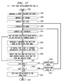
- the parameters for the model are initialized (step 351). This can be done by using parameters derived above from the sample used to create the structure. After the structure for the model is created and the parameters are initialized, the values of the parameters can be reestimated by "training" the model. Training may be accomplished using representative samples (tokens) of the word images in the form such images are likely to take in the text to be recognized (step 352). An observation sequence (pixel map) is created for each token, and the Viterbi algorithm is then used for segmentation of the observation sequence with respect to the model (step 353). The parameters are then updated in accordance with histograms of the results of the segmentation (step 354).
- ⁇ i number of tokens starting from state S i total number of tokens
- a ij number of transitions from state S i state S j total number of transitions starting from state S i
- b i (p) number of observations of p in state S i total number of observations
- the Viterbi algorithm is used to calculate a likelihood for each token with respect to the model, and such likelihoods for all tokens are combined (probabilities are multiplied, log probabilities are added) to provide an overall likelihood of the effectiveness of the model with respect to the tokens (step 355).
- the training procedure is complete (step 357). If not, the training procedure is repeated.
- a typical method of determining convergence is to compare the overall likelihoods from step 355 for successive iterations. If the difference is small, indicating that the parameters have not changed significantly during the last iteration, then convergence can be assumed.
- the parameters II h , A h and B h for the superstates and the parameters II v , A v and B v for the states within the superstates can all be determined by this method.
- P(d i ) a ii (d-1) a ij
- a ii the self-transition probability
- a ij is the transition probability to the next state.
- Segmentation into states is first accomplished using the parameters II, A and B as described above, then the scores calculated during segmentation are adjusted in a postprocessing step using the backpointers from array ⁇ to retrieve parameters for a more appropriate probability density for each state in the best path.
- An example of such adjustment is to replace the self-transition probabilities for each state with Gaussian state duration probability densities.
- the adjustment can be performed repeatedly on P* using the mean and standard deviation for each state passed through in turn. If P* is expressed as a logarithm, the adjustment can be accomplished by converting the adjustments to logarithmic form, summing such logarithmic adjustments for each state passed through and then adding the total adjustment to logP*.
- duration penalty is incorporated as part of the path search process, according to a preferred embodiment described herein.
- the duration probability may be found through training by calculating histogram of the length of the duration of states, superstates, and characters.
- the histogram for states is in units of pixels, and for superstates and characters are in columns.
- the duration penalty is added only when a transition occurs between different states, superstates or characters.
- the character duration penalty is added on top of the superstate duration penalty at the transition out of the last superstate of any character models. In this way, duration penalty is incorporated in the forward search, instead of as a postprocess.
- the incorporation of duration penalty greatly improves character recognition performance. Used in conjunction with an N-best approach, (to be described hereinafter) it can also give better word candidates, especially for those cases where the best candidate is not the correct one. It can also greatly reduce the search size for proper higher-level postprocessing (e.g. dictionary check).
- the best combination of character models can be identified by tracing back the optimal path.
- the corresponding word is the word recognized by the algorithm.
- the N-best hypotheses are obtained by first executing the nested Viterbi forward search, and then followed by a backward search.
- the backward search is worked around a main path stack, where each entry of the stack is a branch of the tree (a path), and is rank ordered from top down in the stack, according to its path likelihood score. It is understood that a back-tracing path should start from a terminal node. For each terminal node of each character model at every level, a null path is constructed with only a terminal node in it, along with its final accumulated path score obtained after the Viterbi search. The paths are inserted one by one in ranked order according to their path scores.
- the path score is still equal to the accumulated likelihood scores in the Viterbi search. No modification is performed yet. These paths will then develop backward towards their initial nodes (i.e. from right to left, towards frame 0).
- the paths are named the "backward partial paths” to identify the direction of path development, and to indicate that the backward development is not completed yet.
- the front-most node of this backward partial path i.e. the left most node of it, is here called “front node”.
- the backward development of the path is ⁇ completed'' when the front node is equal to the initial node. If M is the stack size, then after the top M null paths are placed into the stack, (those with top path scores out of all others), the initial stack setting up is finished.
- the process starts by removing the top path 1010 from the path stack 1000.
- This top path 1010 is the path which has the best path score among all paths for the time being. If the top path 1010 has already been subjected to the process described in this paragraph, put the top path 1010 back into the path stack 1000 and take the next path 1020 in the path stack 1000.
- the process described herein block 1050 is used to split the path into two separate paths: a first path 1080 with the best one arc (backward) extension and a second path 1090 with all remaining possible extensions.
- FIG. 8 is a small section of the path map obtained from forward Viterbi search, which is also used for backward tree search.
- Capital letters denote superstate nodes. When put as a string, they can also be used to represent a portion of a complete path. For example, ABCFG represents part of path 2 in FIG. 8.
- f x (y) represents the duration penalty for staying y units long in superstate x. The penalty is the minus of the log of duration probability.
- the growth of the backward path is constituted by sequential backward arc extension from terminal node T headed towards the initial node I. When doing the backward one-arc extension of the partial path, duration penalty is re-evaluated to reflect the exact duration fitness.
- a complete path here in CPS(E) is a connection of a backward Partial Path, formed by connected one-arc-extensions backward from the terminal node T all the way to node E (with score PPS(E)), and a Forward optimal Path from initial node I coming into E (with score FPS(E)).
- the forward optimal path is recorded during the forward trellis search.
- the path keeps record of the penalty it is paying for the current state.
- the penalty calculation is based on how long the path has been staying in this state, plus how long it will be staying before change to another state.
- the latter information is recorded as part of the best incoming path to each node in the forward search. Since the best incoming path might be different for each node, this penalty is updated together with other path information every time a backward one arc extension is made.
- DP should be f2(2), for staying over G, F in state 2. But when the path reaches node C, the ⁇ current state'' is now state 1, and the DP should now be updated as f1(3). This is from the expected traversal through C, B, and A, according to the path map.
- path ABCFG is preferred over path ADEFG in forward stage. This implies that, during the forward stage, the accumulated likelihood score at C should be better (smaller) than at E (so that F chose C at that time).
- path ABCFG was not compared with path ADEFG, but rather ABCF was compared with ADEF instead.
- the best path to G from F should be an extension of the best path into F. But this is not necessarily the case when duration penalty is added at the transition of each state. In the forward pass, it was not known how long the duration would be for the current state, until there is a change to another state.
- the duration penalty added in the complete path score is partly from the best forward path duration information, i.e. A-B-C for state 1 (implicitly as part of the score of the optimal forward path into F) and F-G for state 2 (explicitly recorded as DP in our backward path data). If, now at F, one tries to make an one-arc-extension backward, a comparison between F-C extension (path 2) and F-E extension (path 1) is necessary.
- This CDP information is calculated and stored in the node every time it is reached by a backward search path. Notice that CDPs of the same node could be different when reached by different backward search paths.
- the complete path score CPS is composed of the partial backward path score (PPS) and the score of the best incoming path into the front node, (FPS) which is the optimal forward partial path score recorded in forward Viterbi pass.
- the initial models for the training process were built from two images per character, with parameter (50, 0.8) and (20, 0.2), respectively.
- the k-mean training procedure can then operate on a larger training set to get the final converged models.
- the training set is generated in a similar manner as the training set for the initial models.
- the noise and blurring range are now (50 - 59, 0.8 - 0.7), with about 10 samples per character. Obviously, this is a training set with very narrow dynamic range. Nonetheless, this still results in a very robust models set, as will become evident from the experimental results.
- the size of each set is about 200 words, with more than 1,000 characters, and length varying from 2 to 12 characters.
- the first set is generated in the same parameter range as the training set.
- the second and third set is different from the first one, not only in term of blur and noise, or in the word collection in each set, but with the gap between characters in a word is now set to zero, instead of the original 1 pixel width in the training set and testing set 1. This results in images with connected neighboring character.
- the parameter range for set 2 is (70 - 79, 0.9 - 1.0), and set 3 is (80 - 89, 1.0 - 1.1).
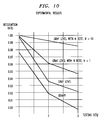
- the algorithms we compared are binary, gray-level, and gray-level with N-best search, all with duration constrain.
- N 1 case
- the experiment reveals to show the effectiveness of duration correcting in the backward search. Therefore, the recognized word is the word that comes out directly from the best in stack, right after the backward search with duration correction is completed. No postprocessing is imposed.
- the binary approach uses feature vectors with thresholded pixel value (0 or 1) as the first component to replace the gray-level one.
- the threshold algorithm used is the same algorithm used to extract the 3rd component of the feature vector, as described above.
- the rest of the vector components are exactly the same as the gray-level approach. This gives two approach a fair comparison.
- duration correction By incorporating duration penalty first in forward Viterbi search and then backward, duration correction could eliminate hypotheses with unreasonable matching. This way only the more plausible words, i.e., words with similar number of characters and/or similar topology, would be found. This is especially important when working on poorly-printed document images.
- a PHMM can be completely specified by a set of parameters with the following description. For the clearness of the expression, we omit the model index here, with an understanding that different PHMM will have the same set of parameters with different values.
- the observation vector O xy for each pixel located at (x, y) has three components:
- the first component of the observation vector, O 1 xy is calculated as: where m i,j is the gray-level of the pixel at (i, j), c xy is from a 3 pixels by 3 pixels kernel.
- the weightings of the kernel were shown in Fig. 4. In another words, we use this kernel to convolve with the whole image.
- the purpose is to reduce the effect of randomness on the grey level value caused by noise.
- the surrounding pixels are also contributing to the feature evaluation for the center pixel.
- the resulting gray level value of the pixel (from 0 to 255) is then quantized into 100 levels.
- the second component is the relative position of each pixel in the columns.
- the third component value is the direction of the major stroke in which the pixel resides.
- We threshold the whole image the threshold algorithm is explained in the experimental setup.
- Fig 12 shows three paths among others obtained after a completed Viterbi search with PHMM.
- This Viterbi search is performed between a complete word image (with N frames/columns) and a PHMM with four superstates. Each path represents a possible match between the model and the image. If we assume that b j (O i ) is the likelihood that observation of column i is generated by superstate j, and a kl is the superstate transition probability from superstate k to 1, then the likelihood of path A should be: in -log() scale b0(O0)+a02+b2(O 1) +a22+b2(O 2) +a23 +b3(O3)+a33+b3(O4)+a33+b3(O 5) + ... +a33+b3(O N-1)
- b2(O 1) b 0 2 (O 10) +a 00 2 +b 0 2 (O 11) +a 00 2 +b 0 2 (O12)+a 01 2 +b 1 2 (O 13) +a 11 2 +b 1 2 (O 14) +...+b 2 2 (O 1, M-1) where M is the total number of pixels in one column.
- M the total number of pixels in one column.
- the former is the likelihood of a column generated by the 1D HMM in a superstate. This likelihood is different from column to column, infinite in the number of possible values; the latter is the likelihood of a pixel generated by one state, which is finite in the discrete observation case, and could be in parametric form in continuous case through training. Thus, the latter is part of the model parameter, and the former is not (at least in practical sense).
- This nested Viterbi algorithm is a crucial part of the training and recognition process.
- a nested Viterbi algorithm for PHMM is the major one dimensional Viterbi search, from left to right, column by column, to find the best match between the word image and models; where between each column of the image and each superstate of each model, another one dimensional Viterbi search is engaged, from top to bottom, pixel by pixel, to find the best match between pixels and states within each column.
- This nested structure is clearly shown in Fig. 12, where the upper part is the main Viterbi search between the image and PHMM, and the lower part shows where does the 1D search fit in.
- the Viterbi search progresses from left to right, until the last frame is finished. The overall likelihood of the image being generated by the PHMM is obtained.
- a word image has to be matched with all possible combinations of PHMMs from all characters.
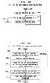
- FIG. 13 is an extension of Fig. 12 by adding one more dimension for accommodating all possible character models, and building levels to search for the optimal model combination.
- An outlet point of model "a" at frame 4 is concatenated by another match of model "a" at level 2, from frame 5 and up. This path then represents a possible recognition of character "a” from frame 0 up to 4 and then another "a” from frame 5 and up.
- the rule for selecting an outlet to continue the path is:
- s m is the last superstate of model m
- M is the total number of models in this case.
- the duration probability is found through training by calculating histogram of the length of the duration of states, superstates, and characters.
- the histogram for states is in units of pixels, and for superstates and characters are in columns.
- the duration penalty is added only when a transition occurs between different states, superstates or characters.
- the character duration penalty is added on top of the superstate duration penalty at the transition out of the last superstate of any character models. In this way, duration penalty could be incorporated in the forward search, instead of as a postprocess.
- An initial node is just the opposite: it is the first node (superstate) at the first frame of the observation for a path. Obviously, if we trace back a path starting from a terminal node, it will end up at the initial node. Assume we have found the terminal node of the optimal path, then we need to know what is the previous node right before the current node if tracing backward along this optimal path. What level, model, and superstate does this previous node belong to? If the back-tracing is for training, we need to know exactly where does each model, superstate, state start and end, with precise pixel and column index, plus all the observation vectors generated by each state. Only in this way can we have all the information needed to update our models.
- the main purpose of back-tracing is to get frame by frame recovery of the optimal path in the superstate level, plus a pixel by pixel recovery of the optimal path in state level within each node of the superstate level optimal path.
- the basic information we need from this process is the link information from the current node (superstate or state) to one node before along the optimal path. The exact usage of the information obtained in this process for training and recognition will be discussed in detail in the following sections.
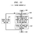
- the summary of this back-tracing within a level-building structure is as follows (FIG.
- the optimal path will show: a) at superstate level, where are the boundaries (in terms of column index) of each superstate and character. b) at state level, where are the boundaries (in terms of pixel index) of each state.
- the information is retrieved by back-tracing this optimal path in both superstate and state level. Once this segmentation information is obtained, we will be able to know exactly which model, superstate, and state does each pixel belong to. We then group pixel observation vectors according to this information.
- D(n) the number of training tokens of this character that have duration of n columns the number of training tokens of this character
- a kj the number of transition from superstate k to superstate j the number of all transitions start from superstate k
- D j (n) the number of tokens of superstate j that has duration of n columns the number of tokens of superstate j
- im j (p) the number of vectors for state s 1 j which have observation p in the mth vector component the number of vectors in state s 1 j
- D 1 j (n) the number of tokens of state
- the final step in the training loop is the test for convergence as a criterion to stop the iteration.
- Fig. 6 shows the final grouping (cutting) for image ⁇ b''.
- the character ⁇ b'' can be represented by a PHMM with four superstates, and 3, 3, 5, 3 states within each superstate, respectively. The exact location as to where the cutting should be made is determined automatically through this iterated correlation comparison.
- the performance can be further improved by incorporating discriminative training.
- discriminative training When checking the wrongly-recognized words in the experiment, almost all of these words are clustered in a so-called ⁇ confusion set''. That is, characters are mistaken for other ones with similar topology, and these characters got more confusing when images were noisy and blurry.
- discriminative training is used to train the models with this competitive set, it could greatly reduce the error rate of recognition. This motivation could be confirmed by the N-best hypotheses approach results.
- Most of the words found in the hypotheses list i.e. those that are considered top competitive to the correct one, are mostly combination of characters from the confusion set.
- the utilization of gray-scale imaging in combination with pseudo 2-dimensional Markov modeling provides significant improvement over binary systems, especially for degraded and connected word images.
- An N-best hypotheses search with duration constrain is introduced to further improve the system.
- the duration constraint is first imposed in the forward Viterbi search as added penalty, then is combined with the path map obtained in the forward pass to do the duration penalty correction in the backward search.
- Experimental results have proven the superiority of the system in the form of greatly improved recognition rate, and robustness over widely changed applications.
Landscapes
- Engineering & Computer Science (AREA)
- Data Mining & Analysis (AREA)
- Theoretical Computer Science (AREA)
- Computer Vision & Pattern Recognition (AREA)
- Bioinformatics & Cheminformatics (AREA)
- Bioinformatics & Computational Biology (AREA)
- Artificial Intelligence (AREA)
- Evolutionary Biology (AREA)
- Evolutionary Computation (AREA)
- Physics & Mathematics (AREA)
- General Engineering & Computer Science (AREA)
- General Physics & Mathematics (AREA)
- Life Sciences & Earth Sciences (AREA)
- Character Discrimination (AREA)
- Image Analysis (AREA)
Applications Claiming Priority (2)
| Application Number | Priority Date | Filing Date | Title |
|---|---|---|---|
| US27873394A | 1994-07-22 | 1994-07-22 | |
| US278733 | 1994-07-22 |
Publications (2)
| Publication Number | Publication Date |
|---|---|
| EP0694862A2 true EP0694862A2 (fr) | 1996-01-31 |
| EP0694862A3 EP0694862A3 (fr) | 1996-07-24 |
Family
ID=23066128
Family Applications (1)
| Application Number | Title | Priority Date | Filing Date |
|---|---|---|---|
| EP95401397A Withdrawn EP0694862A3 (fr) | 1994-07-22 | 1995-06-15 | Reconnaissance de documents à niveaux de gris dégradés avec des pseudo-modèles de Markov cachés et à deux dimensions et avec des hypothèses de N meilleurs |
Country Status (3)
| Country | Link |
|---|---|
| US (1) | US5754695A (fr) |
| EP (1) | EP0694862A3 (fr) |
| JP (1) | JPH0877301A (fr) |
Cited By (1)
| Publication number | Priority date | Publication date | Assignee | Title |
|---|---|---|---|---|
| WO1999065225A1 (fr) * | 1998-06-12 | 1999-12-16 | At & T Corp. | Systeme ameliorant la qualite d'un document envoye par telecopie |
Families Citing this family (28)
| Publication number | Priority date | Publication date | Assignee | Title |
|---|---|---|---|---|
| JPH1011434A (ja) * | 1996-06-21 | 1998-01-16 | Nec Corp | 情報認識装置 |
| US6137863A (en) * | 1996-12-13 | 2000-10-24 | At&T Corp. | Statistical database correction of alphanumeric account numbers for speech recognition and touch-tone recognition |
| US6154579A (en) * | 1997-08-11 | 2000-11-28 | At&T Corp. | Confusion matrix based method and system for correcting misrecognized words appearing in documents generated by an optical character recognition technique |
| US6219453B1 (en) | 1997-08-11 | 2001-04-17 | At&T Corp. | Method and apparatus for performing an automatic correction of misrecognized words produced by an optical character recognition technique by using a Hidden Markov Model based algorithm |
| US6141661A (en) * | 1997-10-17 | 2000-10-31 | At&T Corp | Method and apparatus for performing a grammar-pruning operation |
| US6122612A (en) * | 1997-11-20 | 2000-09-19 | At&T Corp | Check-sum based method and apparatus for performing speech recognition |
| US6205428B1 (en) | 1997-11-20 | 2001-03-20 | At&T Corp. | Confusion set-base method and apparatus for pruning a predetermined arrangement of indexed identifiers |
| US6223158B1 (en) | 1998-02-04 | 2001-04-24 | At&T Corporation | Statistical option generator for alpha-numeric pre-database speech recognition correction |
| US6205261B1 (en) * | 1998-02-05 | 2001-03-20 | At&T Corp. | Confusion set based method and system for correcting misrecognized words appearing in documents generated by an optical character recognition technique |
| EP0961218B1 (fr) * | 1998-05-28 | 2004-03-24 | International Business Machines Corporation | Procédé de binarisation dans un système de reconnaissance de caractères |
| US7937260B1 (en) | 1998-06-15 | 2011-05-03 | At&T Intellectual Property Ii, L.P. | Concise dynamic grammars using N-best selection |
| US6400805B1 (en) | 1998-06-15 | 2002-06-04 | At&T Corp. | Statistical database correction of alphanumeric identifiers for speech recognition and touch-tone recognition |
| US6757449B1 (en) * | 1999-11-17 | 2004-06-29 | Xerox Corporation | Methods and systems for processing anti-aliased images |
| JP2001266142A (ja) * | 2000-01-13 | 2001-09-28 | Nikon Corp | データ分類方法及びデータ分類装置、信号処理方法及び信号処理装置、位置検出方法及び位置検出装置、画像処理方法及び画像処理装置、露光方法及び露光装置、並びにデバイス製造方法 |
| US6947179B2 (en) * | 2000-12-28 | 2005-09-20 | Pitney Bowes Inc. | Method for determining the information capacity of a paper channel and for designing or selecting a set of bitmaps representative of symbols to be printed on said channel |
| US7274800B2 (en) * | 2001-07-18 | 2007-09-25 | Intel Corporation | Dynamic gesture recognition from stereo sequences |
| US7209883B2 (en) * | 2002-05-09 | 2007-04-24 | Intel Corporation | Factorial hidden markov model for audiovisual speech recognition |
| US20030212552A1 (en) * | 2002-05-09 | 2003-11-13 | Liang Lu Hong | Face recognition procedure useful for audiovisual speech recognition |
| US7165029B2 (en) | 2002-05-09 | 2007-01-16 | Intel Corporation | Coupled hidden Markov model for audiovisual speech recognition |
| JP2004078631A (ja) * | 2002-08-20 | 2004-03-11 | Fujitsu Ltd | オブジェクト指向データベースにおける検索装置及び検索方法 |
| US7171043B2 (en) * | 2002-10-11 | 2007-01-30 | Intel Corporation | Image recognition using hidden markov models and coupled hidden markov models |
| US7472063B2 (en) * | 2002-12-19 | 2008-12-30 | Intel Corporation | Audio-visual feature fusion and support vector machine useful for continuous speech recognition |
| US7203368B2 (en) * | 2003-01-06 | 2007-04-10 | Intel Corporation | Embedded bayesian network for pattern recognition |
| US7623725B2 (en) * | 2005-10-14 | 2009-11-24 | Hewlett-Packard Development Company, L.P. | Method and system for denoising pairs of mutually interfering signals |
| FR2892847B1 (fr) * | 2005-11-03 | 2007-12-21 | St Microelectronics Sa | Procede de memorisation de donnees dans un circuit de memoire pour automate de reconnaissance de caracteres de type aho-corasick et citcuit de memorisation correspondant. |
| US7587308B2 (en) * | 2005-11-21 | 2009-09-08 | Hewlett-Packard Development Company, L.P. | Word recognition using ontologies |
| US8554825B2 (en) | 2005-12-22 | 2013-10-08 | Telcordia Technologies, Inc. | Method for systematic modeling and evaluation of application flows |
| US8290273B2 (en) * | 2009-03-27 | 2012-10-16 | Raytheon Bbn Technologies Corp. | Multi-frame videotext recognition |
Family Cites Families (9)
| Publication number | Priority date | Publication date | Assignee | Title |
|---|---|---|---|---|
| US4177448A (en) * | 1978-06-26 | 1979-12-04 | International Business Machines Corporation | Character recognition system and method multi-bit curve vector processing |
| US5261009A (en) * | 1985-10-15 | 1993-11-09 | Palantir Corporation | Means for resolving ambiguities in text passed upon character context |
| JPS63225300A (ja) * | 1987-03-16 | 1988-09-20 | 株式会社東芝 | パタ−ン認識装置 |
| US5075896A (en) * | 1989-10-25 | 1991-12-24 | Xerox Corporation | Character and phoneme recognition based on probability clustering |
| JPH0833739B2 (ja) * | 1990-09-13 | 1996-03-29 | 三菱電機株式会社 | パターン表現モデル学習装置 |
| US5321773A (en) * | 1991-12-10 | 1994-06-14 | Xerox Corporation | Image recognition method using finite state networks |
| US5438630A (en) * | 1992-12-17 | 1995-08-01 | Xerox Corporation | Word spotting in bitmap images using word bounding boxes and hidden Markov models |
| KR950013127B1 (ko) * | 1993-03-15 | 1995-10-25 | 김진형 | 영어 문자 인식 방법 및 시스템 |
| US5699456A (en) * | 1994-01-21 | 1997-12-16 | Lucent Technologies Inc. | Large vocabulary connected speech recognition system and method of language representation using evolutional grammar to represent context free grammars |
-
1995
- 1995-06-15 EP EP95401397A patent/EP0694862A3/fr not_active Withdrawn
- 1995-07-21 JP JP7185551A patent/JPH0877301A/ja not_active Withdrawn
-
1996
- 1996-10-16 US US08/734,369 patent/US5754695A/en not_active Expired - Lifetime
Non-Patent Citations (3)
| Title |
|---|
| CVGIP GRAPHICAL MODELS AND IMAGE PROCESSING, vol. 57, no. 2, 1 March 1995, pages 131-145, XP000546687 CHINCHING YEN ET AL: "DEGRADED GRAY-SCALE TEXT RECOGNITION USING PSEUDO-2D HIDDEN MARKOV MODELS AND N-BEST HYPOTHESES" * |
| ICASSP 91. 1991 INTERNATIONAL CONFERENCE ON ACOUSTICS, SPEECH AND SIGNAL PROCESSING (CAT. NO.91CH2977-7), TORONTO, ONT., CANADA, 14-17 MAY 1991, ISBN 0-7803-0003-3, 1991, NEW YORK, NY, USA, IEEE, USA, pages 705-708 vol.1, XP002002818 SOONG F K ET AL: "A tree-trellis based fast search for finding the N-best sentence hypotheses in continuous speech recognition" * |
| IMAGE AND MULTIDIMENSIONAL SIGNAL PROCESSING, MINNEAPOLIS, APR. 27 - 30, 1993, vol. 5 OF 5, 27 April 1993, INSTITUTE OF ELECTRICAL AND ELECTRONICS ENGINEERS, pages V-113-V-116, XP000437631 AGAZZI O E ET AL: "CONNECTED AND DEGRADED TEXT RECOGNITION USING PLANAR HIDDEN MARKOV MODELS" * |
Cited By (1)
| Publication number | Priority date | Publication date | Assignee | Title |
|---|---|---|---|---|
| WO1999065225A1 (fr) * | 1998-06-12 | 1999-12-16 | At & T Corp. | Systeme ameliorant la qualite d'un document envoye par telecopie |
Also Published As
| Publication number | Publication date |
|---|---|
| US5754695A (en) | 1998-05-19 |
| EP0694862A3 (fr) | 1996-07-24 |
| JPH0877301A (ja) | 1996-03-22 |
Similar Documents
| Publication | Publication Date | Title |
|---|---|---|
| US5754695A (en) | Degraded gray-scale document recognition using pseudo two-dimensional hidden Markov models and N-best hypotheses | |
| Kuo et al. | Keyword spotting in poorly printed documents using pseudo 2-D hidden Markov models | |
| EP0605099B1 (fr) | Reconnaissance de texte utilisant des modèles stochastiques bi-dimensionnels | |
| CN111931736B (zh) | 利用非自回归模型与整合放电技术的唇语识别方法、系统 | |
| US8005294B2 (en) | Cursive character handwriting recognition system and method | |
| Agazzi et al. | Hidden Markov model based optical character recognition in the presence of deterministic transformations | |
| El-Hajj et al. | Arabic handwriting recognition using baseline dependant features and hidden Markov modeling | |
| Kim et al. | A lexicon driven approach to handwritten word recognition for real-time applications | |
| JP3056905B2 (ja) | 文字認識方法およびテキスト認識システム | |
| CA2171773C (fr) | Construction automatique de gabarits de caractere au moyen d'une transcription et d'un modele de source d'images bidimensionnelles | |
| US7480408B2 (en) | Degraded dictionary generation method and apparatus | |
| Agazzi et al. | Connected and degraded text recognition using planar hidden Markov models | |
| Hu et al. | Comparison and classification of documents based on layout similarity | |
| CN111401099B (zh) | 文本识别方法、装置以及存储介质 | |
| EP0097820B1 (fr) | Procédé pour l'adjonction adaptable des numéros d'index aux éléments d'image des dessins de matrice | |
| Lu et al. | Robust language-independent OCR system | |
| KR19990010210A (ko) | 대용량 패턴 정합 장치 및 방법 | |
| Kuo et al. | Machine vision for keyword spotting using pseudo 2D hidden Markov models | |
| CN115862045A (zh) | 基于图文识别技术的病例自动识别方法、系统、设备及存储介质 | |
| CN118038052A (zh) | 一种基于多模态扩散模型的抗差异医学图像分割方法 | |
| Amara et al. | Printed PAW recognition based on planar hidden Markov models | |
| Yen et al. | Degraded gray-scale text recognition using pseudo-2D hidden Markov models and N-best hypotheses | |
| Yen et al. | Degraded documents recognition using pseudo 2-D hidden Markov models in gray-scale images | |
| Liang et al. | Segmentation of handwritten interference marks using multiple directional stroke planes and reformalized morphological approach | |
| CN119919789B (zh) | 一种水下珊瑚礁生态多样化识别方法及系统 |
Legal Events
| Date | Code | Title | Description |
|---|---|---|---|
| PUAI | Public reference made under article 153(3) epc to a published international application that has entered the european phase |
Free format text: ORIGINAL CODE: 0009012 |
|
| AK | Designated contracting states |
Kind code of ref document: A2 Designated state(s): FR |
|
| PUAL | Search report despatched |
Free format text: ORIGINAL CODE: 0009013 |
|
| AK | Designated contracting states |
Kind code of ref document: A3 Designated state(s): FR |
|
| 17P | Request for examination filed |
Effective date: 19960819 |
|
| STAA | Information on the status of an ep patent application or granted ep patent |
Free format text: STATUS: THE APPLICATION IS DEEMED TO BE WITHDRAWN |
|
| 18D | Application deemed to be withdrawn |
Effective date: 19990105 |