EP0886837B1 - Estimation d'erreur de champ de vecteur de mouvement - Google Patents
Estimation d'erreur de champ de vecteur de mouvement Download PDFInfo
- Publication number
- EP0886837B1 EP0886837B1 EP97908166A EP97908166A EP0886837B1 EP 0886837 B1 EP0886837 B1 EP 0886837B1 EP 97908166 A EP97908166 A EP 97908166A EP 97908166 A EP97908166 A EP 97908166A EP 0886837 B1 EP0886837 B1 EP 0886837B1
- Authority
- EP
- European Patent Office
- Prior art keywords
- error
- motion vector
- motion
- video
- matrix
- Prior art date
- Legal status (The legal status is an assumption and is not a legal conclusion. Google has not performed a legal analysis and makes no representation as to the accuracy of the status listed.)
- Expired - Lifetime
Links
Images





Classifications
-
- H—ELECTRICITY
- H04—ELECTRIC COMMUNICATION TECHNIQUE
- H04N—PICTORIAL COMMUNICATION, e.g. TELEVISION
- H04N19/00—Methods or arrangements for coding, decoding, compressing or decompressing digital video signals
- H04N19/50—Methods or arrangements for coding, decoding, compressing or decompressing digital video signals using predictive coding
- H04N19/503—Methods or arrangements for coding, decoding, compressing or decompressing digital video signals using predictive coding involving temporal prediction
- H04N19/51—Motion estimation or motion compensation
-
- G—PHYSICS
- G06—COMPUTING OR CALCULATING; COUNTING
- G06T—IMAGE DATA PROCESSING OR GENERATION, IN GENERAL
- G06T7/00—Image analysis
- G06T7/20—Analysis of motion
- G06T7/269—Analysis of motion using gradient-based methods
-
- H—ELECTRICITY
- H04—ELECTRIC COMMUNICATION TECHNIQUE
- H04N—PICTORIAL COMMUNICATION, e.g. TELEVISION
- H04N5/00—Details of television systems
- H04N5/14—Picture signal circuitry for video frequency region
- H04N5/144—Movement detection
- H04N5/145—Movement estimation
Definitions
- the invention relates motion estimation in video and film signal processing, in particular, to a technique for assessing the reliability of motion vectors.
- Gradient motion estimation is one of three or four fundamental motion estimation techniques and is well known in the literature (references 1 to 18). More correctly called 'constraint equation based motion estimation' it is based on a partial differential equation which relates the spatial and temporal image gradients to motion.
- Gradient motion estimation is based on the constraint equation relating the image gradients to motion.
- Prefiltering can be applied to the image sequence to avoid the problem of direct measurement of the image gradients. If spatial low pass filtering is applied to the sequence then the effective size of 'pixels' is increased. The brightness gradients at a particular spatial location are then related for a wider range of motion speeds. Hence spatial low pass filtering allows higher velocities to be measured, the highest measurable velocity being determined by the degree of filtering applied. Vertical low pass filtering also alleviates the problem of vertical aliasing caused by interlace. Alias components in the image tend to be more prevalent at higher frequencies. Hence, on average, low pass filtering disproportionately removes alias rather than true signal components. The more vertical filtering that is applied the less is the effect of aliasing.
- One advantage of this invention is its ability to detect erroneous motion estimates due to vertical aliasing.
- Prefiltering an image sequence results in blurring. Hence small details in the image become lost. This has two consequences, firstly the velocity estimate becomes less accurate since there is less detail in the picture and secondly small objects cannot be seen in the prefiltered signal.
- hierarchical techniques are sometimes used. This involves first calculating an initial, low accuracy, motion vector using heavy prefiltering, then refining this estimate to higher accuracy using less prefiltering. This does, indeed, improve vector accuracy but it does not overcome the other disadvantage of prefiltering, that is, that small objects cannot be seen in the prefiltered signal, hence their velocity cannot be measured. No amount of subsequent vector refinement, using hierarchical techniques, will recover the motion of small objects if they are not measured in the first stage. Prefiltering is only advisable in gradient motion estimation when it is only intended to provide low accuracy motion vectors of large objects.
- each pixel in the image gives rise to a separate linear equation relating the horizontal and vertical components of the motion vector and the image gradients.
- the image gradients for a single pixel do not provide enough information to determine the motion vector for that pixel.
- the gradients for at least two pixels are required. In order to minimise errors in estimating the motion vector it is better to use more than two pixels and find the vector which best fits the data from multiple pixels.
- Each pixel restricts the motion vector to a line in velocity space. With two pixels a single, unique, motion vector is determined by the intersection of the 2 lines. With 3 pixels there are 3 lines and, possibly, no unique solution. This is illustrated in figure 1.
- the vectors E 1 to E 3 are the error from the best fitting vector to the constraint line for each pixel.
- Equation 3 The least mean square solution for a group of neighbouring pixels is given by the solution of Equation 3; where where (u 0 , v 0 ) is the best fit motion vector and the summations are over a suitable region.
- Equation 4 The (direct) solution of equation 3 is given by Equation 4; Analysing small image regions produces detailed vector fields of low accuracy and vice versa for large regions. There is little point in choosing a region which is smaller than the size of the prefilter since the pixels within such a small region are not independent.
- motion estimators generate motion vectors on the same standard as the input image sequence.
- motion compensated standards converters or other systems performing motion compensated temporal interpolation, it is desirable to generate motion vectors on the output image sequence standard.
- the input image sequence is 625 line 50Hz (interlaced) and the output standard is 525 line 60Hz (interlaced).
- a motion compensated standards converter operating on a European input is required to produce motion vectors on the American output television standard.
- the matrix in equation 3 (henceforth denoted 'M') may be analysed in terms of its eigenvectors and eigenvalues. There are 2 eigenvectors, one of which points parallel to the predominant edge in the analysis region and the other points normal to that edge. Each eigenvector has an associated eigenvalue which indicates how sharp the image is in the direction of the eigenvector.
- the eigenvectors and values are defined by Equation 5;
- the eigenvectors e i are conventionally defined as having length 1, which convention is adhered to herein.
- the eigenvectors In plain areas of the image the eigenvectors have essentially random direction (there are no edges) and both eigenvalues are very small (there is no detail). In these circumstances the only sensible vector to assume is zero. In parts of the image which contain only an edge feature the eigenvectors point normal to the edge and parallel to the edge. The eigenvalue corresponding to the normal eigenvector is (relatively) large and the other eigenvalue small. In this circumstance only the motion vector normal to the edge can be measured. In other circumstances, in detailed parts of the image where more information is available, the motion vector may be calculated using Equation 4.
- the motion vector may be found, taking into account Martinez' ideas above, by using Equation 6; where superscript t represents the transpose operation.
- n 1 & n 2 are the computational or signal noise involved in calculating ⁇ 1 & ⁇ 2 respectively.
- n 1 ⁇ n 2 both being determined by, and approximately equal to, the noise in the coefficients of M.
- ⁇ 1 & ⁇ 2 «n the calculated motion vector is zero; as is appropriate for a plain region of the image.
- ⁇ 1 »n and ⁇ 2 «n then the calculated motion vector is normal to the predominant edge in that part of the image.
- equation 6 becomes equivalent to equation 4.
- equation 6 provides an increasingly more accurate estimate of the motion vectors as would be expected intuitively.
- FIG. 2 A block diagram of a direct implementation of gradient motion estimation is shown in figures 2 & 3.
- the apparatus shown schematically in Figure 2 performs filtering and calculation of gradient products and their summations.
- the apparatus of Figure 3 generates motion vectors from the sums of gradient products produced by the apparatus of figure 2.
- the horizontal (10) and vertical (12) low pass filters in figure 2 perform spatial prefiltering as discussed above.
- the cut-off frequencies of 1/32nd band horizontally and 1/16th band vertically allow motion speeds up to (at least) 32 pixels per field to be measured. Different cut-off frequencies could be used if a different range of speeds is required.
- the image gradients are calculated by three temporal and spatial differentiating filters (16,17,18).
- the vertical/temporal interpolation filters (20) convert the image gradients, measured on the input standard, to the output standard.
- the vertical/temporal interpolators (20) are bilinear interpolators or other polyphase linear interpolators.
- the interpolation filters are a novel feature (subject of GB-A-2311183) which facilitates interfacing the motion estimator to a motion compensated temporal interpolator.
- Temporal low pass filtering is normally performed as part of (all 3 of) the interpolation filters.
- the temporal filter (14) has been re-positioned in the processing path so that only one rather than three filters are required. Note that the filters prior (10,12,14) to the multiplier array can be implemented in any order because they are linear filters.
- the summation of gradient products, specified in equation 3, are implemented by the low pass filters (24) following the multiplier array.
- these filters (24) would be (spatial) running average filters, which give equal weight to each tap within their region of support. Other lowpass filters could also be used at the expense of more complex hardware.
- the size of these filters (24) determines the size of the neighbourhood used to calculate the best fitting motion vector. Examples of filter coefficients which may be used can be found in the example.
- FIG. 4 A block diagram of apparatus capable of implementing equation 6 and which replaces that of figure 3, is shown in figures 4 and 5.
- Each of the 'eigen analysis' blocks (30), in figure 4, performs the analysis for one of the two eigenvectors.
- These 's' vectors are combined with vector ( ⁇ xt 2 , ⁇ yt 2 ) (denoted c in figure 4), according to equation 6, to give the motion vector according to the Martinez technique.
- the eigen analysis illustrated in figure 5, has been carefully structured so that it can be implemented using lookup tables with no more than 2 inputs. This has been done since lookup tables with 3 or more inputs would be impracticably large using today's technology.
- the implementation of figure 5 is based on first normalising the matrix M by dividing all its elements by ( ⁇ xx 2 + ⁇ yy 2 ). This yields a new matrix, N, with the same eigenvectors (e 1 & e 2 ) and different (but related) eigenvalues (X 1 & X 2 ).
- Equation 7 The relationship between M, N and their eigenvectors and values is given by Equation 7; Matrix N is simpler than M as it contains only two independent values, since the principle diagonal elements (N 1,1, N 2,2 ) sum to unity and the minor diagonal elements (N 1,2 , N 2,1 ) are identical.
- the principal diagonal elements may be coded as ( ⁇ xx 2 - ⁇ yy 2 )/( ⁇ xx 2 + ⁇ yy 2 ) since Equation 8;
- lookup tables 1 & 2 have all the information they require to find the eigenvalues and vectors of N using standard techniques. It is therefore straightforward to precalculate the contents of these lookup tables.
- Lookup table 3 simply implements the square root function. The key features of the apparatus shown in figure 5 are that the eigenanalysis is performed on the normalised matrix, N , using 2 input lookup tables (1 & 2) and the eigenvalue analysis (from table 2) is rescaled to the correct value using the output of table 3.
- the gradient motion estimator described above is undesirably complex.
- the motion estimator is robust to images containing limited information but figures 4 and 5 show the considerable complexity involved. The situation is made worse by the fact that many of the signals have a very wide dynamic range making the functional blocks illustrated much more difficult to implement.
- Equation 9 Dividing the constraint equation by the modulus of the gradient vector yields a normalised constraint equation i.e. Equation 9:
- Equation 10 Equation 10
- ⁇ is the angle between the spatial image gradient vector ( ⁇ I) and the horizontal
- vn is the motion speed in the direction of the image gradient vector, that is, normal to the predominant edge in the picture at that point.
- the coefficients of equation 10 (cos( ⁇ ) & sin( ⁇ )) have a well defined range (0 to 1) and, approximately the same dynamic range as the input signal (typically 8 bits).
- vn has a maximum (sensible) value determined by the desired motion vector measurement range. Values of vn greater than the maximum measurement range, which could result from either noise or 'cuts' in the input picture sequence, can reasonably be clipped to the maximum sensible motion speed.
- the apparatus of figure 6 performs the calculation of the normalised constraint equation (equation 10) for each pixel or data value. Obviously, if prefiltering is performed the number of independent pixel values is reduced, the effective pixel size is greater.
- the filtering in figure 6 is identical to that in figure 2.
- the spatial image gradients converted to the output standard are used as inputs for a rectangular to polar co-ordinate converter (32) which calculates the magnitude of the spatial image vector and the angle ⁇ .
- a suitable converter can be obtained from Raytheon (Co-ordinate transformer, model TMC 2330).
- a lookup table (34) is used to avoid division by very small numbers when there is no detail in a region of the input image.
- the constant term, 'n', used in the lookup table is the measurement noise in estimating
- a limiter (36) has also been introduced to restrict the normal velocity, vn, to its expected range (determined by the spatial prefilter). The normal velocity might, otherwise, exceed its expected range when the constraint equation is violated, for example at picture cuts.
- a key feature of figure 6 is that, due to the normalisation that has been performed, the two outputs, vn & ⁇ , have a much smaller dynamic range than the three image gradients in figure 2, thereby allowing a reduction in the hardware complexity.
- the input video is first filtered using separate temporal, vertical and horizontal filters (10,12,14), the image gradients are calculated using three differentiating filters (16,18) and then converted, from the input lattice, to the output sampling lattice using three vertical/temporal interpolators (20), typically bilinear or other polyphase linear filters.
- the image gradients might be calculated on a 525/60/2:1 lattice.
- the parameters of the normalised constraint equation, vn & ⁇ are calculated as shown.
- the apparatus of figure 7 calculates the best fitting motion vector, corresponding to a region of the input image, from the constraint equations for the pixels in that region.
- the summations specified in equation 12 are implemented by the lowpass filters (38) following the polar to rectangular co-ordinate converter (40) and lookup tables 5 & 6.
- these filters (38) would be (spatial) running average filters, which give equal weight to each tap within their region of support. Other lowpass filters could also be used at the expense of more complex hardware.
- the size of these filters (38) determine the size of the neighbourhood used to calculate the best fitting motion vector.
- Lookup tables 5 & 6 are simply cosine and sine lookup tables.
- Lookup tables 7 to 9 contain precalculated values of matrix 'Z' defined by Equation 14; where e and ⁇ are the eigenvectors and eigenvalues of ⁇ . Alternatively Z could be ⁇ -1 (i.e. assuming no noise), but this would not apply the Martinez technique and would give inferior results.
- a key feature of figure 7 is that the elements of matrix Z are derived using 2 input lookup tables. Their inputs are the output from the two lowpass filters (39) which have a small dynamic range allowing the use of small lookup tables.
- US-A-4838685 discloses a method of estimating motion vectors from images by generating motion vectors for regions of an input signal involving calculating a plurality of spatial and temporal image gradients for each region.
- the motion vector is calculated by a least mean squares fitting process.
- This method is based on the use of the constraint equation and hence is particularly suitable for use with gradient based motion estimation techniques as described above.
- the method is more general than this and could also be used to estimate the accuracy of motion vectors measured in other ways, for example, using a block matching technique.
- the measurement of the accuracy of motion vectors is a new technique.
- Most of the literature on motion estimation concentrates almost wholly on ways of determining the 'best' motion vector and pays scant regard to considering whether the resulting motion vectors are actually accurate. This may, in part, explain why motion compensated processing is, typically, unreliable for certain types of input image.
- the invention provides video or film signal processing apparatus comprising motion estimation apparatus for generating motion vectors each corresponding to a region of an input signal, logic means adapted to calculate, for each motion vector, an estimate of the length and orientation of the axes of the error distribution in measuring said motion vector, and means adapted to generate, for each said vector, an indication of the motion vector measurement error derived from said estimate.
- the logic means may provide, for each vector, a statistical analysis of the error in the constraint equation for each of a plurality of pixels in a region of the input signal.
- the logic means may provide, for each motion vector, a matrix representing the dimensions and orientation of the error distribution.
- the apparatus may include means for calculating an error value for each of a plurality of pixels in a region of the input signal based on the normalised constraint equation for each pixel, and means for calculating a plurality of corresponding error vectors.
- the apparatus may include means for calculating the elements of an error matrix from said error vectors, said matrix representing the distribution of motion vector measurement errors.
- the apparatus may include means for calculating the standard deviation of the error in the constraint equations for each of a plurality of pixels in a region of said input signal, and means for estimating the error in measuring the motion vector using the resultant standard deviation, whereby an estimate of the autocovariance matrix for the measured motion vector is generated.
- the apparatus may further include means for performing an eigenvector analysis on said error matrix or on said covariance matrix.
- the invention also provides a method of video or film signal processing comprising generating motion vectors each corresponding to a region of an input signal, calculating for each motion vector an estimate of the length and orientation of the axes of the error distribution in measuring said motion vector, and generating, for each said vector, an indication of the motion vector measurement error derived from said estimate.
- Figure 1 shows graphically the image gradient constraint lines for three pixels.
- Figures 2 and 3 are a block diagram of a motion estimator.
- Figures 4 is a block diagram of apparatus for calculating motion vectors which can be substituted for the apparatus of fig. 3.
- Figure 5 is a block diagram of apparatus for implementing the eigen analysis required in figure 4.
- Figures 6 and 7 show another example of a motion estimation apparatus.
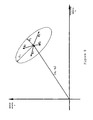
- Figure 8 shows graphically the distribution of errors in the case of a best fit motion vector.
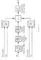
- Figure 9 is a block diagram of apparatus for calculating the elements of an error matrix.
- Figure 10 is a block diagram for calculating a scalar error factor.
- Figure 11 is a block diagram for calculating the elements of a covariance matrix.
- Figure 12 is an apparatus according to the invention for generating error values in the form of spread vectors and a scalar measurement of the error.
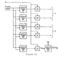
- Figure 13 is another embodiment of apparatus according to the invention which can be substituted for the apparatus of figures 11 and 12.
- the set of error vectors, ⁇ E i ⁇ form a two dimensional distribution of errors in motion vector space, illustrated in figure 8.
- This distribution of motion vector measurement errors would be expected to be a two dimensional Gaussian (or Normal) distribution.
- the distribution occupies an elliptical region around the true motion vector.
- the ellipse defines the area in which most of the estimates of the motion vector would lie; the 'best' motion vector points to the centre of the ellipse.
- Figure 8 illustrates the 'best' motion vector, (u 0 , v 0 ), and 4 typical error vectors, E 1 to E 4 .
- Equation 18 The matrix (E t .E)/N (henceforth the 'error matrix' and denoted Q for brevity) can be expanded to give Equation 19; where the summation is over a region of the image containing N pixels.
- the elements of the error matrix may be calculated by the apparatus of figure 9. Other implementations are possible, but figure 9 is straight forward and efficient.
- the inputs to figure 9, ⁇ and vn, may be derived as in figure 6.
- the motion vector input to figure 9, (u, v), could be derived as in figure 7, however it could equally well come from any other source such as figure 3 or 4 or even a block matching motion estimator.
- the lookup tables (10 and 11) are simply cosine and sine tables and, as in figures 2 & 7, the required summations are performed using spatial lowpass filters (42) such as running average filters.
- the error matrix can give a good indication of the vector error, for some types of picture it may be misleading. Misleading results, using the error matrix, may occur in parts of the picture which contain predominantly an edge feature. With this type of picture the error matrix gives an underestimate of the vector error parallel to the edge. That is the error matrix is a biased measure of the vector error under these circumstances.
- the reason for this bias can be understood by considering a set of nearly parallel constraint lines (as specified in equations 2, 9 or 10 and illustrated in figure 1). With nearly parallel constraint lines the error vectors (defined in equation 16) will be nearly perpendicular to the constraint lines and hence perpendicular to the edge feature in the image. In these circumstance the major error in the estimate of the motion vector will be parallel to the edge. However the error vectors will have a small component in this direction, hence underestimating the true error in this direction.
- An alternative measure of the error in the motion vector can be derived using the techniques of linear regression analysis (described in reference 19 and elsewhere).
- regression analysis it is assumed that a random (zero mean) error term, with known standard deviation is added to each constraint equation. Knowing the error added to each constraint equation the techniques of linear algebra can be applied to calculate the cumulative effect of the errors, in all the constraint equations, on the final motion vector estimate.
- a priori the standard deviation of the error in the constraint equations. However this can be estimated once the best fitting motion vector has been estimated. Measuring the error in the motion vector, using this technique, is thus a three stage process. First estimate the best fitting motion vector. Then estimate the standard deviation of the error in the constraint equations. Then use this standard deviation to estimate the error in the best fitting motion vector.
- a covariance matrix is a well known multidimensional analogue of the variance of a 1 dimensional random variable.
- Equation 20 has a scalar and a matrix factor which expand as;
- S the scalar error factor
- Cov the covariance matrix
- Q ( E t . E )/N, defined in equation 19.
- Equation 21 is seemingly complicated the covariance matrix Cov is easily derived from intermediate results already calculated to estimate the motion vector.
- the scalar error factor, S can be calculated by the apparatus of figure 10, whilst ⁇ t . ⁇ (as described in equation 8) has already been calculated to estimate the motion vector.
- Note the inputs to figure 10 have been generated as shown in figures 6 or 7; ⁇ vn.cos( ⁇ ) and ⁇ vn.sin( ⁇ ) being taken after the spatial interpolators if these are included in the system.
- the complete covariance matrix, Cov may be calculated by the apparatus of figure 11.
- the lookup tables in figure 11 each calculate one of the 3 different components of the matrix inverse of ⁇ t . ⁇ .
- the two inputs to these lookup tables completely specify ⁇ t . ⁇ as described in equations 11 and 12, hence the content of these lookup tables may easily be precalculated.
- the vector error distribution is described by a matrix because the motion vector is, obviously, a vector rather than a scalar quantity.
- the covariance matrix is the multidimensional analogue of the variance of a scalar quantity.
- Matrices Q and Cov are simply different descriptions of the error distribution.
- For a scalar variable there are also alternative measures of the error such as the standard deviation (root mean square error) or the mean absolute error.
- the error or covariance matrix contains all the information about the error distribution it is sometimes convenient to derive alternative descriptions of the distribution.
- One convenient representation involves analysing the error or covariance matrix in terms of its eigenvectors and eigenvalues.
- the error distribution may be thought of as an elliptical region round the motion vector (figure 8).
- the eigenvectors describe the orientation of the principle axes of the ellipse and the eigenvalues their radii.
- the eigenvalues are the variance, ⁇ 2 , in the direction of their corresponding eigenvector.
- the error or covariance matrix has been calculated (e.g. as in figure 9 or 10 and 11) its eigenvalues and eigenvectors may be found using the implementation of figure 12 whose inputs are the elements of the error or covariance matrix, i.e. ⁇ (error 2 .cos 2 ( ⁇ )), ⁇ (error 2 .cos( ⁇ ).sin( ⁇ )) and ⁇ (error 2 .sin 2 ( ⁇ )) or Cov 1,1 , Cov 1,2 and Cov 2,2 , denoted Q 11 , Q 12 and Q 22 respectively.
- the implementation of figure 12 since there are two eigenvalues the implementation of figure 12 must be duplicated to generate both eigenvectors.
- figure 12 As in figure 5, described previously, the implementation of figure 12 has been carefully structured so that it uses look up tables with no more than 2 inputs.
- the output of lookup table 15 is the angular orientation of an eigenvector, that is the orientation of one of the principle axes of the (2 dimensional) error distribution.
- the output of lookup table 16, once it has been rescaled by the output of lookup table 17, is proportional to the square root of the corresponding eigenvalue.
- An alternative function of the eigenvalue may be used depending on the application of the motion vector error information.
- the motion vector measurement errors may not have a Gaussian distribution but the spread vectors, defined above, still provide a useful measure of the error distribution.
- An alternative, simplified, output of figure 12 is a scalar confidence signal rather than the spread vectors. This may be more convenient for some applications.
- a signal may be derived from, r error , the product of the outputs of lookup tables 17 and 18 in figure 12, which provides a scalar indication of the motion vector measurement error.
- the scalar error is the geometric mean of the standard deviation along the principle axes of the error distribution. That is it is the 'radius' of a circular, i.e. isotropic error distribution with the same area as the (anisotropic)elliptical distribution.
- the confidence signal may then be used to implement graceful fallback in a motion compensated image interpolator as described in reference 4.
- the motion vector may be scaled by the confidence signal so that it remains unchanged for small motion vector errors but tends to zero for large errors as the confidence decreases to zero.
- the r error signal is a scalar, average, measure of motion vector error. It assumes that the error distribution is isotropic and, whilst this may not be justified in some situations, it allows a simple confidence measure to be generated. Note that the scalar vector error, r error , is an objective function, of the video signal, whilst the derived confidence signal is an interpretation of it.
- a confidence signal may be generated by assuming that there is a small range of vectors which shall be treated as correct. This predefined range of correct vectors will depend on the application. We may, for example, define motion vectors to be correct if they are within, say, 10% of the true motion vector. Outside the range of correct vectors we shall have decreasing confidence in the motion vector.
- the parameters k and r 0 can be adjusted during testing to achieve best results.
- the region of confidence is proportional to the measured motion speed accept at low speeds when it is a small constant.
- the confidence value is then calculated, for each output motion vector, as the probability that the actual velocity is within the confidence radius, r confident , of the measured velocity. This may be determined by assuming a Gaussian probability distribution: giving the following expression for vector confidence (equation 24):
- FIG. 6 An embodiment of apparatus for estimating vector error is shown in figures 6, 7, 9 and 12, or in figure 6, 7, 10, 11 and 12.
- the apparatus of figure 9 calculates the error matrix using the outputs from the apparatus of figure 6, which were generated previously to estimate the motion vector.
- the apparatus of figures 10 and 11 calculates the covariance matrix using output from the apparatus of figures 6 and 7, which were generated previously to estimate the motion vector.
- the error matrix, ( E t . E )/N, or covariance matrix, Cov input in figure 12 is denoted Q to simplify the labelling.
- lookup table 17 in figure 12 is a dimensioned parameter (z) which describes the scale of the distribution of motion vector errors.
- the content of lookup table 17 is defined by ⁇ z.
- the output of Lookup table 17 is a scaling factor which can be used to scale the output of lookup table 16 defined above.
- the input to the polar to rectangular co-ordinate converter is, therefore, related to the length of each principle axis of the error distribution. Using a different lookup table it would be possible to calculate the spread vectors directly in Cartesian coordinates.
- the apparatus described in relation to figure 12, is capable of producing both the spread vectors and the scalar confidence signal.
- the present invention also encompasses methods and apparatus which generate only one such parameter; either the confidence signal or the spread vectors.
- the eigen analyses performed by the apparatus of figure 12 must be performed twice to give both spread vectors for each principle axis of the error distribution; only one implementation of figure 12 is required to generate r error and the derived confidence signal.
- the inputs to lookup table 18 are the same as for lookup table 15 (x and y).
- the content of Lookup table 18 is defined by 4 ⁇ (1 ⁇ 4(1-x 2 )-y 2 ).
- r error a scalar (isotropic) vector error from which a confidence signal is generated in lookup table 19, the contents of which are defined by equation 24, for example.
- FIG. 6 An alternative embodiment of apparatus for estimating motion vector error is shown in figures 6, 7, 10 and 13. This embodiment may be used if the error is estimated using the covariance matrix but not using the error matrix.
- a key feature of this embodiment is that many functions of the covariance matrix may be generated using only a 2 input lookup table and multiplier as shown in figure 13.
- the apparatus of figure 13 calculates the spread vectors and r error using intermediate signals from figure 7, ⁇ cos(2 ⁇ ) and ⁇ sin(2 ⁇ ) (taken after the spatial interpolators if these are included in the system), which were generated previously to estimate the motion vector, and the scalar error factor, S, which is the output of figure 10.
- the top 4 lookup tables of figure 13 each generate a component of one of the 2 vectors defined in equation 25. Since the inputs to the lookup tables completely define ⁇ t . ⁇ (as noted above) it is straight forward to precalculate the content of these lookup tables. Multiplied by the scalar error factor, S, the vector components defined in equation 25 give the components of the two spread vectors defined above (identical to the spread vector outputs of figure 12). Hence the outputs of the top 4 multipliers each produce one component (horizontal or vertical) of one of the two spread vectors (defined above).
- Lookup table 24 and the bottom multiplier of figure 13 generate r error (identical to r error of figure 12) which is then combined with the motion speed in lookup table 25 to give the confidence signal (identical to that in figure 12).
- Lookup table 24 generates the square root of the determinant of ( ⁇ t . ⁇ ) -1 which when multiplied by S gives r error .
- the output of lookup table 24 is given by equation 26.
- Lookup table 25 in figure 13 has exactly the same function and content as lookup table 19 in figure 12.
- picture resizing is allowed for using (intrafield) spatial interpolators (44) following the region averaging filters (38,39,42). Picture resizing is optional and is required for example for overscan and aspect ratio conversion.
- the apparatus of figure 6 generates its outputs on the nominal output standard, that is assuming no picture resizing.
- the conversion from input to (nominal) output standard is achieved using (bilinear) vertical/temporal interpolators(20).
- these interpolators (20) could also perform the picture stretching or shrinking required for resizing.
- the region averaging filters (38,42) in figures 7, 9 and 10 would have to vary in size with the resizing factor.
- This example provides a brief specification for a gradient motion estimator for use in a motion compensated standards converter.
- the input for this gradient motion estimator is interlaced video in either 625/50/2:1 or 525/60/2:1 format.
- the motion estimator produces motion vectors on one of the two possible input standards and also an indication of the vector's accuracy on the same standard as the output motion vectors.
- the motion vector range is at least ⁇ 32 pixels/field.
- the vector accuracy is output as both a 'spread vector' and a 'confidence signal'.
- a gradient motion estimator is shown in block diagram form in figures 6 & 7 above. Determination of the measurement error, indicated by 'spread vectors' and 'confidence' are shown in figures 9 & 12.
- the characteristics of the functional blocks of these block diagrams is as follows: Input Video: 4:2:2 raster scanned interlaced video. luminance component only Active field 720 pixel ⁇ 288 or 244 field lines depending on input standard. Luminance coding 10 bit, unsigned binary representing the range 0 to (2 10 -1)
- Temporal Halfband Lowpass Filter (14) Function: Temporal filter operating on luminance. Implemented as a vertical/temporal filter because the input is interlaced. The coefficients are defined by the following matrix in which columns represent fields and rows represent picture (not field) lines. Input:10 bit unsigned binary representing the range 0 to 1023 (decimal). Output:12 bit unsigned binary representing the range 0 to 1023.75(decimal) with 2 fractional bits.
- Vertical Lowpass Filter Function: Vertical intra field, 1/16 th band, lowpass, prefilter and anti-alias filter. Cascade of 3, vertical running sum filters with lengths 16, 12 and 5 field lines. The output of this cascade of running sums is divided by 1024 to give an overall DC gain of 15/16. The overall length of the filter is 31 field lines. Input: As Temporal Halfband Lowpass Filter output. Output: As Temporal Halfband Lowpass Filter output.
- Horizontal Lowpass Filter Function: Horizontal, 1/32 nd band, lowpass, prefilter. Cascade of 3, horizontal, running sum filters with lengths 32, 21 and 12 pixels. The output of this cascade is divided by 8192 to give an overall DC gain of 63/64. The overall length of the filter is 63 pixels. Input: As Vertical Lowpass Filter output. Output: As Vertical Lowpass Filter output.
- Input As Horizontal Lowpass Filter output.
- Output 12 bit 2's complement binary representing the range -2 9 to (+2 9 - 2 -2 ).
- Horizontal Differentiator (17) Function: Horizontal differentiation of prefiltered luminance signal. 3 tap horizontal filter with coefficients 1 ⁇ 2(1, 0,-1) on consecutive pixels. Input: As Horizontal Lowpass Filter output. Output: 8 bit 2's complement binary representing the range -2 4 to (+2 4 - 2 -3 ).
- Compensating Delay Function: Delay of 1 input field. Input & Output: As Horizontal Lowpass Filter output.
- Vertical/Temporal Interpolators Function: Conversion between input and output scanning standards. Cascade of intra field, 2 field line linear interpolator and 2 field linear interpolator, i.e. a vertical/temporal bi-linear interpolator. Interpolation accuracy to nearest 1/32 nd field line and nearest 1/16th field period. Inputs: as indicated in figure 6 and specified above. Outputs: same precision as inputs.
- Polar to Rectangular Co-ordinate Converter (40): Inputs: as vn & ⁇ above Outputs: 12 bit, 2's complement binary representing the range -2 6 to (+2 6 -2 -5 )
- Lookup Tables No.5 & No.6 (figure 7 and 9) Function: Cosine and Sine lookup tables respectively. Inputs: as ⁇ above. Outputs: 12 bit, 2's complement binary representing the range - 1 to (+1-2 -11) .
- Region Averaging Filters 38,39,42: Function: Averaging signals over a region of the image. 95 pixels by 47 field lines, intrafield, running average filter. Inputs & Outputs: 12 bit 2's complement binary.
- Spatial Interpolators (44) Function: Converting spatial scanning to allow for picture resizing. Spatial, intrafield bilinear interpolator. Interpolation accuracy to nearest 1/32nd field line and nearest 1/16th pixel. Inputs: 12 bit 2's complement binary. Outputs: 12 or 8/9 bit 2's complement binary. Upper Interpolators feeding multipliers 12 bit. Lower Interpolators feeding Lookup tables 8/9 bit (to ensure a practical size table).
- Multipliers & Accumulators Inputs & Outputs: 12 bit 2's complement binary.
- Motion Vector Output Output of figure 7.
- Motion vectors are measure in input picture lines (not field lines) or horizontal pixels per input field period. Motion speeds are unlikely to exceed ⁇ 48 pixels/field but an extra bit is provided for headroom. Raster scanned interlaced fields. Active field depends on output standard: 720 pixels ⁇ 288 or 244 field lines. 12 bit signal, 2's complement coding, 8 integer and 4 fractional bits representing the range -128 to (+128-2 4 )
- Spread Vectors S 1 and S 2 (Output of figure 12): Spread vectors represent the measurement spread of the output motion vectors parallel and perpendicular to edges in the input image sequence.
- the spread vectors are of magnitude ⁇ (where ⁇ represents standard deviation) and point in the direction of the principle axes of the expected distribution of measurement error.
- Each spread vector has two components each coded using two complement fractional binary representing the range -4 to (+4-2 -7 ).
- Confidence Output Output of figure 12, derivation of confidence signal described above.
- the confidence signal is an indication of the reliability of the 'Output Motion Vector'. Confidence of 1 represents high confidence, 0 represents no confidence.
- the confidence signal uses 8 bit linear coding with 8 fractional bits representing the range 0 to (1-2 -8 ).
Landscapes
- Engineering & Computer Science (AREA)
- Multimedia (AREA)
- Signal Processing (AREA)
- Computer Vision & Pattern Recognition (AREA)
- Physics & Mathematics (AREA)
- General Physics & Mathematics (AREA)
- Theoretical Computer Science (AREA)
- Image Analysis (AREA)
- Compression Or Coding Systems Of Tv Signals (AREA)
- Television Systems (AREA)
Claims (14)
- Appareil de traitement de signal vidéo ou de film comprenant un appareil d'estimation de déplacement pour générer des vecteurs de déplacement dont chacun correspond à une région d'un signal d'entrée, un moyen logique adapté pour calculer, pour chaque vecteur de déplacement, une estimation de la longueur et de l'orientation des axes de la distribution des erreurs lors de la mesure dudit vecteur de déplacement et un moyen adapté pour générer, pour chaque dit vecteur, une indication de l'erreur de mesure de vecteur de déplacement dérivée à partir de ladite estimation.
- Appareil de traitement de signal vidéo ou de film selon la revendication 1, dans lequel ledit moyen logique produit, pour chaque vecteur, une analyse statistique de l'erreur dans l'équation des contraintes pour chacun d'une pluralité de pixels dans une région du signal d'entrée.
- Appareil de traitement de signal vidéo ou de film selon la revendication 1 ou 2, dans lequel ledit moyen logique produit, pour chaque vecteur de déplacement, une matrice représentant les dimensions et l'orientation de la distribution des erreurs.
- Appareil de traitement de signal vidéo ou de film selon la revendication 1, 2 ou 3, dans lequel l'appareil inclut un moyen pour calculer une valeur d'erreur pour chacun d'une pluralité de pixels dans une région du signal d'entrée sur la base de l'équation des contraintes normalisée pour chaque pixel et un moyen pour calculer une pluralité de vecteurs d'erreur correspondants.
- Appareil de traitement de signal vidéo ou de film selon la revendication 4, dans lequel l'appareil inclut un moyen pour calculer les éléments d'une matrice d'erreurs à partir desdits vecteurs d'erreur, ladite matrice représentant la distribution des erreurs de mesure de vecteur de déplacement.
- Appareil de traitement de signal vidéo ou de film selon la revendication 1, 2 ou 3, dans lequel l'appareil inclut un moyen pour calculer la déviation standard de l'erreur dans les équations des contraintes pour chacun d'une pluralité de pixels dans une région dudit signal d'entrée et un moyen pour estimer l'erreur lors de la mesure du vecteur de déplacement en utilisant la déviation standard résultante de telle sorte qu'une estimation de la matrice d'autocovariances pour le vecteur de déplacement mesuré soit générée.
- Appareil de traitement de signal vidéo ou de film selon la revendication 5 ou 6, dans lequel l'appareil inclut en outre un moyen pour réaliser une analyse par vecteurs propres sur ladite matrice d'erreurs ou sur ladite matrice de covariances.
- Procédé de traitement de signal vidéo ou de film comprenant la génération de vecteurs de déplacement dont chacun correspond à une région d'un signal d'entrée, le calcul pour chaque vecteur de déplacement d'une estimation de la longueur et de l'orientation des axes de la distribution des erreurs lors de la mesure dudit vecteur de déplacement et la génération, pour chaque dit vecteur, d'une indication de l'erreur de mesure de vecteur de déplacement dérivée à partir de ladite estimation.
- Procédé de traitement de signal vidéo ou de film selon la revendication 8, dans lequel ladite étape de calcul produit, pour chaque vecteur, une analyse statistique de l'erreur dans l'équation des contraintes pour chacun desdits pixels.
- Procédé de traitement de signal vidéo ou de film selon la revendication 8 ou 9, dans lequel ladite étape de calcul produit, pour chaque vecteur de déplacement, une matrice représentant les dimensions et l'orientation de la distribution des erreurs.
- Procédé de traitement de signal vidéo ou de film selon la revendication 8, 9 ou 10, dans lequel le procédé inclut les étapes de calcul d'une valeur d'erreur pour chacun d'une pluralité de pixels dans une région du signal d'entrée sur la base de l'équation des contraintes normalisée pour chaque pixel et le calcul d'une pluralité de vecteurs d'erreur correspondants.
- Procédé de traitement de signal vidéo ou de film selon la revendication 11, dans lequel le procédé inclut l'étape de calcul des éléments d'une matrice d'erreurs à partir desdits vecteurs d'erreur, ladite matrice représentant la distribution des erreurs de mesure de vecteur de déplacement.
- Procédé de traitement de signal vidéo ou de film selon la revendication 8, 9 ou 10, dans lequel le procédé inclut le calcul de la déviation standard de l'erreur dans les équations des contraintes pour chacun d'une pluralité de pixels dans une région dudit signal d'entrée et l'estimation de l'erreur lors de la mesure du vecteur de déplacement en utilisant la déviation standard résultante de telle sorte qu'une estimation de la matrice d'autocovariances pour le vecteur de déplacement mesuré soit générée.
- Procédé de traitement de signal vidéo ou de film selon la revendication 12 ou 13, dans lequel le procédé inclut en outre la réalisation d'une analyse par vecteurs propres sur ladite matrice d'erreurs ou sur ladite matrice de covariances.
Applications Claiming Priority (3)
| Application Number | Priority Date | Filing Date | Title |
|---|---|---|---|
| GB9605325A GB2311184A (en) | 1996-03-13 | 1996-03-13 | Motion vector field error estimation |
| GB9605325 | 1996-03-13 | ||
| PCT/EP1997/001069 WO1997034260A1 (fr) | 1996-03-13 | 1997-03-03 | Estimation d'erreur de champ de vecteur de mouvement |
Publications (2)
| Publication Number | Publication Date |
|---|---|
| EP0886837A1 EP0886837A1 (fr) | 1998-12-30 |
| EP0886837B1 true EP0886837B1 (fr) | 2000-07-19 |
Family
ID=10790348
Family Applications (1)
| Application Number | Title | Priority Date | Filing Date |
|---|---|---|---|
| EP97908166A Expired - Lifetime EP0886837B1 (fr) | 1996-03-13 | 1997-03-03 | Estimation d'erreur de champ de vecteur de mouvement |
Country Status (9)
| Country | Link |
|---|---|
| US (1) | US6442202B1 (fr) |
| EP (1) | EP0886837B1 (fr) |
| JP (1) | JP2000509526A (fr) |
| CA (1) | CA2248017C (fr) |
| DE (1) | DE69702599T2 (fr) |
| DK (1) | DK0886837T3 (fr) |
| ES (1) | ES2150760T3 (fr) |
| GB (1) | GB2311184A (fr) |
| WO (1) | WO1997034260A1 (fr) |
Cited By (1)
| Publication number | Priority date | Publication date | Assignee | Title |
|---|---|---|---|---|
| US8406302B2 (en) | 2001-07-10 | 2013-03-26 | Entropic Communications, Inc. | Unit for and method of motion estimation and image processing apparatus provided with such motion estimation unit |
Families Citing this family (29)
| Publication number | Priority date | Publication date | Assignee | Title |
|---|---|---|---|---|
| US6310919B1 (en) * | 1998-05-07 | 2001-10-30 | Sarnoff Corporation | Method and apparatus for adaptively scaling motion vector information in an information stream decoder |
| JP3701522B2 (ja) * | 1999-09-21 | 2005-09-28 | シャープ株式会社 | 画像符号化装置、画像符号化方法及びコンピュータ読み取り可能な記録媒体 |
| KR100311482B1 (ko) * | 1999-10-21 | 2001-10-18 | 구자홍 | 보간 영상의 화질 개선을 위한 필터링 제어방법 |
| FR2809267B1 (fr) * | 2000-05-19 | 2002-09-27 | Thomson Multimedia Sa | Procede de detection de saturation d'un champ de vecteurs mouvement |
| US6636574B2 (en) * | 2001-05-31 | 2003-10-21 | Motorola, Inc. | Doppler spread/velocity estimation in mobile wireless communication devices and methods therefor |
| US20030046043A1 (en) * | 2001-09-04 | 2003-03-06 | Nystrom James Fredrick | Isotropic vector field decomposition method for use in scientific computations |
| KR20040050906A (ko) * | 2001-10-08 | 2004-06-17 | 코닌클리케 필립스 일렉트로닉스 엔.브이. | 모션 추정을 위한 장치 및 방법 |
| US20030161406A1 (en) * | 2002-02-26 | 2003-08-28 | Chulhee Lee | Methods for objective measurement of video quality |
| AU2003265075A1 (en) * | 2002-10-22 | 2004-05-13 | Koninklijke Philips Electronics N.V. | Image processing unit with fall-back |
| US7489829B2 (en) * | 2003-03-11 | 2009-02-10 | Sightic Vista Ltd. | Adaptive low-light image processing |
| US7983835B2 (en) | 2004-11-03 | 2011-07-19 | Lagassey Paul J | Modular intelligent transportation system |
| US20050207491A1 (en) * | 2004-03-17 | 2005-09-22 | Bin Zhang | Estimating motion trials in video image sequences |
| JP4877449B2 (ja) * | 2004-11-04 | 2012-02-15 | カシオ計算機株式会社 | 動画像符号化装置および動画像符号化処理プログラム |
| US20090079874A1 (en) * | 2004-11-22 | 2009-03-26 | Koninklijke Philips Electronics, N.V. | Display device with time-multiplexed led light source |
| WO2006112831A1 (fr) * | 2005-04-15 | 2006-10-26 | Mitsubishi Electric Research Laboratories | Procede et systeme pour estimer le temps d'arrivee de signaux au moyen de multiples echelles de temps differentes |
| US8588513B2 (en) * | 2005-07-18 | 2013-11-19 | Broadcom Corporation | Method and system for motion compensation |
| GB2431805A (en) * | 2005-10-31 | 2007-05-02 | Sony Uk Ltd | Video motion detection |
| US7751627B2 (en) * | 2006-07-31 | 2010-07-06 | Hewlett-Packard Development Company, L.P. | Image dominant line determination and use |
| US20080112630A1 (en) * | 2006-11-09 | 2008-05-15 | Oscar Nestares | Digital video stabilization based on robust dominant motion estimation |
| CN101543065B (zh) * | 2007-02-20 | 2012-03-14 | 索尼株式会社 | 图像显示装置、视频信号处理器以及视频信号处理方法 |
| US8687693B2 (en) | 2007-11-30 | 2014-04-01 | Dolby Laboratories Licensing Corporation | Temporal image prediction |
| US8000499B2 (en) * | 2007-12-13 | 2011-08-16 | Northrop Grumman Systems Corporation | Automated determination of cross-stream wind velocity from an image series |
| JP2009212969A (ja) * | 2008-03-05 | 2009-09-17 | Toshiba Corp | 画像処理装置、画像処理方法、及び画像処理プログラム |
| FR2944937B1 (fr) * | 2009-04-24 | 2011-10-21 | Canon Kk | Procede et dispositif de restauration d'une sequence video |
| US9659353B2 (en) * | 2010-03-01 | 2017-05-23 | Stmicroelectronics, Inc. | Object speed weighted motion compensated interpolation |
| GB2479933B (en) * | 2010-04-30 | 2016-05-25 | Snell Ltd | Motion estimation |
| US20120008686A1 (en) * | 2010-07-06 | 2012-01-12 | Apple Inc. | Motion compensation using vector quantized interpolation filters |
| US8787444B2 (en) * | 2010-07-16 | 2014-07-22 | Sony Corporation | Differential coding of intra directions (DCIC) |
| US9628821B2 (en) | 2010-10-01 | 2017-04-18 | Apple Inc. | Motion compensation using decoder-defined vector quantized interpolation filters |
Family Cites Families (23)
| Publication number | Priority date | Publication date | Assignee | Title |
|---|---|---|---|---|
| JPH0644815B2 (ja) * | 1984-04-27 | 1994-06-08 | 日本電気株式会社 | 動物体の動き内挿装置 |
| WO1987005770A1 (fr) * | 1986-03-19 | 1987-09-24 | British Broadcasting Corporation | Traitement de signaux video en vue d'une reduction de la largeur de bande |
| FR2624682B2 (fr) * | 1987-03-23 | 1990-03-30 | Thomson Csf | Procede et dispositif d'estimation de mouvement dans une sequence d'images animees |
| US4838685A (en) | 1987-04-03 | 1989-06-13 | Massachusetts Institute Of Technology | Methods and apparatus for motion estimation in motion picture processing |
| DE3784731T2 (de) | 1987-11-13 | 1993-10-14 | Fast Spa | Deckel mit Ausguss für Farbe und Lack. |
| FR2648254B2 (fr) * | 1988-09-23 | 1991-08-30 | Thomson Csf | Procede et dispositif d'estimation de mouvement dans une sequence d'images animees |
| US5193004A (en) * | 1990-12-03 | 1993-03-09 | The Trustees Of Columbia University In The City Of New York | Systems and methods for coding even fields of interlaced video sequences |
| US5151784A (en) * | 1991-04-30 | 1992-09-29 | At&T Bell Laboratories | Multiple frame motion estimation |
| CA2079434A1 (fr) * | 1991-09-30 | 1993-03-31 | Derek Andrew | Estimation de vecteurs de mouvement et codage et stockage d'images animees |
| GB9214218D0 (en) * | 1992-07-03 | 1992-08-12 | Snell & Wilcox Ltd | Motion compensated video processing |
| JP2789967B2 (ja) * | 1992-11-02 | 1998-08-27 | 松下電器産業株式会社 | 動きベクトル検出装置 |
| JP2894113B2 (ja) * | 1992-11-04 | 1999-05-24 | 松下電器産業株式会社 | 画像クラスタリング装置 |
| US5471252A (en) * | 1993-11-03 | 1995-11-28 | Matsushita Electric Industrial Corporation Of America | Method and apparatus for estimating motion vector fields by rejecting local outliers |
| TW283289B (fr) * | 1994-04-11 | 1996-08-11 | Gen Instrument Corp | |
| JP3013698B2 (ja) * | 1994-04-20 | 2000-02-28 | 松下電器産業株式会社 | ベクトル量子化符号化装置と復号化装置 |
| ES2128168T3 (es) * | 1995-05-02 | 1999-05-01 | Innovision Ltd | Filtraje de movimiento compensado. |
| US5808695A (en) * | 1995-06-16 | 1998-09-15 | Princeton Video Image, Inc. | Method of tracking scene motion for live video insertion systems |
| GB2303513B (en) * | 1995-07-21 | 1999-09-29 | Innovision Res Ltd | Improved correlation processing for motion estimation |
| GB2305569B (en) | 1995-09-21 | 1999-07-21 | Innovision Res Ltd | Motion compensated interpolation |
| US5680181A (en) * | 1995-10-20 | 1997-10-21 | Nippon Steel Corporation | Method and apparatus for efficient motion vector detection |
| JP3994445B2 (ja) * | 1995-12-05 | 2007-10-17 | ソニー株式会社 | 動きベクトル検出装置及び動きベクトル検出方法 |
| US6101276A (en) * | 1996-06-21 | 2000-08-08 | Compaq Computer Corporation | Method and apparatus for performing two pass quality video compression through pipelining and buffer management |
| US6014181A (en) * | 1997-10-13 | 2000-01-11 | Sharp Laboratories Of America, Inc. | Adaptive step-size motion estimation based on statistical sum of absolute differences |
-
1996
- 1996-03-13 GB GB9605325A patent/GB2311184A/en not_active Withdrawn
-
1997
- 1997-03-03 US US09/142,760 patent/US6442202B1/en not_active Expired - Lifetime
- 1997-03-03 JP JP9532247A patent/JP2000509526A/ja active Pending
- 1997-03-03 WO PCT/EP1997/001069 patent/WO1997034260A1/fr not_active Ceased
- 1997-03-03 DK DK97908166T patent/DK0886837T3/da active
- 1997-03-03 ES ES97908166T patent/ES2150760T3/es not_active Expired - Lifetime
- 1997-03-03 EP EP97908166A patent/EP0886837B1/fr not_active Expired - Lifetime
- 1997-03-03 CA CA002248017A patent/CA2248017C/fr not_active Expired - Lifetime
- 1997-03-03 DE DE69702599T patent/DE69702599T2/de not_active Expired - Fee Related
Cited By (1)
| Publication number | Priority date | Publication date | Assignee | Title |
|---|---|---|---|---|
| US8406302B2 (en) | 2001-07-10 | 2013-03-26 | Entropic Communications, Inc. | Unit for and method of motion estimation and image processing apparatus provided with such motion estimation unit |
Also Published As
| Publication number | Publication date |
|---|---|
| CA2248017A1 (fr) | 1997-09-18 |
| GB2311184A (en) | 1997-09-17 |
| JP2000509526A (ja) | 2000-07-25 |
| CA2248017C (fr) | 2003-11-11 |
| WO1997034260A1 (fr) | 1997-09-18 |
| DE69702599D1 (de) | 2000-08-24 |
| DE69702599T2 (de) | 2001-04-12 |
| US6442202B1 (en) | 2002-08-27 |
| GB9605325D0 (en) | 1996-05-15 |
| ES2150760T3 (es) | 2000-12-01 |
| DK0886837T3 (da) | 2000-11-20 |
| EP0886837A1 (fr) | 1998-12-30 |
Similar Documents
| Publication | Publication Date | Title |
|---|---|---|
| EP0886837B1 (fr) | Estimation d'erreur de champ de vecteur de mouvement | |
| EP0886836B1 (fr) | Estimation de mouvement amelioree en fonction du gradient | |
| EP0886965B1 (fr) | Estimation de mouvement en fonction du gradient | |
| EP0739129A2 (fr) | Système et procédé de création d'images fixes de haute qualité à partir d'images vidéo entrelacées | |
| EP0986252B1 (fr) | Système et procédé de stabilisation électronique d'image | |
| EP0733996B1 (fr) | Méthode et appareil de détermination de points caractéristiques | |
| Young et al. | Statistical analysis of inherent ambiguities in recovering 3-D motion from a noisy flow field | |
| EP0160063B1 (fr) | Detecteur de mouvement destine a etre utilise dans le traitement de signaux de television | |
| EP0852096B1 (fr) | Interpolation avec compensation de mouvement | |
| JPH01500238A (ja) | テレビジョン画像における運動の測定方法及び装置 | |
| US6351494B1 (en) | Classified adaptive error recovery method and apparatus | |
| EP1287489A2 (fr) | Procede et appareil de classification de mouvements passes et futurs | |
| Biswas et al. | A novel motion estimation algorithm using phase plane correlation for frame rate conversion | |
| Beucher | Sets, partitions and functions interpolations | |
| Sim et al. | Robust reweighted MAP motion estimation | |
| Chen et al. | A harmonic retrieval framework for discontinuous motion estimation | |
| US8462170B2 (en) | Picture attribute allocation | |
| Dubois et al. | Motion estimation and motion-compensated filtering of video signals | |
| JP3653287B2 (ja) | 画像情報変換装置及び画像情報変換方法 | |
| Bonnaud et al. | Interpolative coding of image sequences using temporal linking of motion-based segmentation | |
| Csillag et al. | Motion-compensated frame rate conversion using an accelerated motion model | |
| JPH07193791A (ja) | 画像情報変換装置 | |
| Dubois et al. | Compensated Processing |
Legal Events
| Date | Code | Title | Description |
|---|---|---|---|
| PUAI | Public reference made under article 153(3) epc to a published international application that has entered the european phase |
Free format text: ORIGINAL CODE: 0009012 |
|
| 17P | Request for examination filed |
Effective date: 19980824 |
|
| AK | Designated contracting states |
Kind code of ref document: A1 Designated state(s): BE CH DE DK ES FR GB IE IT LI NL SE |
|
| 17Q | First examination report despatched |
Effective date: 19990416 |
|
| GRAG | Despatch of communication of intention to grant |
Free format text: ORIGINAL CODE: EPIDOS AGRA |
|
| GRAG | Despatch of communication of intention to grant |
Free format text: ORIGINAL CODE: EPIDOS AGRA |
|
| GRAH | Despatch of communication of intention to grant a patent |
Free format text: ORIGINAL CODE: EPIDOS IGRA |
|
| GRAH | Despatch of communication of intention to grant a patent |
Free format text: ORIGINAL CODE: EPIDOS IGRA |
|
| ITF | It: translation for a ep patent filed | ||
| GRAA | (expected) grant |
Free format text: ORIGINAL CODE: 0009210 |
|
| AK | Designated contracting states |
Kind code of ref document: B1 Designated state(s): BE CH DE DK ES FR GB IE IT LI NL SE |
|
| REG | Reference to a national code |
Ref country code: CH Ref legal event code: EP |
|
| REG | Reference to a national code |
Ref country code: IE Ref legal event code: FG4D |
|
| REF | Corresponds to: |
Ref document number: 69702599 Country of ref document: DE Date of ref document: 20000824 |
|
| REG | Reference to a national code |
Ref country code: CH Ref legal event code: NV Representative=s name: RITSCHER & SEIFERT |
|
| ET | Fr: translation filed | ||
| REG | Reference to a national code |
Ref country code: DK Ref legal event code: T3 |
|
| REG | Reference to a national code |
Ref country code: ES Ref legal event code: FG2A Ref document number: 2150760 Country of ref document: ES Kind code of ref document: T3 |
|
| PLBE | No opposition filed within time limit |
Free format text: ORIGINAL CODE: 0009261 |
|
| STAA | Information on the status of an ep patent application or granted ep patent |
Free format text: STATUS: NO OPPOSITION FILED WITHIN TIME LIMIT |
|
| 26N | No opposition filed | ||
| REG | Reference to a national code |
Ref country code: GB Ref legal event code: IF02 |
|
| PGFP | Annual fee paid to national office [announced via postgrant information from national office to epo] |
Ref country code: GB Payment date: 20030226 Year of fee payment: 7 |
|
| PGFP | Annual fee paid to national office [announced via postgrant information from national office to epo] |
Ref country code: CH Payment date: 20030228 Year of fee payment: 7 |
|
| PGFP | Annual fee paid to national office [announced via postgrant information from national office to epo] |
Ref country code: SE Payment date: 20030306 Year of fee payment: 7 |
|
| PGFP | Annual fee paid to national office [announced via postgrant information from national office to epo] |
Ref country code: FR Payment date: 20030310 Year of fee payment: 7 |
|
| PGFP | Annual fee paid to national office [announced via postgrant information from national office to epo] |
Ref country code: DE Payment date: 20030313 Year of fee payment: 7 |
|
| PGFP | Annual fee paid to national office [announced via postgrant information from national office to epo] |
Ref country code: DK Payment date: 20030318 Year of fee payment: 7 |
|
| PGFP | Annual fee paid to national office [announced via postgrant information from national office to epo] |
Ref country code: NL Payment date: 20030327 Year of fee payment: 7 Ref country code: IE Payment date: 20030327 Year of fee payment: 7 |
|
| PGFP | Annual fee paid to national office [announced via postgrant information from national office to epo] |
Ref country code: ES Payment date: 20030328 Year of fee payment: 7 |
|
| PGFP | Annual fee paid to national office [announced via postgrant information from national office to epo] |
Ref country code: BE Payment date: 20030522 Year of fee payment: 7 |
|
| PG25 | Lapsed in a contracting state [announced via postgrant information from national office to epo] |
Ref country code: IE Free format text: LAPSE BECAUSE OF NON-PAYMENT OF DUE FEES Effective date: 20040303 Ref country code: GB Free format text: LAPSE BECAUSE OF NON-PAYMENT OF DUE FEES Effective date: 20040303 |
|
| PG25 | Lapsed in a contracting state [announced via postgrant information from national office to epo] |
Ref country code: SE Free format text: LAPSE BECAUSE OF NON-PAYMENT OF DUE FEES Effective date: 20040304 Ref country code: ES Free format text: LAPSE BECAUSE OF NON-PAYMENT OF DUE FEES Effective date: 20040304 |
|
| PG25 | Lapsed in a contracting state [announced via postgrant information from national office to epo] |
Ref country code: LI Free format text: LAPSE BECAUSE OF NON-PAYMENT OF DUE FEES Effective date: 20040331 Ref country code: DK Free format text: LAPSE BECAUSE OF NON-PAYMENT OF DUE FEES Effective date: 20040331 Ref country code: CH Free format text: LAPSE BECAUSE OF NON-PAYMENT OF DUE FEES Effective date: 20040331 Ref country code: BE Free format text: LAPSE BECAUSE OF NON-PAYMENT OF DUE FEES Effective date: 20040331 |
|
| BERE | Be: lapsed |
Owner name: *INNOVISION LTD Effective date: 20040331 |
|
| PG25 | Lapsed in a contracting state [announced via postgrant information from national office to epo] |
Ref country code: NL Free format text: LAPSE BECAUSE OF NON-PAYMENT OF DUE FEES Effective date: 20041001 Ref country code: DE Free format text: LAPSE BECAUSE OF NON-PAYMENT OF DUE FEES Effective date: 20041001 |
|
| GBPC | Gb: european patent ceased through non-payment of renewal fee | ||
| EUG | Se: european patent has lapsed | ||
| REG | Reference to a national code |
Ref country code: CH Ref legal event code: PL |
|
| PG25 | Lapsed in a contracting state [announced via postgrant information from national office to epo] |
Ref country code: FR Free format text: LAPSE BECAUSE OF NON-PAYMENT OF DUE FEES Effective date: 20041130 |
|
| NLV4 | Nl: lapsed or anulled due to non-payment of the annual fee |
Effective date: 20041001 |
|
| REG | Reference to a national code |
Ref country code: IE Ref legal event code: MM4A |
|
| REG | Reference to a national code |
Ref country code: FR Ref legal event code: ST |
|
| PG25 | Lapsed in a contracting state [announced via postgrant information from national office to epo] |
Ref country code: IT Free format text: LAPSE BECAUSE OF NON-PAYMENT OF DUE FEES;WARNING: LAPSES OF ITALIAN PATENTS WITH EFFECTIVE DATE BEFORE 2007 MAY HAVE OCCURRED AT ANY TIME BEFORE 2007. THE CORRECT EFFECTIVE DATE MAY BE DIFFERENT FROM THE ONE RECORDED. Effective date: 20050303 |
|
| REG | Reference to a national code |
Ref country code: ES Ref legal event code: FD2A Effective date: 20040304 |
|
| PGFP | Annual fee paid to national office [announced via postgrant information from national office to epo] |
Ref country code: IT Payment date: 20070521 Year of fee payment: 11 |
|
| PGRI | Patent reinstated in contracting state [announced from national office to epo] |
Ref country code: IT Effective date: 20091201 |
|
| PGRI | Patent reinstated in contracting state [announced from national office to epo] |
Ref country code: IT Effective date: 20091201 |