EP1402249B1 - Verfahren zur messung des absolutwerts der wärmeleitfähigkeit - Google Patents
Verfahren zur messung des absolutwerts der wärmeleitfähigkeit Download PDFInfo
- Publication number
- EP1402249B1 EP1402249B1 EP01944424A EP01944424A EP1402249B1 EP 1402249 B1 EP1402249 B1 EP 1402249B1 EP 01944424 A EP01944424 A EP 01944424A EP 01944424 A EP01944424 A EP 01944424A EP 1402249 B1 EP1402249 B1 EP 1402249B1
- Authority
- EP
- European Patent Office
- Prior art keywords
- sample
- heat capacity
- thermal conductivity
- temperature
- effective
- Prior art date
- Legal status (The legal status is an assumption and is not a legal conclusion. Google has not performed a legal analysis and makes no representation as to the accuracy of the status listed.)
- Expired - Lifetime
Links
- 238000000034 method Methods 0.000 title claims description 86
- 238000010438 heat treatment Methods 0.000 claims description 35
- 239000000463 material Substances 0.000 claims description 34
- 238000005259 measurement Methods 0.000 claims description 31
- 238000001228 spectrum Methods 0.000 claims description 26
- 239000003822 epoxy resin Substances 0.000 claims description 13
- 229920000647 polyepoxide Polymers 0.000 claims description 13
- 229920003229 poly(methyl methacrylate) Polymers 0.000 claims description 12
- 239000004926 polymethyl methacrylate Substances 0.000 claims description 12
- 239000004793 Polystyrene Substances 0.000 claims description 11
- 229920002223 polystyrene Polymers 0.000 claims description 10
- 239000007787 solid Substances 0.000 claims description 10
- 239000004519 grease Substances 0.000 claims description 9
- 229920000642 polymer Polymers 0.000 claims description 8
- 239000004020 conductor Substances 0.000 claims description 4
- 230000001419 dependent effect Effects 0.000 claims description 4
- 230000009466 transformation Effects 0.000 claims description 4
- 230000000007 visual effect Effects 0.000 claims description 2
- 238000009472 formulation Methods 0.000 claims 4
- 239000000203 mixture Substances 0.000 claims 4
- 150000001875 compounds Chemical class 0.000 claims 2
- 238000000113 differential scanning calorimetry Methods 0.000 description 34
- 230000000737 periodic effect Effects 0.000 description 10
- 239000010408 film Substances 0.000 description 8
- 238000004458 analytical method Methods 0.000 description 7
- 229910052751 metal Inorganic materials 0.000 description 7
- 239000002184 metal Substances 0.000 description 7
- 230000007704 transition Effects 0.000 description 7
- 238000001816 cooling Methods 0.000 description 6
- 238000013016 damping Methods 0.000 description 6
- 239000007789 gas Substances 0.000 description 6
- 230000008859 change Effects 0.000 description 5
- 238000012937 correction Methods 0.000 description 5
- 230000004044 response Effects 0.000 description 5
- IJGRMHOSHXDMSA-UHFFFAOYSA-N Atomic nitrogen Chemical compound N#N IJGRMHOSHXDMSA-UHFFFAOYSA-N 0.000 description 4
- 230000010355 oscillation Effects 0.000 description 4
- 238000000957 temperature-modulated differential scanning calorimetry Methods 0.000 description 4
- 238000004364 calculation method Methods 0.000 description 3
- 239000002131 composite material Substances 0.000 description 3
- 238000004455 differential thermal analysis Methods 0.000 description 3
- 230000000694 effects Effects 0.000 description 3
- 229910052738 indium Inorganic materials 0.000 description 3
- APFVFJFRJDLVQX-UHFFFAOYSA-N indium atom Chemical compound [In] APFVFJFRJDLVQX-UHFFFAOYSA-N 0.000 description 3
- 230000004048 modification Effects 0.000 description 3
- 238000012986 modification Methods 0.000 description 3
- 238000010926 purge Methods 0.000 description 3
- 239000002990 reinforced plastic Substances 0.000 description 3
- 238000005070 sampling Methods 0.000 description 3
- 239000011343 solid material Substances 0.000 description 3
- 238000012546 transfer Methods 0.000 description 3
- 238000004422 calculation algorithm Methods 0.000 description 2
- 238000007707 calorimetry Methods 0.000 description 2
- 238000011157 data evaluation Methods 0.000 description 2
- 238000010586 diagram Methods 0.000 description 2
- LNEPOXFFQSENCJ-UHFFFAOYSA-N haloperidol Chemical compound C1CC(O)(C=2C=CC(Cl)=CC=2)CCN1CCCC(=O)C1=CC=C(F)C=C1 LNEPOXFFQSENCJ-UHFFFAOYSA-N 0.000 description 2
- 230000010354 integration Effects 0.000 description 2
- 238000000691 measurement method Methods 0.000 description 2
- 229910052757 nitrogen Inorganic materials 0.000 description 2
- -1 poly(methyl methacrylate) Polymers 0.000 description 2
- 238000012360 testing method Methods 0.000 description 2
- 238000002411 thermogravimetry Methods 0.000 description 2
- 239000010409 thin film Substances 0.000 description 2
- 230000015572 biosynthetic process Effects 0.000 description 1
- 230000000052 comparative effect Effects 0.000 description 1
- 238000002425 crystallisation Methods 0.000 description 1
- 230000008025 crystallization Effects 0.000 description 1
- 238000009795 derivation Methods 0.000 description 1
- 230000009977 dual effect Effects 0.000 description 1
- 238000005538 encapsulation Methods 0.000 description 1
- 230000004907 flux Effects 0.000 description 1
- PCHJSUWPFVWCPO-UHFFFAOYSA-N gold Chemical compound [Au] PCHJSUWPFVWCPO-UHFFFAOYSA-N 0.000 description 1
- 239000010931 gold Substances 0.000 description 1
- 229910052737 gold Inorganic materials 0.000 description 1
- 230000006872 improvement Effects 0.000 description 1
- 238000009776 industrial production Methods 0.000 description 1
- 238000001746 injection moulding Methods 0.000 description 1
- 238000002844 melting Methods 0.000 description 1
- 230000008018 melting Effects 0.000 description 1
- 230000000704 physical effect Effects 0.000 description 1
- 230000008569 process Effects 0.000 description 1
- 230000005855 radiation Effects 0.000 description 1
- 230000003252 repetitive effect Effects 0.000 description 1
- 230000035945 sensitivity Effects 0.000 description 1
- 238000004904 shortening Methods 0.000 description 1
- 235000012431 wafers Nutrition 0.000 description 1
Images






Classifications
-
- G—PHYSICS
- G01—MEASURING; TESTING
- G01N—INVESTIGATING OR ANALYSING MATERIALS BY DETERMINING THEIR CHEMICAL OR PHYSICAL PROPERTIES
- G01N25/00—Investigating or analyzing materials by the use of thermal means
- G01N25/18—Investigating or analyzing materials by the use of thermal means by investigating thermal conductivity
-
- G—PHYSICS
- G01—MEASURING; TESTING
- G01N—INVESTIGATING OR ANALYSING MATERIALS BY DETERMINING THEIR CHEMICAL OR PHYSICAL PROPERTIES
- G01N25/00—Investigating or analyzing materials by the use of thermal means
- G01N25/005—Investigating or analyzing materials by the use of thermal means by investigating specific heat
-
- G—PHYSICS
- G01—MEASURING; TESTING
- G01N—INVESTIGATING OR ANALYSING MATERIALS BY DETERMINING THEIR CHEMICAL OR PHYSICAL PROPERTIES
- G01N25/00—Investigating or analyzing materials by the use of thermal means
- G01N25/20—Investigating or analyzing materials by the use of thermal means by investigating the development of heat, i.e. calorimetry, e.g. by measuring specific heat, by measuring thermal conductivity
- G01N25/48—Investigating or analyzing materials by the use of thermal means by investigating the development of heat, i.e. calorimetry, e.g. by measuring specific heat, by measuring thermal conductivity on solution, sorption, or a chemical reaction not involving combustion or catalytic oxidation
- G01N25/4846—Investigating or analyzing materials by the use of thermal means by investigating the development of heat, i.e. calorimetry, e.g. by measuring specific heat, by measuring thermal conductivity on solution, sorption, or a chemical reaction not involving combustion or catalytic oxidation for a motionless, e.g. solid sample
- G01N25/4866—Investigating or analyzing materials by the use of thermal means by investigating the development of heat, i.e. calorimetry, e.g. by measuring specific heat, by measuring thermal conductivity on solution, sorption, or a chemical reaction not involving combustion or catalytic oxidation for a motionless, e.g. solid sample by using a differential method
-
- G—PHYSICS
- G01—MEASURING; TESTING
- G01N—INVESTIGATING OR ANALYSING MATERIALS BY DETERMINING THEIR CHEMICAL OR PHYSICAL PROPERTIES
- G01N25/00—Investigating or analyzing materials by the use of thermal means
- G01N25/20—Investigating or analyzing materials by the use of thermal means by investigating the development of heat, i.e. calorimetry, e.g. by measuring specific heat, by measuring thermal conductivity
- G01N25/48—Investigating or analyzing materials by the use of thermal means by investigating the development of heat, i.e. calorimetry, e.g. by measuring specific heat, by measuring thermal conductivity on solution, sorption, or a chemical reaction not involving combustion or catalytic oxidation
- G01N25/4806—Details not adapted to a particular type of sample
- G01N25/4826—Details not adapted to a particular type of sample concerning the heating or cooling arrangements
- G01N25/4833—Details not adapted to a particular type of sample concerning the heating or cooling arrangements specially adapted for temperature scanning
Definitions
- the present invention relates to a method of using Differential Scanning Calorimetry ("DSC") to measure the thermal conductivity of materials.
- DSC Differential Scanning Calorimetry
- the present invention particularly relates to a method according to the preamble of claim 1.
- a method according to the preamble of claim 1 is known from US 5 335 993 1 .
- Thermal conductivity characterizes the ability of a material to conduct heat.
- Traditional methods for measuring the thermal conductivity of materials comprise imposing a temperature gradient upon a material of known geometry, and measuring the heat flow through the material. The heat flow is measured by, for example, measuring the temperature drop across a sheet of material having a known thermal conductivity.
- Traditional methods of measuring thermal conductivity are limited in that they assume that thermal contact of a sample is highly reproducible and determinable from a calibration measurement.
- the present invention overcomes this limitation by using a simultaneous thermal contact measurement. No method has been heretofore proposed to determine the actual thermal contact and the thermal conductivity simultaneously from a single measurement of a heat capacity spectrum.
- Thermal conductivity data are in great demand by industry, for use in polymer injection molding, in encapsulation of electronic devices and, in general, in modeling of different processes.
- commercial techniques often measure thermal diffusivity or effusivity and calculate thermal conductivity using heat capacity values, measured separately.
- DSC is a commercially available and widely used technique to measure heat capacity of samples of milligram size in a wide temperature range. Therefore it would be opportune to add to DSC instruments a feature to measure thermal conductivity of typical DSC samples.
- Prior art of interest includes P. G. Knibbe, J. Phys. E: Sci. Instrum., vol. 20, pp. 1205-1211 (1987 ) which describes a "hot wire” technique for measuring the thermal conductivity of a material.
- This technique uses a temperature-sensitive resistor wire embedded in a sample of the material.
- the resistor wire serves the dual function of supplying heat to the specimen, and measuring the temperature change at the wire. This rate of change is related to the thermal conductivity of the sample of the material.
- a film of the sensor material is placed on a surface of the sheet material.
- the thermal conductivity measurement is made at the temperature at which the sensor material undergoes a first order transition.
- the measurement is made at the melting point of indium, i.e., at the temperature at which indium undergoes a first order transition.
- the flow of heat into the sensor material must match the transition enthalpy.
- the thermal conductivity of the sheet material is obtained by comparing the data obtained with only the sensor material in the heater of a differential scanning calorimeter, to the data obtained with the sensor material on top of the sheet material in the differential scanning calorimeter.
- the AC current is passed through the heater, the periodical heat flow generates and diffuses to the rear surface of the sample.
- the variation of the temperature at the rear surface was detected.
- a sputtered gold layer on both surfaces was used as the heater and the sensor of temperature variation.
- the thermal diffusivity of four polymers were measured over the temperature range 20 - 200 °C.
- thermal conductivity measurement method where thermal conductivity is measured without modification of the commercially available DSC cell.
- a calculation of thermal conductivity is determined from a ratio of apparent and true heat capacities measured from a thick (about 3mm) and a thin (about 0.5mm) sample, respectively, in temperature-modulated mode.
- An additional calibration step takes heat losses through the purge gas surrounding into account. This method is based on the assumption that the face of the specimen at the heat source follows the applied temperature modulation, which means no thermal resistance between the sample and the furnace.
- U.S. Pat. No. 5,244,775 to Reading et al and U.S, Pat No. 5,439,291 to Reading utilize frequency measurement resulting from the application of heat to determine phase transition of materials.
- U.S. Pat. No. 5,439,291 to Reading describes a technique for determining physical properties of a sample using thermal modulation techniques. Two identical samples are used, with one experiencing a linear temperature ramp and the other experiencing the same ramp with a temperature oscillation imposed. A chopped light source can be used to provide the energy necessary for the temperature oscillation. Thermocouples attached to each sample measure the temperature of each sample. Light is used as a radiation source to heat the temperature-modulated sample.
- the hot wire technique requires large samples, long times for the sample to come into equilibrium, and an additional long measurement period.
- the AC and the 3w techniques require a thin metal film in intimate contact with the sample, with fine electrical contacts to the film.
- the metal film must be thermally isolated from any heat sink, except for the sample being measured.
- the combination of film and sample is not mechanically robust, and is not readily separable so that other samples can be measured.
- the first order transition technique is restricted to the temperatures where materials are available with sharp first order transitions.
- thermal conductivity calibrant is necessary.
- the present method determines effective heat capacity Ceff( ⁇ ) at different frequencies calculated using a novel step response analysis as a ratio of heat flow rate amplitude AHF and heating rate amplitude Aq.
- TMDSC temperature modulated DSC
- the present invention provides for quick measurements of small samples for thermal conductivity and heat capacity of the sample are determined simultaneously in a single measurement with the prerequisite that these values are frequency independent.
- the method is appropriate for state-of-the art power-compensated differential scanning calorimeters without any modification of the measuring system.
- Thermal conductivity is the ratio of the heat flow per unit area in the sample to the temperature gradient in the sample.
- Specific heat is the ratio of the change in heat content of a sample of uniform temperature to the product of the change in temperature of the sample and mass of the sample.
- Effective heat capacity is the ratio of the amplitude of the heat flow into a sample to the amplitude of the heating rate applied to the sample at the heat source.
- Thermal contact is the ratio of the heat flow through the sample bottom surface to the temperature difference between furnace and sample.
- Step response analysis is the measurement of heat flow rate and heating rate in time domain.
- the present invention uses known DSC equipment to provide novel techniques for measuring the thermal conductivity of low thermal conducting solid materials, particularly one that is sensitive enough to measure the conductivity of materials with thermal conductivity in the range of about 0.1 W m -1 K -1 to about 2 W m -1 K -1 .
- temperature waves At low frequencies of perturbation temperature waves go through whole sample without damping, the whole sample is modulated and, therefore, large effective heat capacity is measured.
- temperature waves At higher frequencies, temperature waves are damped and the sample is modulated only partly. Thus, measured effective heat capacity is smaller. The damping is stronger for poor thermal conducting materials.
- Low frequency temperature waves go through the whole sample without damping, the whole sample is modulated and therefore, a large apparent heat capacity is measured.
- Higher frequency temperature waves are damped and the sample is partly modulated -the measured apparent heat capacity is smaller.
- the damping is stronger for poor thermal conducting materials.
- the same damping effect appears by finite thermal contact (heat transfer coefficient) between the sample surface and the furnace - a poor thermal contact damps the temperature waves more strongly than a good one.
- the thermal contact and thermal conductivity lead to different frequency dependencies of apparent heat capacity. This difference allows the necessary separating of damping effects due to the thermal contact and due to the thermal conductivity.
- the spectrum of temperature waves can be easily generated by a single step in the program temperature.
- known DSC apparatuses are utilized, and may be simplified to cases where a solid sample is measured directly in a DSC furnace.
- C eff ⁇ A HF
- points of heat flow rate, HF i , and heating rate, q i should be taken both with the same sampling rate(number of points per unit time).
- It is the object of the present invention to provide a method of measuring thermal conductivity where apparent heat capacity is given as C app ⁇ C ⁇ ⁇ 1 - i ⁇ K ⁇ C ⁇ ⁇ where C ⁇ ( ⁇ ) is the apparent heat capacity in a case of ideal thermal contact between the sample and the furnace. Apparent heat capacity is measured directly on the bottom surface of the sample.
- K is K because C app ( ⁇ ) is measured by DSC.
- the correct value for K is then the value at which all C ⁇ ( ⁇ k ) points, calculated by Eq.(5), lie on the theoretical curve.
- C ⁇ ⁇ - 1 i ⁇ ⁇ ⁇ ⁇ S ⁇ ⁇ tanh ⁇ ⁇ d where all measured parameters, except thermal conductivity ⁇ , are known (density ⁇ can be calculated from the sample mass and sample size, which are set before measurement),
- density ⁇ can be calculated from the sample mass and sample size, which are set before measurement
- It is the object of the present invention to provide a method of measuring thermal conductivity where by varying ⁇ in C ⁇ ⁇ - 1 i ⁇ ⁇ ⁇ ⁇ S ⁇ ⁇ tanh ⁇ ⁇ d the condition is reached where the same set of ⁇ k calculated C ⁇ ( ⁇ k ) points coincide with measured points C ⁇ ( ⁇ k ) , determined by Eq.(5).
- Fig. 1(a) and 1(b) are a schematic view of the furnace (a) and its block diagram (b).
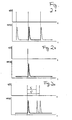
- Fig 2(a) shows heating rate q(t) as a delta function and the corresponding heat flow rate HF(t) for periodic heating rate (part a);
- Fig 2(b) shows a single heating rate pulse;
- Fig. 2(c) shows a single heating rate pulse, which can be followed by another pulse after the time interval t p ' or t p ".
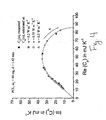
- Fig. 3 shows a polar plot of C app ( ⁇ k ) and C ⁇ ( ⁇ k ) for effective thermal contact K .
- the horizontal and vertical axes show the real and imaginary parts, respectively.
- Fig. 4 shows a polar plot of C ⁇ ( ⁇ k ) , measured and calculated for different values of thermal conductivity ⁇ .
- the horizontal and vertical axes show the real and imaginary parts, respectively.
- Fig. 5 shows a polar plot of C ⁇ ( ⁇ k ) , calculated with optimal parameter ⁇ and measured.
- the horizontal and vertical axes show the real and imaginary parts, respectively.
- Fig. 6 shows a temperature-time program, consisting of 2 K steps in temperature and 30 s isotherms. Temperature steps were programmed as short heating segments with 150 K min-1 heating rate.
- Fig. 7 shows an example of measured heat flow rate HF versus time which corresponds to the temperature-time program, shown in Fig. 4 . The last peak was taken for further data evaluation.
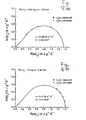
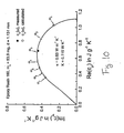
- Fig. 8 shows a polar plot of C ⁇ ( ⁇ k ) , measured and calculated, for PS disks with thickness 1.03 mm (a) and 0.44 mm (b).
- the horizontal and vertical axes show the real and imaginary parts, respectively.
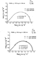
- Fig. 9 shows a polar plot of C ⁇ ( ⁇ k ) , measured and calculated, for PMMA disks with thickness 0.46 mm (a) and 1.052 mm (b).
- the horizontal and vertical axes show the real and imaginary parts, respectively.
- Fig. 10 shows a polar plot of C ⁇ ( ⁇ k ) , measured and calculated, for Epoxy Resin 160 disk with 1.131 mm thickness.
- the horizontal and vertical axes show the real and imaginary parts, respectively.
- Fig. 11 shows a polar plot of C ⁇ ( ⁇ k ) , measured and calculated, for Epoxy Resin 4173.
- the horizontal and vertical axes show the real and imaginary parts, respectively.
- Fig. 12 shows a polar plot of C ⁇ ( ⁇ k ) for a PMMA disk.
- the horizontal and vertical axes show the real and imaginary parts, respectively.
- C ⁇ ( ⁇ k ) values, measured at high frequencies ( ⁇ 7 to ⁇ 10 ), are uncertain.
- Fig. 13 shows a polar plot of C ⁇ ( ⁇ k ) for PS (a) and PMMA (b) disks.
- the horizontal and vertical axes show the real and imaginary parts, respectively. Measured and calculated values do not coincide simultaneously for the whole set of frequencies ⁇ k .
- the present invention resides in control methods for conventional differential analytical apparatus, and is an improvement on the methods currently practiced to control such conventional differential analytical apparatus.
- differential scanning calorimetry in which temperature is the driving variable and heat flow is the characterizing differential physical parameter.
- DSC differential scanning calorimetry
- the present invention could be used with any differential thermal analysis method including Pressure Differential Scanning Calorimetry, Differential Thermal Analysis, Pressure Differential Thermal Analysis, Differential Photocalorimetry, Pressure Differential Photocalorimetry, Differential Thermogravimetry, and Pressure Differential Thermogravimetry, as well as any combination of these techniques.
- the principles and methods described herein with reference to differential scanning calorimetric analysis could be applied to any and all of the thermal analytical methods listed above, as well as to other analytical methods wherein a characterizing differential physical parameter is measured as a function of a driving variable.
- FIG. 1a is a schematic representation of the present invention as it may be used with known Differential Scanning Calorimetry (DSC)(3), for example, Perkin-Elmer Pyris-1 DSC.
- DSC Differential Scanning Calorimetry
- Sample (1) may be any type of sample, however the present invention is appropriate for low thermal conducting solid materials, for examples polymers.
- Low thermal conducting means a material has a thermal conductivity value K in the range of about 0.1 -2 W m-1 K-1.
- Typical polymers include polystyrene, poly(methyl methacrylate), and epoxy resins.
- Grease layer (2) produces an effective amount of thermal contact. In general, utilizing greater amounts of grease (2) in this method produces a better thermal contact. In the preferred embodiment of this invention about 0.5 to about 1 mg of grease (2) is applied to the sample.
- FIG. 1 also shows adiabatic layer (4) located at the upper surface of sample (1).
- the bottom of sample (1) is represented as (5) and is opposite adiabatic layer (4).
- FIG. 1b shows a block diagram of the same conventional differential scanning calorimeter furnace (3).
- FIG. 1a and 1b show schematic representation of a typical sample furnace system where:
- ⁇ and c p are real valued and frequency independent.
- the sample-pan-furnace system may be simplified by excluding the pan.
- the sample disk is measured directly in the DSC furnace. In this case the sample disk is heated only from bottom layer (5), therefore an adiabatic layer (4) is assumed at the upper surface of the sample (1).
- Effective sample thickness d is then the actual sample thickness and the contact area S is the bottom surface area of the disk.
- Fig.1a and 1b show the preferred DSC setup of the present invention where a solid sample is measured directly in the DSC furnace.
- the preferred method is to determine the effective heat capacity C eff ( ⁇ ) at different frequencies, generating a heat capacity spectrum.
- the preferred method of step response analysis in DSC allows the fast generation of heat capacity spectra.
- common temperature modulated calorimetry like 3 ⁇ -method, AC-calorimetry and temperature modulated differential scanning calorimetry (TMDSC)
- periodic perturbations are used to determine dynamic heat capacity.
- this method uses a single step in program temperature followed by an isothermal segment to obtain the spectrum of heat capacity.
- To follow system evolution with time or temperature one can repeat the temperature step several times also in a non-periodic manner (for example, like in StepScan-DSCTM PerkinElmer Instruments). Heating rate and measured heat flow rate are evaluated in time domain. With this method it is possible to cover more than two orders of magnitude in frequency in a single measurement. This allows a dramatic shortening of the measuring time compared to temperature modulated DSC.
- the preferred method of generating frequency dependent quantities by DSC is where the programmed temperature undergoes a sharp single step followed by an isothermal segment. To follow system evolution with time or temperature one can repeat the temperature step several times also in a non-periodic manner. Heating rate and measured heat flow rate are evaluated in time domain by Laplace transformation to obtain the heat capacity spectrum.
- C eff ( ⁇ ) is an effective (apparent) heat capacity of the measured system (which measured by the instrument), which reads:
- a HF ( ⁇ ) is a heat flow rate amplitude
- a T ( ⁇ ) is a temperature amplitude
- a q ( ⁇ ) is a heating rate amplitude.
- the important point is that the heat capacity at frequency ⁇ can be calculated only at a non-zero heating rate amplitude A q ( ⁇ ), which means that the heating rate q(t) should have a periodic component with frequency ⁇ . If the instrument has such a sampling rate, that we get n points per period for HF(t) and q(t) signals, Eq.
- Fig. 2(a) shows a single period of a heating rate function with respect to heat flow rate. If the period between pulses is long enough then the heat flow rate reaches the steady state value before the next temperature step. Since the heat flow rate is periodic, each peak in the heat flow rate starts from the same steady state value. One may set the steady state value of the heat flow rate to zero without influencing the amplitudes of all harmonics. The same can be done with the heating rate.
- the shortest possible basic period t p min of such function is the time the heat flow rate returns back to the steady state value after the perturbation.
- the longest basic period t p max is the time interval the heat flow rate has been actually measured after the temperature step. Since one may vary the basic period in a certain range for this single step in temperature one may generate a continuous spectrum of heating rate instead of a discreet spectrum in case of the periodic q(t). Then C eff ( ⁇ ) can be calculated for a continuous frequency range ⁇ ⁇ 2 ⁇ / t p max .
- heat flow rate does not contribute to the Fourier integral any more after its relaxation back to the steady state value.
- the only variable for C eff ( ⁇ ) determination is the frequency ⁇ .
- the area under the heat flow rate peak in time domain is the total amount of heat absorbed by the sample due to the stepwise increase of temperature.
- the single step measurement can be analyzed as a fictitious periodic measurement under condition that q(t) and HF(t) start and end at the same steady state values. Therefore to get correct G eff ( ⁇ ) values by Eq. (1) the measurements should start from steady state.
- the step in temperature can be approximated as a very steep heating (or cooling) ramp in short time. For example we have used a programmed heating rate of 75 K/min for 0.8 second and 1.6 second to have 1 K and 2 K temperature steps, respectively. After the temperature step the heat flow rate HF(t) should be recorded until it returns back to steady state.
- the measured step in the temperature-time profile is not as sharp as it was programmed because of instrumental delay.
- the power compensated system having much smaller furnaces than the heat flux system, responds much faster and follows more tightly the program temperature.
- C eff ( ⁇ ) determination by Eq. (1) a large part of the instrumental delay can be eliminated by using the measured heating rate instead of programmed one.
- C eff ( ⁇ ) values correspond to some average values of actual C eff ( ⁇ ) spectrum in the temperature range (T 0 , T 0 + ⁇ T) and in the time interval (t 0 , t 0 + t p max ), where T 0 is the starting temperature of the step measurement, ⁇ T is the height of the temperature step, t 0 is the starting time, t p max is the total measuring time of the single step.
- T 0 is the starting temperature of the step measurement
- ⁇ T is the height of the temperature step
- t 0 is the starting time
- t p max is the total measuring time of the single step.
- One may monitor the evolution of the C eff ( ⁇ ) spectrum with changing temperature or with time (e.g. during isothermal crystallization), one can repeat the step perturbation at another temperature or at another time.
- the effective heat capacity C eff ( ⁇ ) at different frequencies is preferably calculated from step response analysis as a ratio of heat flow rate amplitude A HF and heating rate amplitude A q :
- C eff ⁇ A HF
- points of heat flow rate, HF i , and heating rate, q i are preferably taken both with the same sampling rate (number of points per unit time).
- the points are collected from the beginning of the temperature step until the heat flow reaches the steady state value at the isotherm, having in total n points.
- the first parameter of the system the specific heat capacity c p
- c p C eff 0 m s
- C app ⁇ C ⁇ ⁇ 1 - i ⁇ K ⁇ C ⁇ ⁇
- C ⁇ ( ⁇ ) is the apparent heat capacity in a case of ideal thermal contact between the sample and the furnace. It is the apparent heat capacity which is measured directly on the bottom surface of the sample.
- K is K because C app ( ⁇ ) is measured by DSC.
- the second parameter of the system is determined by describing C ⁇ ( ⁇ ) on a solid curve.
- the correct value for K is then the value at which all C ⁇ ( ⁇ k ) points, calculated by Eq.(5), lie on the theoretical curve.
- Fig. 3 shows values of C app ( ⁇ k ) for a set of different frequencies ⁇ k and C ⁇ ( ⁇ k ) for three different values of K at 0.04 W K -1 , 0.029 W K -1 , and 0.02 W K -1 .
- the horizontal and vertical axes show the real and imaginary parts, respectively.
- Fig. 4 shows a polar plot of C ⁇ ( ⁇ k ) , measured and calculated for different values of thermal conductivity ⁇ .
- the horizontal and vertical axes show the real and imaginary parts, respectively.
- Fig. 6 shows a temperature-time program, consisting of 2 K steps in temperature and 30 s isotherms. Temperature steps were programmed as short heating segments with 150 K min-1 heating rate. Temperature-time program shown in Fig. 6 was used to generate the spectrum of apparent heat capacities in the examples below.
- Fig. 7 shows an example of measured heat flow rate HF versus time which corresponds to the temperature-time program, shown in Fig. 6 . The last peak was taken for further data evaluation. Initial isotherm of 1 min was added to check whether heat flow drift at steady state is remarkable. Fig. 7 shows corresponding heat flow rate after empty furnace correction is shown (Since we did not use a pan we subtracted the heat flow measured with an empty furnace.)
- Fig. 8 shows a polar plot of C ⁇ ( ⁇ k ) , measured and calculated, for PS disks with thickness 1.03 mm (a) and 0.44 mm (b).
- the horizontal and vertical axes show the real and imaginary parts, respectively.
- Two PS disks with different thickness give quite different values of C ⁇ ( ⁇ k ) at the same set of frequencies.
- both sets of C ⁇ ( ⁇ k ) give almost the same value of thermal conductivity ⁇ of about 0.17 W m -1 K -1 that is the property of the material.
- Fig. 9 shows a polar plot of C ⁇ ( ⁇ k ), measured and calculated, for PMMA disks with thickness 0.46 mm (a) and 1.052 mm (b).
- the horizontal and vertical axes show the real and imaginary parts, respectively.
- Two PMMA disks with different thickness give quite different values of C ⁇ ( ⁇ k ) at the same set of frequencies. However both sets of C ⁇ ( ⁇ k ) give almost the same value of thermal conductivity ⁇ of about 0.214 W m -1 K -1 that is the property of the material.
- ⁇ 0.215 W m -1 K -1
- specific heat capacity in these two measurements is different.
- Additional heat capacity of the grease in second measurement increases total measured heat capacity which is normalized to the same sample mass.
- the measured points coincide with calculated ones only to some extend. There is always some scatter in the data.
- Fig. 10 shows a polar plot of C ⁇ ( ⁇ k ), measured and calculated, for Epoxy Resin 160 disk with 1.131 mm thickness.
- the horizontal and vertical axes show the real and imaginary parts, respectively.
- Fig. 11 shows a polar plot of C ⁇ ( ⁇ k ), measured and calculated, for Epoxy Resin 4173.
- the horizontal and vertical axes show the real and imaginary parts, respectively.
- the same measured data set can give slightly lower thermal contact K and higher thermal conductivity ⁇ or higher K and lower ⁇ - measured and calculated points in both cases more or less coincide. It is impossible to narrow the range of K and into get the correct pair.
- Fig. 12 shows a polar plot of C ⁇ ( ⁇ k ) for a PMMA disk.
- the horizontal and vertical axes show the real and imaginary parts, respectively.
- C ⁇ ( ⁇ k ) values, measured at high frequencies ( ⁇ 7 to ⁇ 10 ), are uncertain.
- Fig. 13 shows a polar plot of C ⁇ ( ⁇ k ) for PS (a) and PMMA (b) disks.
- the horizontal and vertical.axes show the real and imaginary parts, respectively. Measured and calculated values do not coincide simultaneously for the whole set of frequencies ⁇ k .
- the one dimensional model used for calculation could not give exact values of thermal conductivity. But one can get some range of possible value of thermal conductivity. From the width of the range one gets an impression about the validity of the model to describe the given experimental conditions, or, put another way, how faulty were the experimental conditions.
- PMMA samples with know thermal conductivity were measured (ASTM interlabarotory test for thermal conductivity by modulated temperature DSC). The measurements were performed by Perkin-Elmer Pyris-1 DSC and Lauda RC6 cooling system. The sample was prepared and thermal conductivity was determined the same way as in example 1. Temperature-time program shown in Fig. 8 was used to generate the spectrum of apparent heat capacity. Corresponding heat flow rate after empty furnace correction is shown at Fig. 9 (since a pan was not utilized, it is necessary to subtract the heat flow measured with an empty furnace). The results of thermal conductivity determination are shown in Table 1 below. Fig. 11 show two PMMA discs with different thickness give different values of C ⁇ ( ⁇ k ) at the same set of frequencies. Both sets of C ⁇ ( ⁇ k ) give almost the same value of thermal conductivity ⁇ of about 0.214 W m -1 K -1 that is the property of the material.
- Epoxy resin 4173 (provided by Mathis Instruments) with know thermal conductivity was measured. The measurements were performed by Perkin-Elmer Pyris-1 DSC and Lauda RC6 cooling system. The sample was prepared and thermal conductivity was determined the same way as in example 3. Temperature-time program shown in Fig. 8 was used to generate the spectrum of apparent heat capacity. Corresponding heat flow rate after empty furnace correction is shown at Fig. 9 (since a pan was not utilized, it is necessary to subtract the heat flow measured with an empty furnace). The results of thermal conductivity determination are shown in Table 1 below.
- Table 1 Comparative thermal conductivities measured at 51 °C for four different samples material measured ⁇ in W m -1 K -1 expected ⁇ in W m -1 K -1 PS 0.168-0.172 0.1562 (when taken at 47°C) PMMA 0.212-0.215 0.197 (when taken at 47.2°C) epoxy resin 160 0.63 0.61 epoxy resin 4173 1.70-1.85 1.83
Landscapes
- Chemical & Material Sciences (AREA)
- General Health & Medical Sciences (AREA)
- Life Sciences & Earth Sciences (AREA)
- Health & Medical Sciences (AREA)
- Analytical Chemistry (AREA)
- Biochemistry (AREA)
- Physics & Mathematics (AREA)
- General Physics & Mathematics (AREA)
- Immunology (AREA)
- Pathology (AREA)
- Engineering & Computer Science (AREA)
- Chemical Kinetics & Catalysis (AREA)
- Combustion & Propulsion (AREA)
- Investigating Or Analyzing Materials Using Thermal Means (AREA)
Claims (22)
- Ein Verfahren zum Messen der thermischen Leitfähigkeit einer Probe, das Verfahren mit dem Schritt:(a) Vorbereiten einer Probe des Materials in der Form eines dünnen Wafers mit einer bekannten Dicke, bekannten Abmessungen und einer bekannten Dichte;
wobei das Verfahren durch die folgenden Schritte gekennzeichnet ist:(b) Messen der effektiven Wärmekapazität der Probe und Erzeugen eines Spektrums der effektiven Wärmekapazität;(c) Bestimmen der scheinbaren Wärmekapazität, indem der Wert des Spektrums der effektiven Wärmekapazität aus Schritt (b) angepasst wird;(d) Bestimmen der spezifischen Wärmekapazität der Probe;(e) Bestimmen des effektiven thermischen Kontakts der Probe;(f) Berechnen der thermischen Leitfähigkeit des Materials basierend zumindest auf der scheinbaren Wärmekapazität der Probe, des effektiven thermischen Kontakts der Probe und der spezifischen Wärmekapazität der Probe. - Das Verfahren nach Anspruch 1, dadurch gekennzeichnet, dass die Dicke der Probe ungefähr einen Millimeter oder weniger beträgt.
- Das Verfahren nach Anspruch 1, gekennzeichnet durch einen weiteren Schritt eines Aufbringens einer Masse zum Wärmeableiten an der Probe.
- Das Verfahren nach Anspruch 3, dadurch gekennzeichnet, dass es sich bei der Masse zum Wärmeableiten um Fett handelt.
- Das Verfahren nach Anspruch 1, dadurch gekennzeichnet, dass der Wafer die Form einer kreisförmigen Scheibe hat.
- Das Verfahren nach Anspruch 1, dadurch gekennzeichnet, dass die Probe ein Polymer ist.
- Das Verfahren nach Anspruch 6, dadurch gekennzeichnet, dass das Polymer ein Material mit einer geringen thermischen Leitfähigkeit aufweist, wobei der Wert der thermischen Leitfähigkeit in einem Bereich von ungefähr 0,1 bis ungefähr 2 W m-1 K-1 liegt.
- Das Verfahren nach Anspruch 6, dadurch gekennzeichnet, dass das Polymer aus einer Gruppe ausgewählt ist, die Gruppe bestehend aus Polystyren, PMMA, Epoxydharz 160, Epoxydharz 4173 und Kombinationen aus diesen Stoffen.
- Das Verfahren nach Anspruch 1, gekennzeichnet durch den weiteren Schritt eines Platzierens der Probe in einer Probeaufnahme eines Kalorimeters, das mit differentieller Erfassung arbeitet.
- Das Verfahren nach Anspruch 9, dadurch gekennzeichnet, dass der Schritt des Messens der effektiven Wärmekapazität der Probe unter Verwendung des Kalorimeters, das mit differentieller Erfassung arbeitet, des Weiteren einen Schritt eines Berechnens eines Verhältnisses der Amplitude der Wärmeflussrate und der Amplitude der Heizrate aufweist.
- Das Verfahren nach Anspruch 10, dadurch gekennzeichnet, dass es ferner eine Verwendung einer Laplace-Transformation aufweist, um ein Spektrum der Wärmekapazität zu erzeugen.
- Das Verfahren nach Anspruch 10, dadurch gekennzeichnet, dass es ferner eine Verwendung einer Fourier-Transformation aufweist, um ein Spektrum der Wärmekapazität zu erzeugen.
- Das Verfahren nach Anspruch 10, dadurch gekennzeichnet, dass die Formel

- Das Verfahren nach Anspruch 10, dadurch gekennzeichnet, dass die Temperatur zumindest einem Temperaturschritt unterworfen wird, dem zumindest ein isothermer Abschnitt folgt, um ein Spektrum der Wärmekapazität zu erzeugen.
- Das Verfahren nach Anspruch 1, dadurch gekennzeichnet, dass der Schritt des Bestimmens der scheinbaren Wärmekapazität ein Korrigieren im Hinblick auf eine Verzögerung der Instrumente aufweist.
- Das Verfahren nach Anspruch 15, dadurch gekennzeichnet, dass der Schritt des Bestimmens der scheinbaren Wärmekapazität des Weiteren die Anwendung der Formel

- Das Verfahren nach Anspruch 1, dadurch gekennzeichnet, dass der Schritt des Bestimmens der spezifischen Wärmekapazität der Probe die Anwendung der Formel

- Das Verfahren nach Anspruch 1, dadurch gekennzeichnet, dass der Schritt des Bestimmens des effektiven thermischen Kontakts der Probe ein Beschreiben von Cα(ω) auf einer durchgehenden Kurve aufweist, wobei es sich bei der durchgehenden Kurve um eine Repräsentation in Polarkoordinaten handelt, die nur von dem Wert Cα(ω = 0) abhängig ist, und wobei der effektive thermische Kontakt der Probe dann der Wert ist, bei dem alle Punkte Cα(ωk) auf der theoretischen Kurve liegen.
- Das Verfahren nach Anspruch 1, dadurch gekennzeichnet, dass der Schritt des Berechnens der thermischen Leitfähigkeit des Materials das Anwenden der Formel

- Das Verfahren nach Anspruch 1, dadurch gekennzeichnet, dass der Schritt des Berechnens der thermischen Leitfähigkeit einer Probe mittels eines Computers bestimmt wird.
- Das Verfahren nach Anspruch 1, dadurch gekennzeichnet, dass der Schritt des Berechnens der thermischen Leitfähigkeit einer Probe durch eine Tabelle in MS-Excel™ mit Makros in Visual Basic™ realisiert wird.
- Das Verfahren nach Anspruch 1, dadurch gekennzeichnet, dass der Schritt des Messens der effektiven Wärmekapazität der Probe ein Messen der Wärmekapazität der Probe mit zumindest zwei verschiedenen Modulationsfrequenzen aufweist und wobei nur eine Messung für die effektive Wärmekapazität der Probe bestimmt wurde.
Applications Claiming Priority (3)
| Application Number | Priority Date | Filing Date | Title |
|---|---|---|---|
| US09/877,390 US6497509B2 (en) | 2000-06-08 | 2001-06-08 | Method for measuring absolute value of thermal conductivity |
| US877390 | 2001-06-08 | ||
| PCT/US2001/018769 WO2002101371A1 (en) | 2001-06-08 | 2001-06-09 | Method for measuring absolute value of thermal conductivity |
Publications (3)
| Publication Number | Publication Date |
|---|---|
| EP1402249A1 EP1402249A1 (de) | 2004-03-31 |
| EP1402249A4 EP1402249A4 (de) | 2006-12-27 |
| EP1402249B1 true EP1402249B1 (de) | 2010-05-05 |
Family
ID=25369883
Family Applications (1)
| Application Number | Title | Priority Date | Filing Date |
|---|---|---|---|
| EP01944424A Expired - Lifetime EP1402249B1 (de) | 2001-06-08 | 2001-06-09 | Verfahren zur messung des absolutwerts der wärmeleitfähigkeit |
Country Status (3)
| Country | Link |
|---|---|
| EP (1) | EP1402249B1 (de) |
| DE (1) | DE60142083D1 (de) |
| WO (1) | WO2002101371A1 (de) |
Families Citing this family (1)
| Publication number | Priority date | Publication date | Assignee | Title |
|---|---|---|---|---|
| RU2263901C1 (ru) * | 2004-05-25 | 2005-11-10 | Тамбовский государственный технический университет (ТГТУ) | Способ неразрушающего контроля комплекса теплофизических характеристик твердых строительных материалов |
Family Cites Families (13)
| Publication number | Priority date | Publication date | Assignee | Title |
|---|---|---|---|---|
| US4255961A (en) * | 1978-10-17 | 1981-03-17 | University Of Va. Alumni Patents Foundation | Differential calorimeter based on the heat leak principle |
| PL158642B1 (pl) * | 1988-05-20 | 1992-09-30 | Polska Akad Nauk Centrum | Sposób i urzadzenie do wyznaczania wspólczynnika przewodnictwa cieplnego materialówUprawniony z patentu:Polska Akadem ia N auk C entrum B adanM olekularnych i M akrom olekularnych, PL |
| US5099441A (en) * | 1988-05-31 | 1992-03-24 | Eastman Kodak Company | Method for determining thermal conductivity incorporating differential scanning calorimetry |
| US5224775C2 (en) * | 1992-03-02 | 2002-04-23 | Ta Instr Inc | Method and apparatus for modulated differential analysis |
| US5335993A (en) * | 1992-03-02 | 1994-08-09 | Ta Instruments, Inc. | Method and apparatus for thermal conductivity measurements |
| US5439291C1 (en) * | 1992-03-02 | 2002-04-16 | Ta Instr Inc | Method and apparatus for ac differential thermal analysis |
| US5711604A (en) * | 1993-12-14 | 1998-01-27 | Seiko Instruments Inc. | Method for measuring the coefficient of heat conductivity of a sample |
| US5549387A (en) * | 1994-06-01 | 1996-08-27 | The Perkin-Elmer Corporation | Apparatus and method for differential analysis using real and imaginary signal components |
| CA2126481C (en) * | 1994-06-22 | 2001-03-27 | Andreas Mandelis | Non-contact photothermal method for measuring thermal diffusivity and electronic defect properties of solids |
| US5688049A (en) * | 1996-01-25 | 1997-11-18 | Inrad | Method and apparatus for measuring the thermal conductivity of thin films |
| EP0883801B1 (de) * | 1996-11-01 | 2004-09-15 | TA Instruments, Inc. | Differentialabtastkalorimeter |
| US6200022B1 (en) * | 1997-04-21 | 2001-03-13 | Ta Instruments, Inc. | Method and apparatus for localized dynamic mechano-thermal analysis with scanning probe microscopy |
| US6142662A (en) * | 1998-06-16 | 2000-11-07 | New Jersey Institute Of Technology | Apparatus and method for simultaneously determining thermal conductivity and thermal contact resistance |
-
2001
- 2001-06-09 EP EP01944424A patent/EP1402249B1/de not_active Expired - Lifetime
- 2001-06-09 DE DE60142083T patent/DE60142083D1/de not_active Expired - Lifetime
- 2001-06-09 WO PCT/US2001/018769 patent/WO2002101371A1/en not_active Ceased
Also Published As
| Publication number | Publication date |
|---|---|
| EP1402249A4 (de) | 2006-12-27 |
| EP1402249A1 (de) | 2004-03-31 |
| DE60142083D1 (de) | 2010-06-17 |
| WO2002101371A1 (en) | 2002-12-19 |
Similar Documents
| Publication | Publication Date | Title |
|---|---|---|
| US6497509B2 (en) | Method for measuring absolute value of thermal conductivity | |
| US5711604A (en) | Method for measuring the coefficient of heat conductivity of a sample | |
| Wunderlich et al. | Temperature-modulated differential scanning calorimetry of reversible and irreversible first-order transitions | |
| US6561692B2 (en) | Differential scanning calorimeter | |
| US5599104A (en) | Thermal analysis instrument | |
| EP0634649B1 (de) | Verfahren und Vorrichtung zur Messung der Wärmeleitfähigkeit | |
| Merzlyakov et al. | Thermal conductivity from dynamic response of DSC | |
| Huth et al. | Differential AC-chip calorimeter for glass transition measurements in ultra thin polymeric films | |
| US6170984B1 (en) | Apparatus and method for differential analysis using real and imaginary signal components | |
| Ahrenberg et al. | In situ investigation of vapor-deposited glasses of toluene and ethylbenzene via alternating current chip-nanocalorimetry | |
| McHugh et al. | Determination and review of specific heat capacity measurements during isothermal cure of an epoxy using TM-DSC and standard DSC techniques | |
| US6488406B2 (en) | Differential scanning calorimeter | |
| US5713665A (en) | Method and apparatus for thermal diffusivity measurement | |
| US20110013663A1 (en) | Thermal analysis method and apparatus | |
| US6551835B1 (en) | Method and apparatus for thermally analyzing a material | |
| Lacey et al. | Theory and practice of modulated temperature differential scanning calorimetry | |
| Weyer et al. | Application of an extended Tool–Narayanaswamy–Moynihan model. Part 2. Frequency and cooling rate dependence of glass transition from temperature modulated DSC | |
| US7626144B2 (en) | Method and apparatus for rapid temperature changes | |
| JP3556227B2 (ja) | 実部信号成分と虚部信号成分を用いた示差分析のための装置および方法 | |
| JP3103963B2 (ja) | 熱伝導率の測定方法 | |
| CN113640343A (zh) | 基于激光功率激励的差式扫描量热仪温度标定与重构方法 | |
| EP1402249A1 (de) | Verfahren zur messung des absolutwerts der wärmeleitfähigkeit | |
| Xu et al. | Study of temperature profile and specific heat capacity in temperature modulated DSC with a low sample heat diffusivity | |
| Pak et al. | Heat capacity by sawtooth-modulated, standard heat-flux differential scanning calorimeter with close control of the heater temperature | |
| Höhne et al. | DSC curves and further evaluations |
Legal Events
| Date | Code | Title | Description |
|---|---|---|---|
| PUAI | Public reference made under article 153(3) epc to a published international application that has entered the european phase |
Free format text: ORIGINAL CODE: 0009012 |
|
| 17P | Request for examination filed |
Effective date: 20020308 |
|
| AK | Designated contracting states |
Kind code of ref document: A1 Designated state(s): AT BE CH CY DE DK ES FI FR GB GR IE IT LI LU MC NL PT SE TR |
|
| A4 | Supplementary search report drawn up and despatched |
Effective date: 20061124 |
|
| RIC1 | Information provided on ipc code assigned before grant |
Ipc: G01N 25/18 20060101AFI20030106BHEP Ipc: G01N 25/48 20060101ALI20061120BHEP Ipc: G01N 25/00 20060101ALI20061120BHEP |
|
| 17Q | First examination report despatched |
Effective date: 20071121 |
|
| GRAP | Despatch of communication of intention to grant a patent |
Free format text: ORIGINAL CODE: EPIDOSNIGR1 |
|
| GRAS | Grant fee paid |
Free format text: ORIGINAL CODE: EPIDOSNIGR3 |
|
| RAP1 | Party data changed (applicant data changed or rights of an application transferred) |
Owner name: PERKINELMER HEALTH SCIENCES, INC. |
|
| GRAA | (expected) grant |
Free format text: ORIGINAL CODE: 0009210 |
|
| AK | Designated contracting states |
Kind code of ref document: B1 Designated state(s): DE FR GB IT |
|
| REG | Reference to a national code |
Ref country code: GB Ref legal event code: FG4D |
|
| REF | Corresponds to: |
Ref document number: 60142083 Country of ref document: DE Date of ref document: 20100617 Kind code of ref document: P |
|
| PLBE | No opposition filed within time limit |
Free format text: ORIGINAL CODE: 0009261 |
|
| STAA | Information on the status of an ep patent application or granted ep patent |
Free format text: STATUS: NO OPPOSITION FILED WITHIN TIME LIMIT |
|
| PG25 | Lapsed in a contracting state [announced via postgrant information from national office to epo] |
Ref country code: IT Free format text: LAPSE BECAUSE OF FAILURE TO SUBMIT A TRANSLATION OF THE DESCRIPTION OR TO PAY THE FEE WITHIN THE PRESCRIBED TIME-LIMIT Effective date: 20100505 |
|
| 26N | No opposition filed |
Effective date: 20110208 |
|
| REG | Reference to a national code |
Ref country code: DE Ref legal event code: R097 Ref document number: 60142083 Country of ref document: DE Effective date: 20110207 |
|
| REG | Reference to a national code |
Ref country code: FR Ref legal event code: PLFP Year of fee payment: 16 |
|
| REG | Reference to a national code |
Ref country code: FR Ref legal event code: PLFP Year of fee payment: 17 |
|
| REG | Reference to a national code |
Ref country code: FR Ref legal event code: PLFP Year of fee payment: 18 |
|
| PGFP | Annual fee paid to national office [announced via postgrant information from national office to epo] |
Ref country code: FR Payment date: 20200526 Year of fee payment: 20 Ref country code: DE Payment date: 20200527 Year of fee payment: 20 |
|
| PGFP | Annual fee paid to national office [announced via postgrant information from national office to epo] |
Ref country code: GB Payment date: 20200527 Year of fee payment: 20 |
|
| REG | Reference to a national code |
Ref country code: DE Ref legal event code: R071 Ref document number: 60142083 Country of ref document: DE |
|
| REG | Reference to a national code |
Ref country code: GB Ref legal event code: PE20 Expiry date: 20210608 |
|
| PG25 | Lapsed in a contracting state [announced via postgrant information from national office to epo] |
Ref country code: GB Free format text: LAPSE BECAUSE OF EXPIRATION OF PROTECTION Effective date: 20210608 |