EP1441238A2 - Modellierung von einem in-situ Ölreservoir unter berücksichtigung eingeschränkter Abgeleiteten - Google Patents
Modellierung von einem in-situ Ölreservoir unter berücksichtigung eingeschränkter Abgeleiteten Download PDFInfo
- Publication number
- EP1441238A2 EP1441238A2 EP04001565A EP04001565A EP1441238A2 EP 1441238 A2 EP1441238 A2 EP 1441238A2 EP 04001565 A EP04001565 A EP 04001565A EP 04001565 A EP04001565 A EP 04001565A EP 1441238 A2 EP1441238 A2 EP 1441238A2
- Authority
- EP
- European Patent Office
- Prior art keywords
- model
- reservoir
- input
- function
- constraints
- Prior art date
- Legal status (The legal status is an assumption and is not a legal conclusion. Google has not performed a legal analysis and makes no representation as to the accuracy of the status listed.)
- Granted
Links
Images




Classifications
-
- E—FIXED CONSTRUCTIONS
- E21—EARTH OR ROCK DRILLING; MINING
- E21B—EARTH OR ROCK DRILLING; OBTAINING OIL, GAS, WATER, SOLUBLE OR MELTABLE MATERIALS OR A SLURRY OF MINERALS FROM WELLS
- E21B49/00—Testing the nature of borehole walls; Formation testing; Methods or apparatus for obtaining samples of soil or well fluids, specially adapted to earth drilling or wells
Definitions
- the present invention generally relates to the fields of predictive modeling and hydrocarbon, e.g., oil and/or natural gas, production, and more particularly to parameterization of steady-state empirical models of in-situ hydrocarbon reservoirs with derivative constraints.
- predictive modeling and hydrocarbon e.g., oil and/or natural gas
- Predictive models generally refer to any representation of a system or process which receives input data or parameters related to system or model attributes and/or external circumstances/environment and generates output indicating the behavior of the system or process under those parameters.
- the model or models may be used to predict behavior or trends based upon previously acquired data.
- predictive models including linear, non-linear, analytic, and empirical models, among others, several types of which are described in more detail below.
- Optimization generally refers to a process whereby past (or synthesized) data related to a system or process are analyzed or used to select or determine optimal parameter sets for operation of the system or process.
- the predictive models mentioned above may be used in an optimization process to test or characterize the behavior of the system or process under a wide variety of parameter values. The results of each test may be compared, and the parameter set or sets corresponding to the most beneficial outcomes or results may be selected for implementation in the actual system or process.
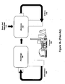
- Figure 1A illustrates a general optimization process as applied to an industrial process 104, such as a manufacturing plant, according to the prior art. It may be noted that the optimization techniques described with respect to the manufacturing plant are generally applicable to all manner of systems and processes.
- the operation of the process 104 generates information or data 106 which is typically analyzed and/or transformed into useful knowledge 108 regarding the system or process.
- the information 106 produced by the process 104 may comprise raw production numbers for the plant which are used to generate knowledge 108, such as profit, revenue flow, inventory depth, etc.
- This knowledge 108 may then be analyzed in the light of various goals and objectives 112 and used to generate decisions 110 related to the operation of the system or process 104 subject to various goals and objectives 112 specified by the analyst.
- an "objective" may include a goal or desired outcome of an optimization process.
- Example goals and objectives 112 may include profitability, schedules, inventory levels, cash flow, revenue growth, risk, or any other attribute which the user may wish to minimize or maximize.
- These goals and objectives 112 may be used to select from among the possible decisions 110, where the decisions may comprise various parameter values over which the user may exercise control.
- the selected decision(s) may then determine one or more actions 114 to be applied to the operation of the system or process 104.
- the subsequent operation of the system or process 104 then generates more information 106, from which further knowledge 108 may be generated, and so on in an iterative fashion. In this way, the operation of the process 104 may be "tuned" to perform in a manner which most closely meets the goals and objectives of the business or enterprise.
- Figure 1B illustrates an optimization system where a computer based optimization system 102 operates in conjunction with a process 104 to optimize the process, according to the prior art.
- the computer system 102 executes software programs (including computer based predictive models) which receive process data 106 from the process 104 and generate optimized decisions and/or actions which may then be applied to the process 104 to improve operations based on the goals and objectives.
- predictive systems may be characterized by the use of an internal model which represents a process or system 104 for which predictions are made.
- predictive model types may be linear, non-linear, stochastic, or analytical, among others.
- non-linear models may generally be preferred due to their ability to capture non-linear dependencies among various attributes of the phenomena.
- Examples of non-linear models may include neural networks and support vector machines (SVMs).
- the types of models used in optimization systems include fundamental or analytic models which use known information about the process 104 to predict desired unknown information, such as product conditions and product properties.
- a fundamental model may be based on scientific and engineering principles. Such principles may include the conservation of material and energy, the equality of forces, and so on. These basic scientific and engineering principles may be expressed as equations which are solved mathematically or numerically, usually using a computer program. Once solved, these equations may give the desired prediction of unknown information.
- Empirical models also referred to as computer-based statistical models, may also be used to model the system or process 104 in an optimization system. Such models typically use known information about process to determine desired information that may not be easily or effectively measured.
- a statistical empirical model may be based on the correlation of measurable process conditions or product properties of the process. Examples of computer-based empirical or statistical models include neural networks and support vector machines.
- model builder would need to have a base of experience, including known information and actual measurements of desired unknown information.
- known information may include the temperature at which the plastic is processed.
- Actual measurements of desired unknown information may be the actual measurements of the color of the plastic.
- a mathematical relationship (i.e., an equation) between the known information and the desired unknown information may be created by the developer of the empirical statistical model.
- the relationship may contain one or more parameters or constants (which may be assigned numerical values) which affect the value of the predicted information from any given known information. In an analytic model these parameters are referred to as coefficients.
- a computer program may use many different measurements of known information, with their corresponding actual measurements of desired unknown information, to adjust these constants so that the best possible prediction results may be achieved by the empirical statistical model.
- Such a computer program may use non-linear regression or any of various other techniques to determine the values of the parameters.
- Computer-based statistical models may sometimes predict product properties which may not be well described by computer fundamental models.
- computer statistical models may include the following:
- Predictive model types also include procedural or recipe based models. These models typically comprise a number of steps whose performance emulates or models the phenomenon or process. Thus, procedural or recipe models are not based on understanding of the fundamental processes of a system, but instead, are generally constructed with an empirical or emulative approach.
- a model is parameterized or trained with training data, e.g., historical or synthesized data, in order to reflect salient attributes and behaviors of the phenomena being modeled.
- training data e.g., historical or synthesized data
- sets of training data may be provided as inputs to the model, and the model output may be compared to corresponding sets of desired outputs.
- the resulting error is often used to adjust weights or coefficients in the model until the model generates the correct output (within some error margin) for each set of training data.
- the model is considered to be in "training mode" during this process.
- the model may receive real-world data as inputs, and provide predictive output information which may be used to control or make decisions regarding the modeled phenomena.
- a predictive model historical data are gathered, e.g., information generated by the system or process 104 in previous operations.
- the historical data are typically preprocessed to put the data into a form useful for creating, parameterizing, and/or training a predictive model.
- the predictive model is then created, parameterized, and/or trained.
- the predictive model could be any of a variety of model types, depending upon the particular application and/or available resources.
- the model may then be analyzed. In other words, various tools may be applied to discover the behavior of the model.
- the model may be modified or tuned to more accurately represent the phenomenon, system, or process being modeled. Further historical data may then be used to further parameterize or train the model, and the model analyzed and modified to further refine the model behavior. This process may be performed iteratively until the model is parameterized or trained appropriately.
- the model may be deployed.
- the model may be included in an optimization system 100 which is coupled to a real world process or system 104, as described above with reference to Figures 1A and 1B.
- predictive models may be used by a decision-maker associated with an operation or enterprise to select an optimal course of action or optimal course of decision.
- the optimal course of action or decision may include a sequence or combination or actions and/or decisions.
- optimization may be used to select an optimal course of action for production of hydrocarbons, e.g., petroleum or oil, natural gas, etc., from a reservoir, such as determining when and where to drill wells, what pressures to maintain, and so forth.
- decision variables are those variables that the decision-maker may change to affect the outcome of the optimization process 100.
- pressure and injection flows may be decision variables.
- exital variables are those variables that are not under the control of the decision-maker. In other words, the external variables are not changed in the decision process but rather are taken as givens.
- external variables may include variables such as hydrocarbon production or output.
- Figure 2 is a block diagram of a predictive model 215 as used in an optimization system 100, according to the prior art.
- the model 215 may receive input in the form of external variables 212 and decision variables 214, defined above, and generate action variable 218.
- action variables are those variables that propose or suggest a set of actions for an input set of decision and external variables.
- the action variables may comprise predictive metrics for a behavior.
- the action variables may include the productivity of an oil or gas well or group of wells.
- predictive models may be used for analysis, control, and decision making in many areas, including hydrocarbon production, manufacturing, process control, plant management, quality control, optimized decision making, e-commerce, financial markets and systems, or any other field where predictive modeling may be useful.
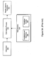
- Figures 3A and 3B illustrate a general optimization system and process using predictive models with an optimizer to generate optimal decision variables, according to the prior art.
- FIG. 3A is a block diagram which illustrates an overview of optimization according to the prior art.
- an optimization process 100 may accept the following elements as input: information 302, such as oil well or reservoir conditions, predictive model(s) such as hydrocarbon reservoir or well model(s) 304, and one or more constraints and/or objectives 306, such as injection rates, mass balances, and desired production rates or profitability.
- information 302 such as oil well or reservoir conditions
- predictive model(s) such as hydrocarbon reservoir or well model(s) 304
- constraints and/or objectives 306 such as injection rates, mass balances, and desired production rates or profitability.
- constraints and/or objectives 306 such as injection rates, mass balances, and desired production rates or profitability.
- constraints and/or objectives 306 such as injection rates, mass balances, and desired production rates or profitability.
- constraints and/or objectives 306 such as injection rates, mass balances, and desired production rates or profitability.
- constraints and/or objectives 306 such as injection rates, mass balances, and desired production rates or profitability.
- each of the predictive model(s) 304 may be an oil or gas well model, and may correspond to a different well 302.
- Figure 3B illustrates data flow in the optimization system of Figure 3A.
- the information 202 typically includes decision variables 214 and external variables 212, as described above.
- the information 302, including decision variables 214 and external variables 212, is input into the predictive model(s) 304 to generate the action variables 218.
- each of the predictive model(s) 304 may correspond to one of the oil or reservoir conditions 302, where each of the conditions 302 includes appropriate decision variables 214 and external variables 212.
- the predictive model(s) 304 may include well or reservoir model(s) as well as other models.
- the predictive model(s) 304 can generally take any of several forms, as described above, including trained neural nets, statistical models, analytic models, and any other suitable models for generating predictive metrics, and may take various forms including linear or non-linear, or may be derived from empirical data or from managerial judgment.
- the action variables 218 generated by the model(s) 304 are used to formulate constraint(s) and the objective function 306 via formulas.
- a data calculator 320 generates the constraint(s) and objective 306 using the action variables 218 and potentially other data and variables.
- the formulations of the constraint(s) and objective 306 may include financial formulas such as formulas for determining net operating income over a certain time period.
- the constraint(s) and objective 306 may be input into an optimizer 324, which may comprise, for example, a custom-designed process or a commercially available "off the shelf" product.
- the optimizer may then generate the optimal decision variables 312 which have values optimized for the goal specified by the objective function and subject to the constraint(s) 306.
- a typical reservoir engineering problem is to determine the injection rates that maximize field production.
- a rigorous simulation model is typically fit to field data in what is known as a "history match".
- a man-year or more may be spent parameterizing or tuning the model so that it replicates what the oil field has done historically. After a large fraction of the project budget is used up, e.g., 85%, the reservoir engineers typically make 15 or 20 runs of the simulation and then make their best guess for the injection rates.
- the present invention comprises various embodiments of a system and method for parameterizing steady-state models using derivative constraints. More specifically, embodiments of a system and method are described for parameterization of a compact empirical model of an in-situ hydrocarbon reservoir using derivative constraints and an optimizer.
- the model may represent an in-situ hydrocarbon reservoir and/or operations related to hydrocarbon production from the reservoir, although the methods described herein are broadly applicable in other fields and domains as well, such as, for example, engineering, petroleum or natural gas production, chemical processing, e-commerce, finance, stock analysis, and manufacturing, among others.
- a training data set may be provided, where the training data set includes a plurality of input values u and a plurality of target output values y.
- the training data set is preferably representative of the operation of the system, e.g., the hydrocarbon reservoir.
- the training data set may include historical data, e.g., input and output data from past operation and/or measurements of the system, and/or synthesized data.
- the input values u may represent injection rates and/or injection cell pressures for injection wells in the reservoir
- the target output values y may represent production rates for production wells of the reservoir.
- a next at least one input value u i of the plurality of input values u and a next target output value y i of the plurality of target output values y may be received.
- the method may select a next set of input/output values from the training data set for use in parameterizing the model.
- target outputs of the model represented by y
- actual model outputs represented herein by the term y ⁇ i, e.g., y-hat i or y-caret i .
- an optimizer may be used to parameterize the model with a predetermined algorithm using u i , y i , and one or more derivative constraints.
- u i may comprise one or more input values.
- the one or more derivative constraints are preferably imposed to constrain relationships between the input value(s) u i and a resulting model output value y ⁇ i .
- parameterizing the model may include using an optimizer to perform constrained optimization on the plurality of model parameters to satisfy an objective function ⁇ subject to the derivative constraints.
- the objective function may include minimizing an error between the model output value y ⁇ i (resulting from input value u i ) and the target output value y i .
- the objective function may be defined for each input value/target output value pair, and the optimizer used to determine parameters (coefficients) for the model that minimize the error subject to the derivative constraints.
- a first input value u 0 may be input to the model, where the model is characterized by initial parameter values p 0 , resulting in a first model output value y ⁇ 0.
- the error indicates the degree to which the model does not display the target behavior, e.g., the degree to which the model coefficients are incorrect.
- a second at least one input value u 1 may then be input to the model, where the model is now characterized by the new parameter values p 1 , resulting in a second model output value y ⁇ 1 .
- This computed slope may then be used to increment p 1 , e.g., to compute ⁇ p 1 , giving p 2 , and so on, where the calculation of each ⁇ p i is performed subject to the derivative constraints.
- This process may be repeated until the parameters converge, i.e., until the model output substantially matches the target output.
- each set of model input/output values u i /y i from the training set comprises data for the system or process at a respective time.
- the set of training data u/y may comprise system or process data spanning a specified duration, e.g., 6 months of logged hydrocarbon reservoir data.
- the model includes a model function
- the one or more derivative constraints include upper and/or lower bounds on one or more model function derivatives.
- the one or more derivative constraints may include estimated allowable ranges for one or more derivatives of the model function.
- the one or more model function derivatives may include one or more of: a first order derivative of the model function, a second order derivative of the model function, and a third order derivative of the model function.
- the one or more model function derivatives also include one or more fourth or higher order derivatives of the model function.
- the one or more model function derivatives may include a zeroth or higher order derivative of the model function, where the zeroth order derivative refers to the model function itself.
- the model function itself may be a constraint, for example, by enforcing the relationships between the input values u i and the target output values y i , although in some embodiments, this constraint may be imposed implicitly or as a consequence of the optimization process.
- At least one of the upper and/or lower bounds may be a constant. In another embodiment, at least one of the upper and/or lower bounds may be a function. In a preferred embodiment, the model function has no cross-terms, with the result that the derivatives of the model function have no cross-terms, although in other embodiments, cross-terms may be allowed, and thus the derivatives of the model function may also have cross-terms. In one embodiment, the model function may comprise a dimensionless group, i.e., may comprise one or more ratios wherein the dimensions or units cancel, thereby generating dimensionless values, as is well known in dimensional analysis. In one embodiment, one or more of the model function derivatives may also comprise dimensionless groups.
- the receiving and parameterizing using the optimizer may be performed iteratively to generate a parameterized model.
- the parameterization process may be iteratively performed to determine parameters in a rigorous simulation model.
- the receiving and parameterizing for each at least one input value u i and each target output value y i of the training data set may be performed two or more times.
- the receiving and parameterizing for each at least one input value u i and each target output value y i of the training data set may be performed until the model parameters converge.
- parameterization may be performed using an optimization algorithm that allows inequality constraints on functions of the model parameters or variables.
- the model may be a multiple input-single output (MISO) model, where the model function accepts a vector of input values, e.g., u i and generates a single output value y i .
- MISO multiple input-single output
- a plurality of MISO models may be used to model the system or process, where the set of MISO models compose an aggregate model of the system or process.
- the providing, receiving, parameterizing, and iteratively performing described above may be performed for each of a plurality of models, wherein the plurality of models compose an aggregate model of the system.
- each of the plurality of models has a respective model function, where each model function (as well as the derivatives of the function) preferably has no cross-terms, although embodiments with cross-terms are also contemplated.
- each model function may optionally comprise a dimensionless group.
- one or more of each model function's derivatives may also comprise dimensionless groups.
- Each MISO model may represent a respective aspect of the system or process. For example, in the hydrocarbon reservoir example, each injection well and/or each production well, may have an associated MISO model, or even multiple MISO models, representing the behavior of that respective well.
- applying the method described above to each of the plurality of models may include: providing a training data set comprising a plurality of input values u and a plurality of target output values y for each of said plurality of models may include providing a training data set comprising a plurality of input vectors u and a plurality of target output vectors y, where each input vector u i includes respective one or more input values for each of the plurality of models, and thus each input vector u i is an input vector for the aggregate model.
- each target output vector y may include respective target output values for each of the plurality of models, where each target output vector y is a target output vector for the aggregate model.
- the aggregate model may operate to generate a resulting model output vector y ⁇ i , comprising respective output values for each of the plurality of models.
- various embodiments of the method may be applied to parameterize an aggregate model of the system or process.
- the resulting parameterized model (the single MISO model and/or the aggregate model) may then be stored in a memory medium, and may be usable to analyze the system.
- the model may be optimized to determine operational parameters of the system for optimal performance of the system, as described below.
- the model may be a single input-single output (SISO) model, where the model function accepts a single input value, e.g., u and generates a single output value y.
- SISO single input-single output
- a two input model that takes x and y position values as inputs and generates a production value as output may be re-cast as a SISO model, where, for example, x is held constant, i.e., used as a model constant, and the model parameterized to find an optimal value of the now single input y.
- a plurality of SISO models may be used to model the system or process, where the set of SISO models compose an aggregate model of the system or process.
- Each SISO model may represent a respective aspect of the system or process.
- each injection well and/or each production well may have an associated SISO model, or even multiple SISO models, representing the behavior of that respective well.
- the one or more SISO models may be parameterized, and optionally optimized for optimal performance of the system or process.
- Various embodiments also include a method for generating and using the parameterized model produced above. For example, a first objective function and derivative constraints may be determined for the system model, as was described in detail above. Then, constrained optimization may be performed with an optimizer on the model parameters to parameterize the model (satisfy the first objective function) subject to the derivative constraints, as described in detail above.
- a second objective function may be determined, where the second objective function represents a desired behavior of the system.
- operational constraints may optionally be determined that reflect bounds or limitations on the operation or behavior of the system.
- the second objective function may be to maximize profits, which in the in-situ reservoir example, may be related to the difference between the cost of the injected materials and the value of the hydrocarbon products produced.
- the operational constraints may include mass balancing, injection pressure limits, and so forth.
- the optimizer and the parameterized model may be used to determine operation of the system that substantially satisfies the second objective function, optionally subject to the operational constraints. Said another way, the optimizer and the parameterized model may then be used to determine operational parameters for the system that attempt to satisfy the second objective function subject to the operational constraints, as is well known in the art.
- using the optimizer and the parameterized model to determine operation of the system may include determining one or more operational inputs for the system, where the one or more operational inputs and one or more resulting operational outputs for the system substantially satisfy the second objective function.
- operational constraints may be imposed during the optimization process such that the determined operation of the system substantially satisfies the second objective function subject to one or more operational constraints.
- the optimizer may be used to determine injection rates and/or injection cell pressures for the injection wells that maximize profits, e.g., by maximizing oil production, subject to operational constraints on the system.
- the system may be operated in accordance with the determined operational parameters to achieve desired goals.
- the optimal operational parameters determined with the optimizer and the parameterized model may be used to operate the system.
- this may include executing the optimized (and parameterized) model using input data related to operating conditions of the system to determine the operational parameters needed to produce the desired results, then operating the system using the operational parameters.
- the parameterized model may be executed to generate resultant data, and the system may be operated in accordance with the resultant data to achieve desired results.
- the parameterized model may be executed on a computer to generate data which may be used to operate the system in a substantially optimal manner.
- the model may represent operations related to production of the hydrocarbon, e.g., oil or gas, from the reservoir.
- the injection wells of the reservoir may be operated using the determined injection rates and/or injection cell pressures that may result in increased oil production and/or profitability.
- various embodiments of the above method may be used to determine operation of the system that substantially satisfies the second objective function subject to one or more operational constraints, i.e., to determine operational parameters for the system for various goals.
- the optimizer and the parameterized model may be used to determine a combination of injection rates that maximizes production within constraints of injection rate and injector cell pressure, to determine operation of the system for secondary and/or tertiary recovery, to determine one or more completion depths for one or more wells, to determine one or more locations for drilling or shutting in wells, and to determine one or more rates of stimulant injection to maximize production, among others.
- DCP derivative-constrained parameterization
- a rigorous simulation model may not be required in that a compact empirical model with derivative constraints may accurately capture salient aspects of the system behavior; 2) the data required already exists, i.e., data requirements for using the compact empirical model with derivative constraints are substantially less (e.g., perhaps by a factor of 100) than most prior art approaches, and in many cases the required information is readily available, e.g., from reservoir well inspections (e.g., pressures and flows), engineering data and knowledge (e.g., permeability plots), etc.; 3) engineering the model may take weeks instead of months, due to the simplicity of the model and its reduced data requirements; and finally, 4) the derivatives constraints are intuitive.
- reservoir well inspections e.g., pressures and flows
- engineering data and knowledge e.g., permeability plots
- the derivative constraints and behaviors represent easily understood phenomena related to the modeled system, and thus may generally be specified in a relatively straightforward manner.
- the first derivatives are known as inter-well transmissibilities and production indices.
- the second derivatives indicate how much curvature is allowed, and the third derivatives indicate how fast the curvature can change.
- optimization techniques may be used to both parameterize the system model(s), i.e., by optimizing the model parameters to fit the training data subject to derivative constraints, and to optimize operation of the modeled system, e.g., the in-situ hydrocarbon reservoir, i.e., by optimizing operational system parameters, e.g., to meet a production or business objective.
- the two optimization processes are preferably separate and distinct from one another.
- simulation modeling of reservoir performance (numerical simulation) has become the pre-eminent tool for forecasting and decision making in the hydrocarbon industry.
- the simulations are used to estimate current operations, predict future production results, and study "play" options for production improvements.
- Use of reservoir simulators becomes more important as production moves from primary to secondary and tertiary stages as the incremental margins decrease and accurate predictions of considered or proposed strategies or operations become more critical to profitability.
- Figure 4 is an illustration of a simplified oil field pressure model pattern. More specifically, Figure 4 illustrates a plan view of production and injection wells in a field with the pressure model pattern for each well shown. Injection wells and production wells are laid out in different patterns, depending on the geological situation of the field. A common pattern is the "five spot" pattern shown in Figure 4.
- injection wells represented in Figure 4 as white squares may be interspersed among production wells, represented as filled circles, and may be used to inject water and/or other materials into a reservoir to control and maintain reservoir pressure. This pressure may in turn result in increased production or production of hydrocarbon from the production wells.
- This phenomenon is illustrated by arrows or vectors denoting pressure emanating from the injections wells and converging on the production wells, as exemplified by the pattern in the large grayed region.
- Factors that contribute to the actual behavior of the reservoir under a particular injection/production well pattern and injection process include geological attributes such as permeability (porosity) or transmissibility, temperature, and pressure of the reservoir medium, e.g., rock, sandstone, shale, etc., as well as properties of the oil, e.g., viscosity, etc.
- geological attributes such as permeability (porosity) or transmissibility
- temperature, and pressure of the reservoir medium e.g., rock, sandstone, shale, etc.
- properties of the oil e.g., viscosity, etc.
- a parameterized reservoir model attempts to capture the relationships among these attributes, allowing prediction of reservoir behavior under specified operations or conditions. Given a parameterized model of the reservoir, various operational strategies and tactics may be explored or analyzed, e.g., by using an optimizer, to determine optimal operations with respect to profit or other objective.
- Various embodiments of the present invention relate to the parameterization and use of compact empirical models.
- a key feature of these compact empirical models is that they may be parameterized by a relatively small set of parameters as compared to most predictive models, e.g., by less than 5 parameters.
- a 3rd order polynomial is an example of a compact empirical model.
- parameterizing the model with training data involves determining values for coefficients a, b, c, and d, such that a given training input u produces the given training output y.
- each model may comprise a model function.
- the model of equation (1) is meant to be exemplary only, and is not intended to limit the particular form or order of the models considered herein.
- a relatively simple analytic model such as equation (1) provides a number of advantages over prior art complex models, including speed of computation and understandability of the functional form.
- a possible disadvantage of such a model is its simplicity.
- such models have typically been unable to capture the salient behaviors of the phenomenon being modeled. This issue is addressed by various embodiments of the present invention in a manner that utilizes the simplicity of the model as a strength, as described below.
- equations (2)-(4) above may provide additional representations of model behavior, e.g., of the behavior of equation (1).
- readily available engineering expertise e.g., knowledge and intuition, may be used to impose constraints on these derivatives, referred to herein as "derivative constraints,” which may enable the parameterization of the model to be accomplished with very little data, e.g., 5 or 6 data points.
- derivative constraints may enable the parameterization of the model to be accomplished with very little data, e.g., 5 or 6 data points.
- imposing constraints on the model derivatives provides another means for constraining model behavior, and thus may be used to parameterize the model.
- the compact structure of the model allows constraints to be explicitly enforced on the derivatives of these models during parameterization.
- the model shapes in the derivative space can be guaranteed to incorporate engineering knowledge and scientific reality.
- a significant advantage of this approach is that it results in more accurate models, but most important is that the resulting empirical models can be parameterized with only a few data points, e.g., 5 or 6 data points.
- derivatives of one or more orders of the model function may be determined, and constraints imposed on these derivatives to parameterize the model, i.e., to determine values of the coefficients of the model.
- the derivative constraints may take the form of upper and lower inequality constraints for each of the derivatives.
- the derivative constraints may be: where each min value establishes a hard constraint on the lower bound of the respective function, and each max value establishes a hard constraint on the upper bound of the respective function.
- the set of constraints (5) may define bounding surfaces for model behavior.
- the min and max values may be constants.
- the min and max values for a given function may be set to the same value, thereby forcing the value of the function itself to be constant.
- the model may be a single input-single output (SISO) model, where the model function accepts a single input value, e.g., u and generates a single output value y, as is the case in equation (1).
- SISO single input-single output
- a plurality of SISO models may be used to model the system or process, where the set of SISO models compose an aggregate model of the system or process.
- each respective model function has no cross-terms, with the result that none of the derivatives of the model functions have no cross-terms.
- each respective model function comprises a dimensionless group, as is well known from dimensional analysis.
- the models are multiple input-single output (MISO) models, where the model function accepts a vector of input values, e.g., u i and generates a single output value y i .
- MISO multiple input-single output
- the model comprises a MISO model.
- a plurality of MISO models may be used to model the system or process, where the set of MISO models compose an aggregate model of the system or process.
- each of the plurality of models has a respective model function, where each model function (as well as the derivatives of the function) preferably has no cross-terms, although embodiments with cross-terms are also contemplated.
- each model function may optionally comprise a dimensionless group.
- one or more of each model function's derivatives may also comprise dimensionless groups.
- Each MISO model may represent a respective aspect of the system or process. For example, in the hydrocarbon reservoir example, each injection well and/or each production well, may have an associated MISO model, or even multiple MISO models, representing the behavior of that respective well.
- parameterizing the model with training data involves determining values for coefficients a, b, c, d, e, f, g, h, i, and j, such that a given training input vector u (u 1 ,u 2 ) produces the given training output y.
- equation (6) includes cross-terms with coefficients h, i, and j. It should be noted that the MISO model of equation (6) is meant to be exemplary only, and is not intended to limit the particular form or order of the models considered herein.
- Equation (6) Determining the derivatives of equation (6), although more complex than equation (1), is still relatively straightforward.
- equations (7)-(10) above may provide additional representations of model behavior, e.g., of the behavior of equation (6).
- readily available engineering expertise e.g., knowledge and intuition, may be used to impose derivative constraints which may enable the parameterization of the model to be accomplished with very little data.
- derivatives of one or more orders of the model function may be determined, and constraints imposed on these derivatives to parameterize the model, i.e., to determine values of the coefficients of the model.
- engineering knowledge may also include constraints on injection flows and injector cell pressures, as well as sensitivities between wells and other performance "curvature" information. This type of information may be used to estimate the derivative constraints for the model.
- engineering knowledge related to pressure superposition in space for the reservoir may include the observation that if at a point in a reservoir more than one well causes a pressure drop, then the net pressure drop is simply the summation of the individual effects.
- the injection rates at the start of the month may be paired with the production rates and injection cell pressures at the end of the month, and this pairing may comprise one "data point". Since the compact model is parameterized using known constraints on its derivatives, only 5 or 6 data points may be required for parameterization. In one embodiment, the same monthly well inspection information and other engineering data used to estimate derivative constraints may also be used to parameterize the compact empirical model, as described below in detail.
- an optimizer may be used to solve for the coefficients subject to the constraints, and to thereby parameterize the model. Further details of the model parameterization are provided below with reference to Figure 5.
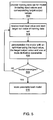
- Figure 5 flowcharts one embodiment of a method for parameterizing a steady state model. More specifically, the method of Figure 5 relates to parameterization of a compact empirical model using derivative constraints and an optimizer.
- system may also refer to a process.
- the method described is exemplary, and that in various embodiments, two or more of the steps shown may be performed concurrently, in a different order than shown, or may be omitted. Additional steps may also be performed as desired.
- in-situ hydrocarbon reservoir example of Figure 4 is used to illustrates various portions of the method, although it is noted that the methods described herein are broadly applicable in other fields and domains, as well, such as, for example, engineering, hydrocarbon, e.g., oil or gas, production, chemical processing, e-commerce, finance, stock analysis, and manufacturing, among others.
- a typical reservoir engineering problem is to determine the injection rates that maximize field production.
- a rigorous simulation model is typically fit to field data in what is known as a "history match". In prior art approaches, a man-year or more may be spent parameterizing or tuning the model so that it replicates what the oil field has done historically.
- the reservoir engineers After a large fraction of the project budget is used up, e.g., 85%, the reservoir engineers typically make 15 or 20 runs of the simulation and then make their best guess for the injection rates.
- the use of compact models may dramatically reduce the time needed to parameterize the model, as described in detail below.
- a training data set may be provided, where the training data set includes a plurality of input values or vectors u and a plurality of target output values y.
- the training data set is preferably representative of the operation of the system.
- the training data set may include historical data, e.g., input and output data from past operation and/or measurements of the system, and/or synthesized data.
- the input values u may represent injection rates and/or injection cell pressures for injection wells in the reservoir
- the target output values y may represent production rates for production wells of the reservoir.
- a next at least one input value u i of the plurality of input values u and a next target output value y i of the plurality of target output values y may be received, as indicated.
- the method may select a next set of input/output value pairs from the training data set for use in parameterizing the model.
- target outputs of the model represented by y
- actual model outputs represented herein by the term y ⁇ i , e.g., y-hat i or y-caret i .
- an optimizer may be used to parameterize the model with a predetermined algorithm using u i , y i , and one or more derivative constraints.
- the one or more derivative constraints are preferably imposed to constrain relationships between the at least one input value u i and a resulting model output value y ⁇ i .
- parameterizing the model may include using an optimizer to perform constrained optimization on the plurality of model parameters to satisfy an objective function ⁇ subject to the derivative constraints.
- the objective function may include minimizing an error between the model output value y ⁇ i (resulting from at least one input value u i ) and the target output value y i .
- the objective function may be defined for each input value/target output value pair, and the optimizer used to determine parameters (coefficients) for the model that minimize the error subject to the derivative constraints.
- a first at least one input value u 0 may be input to the model, where the model is characterized by initial parameter values p 0 , resulting in a first model output value y ⁇ 0 .
- the error indicates the degree to which the model does not display the target behavior, e.g., the degree to which the model coefficients are incorrect.
- a second at least one input value u 1 may then be input to the model, where the model is now characterized by the new parameter values p 1 , resulting in a second model output value y ⁇ 1 .
- This computed slope may then be used to increment p 1 , e.g., to compute ⁇ p 1 , giving p 2 , and so on, where the calculation of each ⁇ p i is performed subject to the derivative constraints.
- This process may be repeated until the parameters converge, i.e., until the model output substantially matches the target output.
- each set or pair of model input/output values, u i /y i comprises data for the system or process at a respective time.
- the set of training data u/y may comprise system or process data spanning a specified duration, e.g., 6 months of logged hydrocarbon reservoir data.
- the model includes a model function
- the one or more derivative constraints include upper and/or lower bounds on one or more model function derivatives.
- the one or more derivative constraints may include estimated allowable ranges for one or more derivatives of the model function.
- the one or more model function derivatives may include one or more of: a first order derivative of the model function, a second order derivative of the model function, and a third order derivative of the model function.
- the one or more model function derivatives also include one or more fourth or higher order derivatives of the model function.
- the one or more model function derivatives may include a zeroth or higher order derivative of the model function, where the zeroth order derivative refers to the model function itself.
- the model function itself may be a constraint, for example, by enforcing the relationships between the input values u i and the target output values y i , although in some embodiments, this constraint may be imposed implicitly or as a consequence of the optimization process.
- At least one of the upper and/or lower bounds may be a constant. In another embodiment, at least one of the upper and/or lower bounds may be a function. In a preferred embodiment, the model function has no cross-terms, with the result that the derivatives of the model function have no cross-terms.
- a determination may be made as to whether the model parameters have converged, e.g., whether the model has converged, and if not, then the method may proceed back to 504, where a next at least one input value u i+1 /target output value y i+1 may be selected, and the process repeated, as indicated.
- the receiving of 504 and the parameterizing using the optimizer of 506 may be performed iteratively to generate a parameterized model.
- the parameterization process may be iteratively performed to determine parameters in a rigorous simulation model.
- the receiving and parameterizing for each at least one input value u i and each target output value y i of the training data set may be performed two or more times.
- the receiving and parameterizing for each at least one input value u i and each target output value y i of the training data set may be performed until the model parameters converge.
- parameterization may be performed using an optimization algorithm that allows inequality constraints on functions of the model parameters or variables.
- the model may be a multiple input-single output (MISO) model, where the model function accepts an input vector, e.g., u and generates a single output value y, as is the case in equation (6) above.
- MISO multiple input-single output
- a plurality of MISO models may be used to model the system or process, where the set of MISO models compose an aggregate model of the system or process.
- the providing, receiving, parameterizing, and iteratively performing described above may be performed for each of a plurality of models, wherein the plurality of models compose an aggregate model of the system.
- each of the plurality of models has a respective model function, where each model function preferably has no cross-terms, although embodiments with cross-terms are also contemplated.
- Each MISO model may represent a respective aspect of the system or process, e.g., in the hydrocarbon reservoir example, each injection well and/or each production well, may have an associated MISO model, or even multiple MISO models, representing the behavior of that respective well.
- providing a training data set comprising a plurality of input values u and a plurality of target output values y for each of said plurality of models may include providing a training data set comprising a plurality of input vectors u and a plurality of target output vectors y , where each input vector u i includes respective input values for each of the plurality of models, and thus each input vector u i is an input vector for the aggregate model.
- each target output vector y may include respective target output values for each of the plurality of models, where each target output vector y is a target output vector for the aggregate model.
- the aggregate model may operate to generate a resulting model output vector y ⁇ i , comprising respective output values for each of the plurality of models.
- the resulting parameterized model (the single MISO model and/or the aggregate model) may then be stored in a memory medium, as indicated in 510, and may be usable to analyze the system.
- the model may be optimized to determine operational parameters of the system for optimal performance of the system, as described below with reference to Figure 6.
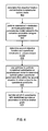
- Figure 6 presents a method for generating and using the parameterized model of Figure 5, according to one embodiment.
- the method described is exemplary, and in various embodiments, two or more of the steps shown may be performed concurrently, in a different order than shown, or may be omitted. Additional steps may also be performed as desired. Note that portions of the method are substantially described above with reference to Figure 5, the descriptions may be abbreviated.
- a first objective function and derivative constraints are determined for the system model, as was described in detail above with reference to Figure 5.
- constrained optimization may be performed with an optimizer on the model parameters to parameterize the model (satisfy the first objective function) subject to the derivative constraints, as described in detail above.
- a second objective function may be determined, where the second objective function represents a desired behavior of the system.
- operational constraints may optionally be determined that reflect bounds or limitations on the operation or behavior of the system.
- the second objective function may be to maximize profits, which in the in-situ reservoir example, may be related to the difference between the cost of the injected materials and the value of the hydrocarbon products produced.
- the operational constraints may include mass balancing, injection pressure limits, and so forth.
- the optimizer and the parameterized model may be used to determine operation of the system that substantially satisfies the second objective function, optionally subject to the operational constraints. Said another way, the optimizer and the parameterized model may then be used to determine operational parameters for the system that attempt to satisfy the second objective function subject to the operational constraints, as is well known in the art. For example, in one embodiment, using the optimizer and the parameterized model to determine operation of the system may include determining one or more operational inputs for the system, where the one or more operational inputs and one or more resulting operational outputs for the system substantially satisfy the second objective function.
- operational constraints may be imposed during the optimization process such that the determined operation of the system substantially satisfies the second objective function subject to one or more operational constraints.
- the optimizer may be used to determine injection rates and/or injection cell pressures for the injection wells that maximize profits, e.g., by maximizing oil production, subject to operational constraints on the system.
- the system may be operated in accordance with the determined operational parameters to achieve desired goals.
- the optimal operational parameters determined with the optimizer and the parameterized model may be used to operate the system.
- this may include executing the optimized (and parameterized) model using input data related to operating conditions of the system to determine the operational parameters needed to produce the desired results, then operating the system using the operational parameters.
- the parameterized model may be executed to generate resultant data, and the system may be operated in accordance with the resultant data to achieve desired results.
- the parameterized model may be executed on a computer to generate data which may be used to operate the system in a substantially optimal manner.
- the model may represent operations related to production of the hydrocarbon from the reservoir.
- the injection wells of the reservoir may be operated using the determined injection rates and/or injection cell pressures that may result in increased oil production and/or profitability.
- various embodiments of the above method may be used to determine operation of the system that substantially satisfies the second objective function subject to one or more operational constraints, i.e., to determine operational parameters for the system for various goals.
- the optimizer and the parameterized model may be used to determine a combination of injection rates that maximizes production within constraints of injection rate and injector cell pressure, to determine operation of the system for secondary and/or tertiary recovery, to determine one or more completion depths for one or more wells, i.e., where to let the oil enter the wellbore, to determine one or more locations for drilling or shutting in wells, and to determine one or more rates of stimulant injection to maximize production, among others.
- the optimization problem may first be defined: inputs (u), outputs (y), objective function, and constraints. Then, from engineering knowledge, the allowable ranges on the first, second, and third derivatives may be estimated: min ⁇ ⁇ y i l ⁇ u j ⁇ max min ⁇ 2 y i / ⁇ u 2 j ⁇ max min ⁇ 3 y i / ⁇ u 3 j ⁇ max
- cross derivatives e.g., ⁇ 2 y i / ⁇ u j ⁇ u k
- the models are built MISO, and cross derivatives are allowed.
- the models may be MISO, but cross-derivatives may be disallowed or ignored.
- the third derivative ranges will generally be quite small, e.g., close to zero.
- the first-order derivative(s) of the model function may include inter-well transmissibilities and/or production indices;
- the second-order derivative(s) of the model function may include curvature for the inter-well transmissibilities and/or production indices;
- the third-order derivative(s) of the model function may include a rate of curvature change for the inter-well transmissibilities and/or production indices.
- scaling data may be selected.
- the scaling data sets the "zeroth" derivatives of the model, i.e., determines the actual range for the model function(s). If data are available from a simulation of the process, a design of experiments method may be used to select the scaling data and make simulation runs to generate it.
- An optimization algorithm e.g., gradient descent, sequential quadratic program, etc.
- the various inequality constraints may be entered, an objective function determined that penalizes the model for errors in its outputs, and an optimization sequence executed, where the optimizer uses the scaling data as inputs to the model, and uses the model outputs to calculate objective function errors.
- the optimization algorithm may then update the model parameters to reduce the errors within parameter derivative constraints. As the model behavior converges the "best fit" set of model parameters may be produced.
- the parameterized model may then be used to solve the original optimization problem posed initially, e.g., using an optimizer. For example, the parameterized model may be executed to generate resultant data, and the system operated in accordance with the resultant data to achieve desired results.
- DCP derivative-constrained parameterization
- a rigorous simulation model may not be required in that a compact empirical model with derivative constraints may accurately capture salient aspects of the system behavior; 2) the data required already exists, i.e., data requirements for using the compact empirical model with derivative constraints are substantially less (e.g., perhaps by a factor of 100) than most prior art approaches, and in many cases the required information is readily available, e.g., from reservoir well inspections (e.g., pressures and flows), engineering data and knowledge (e.g., permeability plots), etc.; 3) engineering the model may take weeks instead of months, due to the simplicity of the model and its reduced data requirements; and finally, 4) the derivatives constraints are intuitive.
- reservoir well inspections e.g., pressures and flows
- engineering data and knowledge e.g., permeability plots
- the derivative constraints and behaviors represent easily understood phenomena related to the modeled system, and thus may generally be specified in a relatively straightforward manner.
- the first derivatives are known as inter-well transmissibilities and production indices.
- the second derivatives indicate how much curvature is allowed, and the third derivatives indicate how fast the curvature can change.
- optimization techniques may be used to both parameterize the system model(s), i.e., by optimizing the model parameters to fit the training data subject to derivative constraints, and to optimize operation of the modeled system, i.e., by optimizing operational system parameters, for example, to meet a production or business objective.
- the two optimization processes are preferably separate and distinct from one another.
- Various embodiments further include receiving or storing instructions and/or data implemented in accordance with the foregoing description upon a carrier medium.
- Suitable carrier media include a memory medium as described above, as well as signals such as electrical, electromagnetic, or digital signals, conveyed via a communication medium such as networks and/or a wireless link.
Landscapes
- Life Sciences & Earth Sciences (AREA)
- Engineering & Computer Science (AREA)
- Geology (AREA)
- Mining & Mineral Resources (AREA)
- Physics & Mathematics (AREA)
- Environmental & Geological Engineering (AREA)
- Fluid Mechanics (AREA)
- General Life Sciences & Earth Sciences (AREA)
- Geochemistry & Mineralogy (AREA)
- Feedback Control In General (AREA)
- Management, Administration, Business Operations System, And Electronic Commerce (AREA)
Applications Claiming Priority (2)
| Application Number | Priority Date | Filing Date | Title |
|---|---|---|---|
| US10/350,838 US7899657B2 (en) | 2003-01-24 | 2003-01-24 | Modeling in-situ reservoirs with derivative constraints |
| US350838 | 2003-01-24 |
Publications (3)
| Publication Number | Publication Date |
|---|---|
| EP1441238A2 true EP1441238A2 (de) | 2004-07-28 |
| EP1441238A3 EP1441238A3 (de) | 2005-05-25 |
| EP1441238B1 EP1441238B1 (de) | 2007-03-07 |
Family
ID=32594953
Family Applications (1)
| Application Number | Title | Priority Date | Filing Date |
|---|---|---|---|
| EP04001565A Expired - Lifetime EP1441238B1 (de) | 2003-01-24 | 2004-01-26 | Modellierung von in-situ Ölreservoiren mittels Ableitungsbeschränkungen |
Country Status (3)
| Country | Link |
|---|---|
| US (1) | US7899657B2 (de) |
| EP (1) | EP1441238B1 (de) |
| DE (1) | DE602004005085T2 (de) |
Cited By (4)
| Publication number | Priority date | Publication date | Assignee | Title |
|---|---|---|---|---|
| EP1630348A1 (de) * | 2004-08-30 | 2006-03-01 | Institut Français du Pétrole | Verfahren zur Modellierung der Ölgewinnung aus einer unterirdischen Formation |
| WO2007060446A1 (en) * | 2005-11-26 | 2007-05-31 | The University Court Of The University Of Edinburgh | Improvements in and relating to hydrocarbon recovery from a hydrocarbon reservoir |
| EP2465073A4 (de) * | 2009-08-12 | 2014-09-03 | Exxonmobil Upstream Res Co | Optimierte richtlinien für bohrlochmanagement |
| US8849623B2 (en) | 2008-12-16 | 2014-09-30 | Exxonmobil Upstream Research Company | Systems and methods for reservoir development and management optimization |
Families Citing this family (43)
| Publication number | Priority date | Publication date | Assignee | Title |
|---|---|---|---|---|
| US6853921B2 (en) | 1999-07-20 | 2005-02-08 | Halliburton Energy Services, Inc. | System and method for real time reservoir management |
| US7584165B2 (en) * | 2003-01-30 | 2009-09-01 | Landmark Graphics Corporation | Support apparatus, method and system for real time operations and maintenance |
| FR2886742B1 (fr) * | 2005-06-02 | 2007-07-27 | Inst Francais Du Petrole | Methode de changement d'echelle des permeabilites absolues pour construire un modele de simulation d'ecoulement |
| EP1999492A4 (de) * | 2006-01-20 | 2011-05-18 | Landmark Graphics Corp | Dynamisches produktionsverwaltungssystem |
| FR2919932B1 (fr) * | 2007-08-06 | 2009-12-04 | Inst Francais Du Petrole | Methode pour evaluer un schema de production d'un gissement souterrain en tenant compte des incertitudes |
| CN101842756A (zh) * | 2007-08-14 | 2010-09-22 | 国际壳牌研究有限公司 | 用于化工厂或精炼厂的连续、在线监视的系统与方法 |
| US20090076632A1 (en) * | 2007-09-18 | 2009-03-19 | Groundswell Technologies, Inc. | Integrated resource monitoring system with interactive logic control |
| US8892221B2 (en) * | 2007-09-18 | 2014-11-18 | Groundswell Technologies, Inc. | Integrated resource monitoring system with interactive logic control for well water extraction |
| US20110161133A1 (en) * | 2007-09-29 | 2011-06-30 | Schlumberger Technology Corporation | Planning and Performing Drilling Operations |
| US8103493B2 (en) * | 2007-09-29 | 2012-01-24 | Schlumberger Technology Corporation | System and method for performing oilfield operations |
| CA2705277C (en) * | 2007-12-18 | 2017-01-17 | Exxonmobil Upstream Research Company | Determining connectivity architecture in 2-d and 3-d heterogeneous data |
| EP2232406A4 (de) | 2007-12-21 | 2017-10-18 | Exxonmobil Upstream Research Company | Verfahren und vorrichtung zum analysieren dreidimensionaler daten |
| EP2235566A1 (de) * | 2008-01-22 | 2010-10-06 | Exxonmobil Upstream Research Company | Dynamische konnektivitätsanalyse |
| WO2009114211A1 (en) | 2008-03-10 | 2009-09-17 | Exxonmobil Upstream Research Company | Method for determing distinct alternative paths between two object sets in 2-d and 3-d heterogeneous data |
| US9733388B2 (en) | 2008-05-05 | 2017-08-15 | Exxonmobil Upstream Research Company | Systems and methods for connectivity analysis using functional objects |
| US20110067871A1 (en) * | 2008-05-22 | 2011-03-24 | Burdette Jason A | Methods For Regulating Flow In Multi-Zone Intervals |
| US9228415B2 (en) | 2008-10-06 | 2016-01-05 | Schlumberger Technology Corporation | Multidimensional data repository for modeling oilfield operations |
| US8352228B2 (en) * | 2008-12-23 | 2013-01-08 | Exxonmobil Upstream Research Company | Method for predicting petroleum expulsion |
| US9552462B2 (en) * | 2008-12-23 | 2017-01-24 | Exxonmobil Upstream Research Company | Method for predicting composition of petroleum |
| EP2406663A1 (de) | 2009-03-13 | 2012-01-18 | Exxonmobil Upstream Research Company | Verfahren zur vorhersage von fluidströmung |
| AU2010308495A1 (en) | 2009-10-20 | 2012-05-10 | Exxonmobil Upstream Research Company | Method for quantitatively assessing connectivity for well pairs at varying frequencies |
| CA2785569A1 (en) * | 2010-02-02 | 2011-08-11 | Hector Klie | Multilevel percolation aggregation solver for petroleum reservoir simulations |
| US9594186B2 (en) | 2010-02-12 | 2017-03-14 | Exxonmobil Upstream Research Company | Method and system for partitioning parallel simulation models |
| EP2545461A4 (de) | 2010-03-12 | 2017-09-27 | Exxonmobil Upstream Research Company | Dynamische gruppierung von domain-objekten über intelligente gruppen |
| CA2805446C (en) * | 2010-07-29 | 2016-08-16 | Exxonmobil Upstream Research Company | Methods and systems for machine-learning based simulation of flow |
| EP2668641B1 (de) | 2011-01-26 | 2020-04-15 | Exxonmobil Upstream Research Company | Verfahren zur analyse eines reservoirkompartiments mit topologischer struktur bei 3d-erdmodellen |
| DE102011084473B4 (de) * | 2011-10-13 | 2022-06-23 | Vitesco Technologies GmbH | Verfahren zum Symmetrieren von Speicherzellen einer Speichervorrichtung und Speichersystem zum Durchführen des Verfahrens |
| US20130332120A1 (en) * | 2012-06-06 | 2013-12-12 | University Of Southern California | System and method for aggregating reservoir connectivities |
| US8821199B2 (en) | 2012-07-25 | 2014-09-02 | Targus Group International, Inc. | Multi-prong power tip adaptor |
| EP3008281A2 (de) | 2013-06-10 | 2016-04-20 | Exxonmobil Upstream Research Company | Interaktive planung einer bohrstelle |
| US9085958B2 (en) * | 2013-09-19 | 2015-07-21 | Sas Institute Inc. | Control variable determination to maximize a drilling rate of penetration |
| US9864098B2 (en) | 2013-09-30 | 2018-01-09 | Exxonmobil Upstream Research Company | Method and system of interactive drill center and well planning evaluation and optimization |
| US9163497B2 (en) | 2013-10-22 | 2015-10-20 | Sas Institute Inc. | Fluid flow back prediction |
| CA3072107C (en) | 2017-09-28 | 2022-08-30 | Chevron U.S.A. Inc. | Systems and methods for estimating reservoir productivity as a function of depth in a subsurface volume of interest |
| CA3076522C (en) * | 2017-09-28 | 2023-08-22 | Chevron U.S.A. Inc. | Systems and methods for estimating reservoir productivity as a function of position in a subsurface volume of interest |
| US11423197B2 (en) * | 2017-09-28 | 2022-08-23 | Chevron U.S.A. Inc. | Systems and methods for estimating a well design reservoir productivity as a function of position in a subsurface volume of interest based on a reservoir productivity parameter |
| CA3076523C (en) | 2017-09-28 | 2023-04-04 | Chevron, U.S.A. | Systems and methods for estimating a likelihood of reservoir productivity as a function of position in a subsurface volume of interest |
| WO2020172268A1 (en) * | 2019-02-20 | 2020-08-27 | Chevron U.S.A. Inc. | Systems and methods for estimating a well design reservoir productivity as a function of position in a subsurface volume of interest based on a reservoir productivity parameter |
| US11371336B2 (en) | 2019-09-19 | 2022-06-28 | Chevron U.S.A. Inc. | Systems and methods for estimating refined reservoir productivity values as a function of position in a subsurface volume of interest |
| US11668854B2 (en) | 2019-10-15 | 2023-06-06 | Chevron U.S.A. Inc. | Forecasting hydrocarbon production |
| US11480709B2 (en) * | 2019-10-21 | 2022-10-25 | Chevron U.S.A. Inc. | Systems and methods for predicting hydrocarbon production and assessing prediction uncertainty |
| US11055639B1 (en) * | 2020-04-28 | 2021-07-06 | Sas Institute Inc. | Optimizing manufacturing processes using one or more machine learning models |
| US11193370B1 (en) | 2020-06-05 | 2021-12-07 | Saudi Arabian Oil Company | Systems and methods for transient testing of hydrocarbon wells |
Family Cites Families (15)
| Publication number | Priority date | Publication date | Assignee | Title |
|---|---|---|---|---|
| US5444619A (en) * | 1993-09-27 | 1995-08-22 | Schlumberger Technology Corporation | System and method of predicting reservoir properties |
| US6278899B1 (en) * | 1996-05-06 | 2001-08-21 | Pavilion Technologies, Inc. | Method for on-line optimization of a plant |
| US6047221A (en) * | 1997-10-03 | 2000-04-04 | Pavilion Technologies, Inc. | Method for steady-state identification based upon identified dynamics |
| US7058617B1 (en) * | 1996-05-06 | 2006-06-06 | Pavilion Technologies, Inc. | Method and apparatus for training a system model with gain constraints |
| US6381504B1 (en) * | 1996-05-06 | 2002-04-30 | Pavilion Technologies, Inc. | Method for optimizing a plant with multiple inputs |
| US5905657A (en) * | 1996-12-19 | 1999-05-18 | Schlumberger Technology Corporation | Performing geoscience interpretation with simulated data |
| US6434435B1 (en) * | 1997-02-21 | 2002-08-13 | Baker Hughes Incorporated | Application of adaptive object-oriented optimization software to an automatic optimization oilfield hydrocarbon production management system |
| US6002985A (en) * | 1997-05-06 | 1999-12-14 | Halliburton Energy Services, Inc. | Method of controlling development of an oil or gas reservoir |
| US6236894B1 (en) * | 1997-12-19 | 2001-05-22 | Atlantic Richfield Company | Petroleum production optimization utilizing adaptive network and genetic algorithm techniques |
| US6101447A (en) * | 1998-02-12 | 2000-08-08 | Schlumberger Technology Corporation | Oil and gas reservoir production analysis apparatus and method |
| AU3229900A (en) | 1999-02-12 | 2000-08-29 | Prange, Michael | Uncertainty constrained subsurface modeling |
| DE60102242T2 (de) * | 2000-06-29 | 2005-01-27 | Aspen Technology, Inc., Cambridge | Rechnerverfahren und gerät zur beschränkung einer nicht-linearen gleichungsnäherung eines empirischen prozesses |
| US6901391B2 (en) * | 2001-03-21 | 2005-05-31 | Halliburton Energy Services, Inc. | Field/reservoir optimization utilizing neural networks |
| FR2823877B1 (fr) * | 2001-04-19 | 2004-12-24 | Inst Francais Du Petrole | Methode pour contraindre par des donnees dynamiques de production un modele fin representatif de la repartition dans le gisement d'une grandeur physique caracteristique de la structure du sous-sol |
| US7424415B2 (en) | 2001-06-06 | 2008-09-09 | Schlumberger Technology Corporation | Automated system for modeling faulted multi-valued horizons |
-
2003
- 2003-01-24 US US10/350,838 patent/US7899657B2/en active Active
-
2004
- 2004-01-26 DE DE602004005085T patent/DE602004005085T2/de not_active Expired - Lifetime
- 2004-01-26 EP EP04001565A patent/EP1441238B1/de not_active Expired - Lifetime
Cited By (7)
| Publication number | Priority date | Publication date | Assignee | Title |
|---|---|---|---|---|
| EP1630348A1 (de) * | 2004-08-30 | 2006-03-01 | Institut Français du Pétrole | Verfahren zur Modellierung der Ölgewinnung aus einer unterirdischen Formation |
| FR2874706A1 (fr) * | 2004-08-30 | 2006-03-03 | Inst Francais Du Petrole | Methode de modelisation de la production d'un gisement petrolier |
| US7788074B2 (en) | 2004-08-30 | 2010-08-31 | Institut Francais Du Petrole | Method of modelling the production of an oil reservoir |
| WO2007060446A1 (en) * | 2005-11-26 | 2007-05-31 | The University Court Of The University Of Edinburgh | Improvements in and relating to hydrocarbon recovery from a hydrocarbon reservoir |
| EA012093B1 (ru) * | 2005-11-26 | 2009-08-28 | Де Юниверсити Корт Ов Де Юниверсити Ов Эдинбург | Усовершенствования извлечения углеводородов из коллектора углеводородов |
| US8849623B2 (en) | 2008-12-16 | 2014-09-30 | Exxonmobil Upstream Research Company | Systems and methods for reservoir development and management optimization |
| EP2465073A4 (de) * | 2009-08-12 | 2014-09-03 | Exxonmobil Upstream Res Co | Optimierte richtlinien für bohrlochmanagement |
Also Published As
| Publication number | Publication date |
|---|---|
| US7899657B2 (en) | 2011-03-01 |
| US20040148147A1 (en) | 2004-07-29 |
| EP1441238B1 (de) | 2007-03-07 |
| DE602004005085T2 (de) | 2007-11-22 |
| EP1441238A3 (de) | 2005-05-25 |
| DE602004005085D1 (de) | 2007-04-19 |
Similar Documents
| Publication | Publication Date | Title |
|---|---|---|
| US7899657B2 (en) | Modeling in-situ reservoirs with derivative constraints | |
| EP1441268A1 (de) | Parametrierung eines Modells im Stationären Zustand mit Hilfe von Ableitungs-Nebenbediengungen | |
| AU2008338406B2 (en) | Systems and methods for optimization of real time production operations | |
| Zangl et al. | Proxy modeling in production optimization | |
| Guo et al. | Integration of support vector regression with distributed Gauss-Newton optimization method and its applications to the uncertainty assessment of unconventional assets | |
| Saputelli et al. | Best practices and lessons learned after 10 years of digital oilfield (DOF) implementations | |
| Sarma et al. | Redistribution of steam injection in heavy oil reservoir management to improve EOR economics, powered by a unique integration of reservoir physics and machine learning | |
| WO2011019421A1 (en) | Optimizing well management policy | |
| Onita et al. | Economic impact of novel petrophysical decision-making in oil rim reservoir development: A theoretical approach | |
| Sankaran et al. | Data analytics in reservoir engineering | |
| Schiozer et al. | Model-based life-cycle optimization for field development and management integrated with production facilities | |
| Bratvold et al. | I would rather be vaguely right than precisely wrong: A new approach to decision making in the petroleum exploration and production industry | |
| Howell et al. | From Reservoir Through Process, From Today to Tomorrow—The Integrated Asset Model | |
| Choudhary et al. | Application of global optimization methods for history matching and probabilistic forecasting—case studies | |
| de Souza Jr et al. | Controlled time series forecasting for oil reservoir management | |
| Emmanoulopoulos et al. | To trade or not to trade: An agentic approach to estimating market risk improves trading decisions | |
| Holdaway | Predictive Analytics: Development and Deployment of Upstream Data Driven Models | |
| Esmaiel et al. | Optimization of the WAG process under uncertainty in a smart wells environment: Utility theory approach | |
| Sun | A scenario management platform that incorporates statistic and simulation for unconventional field development | |
| Rezaeian et al. | Optimization of an integrated reservoir-production system using polynomial chaos expansion and sobol sensitivity analysis | |
| Guzman Piedra | Modeling and Optimizing a Mature Field Operated by WAG Injection Using Integrated Machine Learning and Reservoir Physics | |
| Siraj | Reducing the effect of uncertainty in robust optimization for oil recovery | |
| Alsaeedi et al. | Integrated Digital Production Platform with the Reservoir Dynamic Models for a Giant Gas Condensate Reservoir in Real Time | |
| Gladchenko et al. | Multi-Engine AI Tool for Oil Field Development Plan Optimization | |
| Hørsholt | Operational optimization of oil reservoirs in the danish north sea |
Legal Events
| Date | Code | Title | Description |
|---|---|---|---|
| PUAI | Public reference made under article 153(3) epc to a published international application that has entered the european phase |
Free format text: ORIGINAL CODE: 0009012 |
|
| AK | Designated contracting states |
Kind code of ref document: A2 Designated state(s): AT BE BG CH CY CZ DE DK EE ES FI FR GB GR HU IE IT LI LU MC NL PT RO SE SI SK TR |
|
| AX | Request for extension of the european patent |
Extension state: AL LT LV MK |
|
| PUAL | Search report despatched |
Free format text: ORIGINAL CODE: 0009013 |
|
| RIC1 | Information provided on ipc code assigned before grant |
Ipc: 7E 21B 49/00 B Ipc: 7G 01V 1/30 A |
|
| AK | Designated contracting states |
Kind code of ref document: A3 Designated state(s): AT BE BG CH CY CZ DE DK EE ES FI FR GB GR HU IE IT LI LU MC NL PT RO SE SI SK TR |
|
| AX | Request for extension of the european patent |
Extension state: AL LT LV MK |
|
| 17P | Request for examination filed |
Effective date: 20050919 |
|
| GRAP | Despatch of communication of intention to grant a patent |
Free format text: ORIGINAL CODE: EPIDOSNIGR1 |
|
| AKX | Designation fees paid |
Designated state(s): BE DE FR GB LU NL |
|
| GRAS | Grant fee paid |
Free format text: ORIGINAL CODE: EPIDOSNIGR3 |
|
| RAP1 | Party data changed (applicant data changed or rights of an application transferred) |
Owner name: PAVILION TECHNOLOGIES, INC. |
|
| GRAA | (expected) grant |
Free format text: ORIGINAL CODE: 0009210 |
|
| AK | Designated contracting states |
Kind code of ref document: B1 Designated state(s): BE DE FR GB LU NL |
|
| REG | Reference to a national code |
Ref country code: GB Ref legal event code: FG4D |
|
| REF | Corresponds to: |
Ref document number: 602004005085 Country of ref document: DE Date of ref document: 20070419 Kind code of ref document: P |
|
| ET | Fr: translation filed | ||
| PLBE | No opposition filed within time limit |
Free format text: ORIGINAL CODE: 0009261 |
|
| STAA | Information on the status of an ep patent application or granted ep patent |
Free format text: STATUS: NO OPPOSITION FILED WITHIN TIME LIMIT |
|
| 26N | No opposition filed |
Effective date: 20071210 |
|
| PGFP | Annual fee paid to national office [announced via postgrant information from national office to epo] |
Ref country code: LU Payment date: 20110201 Year of fee payment: 8 Ref country code: NL Payment date: 20110128 Year of fee payment: 8 Ref country code: FR Payment date: 20110301 Year of fee payment: 8 Ref country code: DE Payment date: 20110127 Year of fee payment: 8 |
|
| PGFP | Annual fee paid to national office [announced via postgrant information from national office to epo] |
Ref country code: BE Payment date: 20110124 Year of fee payment: 8 |
|
| PGFP | Annual fee paid to national office [announced via postgrant information from national office to epo] |
Ref country code: GB Payment date: 20110125 Year of fee payment: 8 |
|
| BERE | Be: lapsed |
Owner name: PAVILION TECHNOLOGIES, INC. Effective date: 20120131 |
|
| REG | Reference to a national code |
Ref country code: NL Ref legal event code: V1 Effective date: 20120801 |
|
| GBPC | Gb: european patent ceased through non-payment of renewal fee |
Effective date: 20120126 |
|
| REG | Reference to a national code |
Ref country code: FR Ref legal event code: ST Effective date: 20120928 |
|
| PG25 | Lapsed in a contracting state [announced via postgrant information from national office to epo] |
Ref country code: GB Free format text: LAPSE BECAUSE OF NON-PAYMENT OF DUE FEES Effective date: 20120126 Ref country code: DE Free format text: LAPSE BECAUSE OF NON-PAYMENT OF DUE FEES Effective date: 20120801 |
|
| REG | Reference to a national code |
Ref country code: DE Ref legal event code: R119 Ref document number: 602004005085 Country of ref document: DE Effective date: 20120801 |
|
| PG25 | Lapsed in a contracting state [announced via postgrant information from national office to epo] |
Ref country code: BE Free format text: LAPSE BECAUSE OF NON-PAYMENT OF DUE FEES Effective date: 20120131 Ref country code: FR Free format text: LAPSE BECAUSE OF NON-PAYMENT OF DUE FEES Effective date: 20120131 |
|
| PG25 | Lapsed in a contracting state [announced via postgrant information from national office to epo] |
Ref country code: NL Free format text: LAPSE BECAUSE OF NON-PAYMENT OF DUE FEES Effective date: 20120801 |
|
| PG25 | Lapsed in a contracting state [announced via postgrant information from national office to epo] |
Ref country code: LU Free format text: LAPSE BECAUSE OF NON-PAYMENT OF DUE FEES Effective date: 20120126 |