EP1626317B1 - Procédé de mise au point d'un modèle non-lineaire ,stationaire ou dynamique de variable de commande pour engin de construction - Google Patents
Procédé de mise au point d'un modèle non-lineaire ,stationaire ou dynamique de variable de commande pour engin de construction Download PDFInfo
- Publication number
- EP1626317B1 EP1626317B1 EP05450114A EP05450114A EP1626317B1 EP 1626317 B1 EP1626317 B1 EP 1626317B1 EP 05450114 A EP05450114 A EP 05450114A EP 05450114 A EP05450114 A EP 05450114A EP 1626317 B1 EP1626317 B1 EP 1626317B1
- Authority
- EP
- European Patent Office
- Prior art keywords
- model
- function
- weighting function
- value
- weighting
- Prior art date
- Legal status (The legal status is an assumption and is not a legal conclusion. Google has not performed a legal analysis and makes no representation as to the accuracy of the status listed.)
- Expired - Lifetime
Links
Images




Classifications
-
- G—PHYSICS
- G05—CONTROLLING; REGULATING
- G05B—CONTROL OR REGULATING SYSTEMS IN GENERAL; FUNCTIONAL ELEMENTS OF SUCH SYSTEMS; MONITORING OR TESTING ARRANGEMENTS FOR SUCH SYSTEMS OR ELEMENTS
- G05B13/00—Adaptive control systems, i.e. systems automatically adjusting themselves to have a performance which is optimum according to some preassigned criterion
- G05B13/02—Adaptive control systems, i.e. systems automatically adjusting themselves to have a performance which is optimum according to some preassigned criterion electric
- G05B13/0265—Adaptive control systems, i.e. systems automatically adjusting themselves to have a performance which is optimum according to some preassigned criterion electric the criterion being a learning criterion
- G05B13/027—Adaptive control systems, i.e. systems automatically adjusting themselves to have a performance which is optimum according to some preassigned criterion electric the criterion being a learning criterion using neural networks only
-
- G—PHYSICS
- G05—CONTROLLING; REGULATING
- G05B—CONTROL OR REGULATING SYSTEMS IN GENERAL; FUNCTIONAL ELEMENTS OF SUCH SYSTEMS; MONITORING OR TESTING ARRANGEMENTS FOR SUCH SYSTEMS OR ELEMENTS
- G05B13/00—Adaptive control systems, i.e. systems automatically adjusting themselves to have a performance which is optimum according to some preassigned criterion
- G05B13/02—Adaptive control systems, i.e. systems automatically adjusting themselves to have a performance which is optimum according to some preassigned criterion electric
- G05B13/04—Adaptive control systems, i.e. systems automatically adjusting themselves to have a performance which is optimum according to some preassigned criterion electric involving the use of models or simulators
- G05B13/048—Adaptive control systems, i.e. systems automatically adjusting themselves to have a performance which is optimum according to some preassigned criterion electric involving the use of models or simulators using a predictor
-
- G—PHYSICS
- G05—CONTROLLING; REGULATING
- G05B—CONTROL OR REGULATING SYSTEMS IN GENERAL; FUNCTIONAL ELEMENTS OF SUCH SYSTEMS; MONITORING OR TESTING ARRANGEMENTS FOR SUCH SYSTEMS OR ELEMENTS
- G05B17/00—Systems involving the use of models or simulators of said systems
- G05B17/02—Systems involving the use of models or simulators of said systems electric
Definitions
- the invention relates to a method for producing a nonlinear stationary or dynamic model of a work machine, in particular an internal combustion engine or a subsystem thereof, in the entire space of all operating points of the work machine, preferably using neural networks, with one of a set of input variables, for example system parameters, time-differentiated system parameters, time-delayed feedback output variables and / or default values at the respective operating point dependent control variable, which is determined by measurement for a group of operating points from the entire space of operating points of the work machine, wherein at these operating points using a simplified partial model function an output variable is determined per model function, and wherein at any operating point the outputs of each partial model function with an associated weighting function weighted to a Ge velvet output variable for the respective operating point are added together, wherein for all operating points with metrologically determined control variable respectively the difference between the total output and the metrologically determined value of the control variable is determined and in areas of operating points with an absolute value of this difference above a predetermined value another model function is used with a further associated weighting function
- Models of systems or processes are needed for a variety of applications, such as predicting or simulating system behavior to gain a better understanding of the system, improving or optimizing an existing process or designing a new system, or even creating sliders, Fault diagnosis and control systems for real systems based on process models.
- nonlinear systems can have the property of infinite structural diversity compared to linear systems.
- a major requirement of an algorithm for identifying nonlinear systems is therefore that a variety of structurally different systems can be described.
- local model trees are capable of large numbers nonlinear systems and can therefore be used in applications where a high degree of flexibility is required.
- the basic principle of neuro-fuzzy models has been developed more or less independently in several areas such as neural networks, fuzzy logic, statistics and artificial intelligence under a variety of names such as local models network, Takagi-Sugeno fuzzy models or local models.
- the model architecture of the linear neuro-fuzzy submodels represent an excellent approach to integrate several knowledge sources, as they have a good interpretability.
- the Neuro Fuzzy model interpolates local models that are valid in different operating ranges.
- Local Linear Model Tree LLOIMOT
- This algorithm has an outer loop that sets the scopes of the submodels, and an inner loop that determines the parameters of those submodels.
- the areas in which the linear models are valid are not sharply separated but blurred, i. the linear submodels are merged by appropriate weight functions, so-called validity functions. Normally, Gaussian distribution functions are used for this purpose.
- the parameters of the linear submodels are determined using the method of least squares, which has clear advantages over a global parameter estimation.
- the nonlinear model parameters, i. the number and parameters of the weighting functions are determined by an iterative design algorithm to avoid the use of nonlinear optimization techniques.
- Local Model Trees One of the main strengths of Local Model Trees is that the premise (ie weighting function) and the impact (ie linear submodel) do not have to be dependent on identical variables. Thus, the "bane of dimensionality" can be avoided by incorporating prior knowledge of the process.
- Another advantage of Local Model Trees is that they are designed to automatically adapt to the complexity of the problem in a highly efficient way. Those areas of the input space where the structure of the nonlinearity is complex are subdivided into many subareas so that they can be represented sufficiently by submodels.
- the LOLIMOT algorithm was designed to systematically halve areas of the input space. Submodels that do not fit well enough will therefore be replaced by two or more smaller models, with the expectation that they better reflect the nonlinear objective function within their scope.
- the main drawback of this approach is that this strategy is more or less trial-and-error based and therefore requires a lot of unnecessary computing power.
- the area divisions are axis orthogonal, which is why the requirements are often not met by the structure of nonlinearity.
- the number of data for modeling is limited and the distribution in the entrance area is low. This causes a limitation of the tree construction algorithm and results in many submodels being formed where much less would be sufficient. This problem has recently been addressed by fuzzy clustering, but the algorithm is still limited to orthogonal partitioning.
- the object of the present invention was therefore a method of the kind set forth, which is faster, i. with fewer iterations, to an optimal overall model for the control variable of a work machine, in particular an internal combustion engine or a subsystem thereof, and satisfies a statistically justified high prediction quality, so that ultimately there is an overall model, which with very few submodels a very good statistical prediction quality having.
- the optimal determination of the control variable of the working machine should also be possible in the non-measured operating points.
- the invention provides that the steps of determining the difference between the total output of the associated partial model functions and a real value of the control variable at this real operating point and the application of another model function and further weighting function are traversed until the statistically evaluated predictive quality of the overall model has reached a desired value.
- each weighting function has a radially symmetrical function (hyper-ellipsoid) in the n-dimensional space of the operating points
- the isocurves of the weighting function in the space of the operating points represent a closed geometric entity
- the isocurve of the weighting function in the n-dimensional space is preferably a hyper-ellipsoid whose main axes in the space of the operating points have in principle any orientation relative to the coordinate system.
- the best transition between the local submodels can be achieved in that the weighting function is an exponential function of at least one input variable at the respective operating point.
- a first weighting function is provided whose isocurve of a defined weighting value geometrically encloses all real operating points.
- the number of real operating points within the isocurve of a defined weighting value of the weighting function is greater than the number of regressors, preferably by at least a factor of 1.05.
- the alignment and extent of each submodel is optimally adjusted by these measures to the existing training data, with maximum statistical correspondence to the measured data and to the signal / noise ratio, whereby the determination of the local regression parameters is a well conditioned problem.
- this partial model and associated weighting function are removed from the overall model ,
- the error of the model function is kept within the defined isocurves of each weighting function less than 10%.
- the high efficiency of the method according to the invention leads to a significantly better result with simultaneously lower computational effort, fewer submodels and generally better confidence.
- the neural network presented here is able to provide information about its accuracy in the form of confidence intervals.
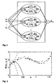
- FIG. 1 schematically the structure of a Local Model Tree
- Fig. 2 shows the "start submodel" using the example of a nonlinear input function
- Fig. 3 is the final situation for the example of Fig. 2
- Fig. 4 shows the finished model for a higher confidence interval
- Fig. 5 contains the same function but with drastically reduced noise
- Fig. 6a is an illustration of an original ellipsoidal weighting function for a 2-dimensional input space
- Fig. 6b shows another weighting function that has cut out a small area from the original weighting function
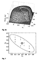
- Fig. 7 shows an example of the placement and alignment of a weighting function over the input space
- Fig. 8 is an example of a nonlinear function over a one-dimensional input space
- Fig. 1 schematically the structure of a Local Model Tree
- Fig. 2 shows the "start submodel" using the example of a nonlinear input function
- Fig. 3 is the final situation for the example of Fig. 2
- Fig. 4 shows the
- FIG. 9 shows the three-dimensional input space with actual measurement data of an internal combustion engine as training data for modeling
- Fig. 10 is the representation of a model for a given constant speed
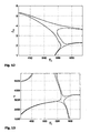
- Fig. 11 the model for a given valve lift, taking FIGS. 12 and 13 the distribution of the weighting functions for the sections of the 10 and FIG. 11 demonstrate
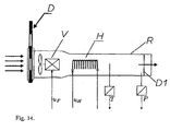
- Fig. 14 shows schematically a test setup for air flow and temperature control
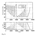
- Fig. 15 shows the excitation signal and the measured output together with the model output for the temperature change
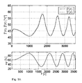
- Fig. 16 shows the model output a special validation signal compared to the measured data from the actual plant Fig. 14 ,
- Fig. 1 shows the structure of a Local Model Tree.
- the total network output value is the sum of all weighted sub -output values ⁇ i : (Equation 4).
- ⁇ i is a vector with the parameters of the submodels and the submodels are generated with u and ⁇ i .
- the model is static if the input vector consists of steady-state variables and becomes dynamic if one or more of the inputs is either the time derivative of a system variable, or if it is the output of one or more sampling steps of a discrete-time system.
- the overall quality of the network output is determined by two different model quality criteria.
- the maximum value of R 2 is 1, which means that the model perfectly emulates all training data.
- R 2 is a suitable model quality value, but if measurement noise is present, optimizing R 2 can easily lead to overfitting.
- each submodel undergoes a final check for its contribution to the overall output value. If it turns out that a model makes only a very small contribution, because it has been largely replaced by other models, this is removed according to a preferred variant of this method from the overall model again.
- Each sub-model roughly consists of two parts: its weighting function ⁇ (u) and its model parameters ⁇ .
- x T ( u ) represents a row vector with regression functions that can be chosen arbitrarily.
- the advantage of the structure in (4) is that ⁇ depends linearly on the parameters ⁇ . Therefore, the method of least squares can be used for their calculation. It remains the determination of suitable regression functions for x T ( u ), which will be discussed in more detail below.
- the training data is represented by dots.
- Figure 2 shows the "start submodel": z i was selected as the center candidate for this example, all data points in the interval u ⁇ [0, 1.7] were selected for the regression.
- the dashed line represents the limits of the 97% confidence interval.
- Fig. 3 shows the final situation: Additional training data has been added until at least 97% of the selected data is within the limits of the 97% confidence interval.
- the resulting weighting function added to the image for clarity ranges from 0.1 to 0.8 and has its maximum at 0.4.
- a greater trust value means greater confidence intervals and subsequently results in a larger expansion of the weighting function.
- you can see that the shape of the nonlinearity has a much greater influence on the model size than in Fig. 3 ,
- Fig. 5 contains the same function f ( x ), but the influence of measurement noise has been drastically reduced. Although the trustworthiness is still 99.99%, the weighting function is now significantly smaller. From these examples it becomes clear that the confidence value is an excellent regularization parameter, which automatically adapts the submodel to the measurement noise of the training data and to the regression factors.
- the vector z i contains the position of the submodel center, as well as the orientation and extent of the weighting function in the input space. With the aid of a shape factor, the flatness of the weighting function can be determined.
- each weighting function is initially a radially symmetric function in the n-dimensional space of the operating points or training data whose isocurve in this n-dimensional space is a closed geometric entity, preferably a hyper-ellipsoid.
- the preferred form is an exponential function with ellipsoidal contours.
- the product in (5) cuts out all subsequent weighting functions from the original function (see Fig. 6 ). This procedure has the following advantage: All subsequent submodels are placed in those areas of the input space where the previous model is insufficient. Equation (5) ensures the dominance of the new submodel in these domains.
- Fig. 6 the following advantage: All subsequent submodels are placed in those areas of the input space where the previous model is insufficient. Equation (5) ensures the dominance of the new submodel in these domains.
- the principal orientation of the new weighting function is therefore determined by [cov (U sel )] -1 , its extent in the input space is controlled by ⁇ . ⁇ is chosen so that ⁇ i remains 0.9 at the data point in U sel farthest from the new center z i . This ensures that enough data points are actually available for parameter estimation.
- ⁇ and ⁇ also serve as further regularization factors for this modeling algorithm.
- the factor ⁇ is directly related to the choice of ⁇ and has only to ensure that the "least squares error problem" is well conditioned as mentioned earlier. Consequently, the confidence values ⁇ and ⁇ are used to parameterize the training algorithm.
- the weighting function is very efficiently adapted to the data in which its principal axes are not necessarily parallel to the axes of the input space of the operating points of the system, but may in principle have any orientation.
- the algorithm does not depend on a favorable choice of the partitioning parameters, but is able to form models that fit very well with the available data.
- the output of each submodel is calculated by the regression model (3).
- Suitable regression functions x T (u) have to be determined.
- the assumption is made that the nonlinear function f (u): R q ⁇ R which is to be approximated, at least twice continuously differentiable at each point u ⁇ U, where U stands for the definition space in which f (u) is to be approximated. If the above assumption holds, then f (u) at each point u ⁇ U can be developed into a Taylor series.
- f (u) can be approximated anywhere in the neighborhood of u t if the submodel is small enough. Depending on the local complexity of f (u) , this would lead to a large number of submodels in areas of strong variability of f (u) and to less large submodels in areas where f (u) is relatively flat. Apart from the residual error of the Taylor series, the algorithm must also handle errors due to measurement noise, so that the actual size of each submodel is affected by both errors.
- c i is a constant offset
- a i denotes a vector with linear parameters
- B i is a lower triangular matrix, which includes the parameters of the quadratic term.
- X a matrix with the regression vectors of all n training data sets:
- X x T u 1 x T u 2 ⁇ ⁇ ⁇ x T u n
- Q i a diagonal matrix consisting of the ⁇ i , evaluated at the training data points:
- Q i ⁇ i u 1 0 ⁇ 0 0 ⁇ i u 2 ⁇ 0 ⁇ ⁇ ⁇ ⁇ 0 0 ⁇ ⁇ i u n
- X contains the same regression functions (or a part thereof) as x (u) in the submodels, e is a white noise vector, with the standard deviation ⁇ n and ⁇ is the vector of the parameters to be identified.
- the noise covariance ⁇ n 2 is unknown in most cases and therefore has to be replaced by the empirical covariance calculated from the available data. It is assumed that ⁇ n 2 is constant in all areas of the input space. In some practical situations, however, it happens that the noise covariance also varies in the input space. If the spatial rate of change is small compared to the size of the model, then (17) is still valid. The global model statistics can also be calculated in this case with the changes of ⁇ n 2 .
- the t-statistics must be calculated for a significance level of ⁇ -% with the degrees of freedom, which depend both on the number of training data points used, and on the number of regressors.
- the overall model output consists of a weighted sum of all sub-model outputs.
- the weights depend on the position of u in the input space and are determined by the weighting function ⁇ .
- the design parameters of the weighting function, specifically ⁇ determine the degree of overlap of the individual submodels, and therefore also determine the degree of regularization of the model function. It is clear that heavy overlap generally leads to a more regularized functional fit.
- the matrix S therefore transforms the actual training data points y into their modeled counterparts ⁇ and is therefore called "smoothing matrix".
- n eff from (23) does not necessarily have to be an integer value.
- weighting function of a submodel is progressively cut away by other weighting functions, so that it finally does not contribute to the model quality. In the current application these submodels are eventually removed if their n eff, i falls below 1.
- the first example of the above procedure is of a very illustrative nature and is intended to demonstrate the inherent possibilities of this method.
- f u 0.1 ⁇ u + sin 1.2 ⁇ u 2 + 12:05 ⁇ u 2 + n u
- the network was trained with 230 data points from the interval u ⁇ [0; 4].
- Fig. 9 shows the 3-dimensional input space U with the available training data.
- the LOLIMOT algorithm requires 30 submodels to achieve the same accuracy, provided one has properly defined the abort criterion.
- the 10 and 11 show the network output for these two sections together with the corresponding training data points.
- the color legend indicates the 95% confidence interval (in percent of 1).
- the confidence interval has a very uniform shape, which has only small deviations at the outer limits of the area to be measured.
- the Labororexperimentan Aunt "air flow and temperature control" in Fig. 14 contains the technical implementations of two different regulations (first-order airflow control, higher-order temperature control).
- An axial fan V arranged behind a throttle D generates an air flow in a polypropylene pipe R.
- a heater H generates heat in this stream.
- Two measurements are available: The air volume of the flow is measured by a pressure difference sensor P, which compares the pressure in front of a nozzle D1 with the constant ambient pressure.
- the other sensor T measures the air temperature T.
- the two sensors P, T (industry standard) are attached to certain positions of the tube R.
- ⁇ are the non-linear function identified by the network, and u F, m , P m are the measured fan voltage or pressure.
- the weighting functions of the generated models are exactly adapted to the available data. This is achieved by arbitrarily aligning and extending the weighting function of each submodel in the input space. Each weighting function is positioned in an area of the input space where the model error is still large enough to serve as an optimal basis for further model improvement.
- the orientation and extent of each submodel are adjusted to the existing measurement data and to the measurement noise so that the determination of the local regression parameters is a well-suited problem.
- the regularization of the model can be done by the form factor ⁇ and the confidence value ⁇ is controlled.
- the form factor determines the overlap between the individual submodels, and the confidence value determines the size of the submodels.
- the method of the invention provides the user with accurate model statistics that help estimate the reliability of the model under consideration.
- the applications shown - synthetic example with noisy data and real measurement data of an internal combustion engine with 3-dimensional input space as well as dynamic air flow and temperature control - illustrate that with the method according to the invention excellent results can be achieved with a relatively small number of submodels.
Landscapes
- Engineering & Computer Science (AREA)
- Artificial Intelligence (AREA)
- Physics & Mathematics (AREA)
- General Physics & Mathematics (AREA)
- Automation & Control Theory (AREA)
- Evolutionary Computation (AREA)
- Health & Medical Sciences (AREA)
- Computer Vision & Pattern Recognition (AREA)
- Medical Informatics (AREA)
- Software Systems (AREA)
- Combined Controls Of Internal Combustion Engines (AREA)
- Feedback Control In General (AREA)
Claims (10)
- Procédé d'établissement d'un modèle non linéaire, stationnaire ou dynamique, d'une machine de travail, en particulier d'un moteur à combustion interne ou d'un système qui en fait partie, dans l'ensemble de l'espace de tous les points de fonctionnement de la machine de travail, de préférence par recours à des réseaux neuronaux,
avec une grandeur de commande qui dépend d'un ensemble de grandeurs d'entrée, par exemple des paramètres du système, la différentielle par rapport au temps de paramètres du système, des grandeurs de sortie qui rétroagissent avec retard temporel et/ou des valeurs de consigne en chaque point de fonctionnement, laquelle grandeur de commande est déterminée par mesure sur un groupe de points de fonctionnement de l'ensemble de l'espace des points de fonctionnement de la machine de travail,
une grandeur de sortie étant déterminée en ces points de fonctionnement pour chaque fonction du modèle en recourant à une fonction partielle simplifiée du modèle,
les grandeurs de sortie de chaque fonction partielle du modèle étant pondérées par une fonction de pondération associée à chaque point de fonctionnement quelconque et étant rassemblées en une grandeur globale de sortie pour chaque point de fonctionnement,
pour tous les points de fonctionnement qui présentent une grandeur de commande déterminée par mesure, la différence entre la grandeur globale de sortie et la valeur déterminée par mesure de la grandeur de commande est déterminée, et dans le calcul des points de fonctionnement, lorsque la valeur absolue de cette différence est supérieure à une valeur prédéterminée, on utilise une autre fonction du modèle à laquelle est associée une autre fonction de pondération pour laquelle la valeur absolue de la différence reste en dessous de la valeur prédéterminée,
caractérisé en ce que
l'étape de détermination de la différence entre la grandeur globale de sortie des fonctions partielles du modèle associées et une valeur déterminée par mesure de la grandeur de commande en ce point de fonctionnement évalué par mesure ainsi que l'étape d'utilisation d'une autre fonction du modèle et d'une autre fonction de pondération sont répétées jusqu'à ce que la qualité prédictive évaluée statistiquement du modèle global a atteint une valeur souhaitée. - Procédé selon la revendication 1, caractérisé en ce que chaque dernière étape est annulée et la boucle se termine lorsque la qualité prédictive évaluée statistiquement se détériore à nouveau.
- Procédé selon les revendications 1 ou 2, caractérisé en ce que chaque fonction de pondération est une fonction à symétrie radiale dans l'espace à n dimensions des points de fonctionnement, les isocourbes de la fonction de pondération dans l'espace des points de fonctionnement représentant un objet géométrique (ou une figure) fermé, chaque isocourbe dont les points de pondération ont une limite définie, de préférence de 90 % de la valeur maximale de la fonction de pondération, englobant géométriquement un groupe de points de fonctionnement réels.
- Procédé selon la revendication 3, caractérisé en ce que l'isocourbe de la fonction de pondération dans l'espace à n dimensions est un hyper-ellipsoïde dont l'orientation des axes principaux par rapport au système de coordonnées dans l'espace des points de fonctionnement est en principe quelconque.
- Procédé selon les revendications 3 ou 4, caractérisé en ce que la fonction de pondération est une fonction exponentielle d'au moins une grandeur d'entrée en chaque point de fonctionnement.
- Procédé selon l'une des revendications 3 à 5, caractérisé en ce qu'il présente une première fonction de pondération dont l'isocourbe d'une valeur de pondération définie englobe géométriquement tous les points de fonctionnement réels.
- Procédé selon la revendication 6, caractérisé en ce que partant du point de fonctionnement qui présente la plus grande valeur absolue de la différence entre la valeur de sortie globale du modèle et la valeur effective de la grandeur de commande, d'autres points sont déterminés pour le modèle partiel suivant au centre (centre de gravité) duquel est placée l'autre fonction de pondération.
- Procédé selon l'une des revendications 3 à 7, caractérisé en ce que le nombre des points de fonctionnement réels à l'intérieur de l'isocourbe d'une valeur de pondération définie de la fonction de pondération est supérieur au nombre des régresseurs, et ce de préférence d'au moins un facteur 1,05.
- Procédé selon la revendication 8, caractérisé en ce que lorsque le nombre des régresseurs diminue à l'intérieur de l'isocourbe fermée d'une valeur de pondération définie de la fonction de pondération en dessous du nombre des grandeurs d'entrée multiplié par un facteur et de préférence en dessous du nombre multiplié par un facteur de 1,05, ce modèle et la fonction de pondération qui lui est associée sont retirés du modèle global.
- Procédé selon l'une des revendications 1 à 9, caractérisé en ce que l'erreur de la fonction de modélisation à l'intérieur des isocourbes définies de chaque fonction de pondération est inférieure à 10 %.
Priority Applications (1)
| Application Number | Priority Date | Filing Date | Title |
|---|---|---|---|
| AT05450114T ATE434784T1 (de) | 2004-06-30 | 2005-06-28 | Verfahren zur erstellung eines nichtlinearen, stationären oder dynamischen modells einer steuergrösse einer arbeitsmaschine |
Applications Claiming Priority (1)
| Application Number | Priority Date | Filing Date | Title |
|---|---|---|---|
| AT0045904U AT7710U3 (de) | 2004-06-30 | 2004-06-30 | Verfahren zur erstellung eines modells einer steuergrösse für nichtlineare, stationäre reale systeme, beispielsweise verbrennungsmotoren oder teilsystemen davon |
Publications (3)
| Publication Number | Publication Date |
|---|---|
| EP1626317A2 EP1626317A2 (fr) | 2006-02-15 |
| EP1626317A3 EP1626317A3 (fr) | 2006-06-07 |
| EP1626317B1 true EP1626317B1 (fr) | 2009-06-24 |
Family
ID=34558019
Family Applications (1)
| Application Number | Title | Priority Date | Filing Date |
|---|---|---|---|
| EP05450114A Expired - Lifetime EP1626317B1 (fr) | 2004-06-30 | 2005-06-28 | Procédé de mise au point d'un modèle non-lineaire ,stationaire ou dynamique de variable de commande pour engin de construction |
Country Status (4)
| Country | Link |
|---|---|
| US (1) | US7444190B2 (fr) |
| EP (1) | EP1626317B1 (fr) |
| AT (2) | AT7710U3 (fr) |
| DE (1) | DE502005007555D1 (fr) |
Families Citing this family (32)
| Publication number | Priority date | Publication date | Assignee | Title |
|---|---|---|---|---|
| US20020191102A1 (en) * | 2001-05-31 | 2002-12-19 | Casio Computer Co., Ltd. | Light emitting device, camera with light emitting device, and image pickup method |
| DE112005001710B4 (de) * | 2004-07-22 | 2019-10-10 | Avl List Gmbh | Verfahren zur Untersuchung des Verhaltens von komplexen Systemen, insbesondere von Brennkraftmaschinen |
| US7505949B2 (en) * | 2006-01-31 | 2009-03-17 | Caterpillar Inc. | Process model error correction method and system |
| US8606544B2 (en) * | 2006-07-25 | 2013-12-10 | Fisher-Rosemount Systems, Inc. | Methods and systems for detecting deviation of a process variable from expected values |
| US7912676B2 (en) * | 2006-07-25 | 2011-03-22 | Fisher-Rosemount Systems, Inc. | Method and system for detecting abnormal operation in a process plant |
| US8145358B2 (en) | 2006-07-25 | 2012-03-27 | Fisher-Rosemount Systems, Inc. | Method and system for detecting abnormal operation of a level regulatory control loop |
| US7657399B2 (en) * | 2006-07-25 | 2010-02-02 | Fisher-Rosemount Systems, Inc. | Methods and systems for detecting deviation of a process variable from expected values |
| JP5197610B2 (ja) * | 2006-09-28 | 2013-05-15 | フィッシャー−ローズマウント システムズ,インコーポレイテッド | 熱交換器における異常状態の防止 |
| US8032340B2 (en) * | 2007-01-04 | 2011-10-04 | Fisher-Rosemount Systems, Inc. | Method and system for modeling a process variable in a process plant |
| US8032341B2 (en) | 2007-01-04 | 2011-10-04 | Fisher-Rosemount Systems, Inc. | Modeling a process using a composite model comprising a plurality of regression models |
| US7827006B2 (en) * | 2007-01-31 | 2010-11-02 | Fisher-Rosemount Systems, Inc. | Heat exchanger fouling detection |
| JP4585534B2 (ja) * | 2007-03-01 | 2010-11-24 | 富士通株式会社 | システム監視プログラム、システム監視方法およびシステム監視装置 |
| US8301676B2 (en) | 2007-08-23 | 2012-10-30 | Fisher-Rosemount Systems, Inc. | Field device with capability of calculating digital filter coefficients |
| US7702401B2 (en) | 2007-09-05 | 2010-04-20 | Fisher-Rosemount Systems, Inc. | System for preserving and displaying process control data associated with an abnormal situation |
| US8055479B2 (en) | 2007-10-10 | 2011-11-08 | Fisher-Rosemount Systems, Inc. | Simplified algorithm for abnormal situation prevention in load following applications including plugged line diagnostics in a dynamic process |
| US8849630B2 (en) * | 2008-06-26 | 2014-09-30 | International Business Machines Corporation | Techniques to predict three-dimensional thermal distributions in real-time |
| US8306794B2 (en) * | 2008-06-26 | 2012-11-06 | International Business Machines Corporation | Techniques for thermal modeling of data centers to improve energy efficiency |
| JP4918569B2 (ja) * | 2009-06-02 | 2012-04-18 | 株式会社小野測器 | 応答曲面モデル作成装置及び応答曲面モデル方法及び応答曲面モデルプログラム |
| RU2509331C2 (ru) * | 2011-12-22 | 2014-03-10 | Федеральное государственное военное образовательное учреждение высшего профессионального образования "Военный авиационный инженерный университет" (г.Воронеж) Министерства обороны Российской Федерации | Способ моделирования процессов адаптивного управления техническими средствами и система для его осуществления |
| JP6070828B2 (ja) | 2012-04-27 | 2017-02-01 | ボストン サイエンティフィック ニューロモデュレイション コーポレイション | 埋込可能刺激デバイスでパルスを生成するためのタイミングチャネル回路 |
| AT512003A3 (de) * | 2013-01-23 | 2014-05-15 | Avl List Gmbh | Verfahren zur Ermittlung eines regelungstechnischen Beobachters für den SoC |
| AT512251B1 (de) * | 2013-02-28 | 2014-08-15 | Avl List Gmbh | Verfahren zum Entwerfen eines nichtlinearen Reglers für nichtlineare Prozesse |
| CN106407601B (zh) * | 2016-10-18 | 2019-08-09 | 中国运载火箭技术研究院 | 一种基于数据挖掘技术的气动特性数据处理方法 |
| CN106444383A (zh) * | 2016-10-27 | 2017-02-22 | 哈尔滨工业大学 | 前件不匹配的tsfmb时滞系统控制方法 |
| CN106570335A (zh) * | 2016-11-10 | 2017-04-19 | 苏州大学 | 立体放疗中基于肿瘤和标记点之间关联模型的无色变换 |
| JP2022532018A (ja) * | 2019-04-05 | 2022-07-13 | ディッケル マホ ゼーバッハ ゲーエムベーハー | 数値制御された工作機械の熱的に誘発された位置変化を補償するための方法および装置 |
| DE102019207059A1 (de) * | 2019-05-15 | 2020-11-19 | Siemens Aktiengesellschaft | Verfahren zur Validierung von Systemparametern eines Energiesystems, Verfahren zum Betrieb eines Energiesystems sowie Energiemanagementsystem für ein Energiesystem |
| DE102019207061A1 (de) * | 2019-05-15 | 2020-11-19 | Siemens Aktiengesellschaft | Verfahren zur Validierung von Systemparametern eines Energiesystems, Verfahren zum Betrieb eines Energiesystems sowie Energiemanagementsystem für ein Energiesystem |
| CN116975659B (zh) * | 2022-04-19 | 2025-11-28 | 中国移动通信集团广东有限公司 | 基于模糊知识库的网络优化方法、装置、电子设备及介质 |
| CN117572105B (zh) * | 2023-03-02 | 2024-06-18 | 广东省源天工程有限公司 | 一种电力设备隐性缺陷的混合式检测装置 |
| EP4686984A1 (fr) * | 2024-08-02 | 2026-02-04 | Siemens Aktiengesellschaft | Procédé et commande de machine pour commander une machine |
| CN120065749B (zh) * | 2025-04-24 | 2025-07-04 | 中国人民解放军国防科技大学 | 数据驱动的弹性体飞行器振动自适应控制方法 |
Family Cites Families (1)
| Publication number | Priority date | Publication date | Assignee | Title |
|---|---|---|---|---|
| US7212915B2 (en) | 2005-04-19 | 2007-05-01 | Gm Global Technology Operations Inc. | Application of linear splines to internal combustion engine control |
-
2004
- 2004-06-30 AT AT0045904U patent/AT7710U3/de not_active IP Right Cessation
-
2005
- 2005-06-28 AT AT05450114T patent/ATE434784T1/de active
- 2005-06-28 DE DE502005007555T patent/DE502005007555D1/de not_active Expired - Lifetime
- 2005-06-28 EP EP05450114A patent/EP1626317B1/fr not_active Expired - Lifetime
- 2005-06-29 US US11/168,989 patent/US7444190B2/en not_active Expired - Lifetime
Also Published As
| Publication number | Publication date |
|---|---|
| EP1626317A2 (fr) | 2006-02-15 |
| AT7710U3 (de) | 2006-07-15 |
| ATE434784T1 (de) | 2009-07-15 |
| DE502005007555D1 (de) | 2009-08-06 |
| US20060052991A1 (en) | 2006-03-09 |
| EP1626317A3 (fr) | 2006-06-07 |
| AT7710U2 (de) | 2005-07-25 |
| US7444190B2 (en) | 2008-10-28 |
Similar Documents
| Publication | Publication Date | Title |
|---|---|---|
| EP1626317B1 (fr) | Procédé de mise au point d'un modèle non-lineaire ,stationaire ou dynamique de variable de commande pour engin de construction | |
| EP2999998B1 (fr) | Méthode de détermination d'un modèle d'une grandeur de sortie d'un système technique | |
| DE102019208262A1 (de) | Verfahren und Vorrichtung zur Ermittlung von Modellparametern für eine Regelungsstrategie eines technischen Systems mithilfe eines Bayes'schen Optimierungsverfahrens | |
| DE602005002839T2 (de) | Ablaufplanung von industriellen produktionsprozessen | |
| EP2112569B1 (fr) | Procédé d'apprentissage assisté par ordinateur d'une commande et/ou d'un réglage d'un système technique | |
| EP3646122B1 (fr) | Procédé et dispositif servant à régler au moins un paramètre d'un système de régulation d'actionneur et système de régulation d'actionneur | |
| DE10341764A1 (de) | Integrierte Modell-Vorhersagesteuerung und -Optimierung innerhalb eines Prozesssteuerungssystems | |
| EP2112568A2 (fr) | Procédé de commande et/ou réglage assistées par ordinateur d'un système technique | |
| EP3748556B1 (fr) | Procede et dispositif pour determiner une strategie de controle d'un systeme technique | |
| DE102018109835A1 (de) | Verfahren und Vorrichtung zum Ermitteln einer Netzkonfiguration eines neuronalen Netzes | |
| DE102021200042A1 (de) | Vorrichtung und Verfahren zum Verfahren zum Trainieren des neuronalen Driftnetzwerks und des neuronalen Diffusionsnetzwerks einer neuronalen stochastischen Differentialgleichung | |
| EP1529249B1 (fr) | Procede et ensemble permettant la conception d'un systeme technique | |
| WO2016146528A1 (fr) | Procédé de réalisation d'un ensemble de modèles permettant d'étalonner un appareil de commande | |
| EP1830235A2 (fr) | Conception d'outils et de processus pour technique de formage | |
| EP2088486B1 (fr) | Procédé de mesure d'un système réel dynamique non linéaire selon un plan d'expériences | |
| EP3698222B1 (fr) | Procédé et dispositif servant à régler au moins un paramètre d'un système de régulation d'actionneur et système de régulation d'actionneur | |
| DE102019208263A1 (de) | Verfahren und Vorrichtung zum Ermitteln einer Regelungsstrategie für ein technisches System | |
| DE102022202021A1 (de) | Verfahren zum Bestimmen eines simulierten Istmassenstromes in einem Kühlmittelkreislauf | |
| DE102022209080A1 (de) | Verfahren zum Kalibrieren eines Sensors, Recheneinheit und Sensorsystem | |
| DE10023377C2 (de) | Verfahren zur Erhöhung der Leistungsfähigkeit einer Computereinrichtung bei Finite-Elemente-Simulationen und eine solche Computereinrichtung | |
| DE102013225768A1 (de) | Verfahren und Vorrichtung zum Ermitteln eines LOLIMOT-Modells | |
| DE112009005232T5 (de) | Intelligente Vorrichtung und Verfahren zur Kompensation des Werkzeugschieberdurchgangs beiWerkzeugmaschinen | |
| DE102021210774A1 (de) | System, Vorrichtung und Verfahren zum Steuern eines physikalischen oder chemischen Prozesses | |
| DE102020213527A1 (de) | Verfahren zum Optimieren einer Strategie für einen Roboter | |
| DE102020133654B3 (de) | Computerimplementiertes Verfahren zur Modifizierung einer Komponente eines computergenerierten Modells eines Kraftfahrzeugs |
Legal Events
| Date | Code | Title | Description |
|---|---|---|---|
| PUAI | Public reference made under article 153(3) epc to a published international application that has entered the european phase |
Free format text: ORIGINAL CODE: 0009012 |
|
| AK | Designated contracting states |
Kind code of ref document: A2 Designated state(s): AT BE BG CH CY CZ DE DK EE ES FI FR GB GR HU IE IS IT LI LT LU MC NL PL PT RO SE SI SK TR |
|
| AX | Request for extension of the european patent |
Extension state: AL BA HR LV MK YU |
|
| PUAL | Search report despatched |
Free format text: ORIGINAL CODE: 0009013 |
|
| AK | Designated contracting states |
Kind code of ref document: A3 Designated state(s): AT BE BG CH CY CZ DE DK EE ES FI FR GB GR HU IE IS IT LI LT LU MC NL PL PT RO SE SI SK TR |
|
| AX | Request for extension of the european patent |
Extension state: AL BA HR LV MK YU |
|
| RIC1 | Information provided on ipc code assigned before grant |
Ipc: G05B 17/02 20060101AFI20051222BHEP Ipc: G05B 13/02 20060101ALI20060503BHEP |
|
| 17P | Request for examination filed |
Effective date: 20061207 |
|
| AKX | Designation fees paid |
Designated state(s): AT DE FR GB |
|
| 17Q | First examination report despatched |
Effective date: 20070305 |
|
| GRAP | Despatch of communication of intention to grant a patent |
Free format text: ORIGINAL CODE: EPIDOSNIGR1 |
|
| GRAS | Grant fee paid |
Free format text: ORIGINAL CODE: EPIDOSNIGR3 |
|
| GRAA | (expected) grant |
Free format text: ORIGINAL CODE: 0009210 |
|
| AK | Designated contracting states |
Kind code of ref document: B1 Designated state(s): AT DE FR GB |
|
| REG | Reference to a national code |
Ref country code: GB Ref legal event code: FG4D Free format text: NOT ENGLISH |
|
| REF | Corresponds to: |
Ref document number: 502005007555 Country of ref document: DE Date of ref document: 20090806 Kind code of ref document: P |
|
| PLBE | No opposition filed within time limit |
Free format text: ORIGINAL CODE: 0009261 |
|
| STAA | Information on the status of an ep patent application or granted ep patent |
Free format text: STATUS: NO OPPOSITION FILED WITHIN TIME LIMIT |
|
| 26N | No opposition filed |
Effective date: 20100325 |
|
| REG | Reference to a national code |
Ref country code: FR Ref legal event code: PLFP Year of fee payment: 12 |
|
| REG | Reference to a national code |
Ref country code: FR Ref legal event code: PLFP Year of fee payment: 13 |
|
| REG | Reference to a national code |
Ref country code: FR Ref legal event code: PLFP Year of fee payment: 14 |
|
| PGFP | Annual fee paid to national office [announced via postgrant information from national office to epo] |
Ref country code: DE Payment date: 20210608 Year of fee payment: 17 Ref country code: FR Payment date: 20210610 Year of fee payment: 17 |
|
| PGFP | Annual fee paid to national office [announced via postgrant information from national office to epo] |
Ref country code: AT Payment date: 20210628 Year of fee payment: 17 Ref country code: GB Payment date: 20210610 Year of fee payment: 17 |
|
| REG | Reference to a national code |
Ref country code: DE Ref legal event code: R119 Ref document number: 502005007555 Country of ref document: DE |
|
| REG | Reference to a national code |
Ref country code: AT Ref legal event code: MM01 Ref document number: 434784 Country of ref document: AT Kind code of ref document: T Effective date: 20220628 |
|
| GBPC | Gb: european patent ceased through non-payment of renewal fee |
Effective date: 20220628 |
|
| PG25 | Lapsed in a contracting state [announced via postgrant information from national office to epo] |
Ref country code: FR Free format text: LAPSE BECAUSE OF NON-PAYMENT OF DUE FEES Effective date: 20220630 Ref country code: AT Free format text: LAPSE BECAUSE OF NON-PAYMENT OF DUE FEES Effective date: 20220628 |
|
| PG25 | Lapsed in a contracting state [announced via postgrant information from national office to epo] |
Ref country code: GB Free format text: LAPSE BECAUSE OF NON-PAYMENT OF DUE FEES Effective date: 20220628 Ref country code: DE Free format text: LAPSE BECAUSE OF NON-PAYMENT OF DUE FEES Effective date: 20230103 |