EP1647676A1 - Verfahren zur Simulation des Betriebsverhaltens einer Dampfturbinenanlage - Google Patents
Verfahren zur Simulation des Betriebsverhaltens einer Dampfturbinenanlage Download PDFInfo
- Publication number
- EP1647676A1 EP1647676A1 EP04024323A EP04024323A EP1647676A1 EP 1647676 A1 EP1647676 A1 EP 1647676A1 EP 04024323 A EP04024323 A EP 04024323A EP 04024323 A EP04024323 A EP 04024323A EP 1647676 A1 EP1647676 A1 EP 1647676A1
- Authority
- EP
- European Patent Office
- Prior art keywords
- plant
- flow
- module
- mass
- simulation
- Prior art date
- Legal status (The legal status is an assumption and is not a legal conclusion. Google has not performed a legal analysis and makes no representation as to the accuracy of the status listed.)
- Granted
Links
- 238000000034 method Methods 0.000 title claims abstract description 19
- 230000006870 function Effects 0.000 claims abstract description 17
- 230000036962 time dependent Effects 0.000 claims abstract description 3
- 238000004088 simulation Methods 0.000 claims description 41
- XLYOFNOQVPJJNP-UHFFFAOYSA-N water Chemical compound O XLYOFNOQVPJJNP-UHFFFAOYSA-N 0.000 claims description 9
- 230000006399 behavior Effects 0.000 claims description 7
- 239000013598 vector Substances 0.000 description 29
- 230000008859 change Effects 0.000 description 10
- 239000012530 fluid Substances 0.000 description 10
- 238000013461 design Methods 0.000 description 9
- 238000010586 diagram Methods 0.000 description 6
- 238000004364 calculation method Methods 0.000 description 4
- 238000011144 upstream manufacturing Methods 0.000 description 3
- 230000008901 benefit Effects 0.000 description 2
- 238000004422 calculation algorithm Methods 0.000 description 2
- 239000003990 capacitor Substances 0.000 description 2
- 238000013459 approach Methods 0.000 description 1
- 230000002457 bidirectional effect Effects 0.000 description 1
- 230000015572 biosynthetic process Effects 0.000 description 1
- 238000005094 computer simulation Methods 0.000 description 1
- 238000010276 construction Methods 0.000 description 1
- 238000001514 detection method Methods 0.000 description 1
- 230000007062 hydrolysis Effects 0.000 description 1
- 238000006460 hydrolysis reaction Methods 0.000 description 1
- 238000009434 installation Methods 0.000 description 1
- 238000013507 mapping Methods 0.000 description 1
- 238000007620 mathematical function Methods 0.000 description 1
- 238000005457 optimization Methods 0.000 description 1
- 230000008569 process Effects 0.000 description 1
- 238000012545 processing Methods 0.000 description 1
- 230000005855 radiation Effects 0.000 description 1
- 230000000717 retained effect Effects 0.000 description 1
- 238000012360 testing method Methods 0.000 description 1
- 230000007704 transition Effects 0.000 description 1
Images


Classifications
-
- F—MECHANICAL ENGINEERING; LIGHTING; HEATING; WEAPONS; BLASTING
- F01—MACHINES OR ENGINES IN GENERAL; ENGINE PLANTS IN GENERAL; STEAM ENGINES
- F01K—STEAM ENGINE PLANTS; STEAM ACCUMULATORS; ENGINE PLANTS NOT OTHERWISE PROVIDED FOR; ENGINES USING SPECIAL WORKING FLUIDS OR CYCLES
- F01K13/00—General layout or general methods of operation of complete plants
-
- G—PHYSICS
- G05—CONTROLLING; REGULATING
- G05B—CONTROL OR REGULATING SYSTEMS IN GENERAL; FUNCTIONAL ELEMENTS OF SUCH SYSTEMS; MONITORING OR TESTING ARRANGEMENTS FOR SUCH SYSTEMS OR ELEMENTS
- G05B17/00—Systems involving the use of models or simulators of said systems
- G05B17/02—Systems involving the use of models or simulators of said systems electric
Definitions
- the invention relates to a method for simulating the operating behavior of a steam turbine plant.
- Such a simulation method is often used in the course of the conception of a steam turbine plant in order to be able to estimate the operating behavior of the plant to be constructed even before the construction of the real, physical plant components.
- the simulation is used in particular for an improved design or optimization of the system or individual system components, for the early detection of any design errors, etc.
- Such a simulation method is also used to safely test the performance of a steam turbine plant in an exceptional operating condition, especially when starting up quickly or in case of accidents.
- the dynamic simulation of a steam turbine plant is usually performed by mapping the system to be simulated on a number of hydrodynamic storage throttle elements.
- a sufficiently precise modeling of the mass flow and the pressure curve within the system is, however, usually only possible in the vicinity of the operating point investigated when using such a model.
- the further the operating state is removed from the examined operating point the less accurate the real system is.
- the temperature profile within the system can not be simulated with this approach, nor the behavior of the system at a phase transition of the working fluid.
- the invention is based on the object to provide a method for simulating the operating behavior of a steam turbine plant that has been improved under the aspects mentioned above.
- a real (already existing or planned) steam turbine plant hereinafter referred to briefly as a plant, initially mapped by a simulation model.
- the system is divided into a number of system elements, each representing a functional unit along a fluid path of the system.
- each pipeline, each valve and each turbine section of the plant to be simulated is defined as a separate plant element.
- the system is assigned one or more reference volumes, so that at least one reference volume is interposed between two adjacent system elements.
- Each reference volume of the real steam turbine plant is now assigned a storage element of the simulation model for which a mass content, an energy content and a defined thermodynamic state can be calculated at each simulation time.
- each plant element of the real steam turbine plant is assigned by the simulation model a flow function specific to the plant element, which calculates a mass flow and enthalpy values at the edges of the plant element, in particular an enthalpy change possibly caused by the plant element, depending on (thermodynamic) input states.
- thermodynamic state of a memory element is defined by a predetermined set of thermodynamic variables, eg pressure, temperature, density, etc.
- the state defines the value of these variables for the assigned memory element in a time-dependent manner.
- the absolute internal energy associated with a memory element is given in accordance with the physical definition of this term as the sum of the thermal energy of the mass contained in the memory element.
- the specific internal energy i. the internal energy per unit mass, and possibly also the internal energy per mole, etc., are used.
- variables for the state of a storage element in particular the variables pressure, enthalpy and specific volume are provided. Equivalent to the specification of the specific volume is the indication of the density which results from the reciprocal of the specific volume. It should be noted here that a thermodynamic state is already clearly defined in the strict physical sense by a given value pair for two of these variables, ie that the value of the respective third variable is determined by such a value pair. The according to the application redundant definition of a thermodynamic state by pressure, enthalpy and specific volume is in particular to reduce the computational burden associated with the simulation. By always determining the pressure as a function of enthalpy and specific volume, it is ensured that only physically sensible states are taken into account.
- thermodynamic state variables In order to calculate the pressure assigned to a thermodynamic state and, if appropriate, further thermodynamic state variables, preference is given to using a water vapor plate, in particular according to the industry standard IAPWS-IF97.
- water vapor plate denotes a characteristic curve in which the mutual dependence of thermodynamic state variables, in particular pressure p, temperature T, specific volume v (or density ⁇ ), isentropic exponent ⁇ and enthalpy h, for a multiplicity of states is listed for water vapor.
- the use of the water vapor panel in the course of the simulation method has the particular advantage that with knowledge of the inner energy calculated according to the method and the mass content of a memory element, all further state variables, such as, for example, Pressure, temperature, isentropic exponent, etc. can be easily derived.
- the simulation phase preferably comprises a plurality of iteration successively executed simulation steps, wherein in the course of each simulation step for each memory element, an output state is calculated, which in turn is used as an initial condition of an iterative step executed subsequently.
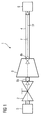
- FIG. 1 shows, in a rough schematic simplification, a steam turbine plant 1 to be simulated (referred to below as plant 1 for short).
- the plant 1 comprises a valve 2, a turbine section 3 and a pipeline 4, which are fluidically connected to one another in series and thus form a fluid path FP for a working fluid F, in particular superheated steam.
- the plant 1 further comprises a valve 2 upstream steam generator 5 and a pipe 4 downstream capacitor. 6
- the real system 1 is first divided into functional Plant elements that are to be mapped to a respective model component of the simulation model 7.
- the valve 2, the turbine section 3 and the pipeline 4 each form such a system element.
- the system 1 is further subdivided into a number of reference volumes 8a and 8b, wherein in each case one reference volume 8a or 8b is interposed between two adjacent system elements 2, 3, 4.
- the reference volume 8a is interposed between the valve 2 and the turbine section 3
- the reference volume 8b is interposed between the turbine section 3 and the pipeline 4.
- the fluid path FP is designed to be linear by connecting the system elements 2, 3, 4 linearly
- the fluid path FP is usually branched like a net.
- the reference volumes are to be arranged in particular in the nodes of the fluid path FP, while the selected plant elements each represent a connection between two such nodes.
- Each reference volume 8a, 8b is selected in such a way that, during operation of the system 1 within the reference volume 8a, 8b, a thermodynamic state which is unambiguous within the scope of the desired accuracy is present at all times, characterized in particular by well-determined thermodynamic state variables such as temperature, pressure, etc. ,
- each reference volume 8a, 8b of Appendix 1 is assigned a memory element 9a or 9b.
- Each memory element 9a, 9b is a software module containing a number of variables and constants is assigned as "Properties”.
- these "properties" comprise a constant virtual volume V whose value is chosen in correspondence with the associated reference volumes 8a and 8b, respectively.
- the state vector Z i comprises as components the pressure p i , the specific volume v i and the specific enthalpy h i of the corresponding memory element 9a or 9b.
- Each plant element 2, 3, 4 is assigned on the part of the simulation model 7 an associated flow function which is specific for the respective plant element 2, 3 or 4 and which is implemented by a corresponding software module, referred to below as flow module 10, 11, 12.
- the flow module 11 outputs the enthalpy h 6 present at the turbine inlet to the upstream storage element 9 a, and the enthalpy h 7 present at the turbine outlet to the downstream storage element 9 b.
- the flow modules 10,11, and 12 are not designed for a fixed flow direction in the rule. Rather, the flow direction is determined flexibly based on the pressure gradient at the module inputs.
- Each memory element 9a, 9b outputs the associated state vector Z 1 , Z 2 as an input state to the adjacent flow modules 10 and 11 or 11 and 12.
- the flow module 11 thus receives, for example, the state vector Z 1 of the upstream memory element 9a and the state vector Z 2 of the downstream memory element 9b as input states.
- a control variable A (in the dimension of one surface) is supplied to the first flow module 10 by a control module 15, through which a variable opening degree of the simulated valve 2 is specified.
- the flow module 11 further outputs an output signal corresponding to the turbine power P to an output module 16.
- each memory element 9a, 9b as well as the initial module 13 and end module 14 are given predetermined states Z 1 to Z 4 as initial conditions.
- an updated state Z 1 or Z 2 is then calculated in the manner described in more detail below as the respective output state and made available again to the adjacent flow modules 10, 11 and 12, respectively.
- a subsequent simulation step the procedure described above is repeated by using the previously calculated output states Z 1 , Z 2 again as initial conditions of the further simulation step. This process is repeated iteratively over a predetermined number of simulation steps until the end of the simulation phase.
- the given edge states Z 3 or Z 4 can optionally be kept constant during the entire simulation phase or varied during the course of the successive simulation steps.
- the simulation conditions can continue to be influenced by variation of the control variable A. For reasons of physical consistency, only physically sensible edge states Z 3 and Z 4 are specified. Likewise, a variation of the edge states Z 3 and Z 4 and the control variable A only takes place continuously with the simulation time.
- enthalpy vector h a vector h
- the respective storage element 9a, 9b is supplied with a vector m (hereinafter referred to as mass vector m), which contains the mass flows m i calculated by the adjacent modules 10, 11, 12, respectively.
- mass vector m ⁇ m 1 , m 2 ⁇ applies here;
- m ⁇ m 2 , m 3 ⁇ applies correspondingly.
- each memory element 9a, 9b the net mass change ⁇ m during the current simulation step is first determined by modules 19, 20 and 21 by summing up the components of the mass vector m.
- this is realized by scalar multiplication (module 21) of the mass vector m with a unit vector containing a number of components of value 1 corresponding to the number of components of the mass vector m.
- the unit vector is generated by component-wise application of a signum function (module 19) to the mass vector m and subsequent component-wise absolute value formation (module 20).
- the memory element 9a, 9b for receiving a variable number of mass flows m 1 ie generalized for processing mass vectors with any number of components.
- the net mass change ⁇ m resulting from the module 21 is supplied to an integrator 22 which updates the stored previous mass content M by adding it to the net mass change ⁇ m.
- ⁇ 1 ! + M ⁇ M where the arrow operator "->" stands for a value assignment to the variable M.
- J ⁇ 1,2 ⁇
- J ⁇ 2,3 ⁇ .
- the sum term in GLG 1 corresponds to a simple sum of the individual mass flows m j .
- the net heat ⁇ Q added or removed to the storage element 9a, 9b during the current simulation step is calculated.
- This is added (module 24) with an additional heat flow ⁇ Q ex , by which a heat loss or gain by radiation or the like is taken into account.
- the addition comprises a further term u ⁇ m, by which the influence of the net mass change ⁇ m on the change of the specific internal energy u is taken into account.
- the result is multiplied by the inverted mass content M- 1 (module 26) and supplied to a second integrator 27 which updates the specific internal energy u of the memory element 9a, 9b.
- the algorithm performed by the modules 23 to 27 is described by the formula ( H ⁇ m + ⁇ Q e x - u ⁇ m ) ⁇ M - 1 + u ⁇ u ,
- the change of the absolute internal energy per iteration step results from the sum mh + ⁇ Q ex .
- a proportional module 32 interposed between the delay module 31 and the module 29 is used to convert the product pv into SI units.
- the enthalpy h i calculated by the module 29 and the specific volume v i calculated by the module 28 are fed to a module 33.
- the module 33 determines the pressure p i with reference to a stored water vapor panel W.
- the pressure p i , the specific volume v i and the enthalpy h i are combined to form the state vector Z i of the respective memory element 9a, 9b and output via a data output 34.
- FIG 4 the structure and operation of the pipeline 4 simulating flow module 12 is shown.
- the flow module 12 is supplied via a first data input 40 of the output from the memory element 9b state vector Z 2 .
- the status vector Z 4 output by the end module 14 is fed to the flow module 12 via a second data input 41.
- the state vector Z 2 and Z 4 From the state vector Z 2 and Z 4 , the corresponding pressures p 2 and p 4 are extracted and fed to a module 42, which determines the pressure difference ⁇ p.
- the flow module 12 is designed to simulate a bidirectional flow through the pipe 4, in which - analogous to the real pipe 4 - the flow direction of the working fluid F is always directed in the direction of the pressure gradient.
- FIG. 4 shows the standard case in which the pressure p 2 in the reference volume 8b exceeds the pressure p 4 in the end module 14 and thus the working fluid F flows from the reference volume 8b in the direction of the condenser 6.
- the specific volume v i is supplied to a module 44.
- the enthalpy h i is output via a data output 45.
- the modules 47 to 49 hereby provide a numerically stabilized root function msqrt (x), which is defined in greater detail in TAB 2.
- the result is multiplied by a module 50 with a constant designated as the design mass flow m 0 and the sign of the pressure difference ⁇ p provided by a module 51 for determining the mass flow m 3 .
- the mass flow m 3 is output via a data output 52.
- the flow module 11, the state vectors Z 1 and Z 2 are supplied via data inputs 53 and 54.
- the flow module 11 outputs the mass flow m 2 via a first data output 55.
- the enthalpy h 6 is output via a second data output 56, the value of which, as already explained above, corresponds to the enthalpy h 1 of the state vector Z 1 .
- Via a third data output 57 the flow module 11 outputs the turbine power P.
- Via a fourth data output 58 the enthalpy h 7 calculated by the flow module 11 is output.
- H 7 H 1 - 100 ⁇ p 1 ⁇ v 1 ⁇ ⁇ ⁇ [ 1 - ( p 2 p 1 ) ( ⁇ - 1 ) / ⁇ ] ⁇ ⁇ ⁇ - 1
- the isentropic exponent ⁇ of water vapor is calculated by a module 59 using the deposited water vapor plate W as a function of the pressure p 1 and the enthalpy h 1 .
- the isentropic efficiency ⁇ of the turbine entering into GLG 4 is provided by a module 60 as a constant.
- Another constant of the value 100 made available by a module 61 is again used to convert the second difference term into GLG 1 into SI units.
- a design flow ⁇ 2 specific to the flow module 11 and the design states is again provided as a constant.
- the mass flow m 2 is calculated according to GLG 5.
- the flow module 10 shown in FIG. 6 is supplied with the state vector Z 3 via a data input 70. Via a second data input 71, the flow module 10 receives the control variable A.
- the state vector Z 1 is supplied via a third data input 73.
- the flow module 10 outputs the calculated mass flow m 1 via a first data output 73.
- the isentropic exponent ⁇ contained therein is replaced by a module 74 again based on the water vapor panel W in Dependence of the pressure p 3 and the enthalpy h 3 determined.
- a design flow rate ⁇ 3 specific to the flow module 10 and the design states is provided as a constant provided by a module 75.
Landscapes
- Engineering & Computer Science (AREA)
- Chemical & Material Sciences (AREA)
- Combustion & Propulsion (AREA)
- Mechanical Engineering (AREA)
- General Engineering & Computer Science (AREA)
- Physics & Mathematics (AREA)
- General Physics & Mathematics (AREA)
- Automation & Control Theory (AREA)
- Control Of Turbines (AREA)
Abstract
Description
- Die Erfindung bezieht sich auf ein Verfahren zur Simulation des Betriebsverhaltens einer Dampfturbinenanlage.
- Ein derartiges Simulationsverfahren wird häufig im Zuge der Konzeption einer Dampfturbinenanlage herangezogen, um bereits vor der Konstruktion der realen, physikalischen Anlagenbestandteile das Betriebsverhalten der zu konstruierenden Anlage abschätzen zu können. Die Simulation dient hierbei insbesondere für eine verbesserte Auslegung bzw. Optimierung der Anlage oder einzelner Anlagebestandteile, zur Früherkennung etwaiger Konzeptionsfehler, etc.
- Ein derartiges Simulationsverfahren wird des Weiteren eingesetzt, um gefahrlos das Betriebsverhalten einer Dampfturbinenanlage in einem außergewöhnlichen Betriebszustand, insbesondere beim schnellen Anfahren der Anlage oder bei Störfällen, zu testen.
- Bisher wird die dynamische Simulation einer Dampfturbinenanlage meistens durch Abbildung der zu simulierenden Anlage auf eine Anzahl von hydrodynamischen Speicher-Drossel-Elementen durchgeführt. Eine hinreichend präzise Modellierung des Massenstroms und des Druckverlaufs innerhalb der Anlage ist bei Anwendung eines solchen Modells in der Regel jedoch nur in der Nähe des untersuchten Arbeitspunktes möglich. Dagegen wird die reale Anlage um so unpräziser abgebildet, je weiter der Betriebszustand von dem untersuchten Arbeitspunkt entfernt ist. Der Temperaturverlauf innerhalb der Anlage lässt sich mit diesem Ansatz nicht nachbilden, ebenso wenig das Verhalten der Anlage bei einem Phasenübergang des Arbeitsfluids.
- Der Erfindung liegt die Aufgabe zu Grunde, ein unter den vorstehend genannten Aspekten verbessertes Verfahren zur Simulation des Betriebsverhaltens einer Dampfturbinenanlage anzugeben.
- Diese Aufgabe wird erfindungsgemäß gelöst durch die Merkmale des Anspruchs 1. Danach wird eine reale (bereits bestehende oder geplante) Dampfturbinenanlage, nachfolgend kurz als Anlage bezeichnet, zunächst durch ein Simulationsmodell abgebildet. Hierzu wird die Anlage in eine Anzahl von Anlagenelemente gegliedert, die jeweils eine funktionale Einheit entlang eines Fluidpfades der Anlage darstellen. Insbesondere wird jede Rohrleitung, jedes Ventil und jeder Turbinenabschnitt der zu simulierenden Anlage als separates Anlagenelement definiert. Weiterhin werden der Anlage ein oder mehrere Referenzvolumina zugeordnet, so dass zwei aneinander angrenzenden Anlagenelementen mindestens ein Referenzvolumen zwischengeordnet ist.
- Jedem Referenzvolumen der realen Dampfturbinenanlage wird nun ein Speicherelement des Simulationsmodells zugeordnet, für das zu jedem Simulationszeitpunkt ein Masseninhalt, ein Energieinhalt sowie ein definierter thermodynamischer Zustand berechnet werden kann. Ebenso wird jedem Anlagenelement der realen Dampfturbinenanlage seitens des Simulationsmodells eine für das Anlagenelement spezifische Durchflussfunktion zugeordnet, die in Abhängigkeit (thermodynamischer) Eingangszustände einen Massenstrom und Enthalpiewerte an den Rändern des Anlagenelements, insbesondere eine ggf. durch das Anlagenelement verursachte Enthalpieänderung berechnet.
- Der (thermodynamische) Zustand eines Speicherelements wird dabei definiert durch ein vorgegebenes Set thermodynamischer Größen, z.B. Druck, Temperatur, Dichte, etc. Der Zustand definiert zeitabhängig den Wert dieser Größen für das zugeordnete Speicherelement.
- Im Zuge einer Simulationsphase ist nun verfahrensgemäß vorgesehen, für jedes Speicherelement ausgehend von vorgegebenen Anfangsbedingungen anhand der Durchflussfunktionen insbesondere iterativ die Masse und den Energieinhalt eines jeden Speicherelements zu berechnen und hieraus einen dem Speicherelement zugeordneten Ausgabezustand abzuleiten.
- Die einem Speicherelement zugeordnete absolute innere Energie ist gemäß der physikalischen Definition dieses Begriffs als Summe der thermischen Energie der in dem Speicherelement enthaltenen Masse gegeben. Anstelle des Absolutbetrages der inneren Energie kann äquivalenterweise die spezifische innere Energie, d.h. die innere Energie pro Masseneinheit, ferner ggf. auch die innere Energie pro Mol, etc., herangezogen werden.
- Als definierende Größen für den Zustand eines Speicherelements sind insbesondere die Größen Druck, Enthalpie und spezifisches Volumen vorgesehen. Als äquivalent zu der Angabe des spezifischen Volumens wird die Angabe der Dichte verstanden, die sich aus dem Kehrwert des spezifischen Volumens ergibt. Es sei hierbei angemerkt, dass an sich durch ein vorgegebenes Wertepaar für zwei dieser Größen ein thermodynamischer Zustand im strengen physikalischen Sinn bereits eindeutig definiert ist, dass also der Wert der jeweils dritten Größe durch ein solches Wertepaar festgelegt ist. Die anmeldungsgemäß redundante Definition eines thermodynamischen Zustands durch Druck, Enthalpie und spezifisches Volumen erfolgt insbesondere zur Reduzierung des mit der Simulation verbundenen Rechenaufwands. Indem der Druck stets wiederum in Abhängigkeit von Enthalpie und spezifischem Volumen bestimmt wird, wird sichergestellt, dass nur physikalisch sinnvolle Zustände berücksichtigt werden.
- Zur Berechnung des einem thermodynamischen Zustand zugeordneten Drucks sowie gegebenenfalls weiterer thermodynamischer Zustandsgrößen wird bevorzugt eine Wasserdampftafel, insbesondere nach dem Industriestandard IAPWS-IF97, herangezogen. Der Begriff Wasserdampftafel bezeichnet ein Kennlinienwerk, in welchem für Wasserdampf die gegenseitige Abhängigkeit thermodynamischer Zustandsgrößen, insbesondere Druck p, Temperatur T, spezifisches Volumen v (bzw. Dichte ρ), Isentropenexponent κ und Enthalpie h, für eine Vielzahl von Zuständen aufgelistet ist. Die Verwendung der Wasserdampftafel im Zuge des Simulationsverfahrens hat insbesondere den Vorteil, dass bei Kenntnis der verfahrensgemäß berechneten inneren Energie und des Masseninhalts eines Speicherelements alle weiteren Zustandsgrößen wie z.B. Druck, Temperatur, Isentropenexponent, etc. einfach abgeleitet werden können.
- Um insbesondere auch komplexere Betriebsabläufe realitätsnah simulieren zu können, umfasst die Simulationsphase bevorzugt mehrere iterativ nacheinander ausgeführte Simulationsschritte, wobei im Zuge eines jeden Simulationsschrittes für jedes Speicherelement ein Ausgabezustand berechnet wird, der wiederum als Anfangsbedingung eines nachfolgend ausgeführten Iterationsschrittes herangezogen wird.
- Weitere Ausbildungen und Vorteile der Erfindung ergeben sich aus dem nachfolgenden Beschreibungsteil, in welchem ein Ausführungsbeispiel der Erfindung anhand einer Zeichnung näher erläutert ist. Darin zeigen:
- FIG 1
- in schematischer Darstellung eine zu simulierende Dampfturbinenanlage mit einem Ventil, einem Turbinenabschnitt und einer Rohrleitung als hintereinander geschaltete Anlagenelemente sowie zwei den Anlagenelementen jeweils zwischengeschalteten Referenzvolumina,
- FIG 2
- in einem Blockschaltbild ein der Dampfturbinenanlage gemäß FIG 1 entsprechendes Simulationsmodell mit zwei jeweils einem Referenzvolumen entsprechenden Speicherelementen sowie jeweils einer dem Ventil, dem Turbinenabschnitt bzw. der Rohrleitung entsprechenden Durchflussfunktion,
- FIG 3
- in einem Blockschaltbild die Struktur eines Speicherelements gemäß FIG 2,
- FIG 4
- in einem Blockschaltbild die der Rohrleitung gemäß FIG 1 entsprechende dritte Durchflussfunktion gemäß FIG 2,
- FIG 5
- in einem Blockschaltbild die dem Turbinenabschnitt gemäß FIG 1 entsprechende zweite Durchflussfunktion gemäß FIG 2 und
- FIG 6
- in einem Blockschaltbild die dem Ventil gemäß FIG 1 entsprechende erste Durchflussfunktion gemäß FIG 2.
- Einander entsprechende Teile und Größen sind in allen Figuren steht mit den gleichen Bezugszeichen versehen. Nachfolgend verwendete mathematische Funktionen und in den Figuren verwendete Symbole sind in TAB 1 und 2 näher erläutert.
- FIG 1 zeigt in grober schematischer Vereinfachung eine zu simulierende Dampfturbinenanlage 1 (nachfolgend kurz als Anlage 1 bezeichnet). Die Anlage 1 umfasst ein Ventil 2, einen Turbinenabschnitt 3 sowie eine Rohrleitung 4, die in Serie fluidisch miteinander verbunden sind und somit einen Fluidpfad FP für ein Arbeitsfluid F, insbesondere Heißdampf, bilden. Die Anlage 1 umfasst weiterhin einen dem Ventil 2 vorgeschalteten Dampferzeuger 5 sowie einen der Rohrleitung 4 nachgeschalteten Kondensator 6.
- Zur Simulation des Betriebsverhaltens der Anlage 1 wird diese zunächst auf ein in FIG 2 dargestelltes Simulationsmodell 7 abgebildet. Zur Erstellung des Simulationsmodells 7 wird die reale Anlage 1 zunächst gegliedert in funktionale Anlagenelemente, die auf jeweils einen entsprechenden Modellbestandteil des Simulationsmodells 7 abgebildet werden sollen. Im Beispiel gemäß FIG 1 bilden das Ventil 2, der Turbinenabschnitt 3 und die Rohrleitung 4 jeweils ein solches Anlagenelement. Um das Betriebsverhalten der Anlage 1 im Zuge der Simulation ortsaufgelöst bestimmen zu können, wird die Anlage 1 weiterhin in eine Anzahl von Referenzvolumina 8a und 8b gegliedert, wobei jeweils ein Referenzvolumen 8a bzw. 8b zwei aneinander angrenzenden Anlagenelementen 2,3,4 zwischengeordnet ist. So ist das Referenzvolumen 8a dem Ventil 2 und dem Turbinenabschnitt 3, und das Referenzvolumen 8b dem Turbinenabschnitt 3 und der Rohrleitung 4 zwischengeordnet.
- Im Gegensatz zu dem vereinfachten Beispiel gemäß FIG 1, bei welchem der Fluidpfad FP durch Hintereinanderschaltung der Anlagenelemente 2,3,4 linear ausgebildet ist, ist bei einer realen Dampfturbinenanlage der Fluidpfad FP in der Regel netzartig verzweigt. In Abbildung einer solchen komplexen Dampfturbinenanlage auf ein entsprechendes Simulationsmodell sind die Referenzvolumina insbesondere in den Knotenpunkten des Fluidpfades FP anzuordnen, während die ausgewählten Anlagenelemente jeweils eine Verbindung zwischen zwei solchen Knotenpunkten darstellen.
- Jedes Referenzvolumen 8a,8b ist derart ausgewählt, dass im Betrieb der Anlage 1 innerhalb des Referenzvolumens 8a, 8b zu jedem Zeitpunkt ein im Rahmen der angestrebten Genauigkeit eindeutiger thermodynamischer Zustand vorliegt, der insbesondere durch wohlbestimmte thermodynamische Zustandsgrößen wie Temperatur, Druck, etc. charakterisiert ist.
- In Abbildung der Anlage 1 auf das Simulationsmodell 7 wird jedem Referenzvolumen 8a, 8b der Anlage 1 ein Speicherelement 9a bzw. 9b zugeordnet. Jedes Speicherelement 9a, 9b ist ein Softwaremodul, dem eine Anzahl von Variablen und Konstanten als "Eigenschaften" zugeordnet ist. Diese "Eigenschaften" umfassen insbesondere ein konstantes virtuelles Volumen V, dessen Wert in Entsprechung mit dem zugeordneten Referenzvolumen 8a bzw. 8b gewählt ist. Des Weiteren sind jedem Speicherelement 9a,9b ein Masseninhalt M und spezifische innere Energie u (u = U/M) als Variablen zugeordnet. Jedem Speicherelement 9a,9b ist weiterhin ein virtueller thermodynamischer Zustand zugeordnet, der in Form eines Datenvektors Zi = {pi,vi,hi} (nachfolgend als Zustandsvektor Zi bezeichnet) definiert ist. Der Zustandsvektor Zi umfasst als Komponenten den Druck pi, das spezifische Volumen vi und die spezifische Enthalpie hi des entsprechenden Speicherelements 9a bzw. 9b. Der Zählindex i=1,2 bezeichnet hierbei die Zuordnung des Zustands Zi und seiner Komponenten pi,vi und hi zu dem jeweiligen Speicherelement 9a bzw. 9b, wobei mit i=1 bezeichnete Größen dem Speicherelement 9a und mit i=2 bezeichnete Größen dem Speicherelement 9b zugeordnet sind.
- Jedem Anlagenelement 2,3,4 ist seitens des Simulationsmodells 7 eine zugehörige und für das jeweilige Anlagenelement 2,3 bzw. 4 spezifische Durchflussfunktion zugeordnet, die durch ein entsprechendes, nachfolgend als Durchflussmodul 10,11,12 bezeichnetes Softwaremodul implementiert ist. Jedes Durchflussmodul 10,11,12 berechnet in Abhängigkeit der thermodynamischen Zustände an den Moduleingängen einen für das jeweilige Durchflussmodul 10,11,12 charakteristischen Massenstrom mi (i=1, 2 ,3) sowie gegebenenfalls eine durch das simulierte Anlagenelement 2,3,4 verursachte Enthalpieänderung. Wird durch das simulierte Anlagenelement keine nennenswerte Änderung der Totalenthalpie verursacht, wie dies aufgrund der adiabatischen Zustandsänderungen im vorliegenden Beispiel für das Ventil 2 und die Rohrleitung 4 der Fall ist, so gibt das zugeordnete Durchflussmodul 10 bzw. 12 zusammen mit dem berechneten Massenstrom mi (mit i=1 für das Durchflussmodul 10, und i=3 für das Durchflussmodul 12) die dementsprechend konstante Enthalpie hi (mit i=5 für für das Durchflussmodul 10, und i=8 für das Durchflussmodul 12) an das jeweils benachbarte Speicherelement 9a bzw. 9b ab. Im Gegensatz dazu wird durch das Durchflussmodul 11 die durch den Turbinenabschnitt 3 verursachte Enthalpieänderung berücksichtigt. Das Durchflussmodul 11 gibt deshalb neben dem berechneten Massenstrom m2 die am Turbineneingang vorliegende Enthalpie h6 an das vorgeschaltete Speicherelement 9a, und die am Turbinenausgang vorliegende Enthalpie h7 an das nachgeschaltete Speicherelement 9b aus. Die Durchflussmodule 10,11,und 12 sind in der Regel nicht für eine feste Durchflussrichtung ausgelegt. Vielmehr wird die Flussrichtung anhand des Druckgefälles an den Moduleingängen flexibel bestimmt.
- Jedes Speicherelement 9a,9b gibt den zugehörigen Zustandsvektor Z1, Z2 als Eingangszustand an die benachbarten Durchflussmodule 10 und 11 bzw. 11 und 12 ab. Das Durchflussmodul 11 erhält also beispielsweise den Zustandsvektor Z1 des vorgeschalteten Speicherelements 9a und den Zustandsvektor Z2 des nachgeschalteten Speicherelements 9b als Eingangszustände.
- Um für die Simulation definierte Randbedingungen zu schaffen, wird dem ersten Durchflussmodul 10 durch ein Initialmodul 13, das die modellhafte Abbildung des Dampferzeugers 5 darstellt, ein vorgegebener Zustand Z3={p3,v3,h3} als Eingangszustand zugeführt. Entsprechend ist dem letzten Durchflussmodul 12 durch ein Endmodul 14, das den Kondensator 6 abbildet, ein Zustand Z4={p4, v4, h4} zugeführt. Bei der nach FIG 1 von dem Dampferzeuger 5 in Richtung auf den Kondensator 6 gerichteten Strömungsrichtung des Arbeitsfluids F gelten für die Werte der Enthalpien hi die Gleichungen h5 = h3, h6 = h1 und h8 = h2.
- Weiterhin wird dem ersten Durchflussmodul 10 durch ein Steuermodul 15 eine Steuergröße A (in der Dimension einer Fläche) zugeführt, durch welche ein variabler Öffnungsgrad des simulierten Ventils 2 vorgegeben ist. Das Durchflussmodul 11 gibt weiterhin ein der Turbinenleistung P entsprechendes Ausgabesignal an ein Ausgabemodul 16 ab.
- Zu Beginn einer Simulationsphase wird jedem Speicherelement 9a,9b sowie dem Initialmodul 13 und Endmodul 14 vorgegebene Zustände Z1 bis Z4 als Anfangsbedingungen vorgegeben. In einem ersten Simulationsschritt wird nun durch jedes Durchflussmodul 10,11,12 der entsprechende Massenstrom mi und die entsprechende Enthalpie hi (i=5-8) berechnet und dem bzw. den benachbarten Speicherelementen 9a und/oder 9b zugeführt. Für jedes Speicherelement 9a,9b wird hierauf in nachfolgend näher beschriebener Weise ein aktualisierter Zustand Z1 bzw. Z2 als jeweiliger Ausgabezustand berechnet und den benachbarten Durchflussmodulen 10,11 bzw. 12 wiederum zur Verfügung gestellt.
- In einem nachfolgenden Simulationsschritt wird der vorstehend beschriebene Vorgang wiederholt, indem die vorher berechneten Ausgabezustände Z1,Z2 wiederum als Anfangsbedingungen des weiteren Simulationsschritts herangezogen werden. Dieser Prozess wird über eine vorgegebene Anzahl von Simulationsschritten iterativ bis zum Ende der Simulationsphase wiederholt. Die vorgegebenen Randzustände Z3 bzw. Z4 können wahlweise, je nach der beabsichtigten Simulationssituation, während der gesamten Simulationsphase konstant gehalten oder im Verlauf der aufeinander folgenden Simulationsschritte variiert werden. Die Simulationsbedingungen können weiterhin durch Variation der Steuergröße A beeinflusst werden. Aus Gründen der physikalischen Konsistenz werden nur physikalisch sinnvolle Randzustände Z3 und Z4 vorgegeben. Ebenso erfolgt eine Variation der Randzustände Z3 und Z4 sowie der Steuergröße A nur stetig mit der Simulationszeit.
- Die Struktur und Funktionsweise eines jeden der beiden Speicherelemente 9a und 9b ist in FIG 3 in einem Blockschaltbild näher dargestellt. Jedes Speicherelement 9a, 9b weist, wie auch schon aus FIG 2 ersichtlich, zwei Dateneingänge 17 und 18 auf. Über den ersten Dateneingang 17 wird dem Speicherelement 9a, 9b ein Vektor h (nachfolgend als Enthalpievektor h bezeichnet) zugeführt, der als Komponenten die von den benachbarten Durchflussmodulen 10,11 bzw. 12 jeweils ausgegebenen Enthalpien hi (i=5-8) enthält. Für das Speicherelement 9a gilt gemäß FIG 2 somit h={h5, h6}, für das Speicherelement 9b entsprechend h={h7, h8}.
- Über den Dateneingang 18 wird dem jeweiligen Speicherelement 9a, 9b ein Vektor m (nachfolgend als Massenvektor m bezeichnet) zugeführt, der die von den benachbarten Modulen 10,11,12 jeweils berechneten Massenströme mi enthält. Für das Speicherelement 9a gilt hier m={m1, m2}, für das Speicherelement 9b gilt entsprechend m={m2, m3}.
- Innerhalb eines jeden Speicherelements 9a, 9b wird zunächst durch Module 19,20 und 21 die Nettomassenänderung Δm während des aktuellen Simulationsschritts bestimmt, indem die Komponenten des Massenvektors m aufsummiert werden. Technisch ist dies realisiert durch Skalarmultiplikation (Modul 21) des Massenvektors m mit einem Einheitsvektor, der eine der Anzahl der Komponenten des Massenvektors m entsprechende Zahl von Komponenten des Werts 1 enthält. Der Einheitsvektor wird erzeugt durch komponentenweise Anwendung einer Signum-Funktion (Modul 19) auf den Massenvektor m und anschließende komponentenweise Absolutwertbildung (Modul 20). Durch diesen numerischen Trick ist das Speicherelement 9a, 9b zur Aufnahme einer variablen Anzahl von Massenströmen m1, d.h. zur Verarbeitung von Massenvektoren mit beliebiger Komponentenanzahl verallgemeinert.
- Die aus dem Modul 21 resultierende Nettomassenänderung Δm wird einem Integrator 22 zugeführt, der den hinterlegten bisherigen Masseninhalt M durch Addition mit der Nettomassenänderung Δm aktualisiert. Die durch die Module 19 bis 22 durchgeführte Massenanpassung ist somit äquivalent mit der Formel

- Aus dem Enthalpievektor h und dem Massenvektor m wird andererseits durch Skalarmultiplikation (Modul 23) die dem Speicherelement 9a,9b während des aktuellen Simulationsschrittes zu- bzw. abgeführte Nettowärme ΔQ berechnet. Diese wird addiert (Modul 24) mit einem zusätzlichen Wärmestrom ΔQex, durch welchen ein Wärmeverlust oder -gewinn durch Abstrahlung oder dgl. berücksichtigt wird. Die Addition umfasst einen weiteren Term uΔm, durch welchen der Einfluss der Nettomassenänderung Δm auf die Änderung der spezifischen inneren Energie u berücksichtigt wird. Das Ergebnis wird mit dem invertierten Masseninhalt M-1 multipliziert (Modul 26) und einem zweiten Integrator 27 zugeführt, der die spezifische innere Energie u des Speicherelements 9a,9b aktualisiert. Der durch die Module 23 bis 27 durchgeführte Algorithmus wird beschrieben durch die Formel

- Aus dem Masseninhalt M wird durch Invertierung (Modul 25) und Multiplikation (Modul 28) mit dem Volumen V das spezifische Volumen vi (i=1,2) berechnet. Anstelle der spezifischen inneren Energie u kann alternativ durch die Speichereinheit 9a, 9b in einer nicht näher dargestellten Verfahrensvariante auch die absolute innere Energie U = M · u direkt berechnet werden. Die Änderung der absoluten inneren Energie pro Iterationsschritt ergibt sich aus der Summe m · h + ΔQex.
- Aus der inneren Energie u wird nach der Formel hi=u+pivi durch ein Modul 29 die spezifische Enthalpie hi des jeweiligen Speicherelements 9a,9b berechnet. Das durch ein Modul 30 gebildete Produkt pv aus Druck pi (i=1,2) und spezifischem Volumen vi wird hierzu durch ein der Auflösung einer algebraischen Schleife dienendes Verzögerungsmodul 31 aus dem vorangegangenem Simulationsschritt zurückbehalten und dem Modul 29 zur Verfügung gestellt. Ein dem Verzögerungsmodul 31 und dem Modul 29 zwischengeschaltetes Proportionalmodul 32 dient zur Umrechnung des Produkts pv in SI-Einheiten. Zur Berechnung des Drucks pi wird die durch das Modul 29 berechnete Enthalpie hi und das durch das Modul 28 berechnete spezifische Volumen vi einem Modul 33 zugeführt. Das Modul 33 ermittelt den Druck pi unter Rückgriff auf eine hinterlegte Wasserdampftafel W.
- Der Druck pi, das spezifische Volumen vi und die Enthalpie hi werden zu dem Zustandsvektor Zi des jeweiligen Speicherelements 9a,9b zusammengefasst und über einen Datenausgang 34 ausgegeben.
- In FIG 4 ist die Struktur und Funktionsweise des die Rohrleitung 4 simulierenden Durchflussmoduls 12 dargestellt. Dem Durchflussmodul 12 wird über einen ersten Dateneingang 40 der von dem Speicherelement 9b ausgegebenen Zustandsvektor Z2 zugeführt. Über einen zweiten Dateneingang 41 wird dem Durchflussmodul 12 der von dem Endmodul 14 ausgegebene Zustandsvektor Z4 zugeführt. Aus dem Zustandsvektor Z2 und Z4 werden die entsprechenden Drücke p2 bzw. p4 extrahiert und einem Modul 42 zugeführt, welches die Druckdifferenz Δp ermittelt. Die Zustandsvektoren Z2 und Z4 werden weiterhin einem Schaltmodul 43 zugeführt, welches entsprechend dem Vorzeichen der Druckdifferenz Δp alternativ den mit dem höheren Druck pi behafteten Zustand Zi (i=2,4) zuschaltet.
- Infolge des Schaltmoduls 43 ist das Durchflussmodul 12 zur Simulation einer bidirektionalen Strömung durch die Rohrleitung 4 ausgebildet, bei welchem - analog zu der realen Rohrleitung 4 - die Strömungsrichtung des Arbeitsfluids F stets in Richtung der Druckgefälles gerichtet ist. In FIG 4 ist der Regelfall dargestellt, in welchem der Druck p2 in dem Referenzvolumen 8b den Druck p4 in dem Endmodul 14 übersteigt und somit das Arbeitsfluid F von dem Referenzvolumen 8b in Richtung des Kondensators 6 strömt.
- Der von dem Schaltmodul 43 ausgegebene Zustandsvektor Zi (gemäß FIG 4: i=2) wird komponentenweise aufgegliedert. Hierbei wird das spezifische Volumen vi einem Modul 44 zugeführt. Die Enthalpie hi wird über einen Datenausgang 45 ausgegeben.
- Durch das Modul 44 wird die Druckdifferenz Δp durch das spezifische Volumen vi und eine als Auslegungsdurchfluss Ψ1 bezeichnete, für das Durchflussmodul 12 spezifische Konstante dividiert. Ψ1 ist hierbei abhängig von dem Auslegungszustand. Von dem Ergebnis wird der Absolutwert (Modul 46) und die Quadratwurzel (Module 47,48 und 49) gebildet. Die Module 47 bis 49 stellen hierbei eine numerisch stabilisierte Wurzelfunktion msqrt(x) zur Verfügung, die in TAB 2 näher definiert ist.
- Das Ergebnis wird durch ein Modul 50 mit einer als Auslegungsmassenstrom m0 bezeichneten Konstante und dem von einem Modul 51 zur Verfügung gestellten Vorzeichen der Druckdifferenz Δp zur Ermittlung des Massenstroms m3 multipliziert. Der Massenstrom m3 wird über einen Datenausgang 52 ausgegeben.
- Der durch die Durchflussgleichung 12 ausgeführte Algorithmus ist somit äquivalent zur der Formel

- In analoger Weise sind in den FIG 5 und 6 die Struktur und Funktionsweise der Durchflussmodule 11 bzw. 10 dargestellt, die den Fluss durch den Turbinenabschnitt 3 bzw. den Fluss durch das Ventil 2 simulieren.
- Dem Durchflussmodul 11 sind über Dateneingänge 53 und 54 die Zustandsvektoren Z1 bzw. Z2 zugeführt. Das Durchflussmodul 11 gibt über einen ersten Datenausgang 55 den Massenstrom m2 aus. Über einen zweiten Datenausgang 56 wird die Enthalpie h6 ausgegeben, deren Wert - wie vorstehend bereits ausgeführt - der Enthalpie h1 des Zustandsvektors Z1 entspricht. Über einen dritten Datenausgang 57 gibt das Durchflussmodul 11 die Turbinenleistung P aus. Über einen vierten Datenausgang 58 wird die von dem Durchflussmodul 11 berechnete Enthalpie h7 ausgegeben. Die Berechnung der Enthalpie h7 folgt hierbei nach der in FIG 5 symbolisch dargestellten Formel

- Hierbei wird der Isentropenexponent κ von Wasserdampf durch ein Modul 59 unter Heranziehung der hinterlegten Wasserdampftafel W in Abhängigkeit des Drucks p1 und der Enthalpie h1 berechnet. Der in GLG 4 eingehende isentrope Wirkungsgrad η der Turbine wird durch ein Modul 60 als Konstante zur Verfügung gestellt. Eine weitere, durch ein Modul 61 zur Verfügung gestellte Konstante des Werts 100 dient wiederum zur Umrechnung des zweiten Differenzterms in GLG 1 in SI-Einheiten.
- Die Berechnung des Massenstroms m2 erfolgt nach der in FIG 5 symbolisch dargestellten Formel

- Durch ein Modul 62 wird hierbei wiederum ein für das Durchflussmodul 11 und die Auslegungszustände spezifischer Auslegungsdurchfluss ψ2 als Konstante zur Verfügung gestellt.
- Die Berechnung der Turbinenleistung P erfolgt nach der in FIG 5 symbolisch dargestellten Formel

- Der Massenstrom m2 berechnet sich hierbei gemäß GLG 5.
- Dem in FIG 6 dargestellten Durchflussmodul 10 wird über einen Dateneingang 70 der Zustandsvektor Z3 zugeführt. Über einen zweiten Dateneingang 71 erhält das Durchflussmodul 10 die Steuergröße A. Über einen dritten Dateneingang 73 ist der Zustandsvektor Z1 zugeführt.
- Das Durchflussmodul 10 gibt den berechneten Massenstrom m1 über einen ersten Datenausgang 73 aus. Die Berechnung des Massenstromes m1 erfolgt hierbei nach der in FIG 6 symbolisch dargestellten Formel


- Die hierin enthaltene Isentropenexponent κ wird durch ein Modul 74 wiederum anhand der Wasserdampftafel W in Abhängigkeit des Drucks p3 und der Enthalpie h3 ermittelt. In GLG 7 geht wiederum ein für das Durchflussmodul 10 und den Auslegungszustände spezifischer Auslegungsdurchfluss ψ3 als Konstante ein, der durch ein Modul 75 bereitgestellt wird.


Claims (7)
- Verfahren zur Simulation des Betriebsverhaltens einer Dampfturbinenanlage (1),- bei welchem die Dampfturbinenanlage (1) in mindestens zwei Anlagenelemente (2,3,4) und mindestens ein Referenzvolumen (8a,8b) gegliedert wird, so dass zwei aneinander angrenzenden Anlagenelementen (2,3;3,4) mindestens ein Referenzvolumen (8a;8b) zwischengeschaltet ist,- bei welchem jedem Referenzvolumen (8a,8b) ein Speicherelement (9a,9b) für Masse und Energie zugeordnet wird, das einen anhand eines vorgegebenen Sets thermodynamischer Größen (pi, vi, hi; i=1,2) definierten zeitabhängigen thermodynamischen Zustand (Zi; i=1, 2) aufweist,- bei welchem dem oder jedem Anlagenelement (2,3,4) eine Durchflussfunktion (10,11,12) zur Ermittlung eines Massenstroms (mi;i=1-3) und zur Ermittlung der Enthalpie (hi ; i=5-8) am Ein- und Austritt des Anlagenelements (2,3,4) zugeordnet wird,wobei im Zuge einer Simulationsphase für jedes Speicherelement (9a, 9b) ausgehend von vorgegebenen Anfangsbedingungen anhand der Durchflussfunktionen (10,11,12) der Masseninhalt (M) und die innere Energie (u) ermittelt und hieraus ein Ausgabezustand berechnet wird.
- Verfahren nach Anspruch 1,
gekennzeichnet durch eine Rohrleitung (4) als Anlagenelement. - Verfahren nach Anspruch 1 oder 2,
gekennzeichnet durch ein Ventil (2) als Anlagenelement. - Verfahren nach einem der Ansprüche 1 bis 3, gekennzeichnet durch einen Turbinenabschnitt (3) als Anlagenelement.
- Verfahren nach einem der Ansprüche 1 bis 4,
dadurch gekennzeichnet, dass der thermodynamische Zustand (Zi; i=1, 2) eines jeden Speicherelements (9a,9b) durch die Größen Druck (pi), Enthalpie (hi) und spezifisches Volumen (vi) definiert wird. - Verfahren nach einem der Ansprüche 1 bis 5,
dadurch gekennzeichnet, dass der Ausgabezustand eines jeden Speicherelements (9a, 9b) unter Heranziehung einer Wasserdampftafel (W) berechnet wird. - Verfahren nach einem der Ansprüche 1 bis 6,
dadurch gekennzeichnet, dass die Simulationsphase mehrere iterativ nacheinander ausgeführte Simulationsschritte umfasst, wobei die für die Speicherelemente (9a,9b) berechneten Ausgabezustände eines zeitlich vorangehenden Simulationsschrittes als Anfangsbedingungen eines zeitlich nachfolgenden Simulationsschrittes herangezogen werden.
Priority Applications (2)
| Application Number | Priority Date | Filing Date | Title |
|---|---|---|---|
| EP04024323A EP1647676B1 (de) | 2004-10-12 | 2004-10-12 | Verfahren zur Simulation des Betriebsverhaltens einer Dampfturbinenanlage |
| EP20050022172 EP1647677B1 (de) | 2004-10-12 | 2005-10-11 | Verfahren zur Simulation des Betriebsverhaltens einer Dampfturbinenanlage |
Applications Claiming Priority (1)
| Application Number | Priority Date | Filing Date | Title |
|---|---|---|---|
| EP04024323A EP1647676B1 (de) | 2004-10-12 | 2004-10-12 | Verfahren zur Simulation des Betriebsverhaltens einer Dampfturbinenanlage |
Publications (2)
| Publication Number | Publication Date |
|---|---|
| EP1647676A1 true EP1647676A1 (de) | 2006-04-19 |
| EP1647676B1 EP1647676B1 (de) | 2013-03-27 |
Family
ID=34926968
Family Applications (1)
| Application Number | Title | Priority Date | Filing Date |
|---|---|---|---|
| EP04024323A Expired - Lifetime EP1647676B1 (de) | 2004-10-12 | 2004-10-12 | Verfahren zur Simulation des Betriebsverhaltens einer Dampfturbinenanlage |
Country Status (1)
| Country | Link |
|---|---|
| EP (1) | EP1647676B1 (de) |
Cited By (2)
| Publication number | Priority date | Publication date | Assignee | Title |
|---|---|---|---|---|
| CN102063066A (zh) * | 2011-01-26 | 2011-05-18 | 田鹤年 | 热电联供式汽轮机数字调节设计运行仿真系统 |
| CN115964854A (zh) * | 2022-11-21 | 2023-04-14 | 兰州空间技术物理研究所 | 一种航天电推进贮供系统仿真建模方法 |
Citations (5)
| Publication number | Priority date | Publication date | Assignee | Title |
|---|---|---|---|---|
| EP0100532A2 (de) * | 1982-08-03 | 1984-02-15 | Siemens Aktiengesellschaft | Verfahren und Einrichtung zur Leistungsregelung an einem Kraftwerksblock |
| US5347466A (en) * | 1991-07-15 | 1994-09-13 | The Board Of Trustees Of The University Of Arkansas | Method and apparatus for power plant simulation and optimization |
| EP0684366A1 (de) * | 1994-05-26 | 1995-11-29 | ABBPATENT GmbH | Verfahren und Einrichtung zur Steuerung und Regelung der Leistung eines Dampfkraftwerksblocks |
| DE19904974A1 (de) * | 1999-02-06 | 2000-08-10 | Abb Patent Gmbh | Verfahren zum Betreiben eines Dampferzeugers unter Einsatz eines Freilastrechners |
| US20040073409A1 (en) * | 1997-01-21 | 2004-04-15 | Siemens Aktiengesellschaft | Method of initializing a simulation of the behavior of an industrial plant, and simulation system for an industrial plant |
-
2004
- 2004-10-12 EP EP04024323A patent/EP1647676B1/de not_active Expired - Lifetime
Patent Citations (5)
| Publication number | Priority date | Publication date | Assignee | Title |
|---|---|---|---|---|
| EP0100532A2 (de) * | 1982-08-03 | 1984-02-15 | Siemens Aktiengesellschaft | Verfahren und Einrichtung zur Leistungsregelung an einem Kraftwerksblock |
| US5347466A (en) * | 1991-07-15 | 1994-09-13 | The Board Of Trustees Of The University Of Arkansas | Method and apparatus for power plant simulation and optimization |
| EP0684366A1 (de) * | 1994-05-26 | 1995-11-29 | ABBPATENT GmbH | Verfahren und Einrichtung zur Steuerung und Regelung der Leistung eines Dampfkraftwerksblocks |
| US20040073409A1 (en) * | 1997-01-21 | 2004-04-15 | Siemens Aktiengesellschaft | Method of initializing a simulation of the behavior of an industrial plant, and simulation system for an industrial plant |
| DE19904974A1 (de) * | 1999-02-06 | 2000-08-10 | Abb Patent Gmbh | Verfahren zum Betreiben eines Dampferzeugers unter Einsatz eines Freilastrechners |
Non-Patent Citations (2)
| Title |
|---|
| NIU Z ET AL: "Adaptive simulation of boiler unit performance", ENERGY CONVERSION AND MANAGEMENT, ELSEVIER SCIENCE PUBLISHERS, OXFORD, GB, vol. 39, no. 13, 1 September 1998 (1998-09-01), pages 1383 - 1394, XP004123264, ISSN: 0196-8904 * |
| SCHAEFER J ET AL: "MATHEMATISCHE MODELLIERUNG EINES DAMPFERZEUGERS MIT ZIRKULIERENDER WIRBELSCHICHT UNTER DER ZIELSETZUNG EINER ECHTZEITSIMULATION", VGB KRAFTWERKSTECHNIK, VGB KRAFTWERKSTECHNIK GMBH. ESSEN, DE, vol. 79, no. 8, 1999, pages 48 - 53, XP000847463, ISSN: 0372-5715 * |
Cited By (3)
| Publication number | Priority date | Publication date | Assignee | Title |
|---|---|---|---|---|
| CN102063066A (zh) * | 2011-01-26 | 2011-05-18 | 田鹤年 | 热电联供式汽轮机数字调节设计运行仿真系统 |
| CN102063066B (zh) * | 2011-01-26 | 2012-05-09 | 田鹤年 | 热电联供式汽轮机数字调节设计运行仿真系统 |
| CN115964854A (zh) * | 2022-11-21 | 2023-04-14 | 兰州空间技术物理研究所 | 一种航天电推进贮供系统仿真建模方法 |
Also Published As
| Publication number | Publication date |
|---|---|
| EP1647676B1 (de) | 2013-03-27 |
Similar Documents
| Publication | Publication Date | Title |
|---|---|---|
| DE69706563T2 (de) | Verfahren zur schaufeltemperaturschätzung in einer dampfturbine | |
| DE4301130C2 (de) | Verfahren und Vorrichtung zum Regeln eines Objektes unter Verwendung einer Lernfunktion | |
| DE102013101025A1 (de) | Verbessertes sequenzielles Verfahren zum Auflösen von Druck-/Durchfluss-Netzwerkparametern in einem verteilten Industrieprozess-Echtzeitsimulationssystem | |
| DE102008038347A1 (de) | Verfahren zur Analyse der Leistungscharakteristik einer Gasturbine und System zur Analyse der Leistungscharakteristik einer Gasturbine | |
| DE102019128655B4 (de) | Verfahren zur Bereitstellung einer rechnergestützten Steuerung für ein technisches System | |
| EP1626317A2 (de) | Verfahren zur Erstellung eines nichtlinearen, stationären oder dynamischen Modells einer Steuergrösse einer Arbeitsmaschine | |
| DE102010025916B4 (de) | Verfahren und Vorrichtung zur Ermittlung von Modellparametern zur Regelung eines Dampfkraftwerksblocks, Regeleinrichtung für einen Dampferzeuger und Computerprogrammprodukt | |
| EP3267338A1 (de) | Verfahren zur berechnung von kerbspannungen in einer schweissnaht | |
| DE102007006616B3 (de) | Verfahren zur Optimierung eines elektronisch gesteuerten automatisch schaltenden Getriebes für ein Kraftfahrzeug | |
| WO2023110612A1 (de) | Verfahren zum bestimmen eines simulierten istmassenstromes in einem kühlmittelkreislauf | |
| EP2088486B1 (de) | Verfahren zur Vermessung eines nichtlinearen dynamischen realen Systems mittels Versuchsplanung | |
| DE102013101028B3 (de) | Schnelles und genaues Verfahren zur Berechnung der kalorischen Größen und des isentropen Zustandes von Gasen und Gemischen aus Gasen | |
| EP1647677B1 (de) | Verfahren zur Simulation des Betriebsverhaltens einer Dampfturbinenanlage | |
| EP2280322B1 (de) | Verfahren zur automatisierten Inbetriebnahme und/oder zum automatisierten Betrieb von Reglern eines elektrischen Antriebssystems mit schwingungsfähiger Mechanik sowie zugehörige Vorrichtung | |
| EP1647676B1 (de) | Verfahren zur Simulation des Betriebsverhaltens einer Dampfturbinenanlage | |
| AT524238B1 (de) | Verfahren zur Ermittlung des Ladezustandes eines Phasenwechselspeichers | |
| DE102016124205A1 (de) | Computer-implementiertes Verfahren zur Optimierung eines Herstellungsprozesses | |
| DE102020116218A1 (de) | Verfahren und Vorrichtung zum Betreiben eines technischen Systems | |
| EP1483633B1 (de) | Verfahren zur simulation eines technischen systems und simulator | |
| DE4340340C1 (de) | Verfahren bzw. Einrichtung zur Bestimmung des Frischdampfmassenstromes in der Frischdampfleitung eines Dampfkraftwerks | |
| EP2517129A1 (de) | Verfahren und prozessrechner zur berechnung der zustandsgrössen eines hybriden differential-algebraischen prozessmodells | |
| DE102020118762A1 (de) | Massenstromschätzung in linksdrehenden Kreisprozessen | |
| DE69016578T2 (de) | Benutzung eines Kondensatableiterwählers zur Auswahl eines Kondensatableiters. | |
| DE102016115331A1 (de) | Verfahren und Vorrichtung zur Bestimmung eines Modells eines technischen Systems | |
| EP1483634A1 (de) | Verfahren zur simulation eines technischen systems und simulator |
Legal Events
| Date | Code | Title | Description |
|---|---|---|---|
| PUAI | Public reference made under article 153(3) epc to a published international application that has entered the european phase |
Free format text: ORIGINAL CODE: 0009012 |
|
| AK | Designated contracting states |
Kind code of ref document: A1 Designated state(s): AT BE BG CH CY CZ DE DK EE ES FI FR GB GR HU IE IT LI LU MC NL PL PT RO SE SI SK TR |
|
| AX | Request for extension of the european patent |
Extension state: AL HR LT LV MK |
|
| 17P | Request for examination filed |
Effective date: 20060508 |
|
| AKX | Designation fees paid |
Designated state(s): CH DE GB IT LI |
|
| GRAP | Despatch of communication of intention to grant a patent |
Free format text: ORIGINAL CODE: EPIDOSNIGR1 |
|
| GRAS | Grant fee paid |
Free format text: ORIGINAL CODE: EPIDOSNIGR3 |
|
| GRAA | (expected) grant |
Free format text: ORIGINAL CODE: 0009210 |
|
| RAP1 | Party data changed (applicant data changed or rights of an application transferred) |
Owner name: SIEMENS AKTIENGESELLSCHAFT |
|
| AK | Designated contracting states |
Kind code of ref document: B1 Designated state(s): CH DE GB IT LI |
|
| REG | Reference to a national code |
Ref country code: GB Ref legal event code: FG4D Free format text: NOT ENGLISH |
|
| REG | Reference to a national code |
Ref country code: CH Ref legal event code: EP |
|
| REG | Reference to a national code |
Ref country code: CH Ref legal event code: NV Representative=s name: SIEMENS SCHWEIZ AG, CH |
|
| REG | Reference to a national code |
Ref country code: DE Ref legal event code: R096 Ref document number: 502004014082 Country of ref document: DE Effective date: 20130523 |
|
| PLBE | No opposition filed within time limit |
Free format text: ORIGINAL CODE: 0009261 |
|
| STAA | Information on the status of an ep patent application or granted ep patent |
Free format text: STATUS: NO OPPOSITION FILED WITHIN TIME LIMIT |
|
| 26N | No opposition filed |
Effective date: 20140103 |
|
| REG | Reference to a national code |
Ref country code: DE Ref legal event code: R097 Ref document number: 502004014082 Country of ref document: DE Effective date: 20140103 |
|
| REG | Reference to a national code |
Ref country code: CH Ref legal event code: PCOW Free format text: NEW ADDRESS: WERNER-VON-SIEMENS-STRASSE 1, 80333 MUENCHEN (DE) |
|
| PGFP | Annual fee paid to national office [announced via postgrant information from national office to epo] |
Ref country code: DE Payment date: 20171219 Year of fee payment: 14 |
|
| PGFP | Annual fee paid to national office [announced via postgrant information from national office to epo] |
Ref country code: CH Payment date: 20180103 Year of fee payment: 14 |
|
| PGFP | Annual fee paid to national office [announced via postgrant information from national office to epo] |
Ref country code: GB Payment date: 20181005 Year of fee payment: 15 Ref country code: IT Payment date: 20181029 Year of fee payment: 15 |
|
| REG | Reference to a national code |
Ref country code: DE Ref legal event code: R119 Ref document number: 502004014082 Country of ref document: DE |
|
| REG | Reference to a national code |
Ref country code: CH Ref legal event code: PL |
|
| PG25 | Lapsed in a contracting state [announced via postgrant information from national office to epo] |
Ref country code: DE Free format text: LAPSE BECAUSE OF NON-PAYMENT OF DUE FEES Effective date: 20190501 |
|
| PG25 | Lapsed in a contracting state [announced via postgrant information from national office to epo] |
Ref country code: LI Free format text: LAPSE BECAUSE OF NON-PAYMENT OF DUE FEES Effective date: 20181031 Ref country code: CH Free format text: LAPSE BECAUSE OF NON-PAYMENT OF DUE FEES Effective date: 20181031 |
|
| GBPC | Gb: european patent ceased through non-payment of renewal fee |
Effective date: 20191012 |
|
| PG25 | Lapsed in a contracting state [announced via postgrant information from national office to epo] |
Ref country code: GB Free format text: LAPSE BECAUSE OF NON-PAYMENT OF DUE FEES Effective date: 20191012 Ref country code: IT Free format text: LAPSE BECAUSE OF NON-PAYMENT OF DUE FEES Effective date: 20191012 |