EP2290545A2 - Monitoring with adaptive dynamic classification - Google Patents
Monitoring with adaptive dynamic classification Download PDFInfo
- Publication number
- EP2290545A2 EP2290545A2 EP10173168A EP10173168A EP2290545A2 EP 2290545 A2 EP2290545 A2 EP 2290545A2 EP 10173168 A EP10173168 A EP 10173168A EP 10173168 A EP10173168 A EP 10173168A EP 2290545 A2 EP2290545 A2 EP 2290545A2
- Authority
- EP
- European Patent Office
- Prior art keywords
- network
- monitored device
- information
- time sequence
- set forth
- Prior art date
- Legal status (The legal status is an assumption and is not a legal conclusion. Google has not performed a legal analysis and makes no representation as to the accuracy of the status listed.)
- Withdrawn
Links
Images


Classifications
-
- G—PHYSICS
- G06—COMPUTING OR CALCULATING; COUNTING
- G06F—ELECTRIC DIGITAL DATA PROCESSING
- G06F11/00—Error detection; Error correction; Monitoring
- G06F11/30—Monitoring
- G06F11/34—Recording or statistical evaluation of computer activity, e.g. of down time, of input/output operation ; Recording or statistical evaluation of user activity, e.g. usability assessment
- G06F11/3466—Performance evaluation by tracing or monitoring
- G06F11/3476—Data logging
-
- G—PHYSICS
- G06—COMPUTING OR CALCULATING; COUNTING
- G06F—ELECTRIC DIGITAL DATA PROCESSING
- G06F11/00—Error detection; Error correction; Monitoring
- G06F11/07—Responding to the occurrence of a fault, e.g. fault tolerance
- G06F11/0703—Error or fault processing not based on redundancy, i.e. by taking additional measures to deal with the error or fault not making use of redundancy in operation, in hardware, or in data representation
- G06F11/0751—Error or fault detection not based on redundancy
-
- G—PHYSICS
- G06—COMPUTING OR CALCULATING; COUNTING
- G06F—ELECTRIC DIGITAL DATA PROCESSING
- G06F11/00—Error detection; Error correction; Monitoring
- G06F11/30—Monitoring
- G06F11/32—Monitoring with visual or acoustical indication of the functioning of the machine
- G06F11/324—Display of status information
- G06F11/328—Computer systems status display
-
- G—PHYSICS
- G06—COMPUTING OR CALCULATING; COUNTING
- G06F—ELECTRIC DIGITAL DATA PROCESSING
- G06F11/00—Error detection; Error correction; Monitoring
- G06F11/30—Monitoring
- G06F11/34—Recording or statistical evaluation of computer activity, e.g. of down time, of input/output operation ; Recording or statistical evaluation of user activity, e.g. usability assessment
- G06F11/3466—Performance evaluation by tracing or monitoring
Definitions
- the following relates to the monitoring arts, classification arts, and related arts, and finds particular application in printing network monitoring arts, electronic network monitoring arts, device network monitoring arts, and so forth.
- a network of printers may be monitored, with selected normal or abnormal events logged.
- the monitoring system is typically a computer (for example, a network server or the like) that occasionally polls a monitored device, network, or system in order to acquire information that is recorded in a monitoring log at the computer or at a storage device in operative communication with the computer.
- the monitored device, network, or system may instead generate log information that is pushed to the monitoring system and recorded in the monitoring log.
- the monitoring log stores discrete observations that are time stamped with the acquisition time.
- the content of the observations may include, for example: sensor readings; operational events (for example, number of color print jobs executed in the case of a printing device); operational status (for example, "on” or "standby” in the case of a printing device); or so forth.
- the information of the monitoring log should be assessed at the monitoring system to ascertain whether the monitored device, network, or system is fully operational, or partially operational (for example, a multi-function printing device may be partially operational if the device operates in printing mode but not in optical scanning mode due to a malfunctioning optical scanner), or non-operational.
- a partial malfunction such as a broken optical scanner may be detected directly (for example, by a sensor that indicates the malfunction) or indirectly (for example, based on a sudden cessation of executed optical scanning jobs by the device).
- the monitoring log is assessed and the device, network, or system is adjusted automatically based on the assessment of the monitoring log.
- Process control approaches are not effective if there is no way to automatically adjust the monitored device, network, or system.
- a malfunctioning printing device generally cannot be automatically fixed, but rather a human repair person is dispatched to repair the printing device.
- Process control approaches may also be less effective if decisions to be made based on the monitoring log are not immediately known.
- a decrease in the number of print jobs executed by a printing device may be an indication of a partial malfunction (such as, for example, the printing device producing printouts with extraneous lines, which may be acceptable for draft prints but not for final documents); on the other hand, the decrease in the number of print jobs executed may be due to other factors such as one or more users being out of the office.
- a monitoring method comprises: recording a time sequence of information pertaining to a monitored device, network, or system comprising observations of and actions taken respective to the monitored device, network, or system; maintaining a hidden Markov model (HMM) operating on the time sequence of information and comprising a hidden state of the monitored device, network, or system; classifying a current state of the monitored device, network, or system using a classification value comprising an emission of the HMM that depends on the hidden state and on a selected portion of the time sequence of information; and generating an action recommendation for the current state of the monitored device, network, or system based on the classification value; wherein at least the maintaining and the classifying are performed by a digital processor.
- HMM hidden Markov model
- a monitoring system comprises: a monitoring module configured to maintain a monitoring log recording a time sequence of information pertaining to a monitored device, network, or system comprising observations of and actions taken respective to the monitored device, network, or system; and a classifier module configured to generate an action recommendation classification based on an estimate of the distribution of a current hidden state of the monitored device, network, or system, a current observation of the monitored device, network, or system, and a selected portion of the time sequence of information prior to the current observation of the monitored device, network, or system.
- a storage medium stores instructions executable by a digital processor to perform an assessment process for assessing a time sequence of information pertaining to a monitored device, network, or system comprising observations of the monitored device, network, or system and actions taken respective to the monitored device, network, or system.
- the assessment process comprises: classifying a current state of a monitored device, network, or system based on an estimate of the distribution of a current hidden state of the monitored device, network, or system and a representation of fixed dimensionality of a current observation and a selected portion of the time sequence of information preceding the current observation in the time sequence; and generating an action recommendation based on the classifying.
- FIGURE 1 diagrammatically shows a monitoring system embodied as a computer configured to monitor a printer network.
- FIGURE 2 diagrammatically shows construction of the classifier module of the monitoring system of FIGURE 1 .
- FIGURE 3 diagrammatically shows the classifier training module of FIGURE 1 .
- FIGURE 4 diagrammatically shows the classifier module of FIGURE 1 .
- an illustrative monitoring system embodied by a computer 10 including a display 12 and keyboard 14 and/or mouse and/or other user input device monitors a printing network.
- the printing network includes a plurality of printing devices 16, 18, 20 (one, some, or all of which may be multifunction printing devices with additional capability such as optical scanning, facsimile transmission, or so forth) that are networked with the monitoring system computer 10 by a communication network 22 such as the Internet, a local area network (LAN), a wireless local area network (WLAN), some combination thereof, or so forth.
- LAN local area network
- WLAN wireless local area network
- the illustrative computer 10 can in general be replaced by any suitably configured digital processing device that includes a digital processor (not shown) that can be variously embodied, such as by a single-core processor, a dual-core processor (or more generally by a multiple-core processor), a digital processor and cooperating math coprocessor, a digital controller, graphical processing unit (GPU), or so forth.
- a digital processor not shown
- the illustrated computer 10 is a desktop or laptop computer including user interfacing components 12, 14.
- Other user interfacing devices such as a second monitor, a mouse or trackball, or so forth can also be included.
- the illustrated computer 10 can be replaced by another digital processing device such as a network server having only network interfacing (for example, Internet or local area network (LAN) interfacing), or so forth.
- the computer 10 is configured by suitable programming, firmware, or so forth to embody the illustrative monitoring system which includes a monitoring module 26 that acquires discrete observations respective to the monitored network or devices 16, 18, 20.
- the monitoring module 26 may acquire discrete observations by actively requesting the information (for example, by actively polling the devices 16, 18, 20) or may acquire discrete observations by passively receiving the information pushed to the computer 10 by the devices 16, 18, 20, or by some combination of push and pull acquisition operations.
- the acquired observations are time stamped with the acquisition time and stored in a monitoring log 30 on a digital storage device (not illustrated; may be internal or external respective to the computer 10) such as a hard drive, optical storage medium, electronic storage medium, or so forth.
- the acquired observation for a printer may, by way of example, include one or more of the following: one or more sensor readings pertaining to toner level, temperature, or other diagnostic parameters; an operational status indicator (for example, having a first value indicating "active", a second value indicating "standby", or so forth); one or more diagnostic parameters indicating, for example, the operational state of components such as an optical scanner, a toner cartridge, and so forth); print media tray indicators (for example, having possible values of "loaded” or "empty”); and so forth.
- the monitoring system may monitor any type of device, network, or system.
- some other contemplated monitored devices, networks, or systems include: a power generation facility (for example, a power station or sub-station, or a power grid of power stations, sub-stations, and the like); one or more heating, ventilating, and air conditioning (HVAC) systems and/or components thereof; a network of computers used by office workers; or so forth.
- HVAC heating, ventilating, and air conditioning
- the monitoring system itself may be variously embodied by one or more digital processing devices.
- the monitoring system embodied by the illustrative computer 10 further includes a classifier module 32 which classifies the state of each monitored network or device 16, 18, 20.
- the classifier module 32 updates the classification when the monitoring module 26 logs an additional observation for the network or device.
- the classifier module 32 employs an adaptive dynamic classifier that generates an informative classification such as a binary classification in which a first binary value represents "device satisfactory" and a (different) second binary value represents "device may have a problem".
- the adaptive dynamic classifier module 32 employs a parameterized classifier using parameters suitably trained by a classifier training module 34.
- the classifier training module 34 may employ a set of independent time sequences extracted from the monitoring log 30 as training data sequences for learning the parameters of the parameterized classifier used by the classifier module 32.
- the informative classification is optionally provided to a human service dispatcher via the display 12 or another user interface.
- the display may show a green indicator whenever the device classification is "device satisfactory" and the indicator may switch to a flashing and/or red indicator whenever the device classification is "device may have a problem".
- the human dispatcher will then perform some remote investigation and possibly dispatch a repair person or team of repair persons to the device which is indicated as possibly having a problem.
- an automated dispatcher module 36 embodied by the computer 10 (as diagrammatically illustrated) or by another digital processing device may be employed.
- the human perceptible display of the informative classification (the illustrative described green or red or flashing indicator) is optionally omitted -- rather, the informative classification serves as a data input to the automated dispatcher 36 which takes remedial action for the classification "device may have a problem" such as automatically dispatching a human repair person or team, or running (further) automated diagnostics.
- the informative classification is also optionally logged in the monitoring log 30. This can be used to assess the accuracy of the classifier module 32 by comparing the informative classification with corresponding "ground truth” information such as (in the illustrative example) a record of the actual operational state of the device, which is also optionally stored in the monitoring log 30. It will be appreciated that this "ground truth" information is also suitably used by the classifier training module 34 in training the classifier module 32.
- the training module 34 and the classifier module 32 may be embodied by different digital processing devices.
- the training module 34 may be embodied by a vendor-owned computer located at a product vendor location
- the classifier module 32 may be embodied by an end user-owned computer located at an end user location different from the vendor location.
- the disclosed classifier and classifier training components 32, 34 can also be embodied as a storage medium storing instructions which when executed on the illustrated computer 10 or on another digital processing device or devices perform the disclosed classifier operations.
- the storage medium may be, for example: a hard disk or other magnetic storage medium; an optical disk or other optical storage medium; a random access memory (RAM) chip or set of RAM chips; a read-only memory (ROM) chip or set of ROM chips; a FLASH memory; or so forth.
- the storage medium may be integral with the computer 10 (for example, an internal hard drive or RAM), or may be separate (for example, an external hard drive operatively connected with the computer 10), or may be separate and accessed via a digital data network such as a local area network (LAN) or the Internet (for example, as a redundant array of inexpensive or independent disks (RAID) or other network server storage that is indirectly accessed by the computer 10 via a digital network).
- LAN local area network
- RAID redundant array of inexpensive or independent disks
- classifier and classifier training components 32, 34 are described.
- “optimization”, “minimization”, and similar phraseology are to be broadly construed as one of ordinary skill in the art would understand these terms. For example, these terms are not to be construed as being limited to the absolute global optimum value, absolute global minimum, or so forth.
- minimization of a function may employ an iterative minimization algorithm that terminates at a stopping criterion before an absolute minimum is reached. It is also contemplated for the optimum or minimum value to be a local optimum or local minimum value.
- the classifier module 32 makes action recommendations respective to remedial actions directed to the monitored devices, network, or system 16, 18, 20.
- the action recommendation is selected from a binary group comprising: (i) no action recommended, and (ii) a remedial action comprising at least investigation should be undertaken for the monitored device, network, or system 16, 18, 20. It is assumed that there exists a ground truth, that is, a correct recommendation or reference decision.
- X and Y represent random variables modeling, respectively, the observation (sometimes referred to as an event) and the corresponding correct recommendation or reference decision (the action, which may in some embodiments include the possible action of "no action taken”).
- Variable X exists in a complex structured space which may involve both discrete and continuous components (for example, results of self-diagnosis procedures, counts, sensor readings, delays, or so forth).
- Variable Y has two possible values, denoted herein as "-1" and "+1".
- the generation of an action recommendation can therefore be viewed as a classification problem in which the goal is to find a predictor ⁇ , which is a (deterministic) function from the data space of the observation random variable X into the binary class space of the action random variable Y which minimizes the expected loss.
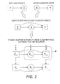
- FIGURE 2 development of the disclosed adaptive dynamic classification approaches operative on time sequences is described starting with simpler static classification approaches operative on static random variables that do not vary in time.
- the topmost and leftmost diagram of FIGURE 2 relates to the na ⁇ ve Bayes approach, which implicitly identifies the class Y with a state of the problem, such that whenever the problem is in a given state, X can be decomposed into independent observations which can be learnt separately.
- the graphical model is shown in FIGURE 2 .
- the distribution of Y is a Bernouilli and that of X
- Y is the independent product of component distributions X ( d )
- Y for d 1: D where D is the dimensionality of the observation space of the observation random variable X .
- Y depends on the nature of component X ( d ) and has an associated parameter in the na ⁇ ve Bayes model.
- a multinomial it is the stochastic vector of probabilities (dimension equal to the cardinality of the range).
- Poisson distribution it is a scalar (the mean of the distribution).
- a Normal or LogNormal distribution it is a pair of scalars (mean and variance).
- Other statistical distributions can also be used in the na ⁇ ve Bayes model approach.
- a state of the problem is advantageous as it corresponds to an abstraction of the state of the monitored system, which is the source of the observed events.
- it is generally insufficient to equate the decision to be made with the state, as in the na ⁇ ve Bayes approach.
- a better approach is to identify the state with some structure capturing rationale leading to the decision, but not the decision itself.
- the distribution of X does not need to be known a priori since it is observed, and the distribution of Y
- X is a Bernouilli distribution whose parameters are determined by a linear combination of the components of X plus the intercept.
- a problem with linear classification approaches is that they do not utilize information about the distribution of X . This is problematic because information about the distribution of X gives information about the possible states of the monitored device, network, or system, and therefore information is effectively lost.
- the na ⁇ ve Bayes and linear classifier approaches are combinable to generate an adaptive mixture of linear classifiers model, as shown in FIGURE 2 .
- This combines the idea of a state on which independent components of the observation stochastically depend, as in na ⁇ ve Bayes approach, and the simple shape of a linear classifier.
- a hidden state variable Z is introduced, which ranges over a finite space of K possible states. The model is shown in FIGURE 2 .
- the distribution of Z is a multinomial, that of X
- X Z is a Bernouilli distribution whose parameters are determined by a linear combination of the components of X plus the intercept, but where the coefficients of the combination depend on Z: there is one vector of coefficients for each possible state of Z.
- the state Z selects the coefficients of the linear classifier.
- Variable Z thus identifies a cluster of observations, and each cluster has its own specific linear classifier for the decision.
- the adaptive mixture of linear classifiers model draws the decision Y from a mixture of linear classifiers whose components are themselves clusters of observations X .
- the na ⁇ ve Bayes, linear classifier, and adaptive mixture of linear classifiers models just described with reference to FIGURE 2 are static models that do not incorporate a time sequence.
- monitoring such as that performed by the monitoring module 26 of FIGURE 1 produces data in the form of time series.
- the action recommendation at a given time might reasonably be expected to be influenced not only by the current state of the device, network, or system, but also by past events (that is, past observations), and even by the past reference decisions, assuming they are known for the past events.
- the possible action recommendations include "do not act” or "perform remedial action including at least investigation”. If the recommendation is to investigate, it is not known at the time this decision is made whether or not it is correct. However, once the investigation is performed it will quickly become manifest whether the investigation was warranted, and hence whether the recommendation to investigate was the correct recommendation. On the other hand, if the recommendation is "do not act”, whether this was the correct recommendation will become manifest shortly thereafter because either nothing bad will happen (in which case the recommendation to not act was correct) or because of some bad effect occurs (in which case the recommendation to not act was not correct).
- the time sequence is indexed by a parameter n where n denotes the current time and n -1, n- 2,... represent prior times.
- n denotes the current time
- n -1, n- 2,... represent prior times.
- X n the current observation
- X n -1 the immediately observation immediately preceding in time
- Y n the current action recommendation to be made (and hence is not known but is to be determined by the model).
- prior (correct) action recommendations Y n -1 , Y n -2 ,... are known.
- X for the static case is replaced by the dynamic dependence Y n
- the known prior (correct) action recommendations Y n -1 , Y n -2 ,... can also be useful information for the inference, so that the inference model is given by Y n
- the inference model can be written as Y n
- an aggregator ⁇ is employed to select a portion of the time sequence of information for use in the inference.
- the final model is depicted at the bottom of FIGURE 2 , where the aggregator ⁇ is diagrammatically represented by a selection box enclosing the selected portion of the time sequence of information that is used in the inference of the current action recommendation Y n .
- the aggregator ⁇ selects the portion of the time sequence of information to be used in the inference and formats it into a representation of fixed dimensionality, such as a vector of a fixed number of components. More generally, the aggregator ⁇ is a deterministic function, optionally controlled by one or more parameters, which takes as input the time sequence of information X n , X n -1 ,..., Y n -1 , Y n -2 ,... of arbitrary length and produces as output a representation of a selected portion of that sequence in a fixed feature space, that is, of a fixed dimensionality.
- the aggregator ⁇ is a sliding window aggregator.
- the aggregated representation of Equation (1) includes a concatenation of: (i) the last r vectors of the time sequence of information (that is, the vectors within the window r ); (ii) for each of the window vectors except the last one, their time distance to the last one; and (iii) a
- the sliding window aggregator can be computed efficiently by induction for all the prefix subsequences of a given sequence, using computationally simple shift and arithmetic operations, and without recomputing each time the two sums in the last component.
- the static term X is replaced by the aggregation of X 1: n , for example using a sliding window aggregator.
- X would now contain r consecutive values of each component of the event vector. To ensure that, conditionally to the state, all these consecutive values are independent would entail an unmanageable number of states, which would characterize not only an abstraction of the state of the monitored system at the time of the observation, but also an abstraction of its most recent evolution.
- the following characterizations of the conditional dependencies of the graphical model of FIGURE 2 are suitable: p ⁇ Z n
- Z n - 1 p ⁇ Z n
- Equation (2) The state dynamics of Equation (2) are controlled by multinomial parameters ⁇ of Markovian dynamics, including a transition matrix and initial vector of dimension, respectively, K ⁇ K and K , with K 2 -1 degrees of freedom.
- the X -emission model of Equation (4) is controlled by a parameter ⁇ kd for each state k and each component d of X.
- Each component d is assumed to be generated according to a member of the same family of distributions, whatever the state k, but the member within that family may depend on k.
- the degree of freedom of parameter ⁇ kd is therefore independent of k but depends on the chosen distribution family for component d .
- the Y -emission model of Equation (5) is controlled by a parameter ⁇ k for each state k , which is the vector of coefficients of the chosen linear classification model.
- the aggregator ⁇ , with corresponding parameter ⁇ can be a sliding window aggregator, but other aggregators are also contemplated.
- the dimension of ⁇ k is that of the image space of ⁇ .
- D ⁇ ( r +1)( D +1): one coefficient for each component of each of X n-r +1: n and the summary of X 1: n-r , one coefficient for each Y n-r +1: n -1 and the summary of Y 1: n-r plus the intercept.
- other information coming from external sources could also be aggregated here.
- such other information could include actual feedback sent to the monitored device, network, or system after each event (if recorded), or the configuration of the device, network, or system (if available), or so forth.
- the dimension D should be modified accordingly.
- FIGURES 3 and 4 Some illustrative embodiments are described with reference to FIGURES 3 and 4 . These illustrative embodiments make the immediate disclosure assumption. For illustrative purposes, these embodiments employ binary logistic regression (LR) as the linear classifier; however, substantially any other probabilistic linear classifier would work as well.
- LR binary logistic regression
- x) ⁇ ( y ⁇ T x) where ⁇ is the vector of coefficients (including intercept) and ⁇ denotes the logistic (sigmoid) function.
- the s time sequences may, for example, correspond to logs of different devices.
- a supervised machine learning module 42 optimizes parameters of a parameterized classifier employing a hidden Markov model (HMM) 46 as set forth herein with reference to Equations (1)-(6) to generate trained classifier parameters 48.
- HMM hidden Markov model
- FIGURE 2 An illustrative example of a suitable supervised machine learning algorithm employing the expectation-maximization (EM) process is described.
- K that is, the number of states
- ⁇ the aggregator parameter
- the model of FIGURE 2 is designed in such a way that the learning of the event component models Z ⁇ X ( d ) on the one hand and that of the linear classifiers Z , X ⁇ ⁇ Y on the other hand, can be done in a modular fashion (although not independently).
- the EM algorithm can be used here, and more precisely its version for HMM called Baum-Welch (see Rabiner, "A tutorial on hidden markov models and selected applications in speech recognition", in Proceedings of the IEEE vo. 77 no. 2, pp.
- the Baum-Welch algorithm entails defining two operations, one in the E-step and one in the M-step, as follows.
- the solution can be inexact. Exploiting the property of generalized EM, it is sufficient to increase the objective with respect to the current parameters rather than actually maximize it. This is particularly relevant if any of the independent fit tasks in the M-step is obtained by an anytime iterative process. In that case, the number of iterations can be bounded arbitrarily, rather than by waiting for the variation in objective to go under a threshold, as is usually done. For standard simple distributions such as multinomials, Poisson, normals, log-normals, and so forth, there exist analytical formulas to estimate the parameters. On the other hand, the estimation of the coefficients of a logistic regression is usually based on a convex optimization algorithm which is iterative.
- the structural parameters ⁇ , K can be chosen empirically or learnt from the data by systematic enumeration. To avoid overfitting, the BIC criterion (see Schwartz, "Estimating the dimension of a model", Annals of Statistics, vol. 6 no. 2 pp.
- ⁇ * ⁇ K * arg min ⁇ K - 2 ⁇ log ⁇ L K ⁇ ⁇ + F K ⁇ log ⁇ N
- L ( K , ⁇ ) is the maximized likelihood of the data in the model with an aggregator controlled by ⁇ and K states
- F ( K ) is its degree of freedom, given by Equation (6)
- N is the number of independent instances (here the number of time series in the training data).
- the classifier module 32 which uses the parameterized classifier employing a hidden Markov model (HMM) 46 with the trained classifier parameters 48 is described.
- the classifier module 32 performs the inference operation: where ⁇ is the trained classifier parameters 48, x 1: n represents the observations logged in the monitoring log 30, y 1: n -1 represents the past (correct) action recommendations (that is, the reference decisions) logged in the monitoring log 30, and n represents the current action recommendation to be generated by the classifier module 32.
- the inference operation of Equation (11) utilizes the HMM 46 comprising the trained classifier 32, 34, the hidden state 50 of the monitored device, network, or system, and the selected portion of the time sequence of information to generate a classification value or prediction y n 52.
- the classification value or prediction y n 52 has a value of either -1 or 1 representing whether or not an action including investigation should be taken.
- a recommendation output generator 54 formats the classification value or prediction y n 52 into a more human-friendly output for display to a human dispatcher or other user; or, alternatively or additionally, the recommendation output generator 54 may format the classification value or prediction y n 52 into a suitable input for the automated dispatcher 36.
- K a coefficient of HMM
- the prediction y n is then obtained by comparing the conditional probability given by Equation (17) to a threshold. If the objective is to maximise the accuracy of the classification, then the threshold is simply set to 0.5. If the precision of the classification for one of the classes is to be favoured, then the threshold can be determined by a ROC curve analysis, where the ROC curve is determined, for example, by cross validation.
Landscapes
- Engineering & Computer Science (AREA)
- Theoretical Computer Science (AREA)
- General Engineering & Computer Science (AREA)
- Quality & Reliability (AREA)
- Physics & Mathematics (AREA)
- General Physics & Mathematics (AREA)
- Computer Hardware Design (AREA)
- Computing Systems (AREA)
- Management, Administration, Business Operations System, And Electronic Commerce (AREA)
- Data Exchanges In Wide-Area Networks (AREA)
- Debugging And Monitoring (AREA)
Abstract
Description
- The following relates to the monitoring arts, classification arts, and related arts, and finds particular application in printing network monitoring arts, electronic network monitoring arts, device network monitoring arts, and so forth.
- Monitoring of networks and systems is a common task. As an illustrative example, a network of printers may be monitored, with selected normal or abnormal events logged. The monitoring system is typically a computer (for example, a network server or the like) that occasionally polls a monitored device, network, or system in order to acquire information that is recorded in a monitoring log at the computer or at a storage device in operative communication with the computer. In addition to or instead of polling, the monitored device, network, or system may instead generate log information that is pushed to the monitoring system and recorded in the monitoring log. In either case, the monitoring log stores discrete observations that are time stamped with the acquisition time. The content of the observations may include, for example: sensor readings; operational events (for example, number of color print jobs executed in the case of a printing device); operational status (for example, "on" or "standby" in the case of a printing device); or so forth.
- To be useful, the information of the monitoring log should be assessed at the monitoring system to ascertain whether the monitored device, network, or system is fully operational, or partially operational (for example, a multi-function printing device may be partially operational if the device operates in printing mode but not in optical scanning mode due to a malfunctioning optical scanner), or non-operational. A partial malfunction such as a broken optical scanner may be detected directly (for example, by a sensor that indicates the malfunction) or indirectly (for example, based on a sudden cessation of executed optical scanning jobs by the device). In a process control approach the monitoring log is assessed and the device, network, or system is adjusted automatically based on the assessment of the monitoring log.
- Process control approaches are not effective if there is no way to automatically adjust the monitored device, network, or system. For example, a malfunctioning printing device generally cannot be automatically fixed, but rather a human repair person is dispatched to repair the printing device. Process control approaches may also be less effective if decisions to be made based on the monitoring log are not immediately known. For example, a decrease in the number of print jobs executed by a printing device may be an indication of a partial malfunction (such as, for example, the printing device producing printouts with extraneous lines, which may be acceptable for draft prints but not for final documents); on the other hand, the decrease in the number of print jobs executed may be due to other factors such as one or more users being out of the office.
- In such cases, it could nonetheless still be advantageous to assess the monitoring log in order to make a decision as to whether action is needed, or whether a particular action should be taken. Such assessment can lead to more efficient deployment of human resources (for example, human repair persons or teams), or more accurate decisions of high consequence (for example, a decision to shut down a power generation plant of an electrical grid), or so forth.
- In some illustrative embodiments disclosed as illustrative examples herein, a monitoring method comprises: recording a time sequence of information pertaining to a monitored device, network, or system comprising observations of and actions taken respective to the monitored device, network, or system; maintaining a hidden Markov model (HMM) operating on the time sequence of information and comprising a hidden state of the monitored device, network, or system; classifying a current state of the monitored device, network, or system using a classification value comprising an emission of the HMM that depends on the hidden state and on a selected portion of the time sequence of information; and generating an action recommendation for the current state of the monitored device, network, or system based on the classification value; wherein at least the maintaining and the classifying are performed by a digital processor.
- In some illustrative embodiments disclosed as illustrative examples herein, a monitoring system comprises: a monitoring module configured to maintain a monitoring log recording a time sequence of information pertaining to a monitored device, network, or system comprising observations of and actions taken respective to the monitored device, network, or system; and a classifier module configured to generate an action recommendation classification based on an estimate of the distribution of a current hidden state of the monitored device, network, or system, a current observation of the monitored device, network, or system, and a selected portion of the time sequence of information prior to the current observation of the monitored device, network, or system.
- In some illustrative embodiments disclosed as illustrative examples herein, a storage medium stores instructions executable by a digital processor to perform an assessment process for assessing a time sequence of information pertaining to a monitored device, network, or system comprising observations of the monitored device, network, or system and actions taken respective to the monitored device, network, or system. The assessment process comprises: classifying a current state of a monitored device, network, or system based on an estimate of the distribution of a current hidden state of the monitored device, network, or system and a representation of fixed dimensionality of a current observation and a selected portion of the time sequence of information preceding the current observation in the time sequence; and generating an action recommendation based on the classifying.
-
FIGURE 1 diagrammatically shows a monitoring system embodied as a computer configured to monitor a printer network. -
FIGURE 2 diagrammatically shows construction of the classifier module of the monitoring system ofFIGURE 1 . -
FIGURE 3 diagrammatically shows the classifier training module ofFIGURE 1 . -
FIGURE 4 diagrammatically shows the classifier module ofFIGURE 1 . - With reference to
FIGURE 1 , an illustrative monitoring system embodied by acomputer 10 including adisplay 12 andkeyboard 14 and/or mouse and/or other user input device monitors a printing network. The printing network includes a plurality ofprinting devices monitoring system computer 10 by acommunication network 22 such as the Internet, a local area network (LAN), a wireless local area network (WLAN), some combination thereof, or so forth. Theillustrative computer 10 can in general be replaced by any suitably configured digital processing device that includes a digital processor (not shown) that can be variously embodied, such as by a single-core processor, a dual-core processor (or more generally by a multiple-core processor), a digital processor and cooperating math coprocessor, a digital controller, graphical processing unit (GPU), or so forth. By way of example, the illustratedcomputer 10 is a desktop or laptop computer includinguser interfacing components computer 10 can be replaced by another digital processing device such as a network server having only network interfacing (for example, Internet or local area network (LAN) interfacing), or so forth. - The
computer 10 is configured by suitable programming, firmware, or so forth to embody the illustrative monitoring system which includes amonitoring module 26 that acquires discrete observations respective to the monitored network ordevices monitoring module 26 may acquire discrete observations by actively requesting the information (for example, by actively polling thedevices computer 10 by thedevices monitoring log 30 on a digital storage device (not illustrated; may be internal or external respective to the computer 10) such as a hard drive, optical storage medium, electronic storage medium, or so forth. In the illustrative embodiment, the acquired observation for a printer may, by way of example, include one or more of the following: one or more sensor readings pertaining to toner level, temperature, or other diagnostic parameters; an operational status indicator (for example, having a first value indicating "active", a second value indicating "standby", or so forth); one or more diagnostic parameters indicating, for example, the operational state of components such as an optical scanner, a toner cartridge, and so forth); print media tray indicators (for example, having possible values of "loaded" or "empty"); and so forth. - It is to be appreciated that the foregoing are merely illustrative examples. In general, the monitoring system may monitor any type of device, network, or system. By way of example, some other contemplated monitored devices, networks, or systems include: a power generation facility (for example, a power station or sub-station, or a power grid of power stations, sub-stations, and the like); one or more heating, ventilating, and air conditioning (HVAC) systems and/or components thereof; a network of computers used by office workers; or so forth. As already noted, the monitoring system itself may be variously embodied by one or more digital processing devices.
- The monitoring system embodied by the
illustrative computer 10 further includes aclassifier module 32 which classifies the state of each monitored network ordevice classifier module 32 updates the classification when themonitoring module 26 logs an additional observation for the network or device. As disclosed herein, theclassifier module 32 employs an adaptive dynamic classifier that generates an informative classification such as a binary classification in which a first binary value represents "device satisfactory" and a (different) second binary value represents "device may have a problem". The adaptivedynamic classifier module 32 employs a parameterized classifier using parameters suitably trained by aclassifier training module 34. For example, as disclosed herein theclassifier training module 34 may employ a set of independent time sequences extracted from themonitoring log 30 as training data sequences for learning the parameters of the parameterized classifier used by theclassifier module 32. - The informative classification is optionally provided to a human service dispatcher via the
display 12 or another user interface. For example, the display may show a green indicator whenever the device classification is "device satisfactory" and the indicator may switch to a flashing and/or red indicator whenever the device classification is "device may have a problem". Typically, it is expected that the human dispatcher will then perform some remote investigation and possibly dispatch a repair person or team of repair persons to the device which is indicated as possibly having a problem. - Alternatively, an
automated dispatcher module 36 embodied by the computer 10 (as diagrammatically illustrated) or by another digital processing device may be employed. In such embodiments, the human perceptible display of the informative classification (the illustrative described green or red or flashing indicator) is optionally omitted -- rather, the informative classification serves as a data input to theautomated dispatcher 36 which takes remedial action for the classification "device may have a problem" such as automatically dispatching a human repair person or team, or running (further) automated diagnostics. - The informative classification is also optionally logged in the
monitoring log 30. This can be used to assess the accuracy of theclassifier module 32 by comparing the informative classification with corresponding "ground truth" information such as (in the illustrative example) a record of the actual operational state of the device, which is also optionally stored in themonitoring log 30. It will be appreciated that this "ground truth" information is also suitably used by theclassifier training module 34 in training theclassifier module 32. - In some variant embodiments, the
training module 34 and theclassifier module 32 may be embodied by different digital processing devices. For example, thetraining module 34 may be embodied by a vendor-owned computer located at a product vendor location, while theclassifier module 32 may be embodied by an end user-owned computer located at an end user location different from the vendor location. It will be further appreciated that the disclosed classifier andclassifier training components computer 10 or on another digital processing device or devices perform the disclosed classifier operations. The storage medium (not shown) may be, for example: a hard disk or other magnetic storage medium; an optical disk or other optical storage medium; a random access memory (RAM) chip or set of RAM chips; a read-only memory (ROM) chip or set of ROM chips; a FLASH memory; or so forth. The storage medium may be integral with the computer 10 (for example, an internal hard drive or RAM), or may be separate (for example, an external hard drive operatively connected with the computer 10), or may be separate and accessed via a digital data network such as a local area network (LAN) or the Internet (for example, as a redundant array of inexpensive or independent disks (RAID) or other network server storage that is indirectly accessed by thecomputer 10 via a digital network). - In the following, some illustrative examples of the classifier and
classifier training components - The
classifier module 32 makes action recommendations respective to remedial actions directed to the monitored devices, network, orsystem system - In the following, X and Y represent random variables modeling, respectively, the observation (sometimes referred to as an event) and the corresponding correct recommendation or reference decision (the action, which may in some embodiments include the possible action of "no action taken"). Variable X exists in a complex structured space which may involve both discrete and continuous components (for example, results of self-diagnosis procedures, counts, sensor readings, delays, or so forth). Variable Y has two possible values, denoted herein as "-1" and "+1". The generation of an action recommendation can therefore be viewed as a classification problem in which the goal is to find a predictor Ŷ, which is a (deterministic) function from the data space of the observation random variable X into the binary class space of the action random variable Y which minimizes the expected loss.
- With reference to
FIGURE 2 , development of the disclosed adaptive dynamic classification approaches operative on time sequences is described starting with simpler static classification approaches operative on static random variables that do not vary in time. The topmost and leftmost diagram ofFIGURE 2 relates to the naïve Bayes approach, which implicitly identifies the class Y with a state of the problem, such that whenever the problem is in a given state, X can be decomposed into independent observations which can be learnt separately. The graphical model is shown inFIGURE 2 . The distribution of Y is a Bernouilli and that of X|Y is the independent product of component distributions X (d)|Y for d = 1:D where D is the dimensionality of the observation space of the observation random variable X . Each distribution X (d)|Y depends on the nature of component X (d) and has an associated parameter in the naïve Bayes model. For a multinomial, it is the stochastic vector of probabilities (dimension equal to the cardinality of the range). For a Poisson distribution, it is a scalar (the mean of the distribution). For a Normal or LogNormal distribution, it is a pair of scalars (mean and variance). Other statistical distributions can also be used in the naïve Bayes model approach. - The idea of a "state" of the problem is advantageous as it corresponds to an abstraction of the state of the monitored system, which is the source of the observed events. On the other hand, it is generally insufficient to equate the decision to be made with the state, as in the naïve Bayes approach. As recognized herein, a better approach is to identify the state with some structure capturing rationale leading to the decision, but not the decision itself.
- With continuing reference to
FIGURE 2 , other approaches comprise the linear classification approaches, which assume that the form of the predictor is defined by a hyperplane in the space of the observation random variable X. If the observations X include discrete components, these can be accommodated by adding a continuous dimension for each possible value of the discrete component. Logistic regression is a typical example of a linear classifier, and its graphical model is shown in the topmost and rightmost diagram ofFIGURE 2 . - In the linear classification approaches, the distribution of X does not need to be known a priori since it is observed, and the distribution of Y|X is a Bernouilli distribution whose parameters are determined by a linear combination of the components of X plus the intercept. A problem with linear classification approaches is that they do not utilize information about the distribution of X. This is problematic because information about the distribution of X gives information about the possible states of the monitored device, network, or system, and therefore information is effectively lost.
- With continuing reference to
FIGURE 2 , the naïve Bayes and linear classifier approaches are combinable to generate an adaptive mixture of linear classifiers model, as shown inFIGURE 2 . This combines the idea of a state on which independent components of the observation stochastically depend, as in naïve Bayes approach, and the simple shape of a linear classifier. Toward this end, a hidden state variable Z is introduced, which ranges over a finite space of K possible states. The model is shown inFIGURE 2 . The distribution of Z is a multinomial, that of X|Z is the product of independent component distributions X (d)|Z as in the naïve Bayes case, and Y|X Z is a Bernouilli distribution whose parameters are determined by a linear combination of the components of X plus the intercept, but where the coefficients of the combination depend on Z: there is one vector of coefficients for each possible state of Z. In effect, the state Z selects the coefficients of the linear classifier. Variable Z thus identifies a cluster of observations, and each cluster has its own specific linear classifier for the decision. Viewed yet another way, the adaptive mixture of linear classifiers model draws the decision Y from a mixture of linear classifiers whose components are themselves clusters of observations X. - The naïve Bayes, linear classifier, and adaptive mixture of linear classifiers models just described with reference to
FIGURE 2 are static models that do not incorporate a time sequence. On the other hand, monitoring such as that performed by themonitoring module 26 ofFIGURE 1 produces data in the form of time series. The action recommendation at a given time might reasonably be expected to be influenced not only by the current state of the device, network, or system, but also by past events (that is, past observations), and even by the past reference decisions, assuming they are known for the past events. - Knowledge of past reference decisions (that is, the "correct" recommendation at a given point in time in the past) is typically known in the case of binary decisions because the observer sees the consequences of its previous decisions and can thereby infer, immediately or shortly after having applied the decision, whether the action recommendation was correct or incorrect. This is referred to herein as the "immediate disclosure" assumption - it is assumed that the correct recommendation (i.e., reference decision) is known for all past events (but obviously not for the current event).
- For example, consider an illustrative case in which the possible action recommendations include "do not act" or "perform remedial action including at least investigation". If the recommendation is to investigate, it is not known at the time this decision is made whether or not it is correct. However, once the investigation is performed it will quickly become manifest whether the investigation was warranted, and hence whether the recommendation to investigate was the correct recommendation. On the other hand, if the recommendation is "do not act", whether this was the correct recommendation will become manifest shortly thereafter because either nothing bad will happen (in which case the recommendation to not act was correct) or because of some bad effect occurs (in which case the recommendation to not act was not correct).
- With continuing reference to
FIGURE 2 , it is desired to extend the adaptive mixture of linear classifiers model to the case of a time sequence. In the following, the time sequence is indexed by a parameter n where n denotes the current time and n-1, n-2,... represent prior times. Thus, the current observation is denoted Xn while the immediately observation immediately preceding in time is denoted X n-1, and so forth. The correct action recommendations are similarly denoted Yn , Y n-1,..., where Yn is the current action recommendation to be made (and hence is not known but is to be determined by the model). Under the immediate disclosure assumption, it is assumed that prior (correct) action recommendations Y n-1, Y n-2,... are known. In this case, the dependence Y|X for the static case is replaced by the dynamic dependence Yn |Xn ,X n-1,.... Moreover, the known prior (correct) action recommendations Y n-1, Y n-2,... can also be useful information for the inference, so that the inference model is given by Yn |Xn ,X n-1 ,...,Y n-1,Y n-2,.... Further allowing for the hidden state variable Z the inference model can be written as Yn |Xn ,X n-1,...,Y n-1,Y n-2,...,Zn where Zn is the current state of the hidden state variable Z. - With continuing reference to
FIGURE 2 , in practice it is not computationally convenient to include all past information Xn ,X n-1,...,Y n-1,Y n-2,... in the inference model, because this information is of variable length and constantly enlarging as the monitoring process proceeds. Accordingly, an aggregator Φ is employed to select a portion of the time sequence of information for use in the inference. The final model is depicted at the bottom ofFIGURE 2 , where the aggregator Φ is diagrammatically represented by a selection box enclosing the selected portion of the time sequence of information that is used in the inference of the current action recommendation Yn . The aggregator Φ selects the portion of the time sequence of information to be used in the inference and formats it into a representation of fixed dimensionality, such as a vector of a fixed number of components. More generally, the aggregator Φ is a deterministic function, optionally controlled by one or more parameters, which takes as input the time sequence of information Xn ,X n-1,...,Y n-1,Y n-2,... of arbitrary length and produces as output a representation of a selected portion of that sequence in a fixed feature space, that is, of a fixed dimensionality. - In some illustrative embodiments, the aggregator Φ is a sliding window aggregator. The sequence to aggregate is suitably represented as


The aggregated representation of Equation (1) includes a concatenation of: (i) the last r vectors of the time sequence of information (that is, the vectors within the window r); (ii) for each of the window vectors except the last one, their time distance to the last one; and (iii) a weighted sum of all remaining vectors, before the window in the time sequence of information, wherein the weights are chosen such that items decay with time, and a represents the rate at which older items lose weight in the sum. Optionally, the decay portion is omitted, and the sliding window aggregator is
- In one approach for extending the adaptive mixture of linear classifiers model to a time sequence of information, the static term X is replaced by the aggregation of X 1:n , for example using a sliding window aggregator. However, in that case, the assumption that in a given state Z, the components of X are independent becomes unreasonable. Indeed, X would now contain r consecutive values of each component of the event vector. To ensure that, conditionally to the state, all these consecutive values are independent would entail an unmanageable number of states, which would characterize not only an abstraction of the state of the monitored system at the time of the observation, but also an abstraction of its most recent evolution.
- As an alternative approach, it is disclosed herein to keep the original observation vector X reduced to the event vector, and transform the graphical model to account for the sequence structure of the events. This is achieved by assuming hidden Markov dynamics for state Z. Furthermore, since X is observed anyway at each instance, it does not cost anything to make Yn depend not only on XnZn as specified by the graphical model, but also on X 1:n-1. With the immediate disclosure assumption, Yn can optionally also be made dependent on Y 1:n-1, still at no cost. In this approach Yn depends on a variable length sequence of observations, which can be aggregated by a sliding window aggregator or another a suitable aggregator. Although this model introduces a dependency of component Y of the emission on potentially all its predecessors, the Markov dynamics of the states Z is still of
order 1. The graphical model becomes that shown inFIGURE 2 ("Dynamic Adaptive Mixture of Linear Classifiers Model, Extended to a Time Sequence"), and is equivalent to the following factorization of the generative model:
The following characterizations of the conditional dependencies of the graphical model ofFIGURE 2 are suitable:

and
- The state dynamics of Equation (2) are controlled by multinomial parameters ρ of Markovian dynamics, including a transition matrix and initial vector of dimension, respectively, K × K and K, with K 2 -1 degrees of freedom.
- The X -emission model of Equation (4) is controlled by a parameter θ kd for each state k and each component d of X. Each component d is assumed to be generated according to a member of the same family of distributions, whatever the state k, but the member within that family may depend on k. The degree of freedom of parameter θ kd is therefore independent of k but depends on the chosen distribution family for component d.
- The Y-emission model of Equation (5) is controlled by a parameter β k for each state k, which is the vector of coefficients of the chosen linear classification model. Thus, in state k, the binary emission Yn follows a Bernouilli distribution whose parameter is determined by the scalar product

- Optionally, other information coming from external sources could also be aggregated here. For example, such other information could include actual feedback sent to the monitored device, network, or system after each event (if recorded), or the configuration of the device, network, or system (if available), or so forth. In such cases, the dimension D should be modified accordingly.
- Given Kµ, the total degree of freedom of the overall parameter is therefore:

- Having set forth a suitable dynamic adaptive classifier for use with a time sequence of information such as the
monitoring log 30 generated by themonitoring module 26, some illustrative embodiments are described with reference toFIGURES 3 and 4 . These illustrative embodiments make the immediate disclosure assumption. For illustrative purposes, these embodiments employ binary logistic regression (LR) as the linear classifier; however, substantially any other probabilistic linear classifier would work as well. In a LR model, if x is the input (with an extra component set to 1) and y the output (in {-1,1}), then p(y|x) = σ(yβ T x) where β is the vector of coefficients (including intercept) and σ denotes the logistic (sigmoid) function. - With reference to
FIGURE 3 , theclassifier training module 34 receives as input atraining sequence 40 comprising a set s = 1,...,N of independent time sequences of information
monitoring log 30. The s time sequences may, for example, correspond to logs of different devices. A supervisedmachine learning module 42 optimizes parameters of a parameterized classifier employing a hidden Markov model (HMM) 46 as set forth herein with reference to Equations (1)-(6) to generate trainedclassifier parameters 48. That is, the supervisedmachine learning module 42 performs the learning process:
where Θ denotes the trainedclassifier parameters 48. - An illustrative example of a suitable supervised machine learning algorithm employing the expectation-maximization (EM) process is described. First consider the case where the structural parameters K (that is, the number of states) and µ (the aggregator parameter) are set. The model of
FIGURE 2 is designed in such a way that the learning of the event component models Z → X (d) on the one hand and that of the linear classifiers Z, X̃ → Y on the other hand, can be done in a modular fashion (although not independently). The EM algorithm can be used here, and more precisely its version for HMM called Baum-Welch (see Rabiner, "A tutorial on hidden markov models and selected applications in speech recognition", in Proceedings of the IEEE vo. 77 no. 2, pp. 257-86 (1989)), with Z as state variable and XY as emission. For parameter ρ characterizing the discrete state dynamic, no constraint is imposed on the parameter, meaning that any state can a priori be reached from any other state or itself. On the side of the emission parameters, the Baum-Welch algorithm entails defining two operations, one in the E-step and one in the M-step, as follows. - In the E-step, given a sequence of points in the emission space (i.e. that of XY ), compute for each point and each possible value k of Z the probability (or density) at the end point, given Z = k at that point and given the current values of the parameters β k θ k(1:D). By combining Equations (4) and (5), an expression is obtained of P((XY)n |Zn(XY) 1:n-1).
- In the M-step, given an empirical distribution in the emission space for each possible value k of Z , compute the parameters β k θ k(1:D) which best fit that distribution (that is, which minimize the KL divergence). This can be solved independently for each of the parameters. For θ kd the problem is specific to the family of distribution used for component d and any fitting method suitable for that family can be modularly plugged into the iterations. For β k , the fitting problem is one of logistic regression.
- In the M-step, the solution can be inexact. Exploiting the property of generalized EM, it is sufficient to increase the objective with respect to the current parameters rather than actually maximize it. This is particularly relevant if any of the independent fit tasks in the M-step is obtained by an anytime iterative process. In that case, the number of iterations can be bounded arbitrarily, rather than by waiting for the variation in objective to go under a threshold, as is usually done. For standard simple distributions such as multinomials, Poisson, normals, log-normals, and so forth, there exist analytical formulas to estimate the parameters. On the other hand, the estimation of the coefficients of a logistic regression is usually based on a convex optimization algorithm which is iterative. For example, a variational method based on a tight bound of the logistic sigmoid is suggested in Jaakkola et al., "A variational approach to bayesian logistic regression problems and their extensions", in Proc. of 6th International Workshop on Artificial Intelligence and Statistics, Fort Lauderdale, Florida (1997). As any variational method, it is iterative, and increases the objective at each iteration. It is therefore suitable to exploit the generalized EM property mentioned above. If (xy)1:n is the data to fit (each xi having an extra component set to 1) and β is the parameter to estimate (vector of coefficients including intercept), the method introduces a set ξ1:n of variational parameters and the alternated update formulas are given, using a matrix inversion, by:

and
- The structural parameters µ, K can be chosen empirically or learnt from the data by systematic enumeration. To avoid overfitting, the BIC criterion (see Schwartz, "Estimating the dimension of a model", Annals of Statistics, vol. 6 no. 2 pp. 461-64 (1978)) can be used as the objective:
where L(K,µ) is the maximized likelihood of the data in the model with an aggregator controlled by µ and K states, F(K) is its degree of freedom, given by Equation (6), and N is the number of independent instances (here the number of time series in the training data). - With reference to
FIGURE 4 , an illustrative embodiment of theclassifier module 32 which uses the parameterized classifier employing a hidden Markov model (HMM) 46 with the trainedclassifier parameters 48 is described. In brief, theclassifier module 32 performs the inference operation:
classifier parameters 48, x 1:n represents the observations logged in themonitoring log 30, y 1:n-1 represents the past (correct) action recommendations (that is, the reference decisions) logged in themonitoring log 30, andn represents the current action recommendation to be generated by the
classifier module 32. The inference operation of Equation (11) utilizes the HMM 46 comprising the trainedclassifier state 50 of the monitored device, network, or system, and the selected portion of the time sequence of information to generate a classification value orprediction y n 52. In the illustrative embodiment, the classification value orprediction y n 52 has a value of either -1 or 1 representing whether or not an action including investigation should be taken. Preferably, arecommendation output generator 54 formats the classification value orprediction y n 52 into a more human-friendly output for display to a human dispatcher or other user; or, alternatively or additionally, therecommendation output generator 54 may format the classification value orprediction y n 52 into a suitable input for theautomated dispatcher 36. - In some suitable embodiments, the inference relies on the computation of a coefficient of HMM according to:

There exists standard formulas to incrementally compute the vector α1:K (see, e.g., Rabiner, "A tutorial on hidden markov models and selected applications in speech recognition").
For a given n, let Y' be the same sequence as Y except for the last element Yn '=-Yn . Then it follows:

and
where Equation (15) can be written as:
Putting the foregoing together and simplifying, and replacing the Y|X̃ dependency by its logistic regression expression yields:
- The prediction yn is then obtained by comparing the conditional probability given by Equation (17) to a threshold. If the objective is to maximise the accuracy of the classification, then the threshold is simply set to 0.5. If the precision of the classification for one of the classes is to be favoured, then the threshold can be determined by a ROC curve analysis, where the ROC curve is determined, for example, by cross validation.
Claims (15)
- A monitoring method comprising:recording a time sequence of information pertaining to a monitored device, network, or system comprising observations of and actions taken respective to the monitored device, network, or system;maintaining a hidden Markov model (HMM) operating on the time sequence of information and comprising a hidden state of the monitored device, network, or system;classifying a current state of the monitored device, network, or system using a classification value comprising an emission of the HMM that depends on the hidden state and on a selected portion of the time sequence of information; andgenerating an action recommendation for the current state of the monitored device, network, or system based on the classification value;wherein at least the maintaining and the classifying are performed by a digital processor.
- The method as set forth in claim 1, wherein the classifying comprises:aggregating the selected portion of the time sequence of information as an information representation of fixed dimensionality, the classification value comprising the emission of the HMM depending on the information representation of fixed dimensionality.
- The method as set forth in claim 2, wherein the aggregating comprises:generating the information representation using a sliding window aggregator having at least a selected window size applied to the time sequence of information.
- The method as set forth in claim 2 or claim 3, wherein the selected portion of the time sequence of information includes past observations, a current observation, and known prior correct action recommendations for the monitored device, network, or system.
- The method as set forth in any of the preceding claims, wherein the classifying comprises:generating information components of fixed dimensionality representing the selected portion of the time sequence of information; andapplying a linear classifier to the information components of fixed dimensionality wherein the hidden state selects coefficients of the linear classifier, wherein preferably the linear classifier comprises a binary logistic regression classifier, the classification value is a binary value, and the generated action recommendation indicates whether a remedial action comprising at least investigation should be undertaken for the monitored device, network, or system.
- The method as set forth in claim 5, further comprising:training parameters of the HMM and the HMM state dependent coefficient vectors of the linear classifier based on a training time interval of the recorded time sequence of information, wherein preferably the trained parameters of the HMM comprise state dynamics parameters controlling time evolution of the hidden state and emission parameters relating the hidden state and observations of the monitored device, network, or system.
- The method as set forth in any of the preceding claims, wherein the monitored device, network, or system comprises a printing device or printing network and the generated action recommendation indicates whether a remedial action comprising at least investigation should be undertaken for the monitored printing device or printing network.
- A monitoring system comprising:a monitoring module configured to maintain a monitoring log recording a time sequence of information pertaining to a monitored device, network, or system comprising observations of and actions taken respective to the monitored device, network, or system; anda classifier module configured to generate an action recommendation classification based on an estimate of the distribution of a current hidden state of the monitored device, network, or system, a current observation of the monitored device, network, or system, and a selected portion of the time sequence of information prior to the current observation of the monitored device, network, or system.
- The monitoring system as set forth in claim 8, wherein the classifier module comprises:an aggregator configured to generate an information representation of fixed dimensionality representing the current observation of the monitored device, network, or system, and the selected portion of the time sequence of information prior to the current observation of the monitored device, network, or system.
- The monitoring system as set forth in claim 8 or claim 9, wherein the classifier module comprises a digital processor configured to perform a classification method comprising:generating information components of fixed dimensionality representing the current observation and the selected portion of the time sequence of information prior to the current observation; andapplying a linear classifier to the information components of fixed dimensionality to generate the action recommendation classification wherein the hidden state selects coefficients of the linear classifier.
- The monitoring system as set forth in any of claims 8 to 10, wherein the monitored device, network, or system comprises a printing device or printing network.
- The monitoring system as set forth in any of claims 8 to 11, wherein the classifier module comprises a digital processor configured to generate the hidden state of the monitored device, network, or system using a hidden Markov model (HMM).
- A storage medium storing instructions executable by a digital processor to perform an assessment process for assessing a time sequence of information pertaining to a monitored device, network, or system comprising observations of the monitored device, network, or system and actions taken respective to the monitored device, network, or system, the assessment process comprising:classifying a current state of a monitored device, network, or system based on an estimate of the distribution of a current hidden state of the monitored device, network, or system and a representation of fixed dimensionality of a current observation and a selected portion of the time sequence of information preceding the current observation in the time sequence; andgenerating an action recommendation based on the classifying.
- The storage medium as set forth in claim 13, wherein the assessment process further comprises one of (i) displaying the action recommendation and (ii) inputting the action recommendation to an automated dispatcher which takes remedial action respective to the monitored device, network, or system conditional upon the action recommendation.
- The storage medium as set forth in claim 13 or claim 14, wherein the classifying comprises applying a linear classifier to the representation of fixed dimensionality of the current observation and the selected portion of the time sequence of information preceding the current observation in the time sequence wherein coefficients of the linear classifier are determined by the current hidden state.
Applications Claiming Priority (1)
| Application Number | Priority Date | Filing Date | Title |
|---|---|---|---|
| US12/548,535 US8407163B2 (en) | 2009-08-27 | 2009-08-27 | Monitoring a device, network, or system with adaptive dynamic classification employing a hidden Markov model operating on a time sequence of information |
Publications (2)
| Publication Number | Publication Date |
|---|---|
| EP2290545A2 true EP2290545A2 (en) | 2011-03-02 |
| EP2290545A3 EP2290545A3 (en) | 2011-06-29 |
Family
ID=43413358
Family Applications (1)
| Application Number | Title | Priority Date | Filing Date |
|---|---|---|---|
| EP10173168A Withdrawn EP2290545A3 (en) | 2009-08-27 | 2010-08-18 | Monitoring with adaptive dynamic classification |
Country Status (2)
| Country | Link |
|---|---|
| US (1) | US8407163B2 (en) |
| EP (1) | EP2290545A3 (en) |
Cited By (2)
| Publication number | Priority date | Publication date | Assignee | Title |
|---|---|---|---|---|
| WO2012125146A1 (en) * | 2011-03-14 | 2012-09-20 | Galick Albert | Method for uncovering hidden markov models |
| US9754049B2 (en) | 2014-09-30 | 2017-09-05 | International Business Machines Corporation | Characterizing success pathways in networked graphs |
Families Citing this family (30)
| Publication number | Priority date | Publication date | Assignee | Title |
|---|---|---|---|---|
| JP2011118786A (en) * | 2009-12-04 | 2011-06-16 | Sony Corp | Information processing apparatus, observation value prediction method, and program |
| US9679472B2 (en) * | 2010-08-30 | 2017-06-13 | Socovar S.E.C. | Energy consumption evaluation system having reduced energy consumption |
| US9189746B2 (en) * | 2012-01-12 | 2015-11-17 | Microsoft Technology Licensing, Llc | Machine-learning based classification of user accounts based on email addresses and other account information |
| US8938405B2 (en) | 2012-01-30 | 2015-01-20 | International Business Machines Corporation | Classifying activity using probabilistic models |
| US8792633B2 (en) | 2012-09-07 | 2014-07-29 | Genesys Telecommunications Laboratories, Inc. | Method of distributed aggregation in a call center |
| US9756184B2 (en) | 2012-11-08 | 2017-09-05 | Genesys Telecommunications Laboratories, Inc. | System and method of distributed maintenance of contact center state |
| US9900432B2 (en) | 2012-11-08 | 2018-02-20 | Genesys Telecommunications Laboratories, Inc. | Scalable approach to agent-group state maintenance in a contact center |
| WO2014078336A1 (en) * | 2012-11-14 | 2014-05-22 | Autogrid, Inc. | Identifying operability failure in dr assets |
| US10412121B2 (en) | 2012-11-20 | 2019-09-10 | Genesys Telecommunications Laboratories, Inc. | Distributed aggregation for contact center agent-groups on growing interval |
| US9477464B2 (en) | 2012-11-20 | 2016-10-25 | Genesys Telecommunications Laboratories, Inc. | Distributed aggregation for contact center agent-groups on sliding interval |
| US9578171B2 (en) | 2013-03-26 | 2017-02-21 | Genesys Telecommunications Laboratories, Inc. | Low latency distributed aggregation for contact center agent-groups on sliding interval |
| US20160191334A1 (en) * | 2013-07-26 | 2016-06-30 | Koninklijke Kpn N.V. | Monitoring Network Use of Resources |
| US11074513B2 (en) * | 2015-03-13 | 2021-07-27 | International Business Machines Corporation | Disruption forecasting in complex schedules |
| US10984338B2 (en) | 2015-05-28 | 2021-04-20 | Raytheon Technologies Corporation | Dynamically updated predictive modeling to predict operational outcomes of interest |
| US10713140B2 (en) | 2015-06-10 | 2020-07-14 | Fair Isaac Corporation | Identifying latent states of machines based on machine logs |
| CN105447304B (en) * | 2015-11-10 | 2018-09-07 | 重庆邮电大学 | An early warning system and mobile terminal based on self-learning algorithm |
| US10360093B2 (en) * | 2015-11-18 | 2019-07-23 | Fair Isaac Corporation | Detecting anomalous states of machines |
| US9742929B2 (en) | 2015-12-09 | 2017-08-22 | Kyocera Document Solutions Inc. | Identifying problematic printers by applying Markov chain model |
| CN110224850A (en) * | 2019-04-19 | 2019-09-10 | 北京亿阳信通科技有限公司 | Telecommunication network fault early warning method, device and terminal device |
| US11683248B2 (en) * | 2019-12-20 | 2023-06-20 | Forescout Technologies, Inc. | Increasing data availability |
| US11283586B1 (en) | 2020-09-05 | 2022-03-22 | Francis Tiong | Method to estimate and compensate for clock rate difference in acoustic sensors |
| WO2022258789A1 (en) * | 2021-06-09 | 2022-12-15 | Dover Europe Sàrl | Methods, systems and devices for implementing remote services |
| US12321947B2 (en) | 2021-06-11 | 2025-06-03 | Dell Products L.P. | Method and system for predicting next steps for customer support cases |
| US12387045B2 (en) | 2021-06-11 | 2025-08-12 | EMC IP Holding Company LLC | Method and system to manage tech support interactions using dynamic notification platform |
| US11941641B2 (en) | 2021-10-15 | 2024-03-26 | EMC IP Holding Company LLC | Method and system to manage technical support sessions using historical technical support sessions |
| US11915205B2 (en) | 2021-10-15 | 2024-02-27 | EMC IP Holding Company LLC | Method and system to manage technical support sessions using ranked historical technical support sessions |
| US11809471B2 (en) | 2021-10-15 | 2023-11-07 | EMC IP Holding Company LLC | Method and system for implementing a pre-check mechanism in a technical support session |
| US12008025B2 (en) | 2021-10-15 | 2024-06-11 | EMC IP Holding Company LLC | Method and system for augmenting a question path graph for technical support |
| US20230236919A1 (en) * | 2022-01-24 | 2023-07-27 | Dell Products L.P. | Method and system for identifying root cause of a hardware component failure |
| US12223335B2 (en) | 2023-02-22 | 2025-02-11 | Dell Products L.P. | Framework to recommend configuration settings for a component in a complex environment |
Family Cites Families (4)
| Publication number | Priority date | Publication date | Assignee | Title |
|---|---|---|---|---|
| US6694044B1 (en) * | 1999-09-16 | 2004-02-17 | Hewlett-Packard Development Company, L.P. | Method for motion classification using switching linear dynamic system models |
| US7194445B2 (en) * | 2002-09-20 | 2007-03-20 | Lenovo (Singapore) Pte. Ltd. | Adaptive problem determination and recovery in a computer system |
| FI20050017A0 (en) * | 2005-01-07 | 2005-01-07 | Nokia Corp | Binary class based analysis and monitoring |
| US8180637B2 (en) * | 2007-12-03 | 2012-05-15 | Microsoft Corporation | High performance HMM adaptation with joint compensation of additive and convolutive distortions |
-
2009
- 2009-08-27 US US12/548,535 patent/US8407163B2/en active Active
-
2010
- 2010-08-18 EP EP10173168A patent/EP2290545A3/en not_active Withdrawn
Non-Patent Citations (3)
| Title |
|---|
| JAAKKOLA ET AL.: "A variational approach to bayesian logistic regression problems and their extensions", PROC. OF 6TH INTERNATIONAL WORKSHOP ON ARTIFICIAL INTELLIGENCE AND STATISTICS, 1997 |
| RABINER: "A tutorial on hidden markov models and selected applications in speech recognition", PROCEEDINGS OF THE IEEE, vol. 77, no. 2, 1989, pages 257 - 86, XP002550447, DOI: doi:10.1109/5.18626 |
| SCHWARTZ: "Estimating the dimension of a model", ANNALS OF STATISTICS, vol. 6, no. 2, 1978, pages 461 - 64 |
Cited By (2)
| Publication number | Priority date | Publication date | Assignee | Title |
|---|---|---|---|---|
| WO2012125146A1 (en) * | 2011-03-14 | 2012-09-20 | Galick Albert | Method for uncovering hidden markov models |
| US9754049B2 (en) | 2014-09-30 | 2017-09-05 | International Business Machines Corporation | Characterizing success pathways in networked graphs |
Also Published As
| Publication number | Publication date |
|---|---|
| EP2290545A3 (en) | 2011-06-29 |
| US8407163B2 (en) | 2013-03-26 |
| US20110055122A1 (en) | 2011-03-03 |
Similar Documents
| Publication | Publication Date | Title |
|---|---|---|
| US8407163B2 (en) | Monitoring a device, network, or system with adaptive dynamic classification employing a hidden Markov model operating on a time sequence of information | |
| US11042145B2 (en) | Automatic health indicator learning using reinforcement learning for predictive maintenance | |
| Chehade et al. | A data-level fusion approach for degradation modeling and prognostic analysis under multiple failure modes | |
| US10311044B2 (en) | Distributed data variable analysis and hierarchical grouping system | |
| US11049043B2 (en) | Model induction method for explainable A.I | |
| US8180642B2 (en) | Factorial hidden Markov model with discrete observations | |
| US7979365B2 (en) | Methods and systems for interactive computing | |
| US10402741B2 (en) | Analytic system based on multiple task learning with incomplete data | |
| JP5214656B2 (en) | Evaluation apparatus and evaluation program | |
| US8417648B2 (en) | Change analysis | |
| Skordilis et al. | A condition monitoring approach for real-time monitoring of degrading systems using Kalman filter and logistic regression | |
| US11906960B1 (en) | Bayesian risk inference engine (BRIE) | |
| Liao et al. | Health assessment and prognostics based on higher‐order hidden semi‐Markov models | |
| US20090216698A1 (en) | Temporal events analysis employing tree induction | |
| EP3454259B1 (en) | Autonomous agent system | |
| Fang et al. | On estimation in latent variable models | |
| Garton et al. | Knot selection in sparse Gaussian processes | |
| US20220230098A1 (en) | Prediction of Toner Replacements with Logistic Regression | |
| Bordes et al. | EM and stochastic EM algorithms for reliability mixture models under random censoring | |
| Rai | Comparison of Machine Learning Algorithms on Binary Classification Data | |
| US20210326735A1 (en) | Abduction apparatus, abduction method, and computer-readable recording medium | |
| Liu et al. | An MILP-Based Solution Scheme for Factored and Robust Factored Markov Decision Processes | |
| Tam et al. | Multi-label answer aggregation for crowdsourcing | |
| Nørregaard et al. | Probabilistic Decoupling of Labels in Classification | |
| Ranković et al. | Top AI Techniques for |
Legal Events
| Date | Code | Title | Description |
|---|---|---|---|
| PUAI | Public reference made under article 153(3) epc to a published international application that has entered the european phase |
Free format text: ORIGINAL CODE: 0009012 |
|
| AK | Designated contracting states |
Kind code of ref document: A2 Designated state(s): AL AT BE BG CH CY CZ DE DK EE ES FI FR GB GR HR HU IE IS IT LI LT LU LV MC MK MT NL NO PL PT RO SE SI SK SM TR |
|
| AX | Request for extension of the european patent |
Extension state: BA ME RS |
|
| PUAL | Search report despatched |
Free format text: ORIGINAL CODE: 0009013 |
|
| AK | Designated contracting states |
Kind code of ref document: A3 Designated state(s): AL AT BE BG CH CY CZ DE DK EE ES FI FR GB GR HR HU IE IS IT LI LT LU LV MC MK MT NL NO PL PT RO SE SI SK SM TR |
|
| AX | Request for extension of the european patent |
Extension state: BA ME RS |
|
| 17P | Request for examination filed |
Effective date: 20111229 |
|
| 17Q | First examination report despatched |
Effective date: 20160616 |
|
| STAA | Information on the status of an ep patent application or granted ep patent |
Free format text: STATUS: THE APPLICATION IS DEEMED TO BE WITHDRAWN |
|
| 18D | Application deemed to be withdrawn |
Effective date: 20190301 |