EP2455874A1 - Berechnungsverfahren für physikalischen wert, numerisches analyseverfahren, berechnungsprogramm für den physikalischen wert, numerisches analyseprogramm, berechnungsvorrichtung für physikalischen wert und numerische analysevorrichtung - Google Patents
Berechnungsverfahren für physikalischen wert, numerisches analyseverfahren, berechnungsprogramm für den physikalischen wert, numerisches analyseprogramm, berechnungsvorrichtung für physikalischen wert und numerische analysevorrichtung Download PDFInfo
- Publication number
- EP2455874A1 EP2455874A1 EP10792076A EP10792076A EP2455874A1 EP 2455874 A1 EP2455874 A1 EP 2455874A1 EP 10792076 A EP10792076 A EP 10792076A EP 10792076 A EP10792076 A EP 10792076A EP 2455874 A1 EP2455874 A1 EP 2455874A1
- Authority
- EP
- European Patent Office
- Prior art keywords
- equation
- calculation
- numerical analysis
- domain
- boundary surface
- Prior art date
- Legal status (The legal status is an assumption and is not a legal conclusion. Google has not performed a legal analysis and makes no representation as to the accuracy of the status listed.)
- Ceased
Links
Images









Classifications
-
- G—PHYSICS
- G06—COMPUTING OR CALCULATING; COUNTING
- G06F—ELECTRIC DIGITAL DATA PROCESSING
- G06F30/00—Computer-aided design [CAD]
- G06F30/20—Design optimisation, verification or simulation
- G06F30/23—Design optimisation, verification or simulation using finite element methods [FEM] or finite difference methods [FDM]
-
- G—PHYSICS
- G16—INFORMATION AND COMMUNICATION TECHNOLOGY [ICT] SPECIALLY ADAPTED FOR SPECIFIC APPLICATION FIELDS
- G16C—COMPUTATIONAL CHEMISTRY; CHEMOINFORMATICS; COMPUTATIONAL MATERIALS SCIENCE
- G16C20/00—Chemoinformatics, i.e. ICT specially adapted for the handling of physicochemical or structural data of chemical particles, elements, compounds or mixtures
- G16C20/30—Prediction of properties of chemical compounds, compositions or mixtures
-
- G—PHYSICS
- G06—COMPUTING OR CALCULATING; COUNTING
- G06F—ELECTRIC DIGITAL DATA PROCESSING
- G06F7/00—Methods or arrangements for processing data by operating upon the order or content of the data handled
- G06F7/38—Methods or arrangements for performing computations using exclusively denominational number representation, e.g. using binary, ternary, decimal representation
- G06F7/48—Methods or arrangements for performing computations using exclusively denominational number representation, e.g. using binary, ternary, decimal representation using non-contact-making devices, e.g. tube, solid state device; using unspecified devices
- G06F7/544—Methods or arrangements for performing computations using exclusively denominational number representation, e.g. using binary, ternary, decimal representation using non-contact-making devices, e.g. tube, solid state device; using unspecified devices for evaluating functions by calculation
-
- G—PHYSICS
- G06—COMPUTING OR CALCULATING; COUNTING
- G06F—ELECTRIC DIGITAL DATA PROCESSING
- G06F17/00—Digital computing or data processing equipment or methods, specially adapted for specific functions
-
- G—PHYSICS
- G06—COMPUTING OR CALCULATING; COUNTING
- G06F—ELECTRIC DIGITAL DATA PROCESSING
- G06F17/00—Digital computing or data processing equipment or methods, specially adapted for specific functions
- G06F17/10—Complex mathematical operations
-
- G—PHYSICS
- G06—COMPUTING OR CALCULATING; COUNTING
- G06F—ELECTRIC DIGITAL DATA PROCESSING
- G06F17/00—Digital computing or data processing equipment or methods, specially adapted for specific functions
- G06F17/10—Complex mathematical operations
- G06F17/11—Complex mathematical operations for solving equations, e.g. nonlinear equations, general mathematical optimization problems
- G06F17/13—Differential equations
-
- G—PHYSICS
- G06—COMPUTING OR CALCULATING; COUNTING
- G06F—ELECTRIC DIGITAL DATA PROCESSING
- G06F30/00—Computer-aided design [CAD]
-
- G—PHYSICS
- G06—COMPUTING OR CALCULATING; COUNTING
- G06F—ELECTRIC DIGITAL DATA PROCESSING
- G06F7/00—Methods or arrangements for processing data by operating upon the order or content of the data handled
- G06F7/38—Methods or arrangements for performing computations using exclusively denominational number representation, e.g. using binary, ternary, decimal representation
- G06F7/46—Methods or arrangements for performing computations using exclusively denominational number representation, e.g. using binary, ternary, decimal representation using electromechanical counter-type accumulators
- G06F7/468—Methods or arrangements for performing computations using exclusively denominational number representation, e.g. using binary, ternary, decimal representation using electromechanical counter-type accumulators for evaluating functions by calculation
-
- G—PHYSICS
- G06—COMPUTING OR CALCULATING; COUNTING
- G06F—ELECTRIC DIGITAL DATA PROCESSING
- G06F7/00—Methods or arrangements for processing data by operating upon the order or content of the data handled
- G06F7/38—Methods or arrangements for performing computations using exclusively denominational number representation, e.g. using binary, ternary, decimal representation
- G06F7/48—Methods or arrangements for performing computations using exclusively denominational number representation, e.g. using binary, ternary, decimal representation using non-contact-making devices, e.g. tube, solid state device; using unspecified devices
- G06F7/4824—Methods or arrangements for performing computations using exclusively denominational number representation, e.g. using binary, ternary, decimal representation using non-contact-making devices, e.g. tube, solid state device; using unspecified devices using signed-digit representation
-
- G—PHYSICS
- G06—COMPUTING OR CALCULATING; COUNTING
- G06F—ELECTRIC DIGITAL DATA PROCESSING
- G06F7/00—Methods or arrangements for processing data by operating upon the order or content of the data handled
- G06F7/38—Methods or arrangements for performing computations using exclusively denominational number representation, e.g. using binary, ternary, decimal representation
- G06F7/48—Methods or arrangements for performing computations using exclusively denominational number representation, e.g. using binary, ternary, decimal representation using non-contact-making devices, e.g. tube, solid state device; using unspecified devices
- G06F7/544—Methods or arrangements for performing computations using exclusively denominational number representation, e.g. using binary, ternary, decimal representation using non-contact-making devices, e.g. tube, solid state device; using unspecified devices for evaluating functions by calculation
- G06F7/5443—Sum of products
-
- G—PHYSICS
- G06—COMPUTING OR CALCULATING; COUNTING
- G06F—ELECTRIC DIGITAL DATA PROCESSING
- G06F7/00—Methods or arrangements for processing data by operating upon the order or content of the data handled
- G06F7/60—Methods or arrangements for performing computations using a digital non-denominational number representation, i.e. number representation without radix; Computing devices using combinations of denominational and non-denominational quantity representations, e.g. using difunction pulse trains, STEELE computers, phase computers
- G06F7/72—Methods or arrangements for performing computations using a digital non-denominational number representation, i.e. number representation without radix; Computing devices using combinations of denominational and non-denominational quantity representations, e.g. using difunction pulse trains, STEELE computers, phase computers using residue arithmetic
-
- G—PHYSICS
- G06—COMPUTING OR CALCULATING; COUNTING
- G06F—ELECTRIC DIGITAL DATA PROCESSING
- G06F2111/00—Details relating to CAD techniques
- G06F2111/10—Numerical modelling
Definitions
- the present invention relates to a calculation method for physical value, a numerical analysis method, a calculation program for physical value, a numerical analysis program, a calculation device for physical value, and a numerical analysis device.
- known techniques include a finite element method, a finite volume method, a voxel method, and a particle method.
- a method for numerical analysis is constructed from pre process, solver process, and post process. Then, the pre process generates a calculation data model. Then, the solver process calculates the above-mentioned physical values by using the calculation data model and a governing equation having been discretized (referred to as a discretized governing equation, hereinafter).
- the analysis domain is divided into a plurality of domains. Then, physical values in each divided domain are calculated by using the volume of each divided domain, the area of the boundary surface between adjacent divided domains, and the normal vector of the boundary surface.
- the pre process generates a calculation data model (usually referred to as a mesh) containing the coordinates (Vertex) of the vertices of each divided domain. Then, the solver process calculates the volume of the above-mentioned divided domain, the area of the boundary surface, and the normal vector of the boundary surface by using the Vertex and the like contained in the calculation data model, and then calculates physical values by using these values.
- the Vertex indicates values for setting forth the geometric shape of the divided domain.
- the solver process calculates the volume of the divided domain, the area of the boundary surface, and the normal vector of the boundary surface by using the geometric shape of the divided domain.
- a part may be provided where the vertex sharing condition for adjacent divided domains is not partly satisfied.
- restriction on the divided domain is somewhat alleviated in some cases.
- the element type for analysis to be used is limited to, for example, a tetra element, a hexa element, a prism element, and a pyramid element.
- the finite element method is a method of calculating the physical values in each divided domain by using an interpolation function.
- the solver process uses the geometric shape of the divided domain set forth by the Vertex and the like.
- the voxel method and the particle method are methods for numerical analysis capable of easily generating a calculation data model in comparison with a finite element method and a finite volume method.
- the voxel method is a method that voxel data for defining the analysis domain by using a plurality of voxels (an orthogonal grid) having a rectangular parallelepiped shape and basically the same size is generated as a calculation data model and that physical value calculation is performed by using the voxel data so that numerical analysis is achieved.
- Voxel methods are schematically divided into: a weighted residual type that uses a governing equation based on a weighted residual method; and a non-integration type that uses a cellular automaton model, a lattice Boltzmann model, or the like. Then, according to this voxel method, Vertex and the like to be used as voxel data are unnecessary. According to such a voxel method, the analysis domain is easily defined by dividing the analysis domain into voxels. Thus, a calculation data model is generated in a short time.
- the particle method is a method that particle data is generated as a calculation data model for defining the analysis domain by a plurality of particles and that physical value calculation is performed by using this particle data so that numerical analysis is achieved.
- the particle method of non-integration type uses an inter-particle interaction model as a governing equation.
- the particle method does not have divided domains, and hence does not require Vertex and the like.
- the analysis domain is easily defined by arranging particles uniformly in the analysis domain, so that a calculation data model is generated in a short time.
- the calculation data model has data describing the geometric shape of the divided domain.
- the vertex connectivity Connectivity of Vertex; referred to as Connectivity, hereinafter
- Connectivity is defined by correspondence information of overall node numbers sequentially imparted to the vertices of all divided domains and local node numbers sequentially imparted to the vertices in one divided domain.
- a calculation data model having such Vertex and Connectivity requires remarkably enormous work for generation.
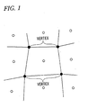
- the calculation data model need be generated such that a condition should be satisfied that adjacent divided domains always share the Vertex as shown in FIG. 1 .
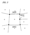
- the presence of Vertex not shared by adjacent divided domains is allowed as shown in FIG. 2 . This increases the flexibility of mesh generation in comparison with a finite element method.
- the calculation data model need be generated on conditions that unshared Vertex is located at least on an edge of adjacent divided domains and that, in general, the shape of the divided domain agrees with the element type for analysis set up in advance. Thus, it is hard to say that the flexibility of mesh generation is high.
- 3D shape data such as three-dimensional CAD (Computer Aided Design) data.
- 3D shape data is not data formed for numerical analysis.
- data is contained that indicates overlapping surfaces, surface intersection, gaps between surfaces, a small hole, and the like. That is, many conditions are included that are not suitable for generation of a calculation data model having Vertex and Connectivity.
- the 3D shape data need be modified or changed.
- the solver process calculates the volume of the divided domain, the area of the boundary surface, and the normal vector of the boundary surface, the amount of calculation increases further in the solver process so that computation load to the solver process increases further.
- the calculation data model can be generated in a short time. Nevertheless, the following problem arises.
- the analysis domain is defined basically by voxels (an orthogonal grid) all having the same size.
- the element size (the size of each divided domain) is set small in a domain where a higher accuracy of analysis is desired, so that the physical value calculation is achieved with precision in this domain. Further, the element size for the other domain is set large so that computation load for this domain is reduced.
- all voxels have basically the same size. Thus, when the voxels are set small, computation load becomes remarkably large.
- each analysis domain need be defined by arranging voxels (an orthogonal grid) having the same size.
- the analysis domain cannot be smooth near the boundary to an external domain and hence forms a stepwise shape in some cases. That is, even when an actual domain to be analyzed has an inclined plane, a curved surface, or the like, the domain is represented in a stepwise shape in the voxel data.
- the analysis domain shape in the voxel method becomes different from the actual domain shape to be analyzed. This degrades accuracy of analysis.
- a cut-cell method has been proposed that the step-like domain in the voxel data is cut along the inclined plane or the curved surface (boundary correction) present in the actual domain to be analyzed. Nevertheless, in this improved method, the boundary correction easily generates remarkably small divided domains. Then, when such small divided domains are generated, accuracy of analysis is degraded. Further, in this improved method, the cut cell generation and the solver process use Vertex.
- a voxel method without boundary correction does not require Vertex and the like. Nevertheless, limit is present in voxel generation, that is, in so-called mesh generation. That is, when sufficient accuracy of analysis is required, the number of voxels increases and the computation load in the solver process also increases. This causes a problem. Further, in an improved method of voxel method with boundary correction, Vertex becomes necessary as a result. Thus, an influence is caused from the geometric shape of the divided domains. As a result, remarkably enormous manual work requiring experience and a trial and error approach becomes necessary for the processing of divided domain generation near the boundary to the external domain. Thus, the shape data model cannot be generated in a short time.
- a particle method requires calculation of the linkage relation of a particular particle to other particles.
- particles present in the neighborhood of the particular particle need be searched for.
- this particle near neighbor algorithms is performed on all particles in principle.
- every particle moves time dependently and hence the linkage relation between particles varies always.
- the near neighbor algorithms need be performed at each time of change of the time in analysis. This causes an increase in the computation load.
- an attempt has been performed that particles on which the neighborhood search is to be performed are selected carefully so that the computation load in the near neighbor algorithms is reduced. Nevertheless, for example, when the number of particles is increased for the purpose of improvement of accuracy of analysis, the computation load increases in proportion to the square of the number of particles.
- a particle method when a physical phenomenon such as fluid, structure, heat, and diffusion based on the conservation law for a physical value is analyzed, the conservation is not sufficiently satisfied. For example, information concerning the area occupied on a boundary surface by a particle arranged such as to face the boundary surface between the analysis domain and the external domain is not present. Thus, even when a condition that heat is inputted through the boundary surface is desired to be placed, the amount of heat inputted to each particle is not recognized accurately. Thus, a precise quantitative value is not obtained.
- the present invention has been devised in view of the problems in the conventional methods for numerical analysis described above like a finite element method, a finite volume method, a voxel method, an improved technique of voxel method, and a particle method.
- An object of the present invention is to reduce work burden in generation of a calculation data model and to reduce computation load in solver process without causing degradation in accuracy of analysis.
- the present invention employs a configuration of a calculation method for physical value for calculating physical values in a numerical analysis method for numerically analyzing a physical phenomenon, comprising a physical value calculation step of calculating physical values in an analysis domain divided into a plurality of divided domains not limited to an orthogonal grid shape, wherein in the physical value calculation step, the physical values are calculated by using: a discretized governing equation that uses values not requiring coordinates (Vertex) of vertices of the divided domains and connectivity information (Connectivity) of the vertices and that is derived on the basis of a weighted residual method; and a calculation data model in which volumes of the divided domains and characteristic values of boundary surface indicating characteristics of boundary surfaces of adjacent ones of the divided domains are provided as the values not requiring coordinates (Vertex) of vertices of the divided domains and connectivity information (Connectivity) of the vertices.
- a discretized governing equation that uses values not requiring coordinates (Vertex) of vertices of the divided domains and
- the discretized governing equation used in the present invention is not conventional one expressed in a form containing values (Vertex and Connectivity) that set forth the geometric shape of each divided domain, and is one not requiring values that set forth the geometric shape of each divided domain.
- the discretized governing equation used in the present invention is obtained by intentionally stopping, in the middle, the process of deriving, on the basis of a weighted residual method, a conventional equation using values that set forth the geometric shape.
- Such a discretized governing equation used in the present invention is expressed in values not requiring the geometric shape of the divided domain (i.e., values not requiring Vertex and Connectivity), and then may be expressed in a form, for example, depending solely on the two of the volume of the divided domain and the characteristic value of boundary surface.
- the object to be analyzed is divided into minute domains as a premise.
- the discretized governing equation is derived on a premise that values setting forth the geometric shape of each minute domain, that is, Vertex and Connectivity, are used.
- the discretized governing equation used in the present invention is derived from a different and completely new way of thinking from the conventional art.
- the present invention is characterized by employing the discretized governing equation derived from such a new way of thinking.
- the method according to the present invention resolves the conventional problems without depending on the geometric shape, and provides various kinds of remarkable effects.
- the volume of the divided domain and the characteristic value of boundary surface are values not requiring Vertex and Connectivity that set forth a particular geometric shape of the divided domain.
- the values not requiring Vertex and Connectivity indicate values that can be defined without the use of Vertex and Connectivity.
- the volume of a divided domain is considered, plural possibilities are present for the geometric shape of the divided domain whose volume takes a predetermined value. That is, the geometric shape of the divided domain whose volume takes a predetermined value may be a cube or a sphere.
- the volumes of the divided domains may be defined by optimization calculation performed such that, for example, the volume of each divided domain should be proportional to the third power of the average distance from each adjacent divided domain as much as possible.
- the volume of the divided domain may be recognized as a quantity not requiring a particular geometric shape of the divided domain (a quantity not requiring Vertex and Connectivity).
- the characteristic value of boundary surface may be, for example, the area of the boundary surface, the normal vector of the boundary surface, or the contour length of the boundary surface.
- the characteristic value of boundary surface may be defined by optimization calculation performed such that the direction of the normal vector of the boundary surface is made close to the line segment that joins the control points of two adjacent divided domains (see FIG. 5 ) and that the total sum of the total boundary surface areas enclosing the divided domain should be proportional to the three-seconds power of the volume of the divided domain as much as possible.
- the characteristic value of boundary surface may be recognized as a quantity not requiring a particular geometric shape of the divided domain (a quantity not requiring Vertex and Connectivity).
- an analysis domain divided into a plurality of divided domains not limited to an orthogonal grid shape indicates that at least one of the plurality of divided domains constituting the analysis domain does not have an orthogonal grid shape. That is, the description indicates that the analysis domain contains a divided domain having a shape other than an orthogonal grid shape. Further, in the present invention, the description that "only values not requiring Vertex and Connectivity are used” indicates that values to be substituted into the discretized governing equation are only values not requiring Vertex and Connectivity.
- the calculation data model generated in the pre process does not have Vertex and Connectivity but have the volume of the divided domain, the characteristic value of boundary surface, and other auxiliary data (e.g., linkage information of the divided domains and control point coordinates which are described later).
- the calculation data model not having Vertex and Connectivity does not require the geometric shape of the divided domain, and hence can be generated without restriction caused by the geometric shape of the divided domain. Thus, restriction on correction work for the 3D shape data is also alleviated remarkably. Thus, the calculation data model not having Vertex and Connectivity can be generated far more easily than a calculation data model having Vertex and Connectivity. Thus, according to the present invention, work burden in generation of the calculation data model is reduced. Further, even when the present invention is used, in pre process, Vertex and Connectivity may be used. That is, in the pre process, the volume of the divided domain, the characteristics of boundary surface, and the like may be calculated by using Vertex and Connectivity.
- the present invention when used, in the pre process, restriction on the geometric shape of the divided domain is avoided.
- the divided domain may be changed into an arbitrary shape.
- the analysis domain can easily be fit to the actual domain to be analyzed without an increase in the number of divided domains.
- accuracy of analysis can be improved without an increase in the computation load.
- the density of distribution of the divided domains can also be changed arbitrarily.
- accuracy of analysis can also be improved further, with allowing an increase in the computation load to a necessary extent.
- the pre process generates a calculation data model having Vertex and Connectivity expressing the geometric shape of the divided domain. Then, the solver process calculates the volume of the divided domain and the characteristic value of boundary surface (the area of the boundary surface and the normal vector of the boundary surface) by using Vertex and Connectivity contained in the calculation data model, and then calculates physical values in each divided domain.
- the calculation data model i.e., a mesh
- the calculation data model need be generated within the restriction such as deformation and twist of the divided domain.
- the solver process calculates physical values by using Vertex and Connectivity contained in the calculation data model.
- the pre process need generate the calculation data model having Vertex and Connectivity expressing the geometric shape of the divided domain.
- enormous manual work arises in the calculation data model generation.
- a voxel method which is a conventional method for numerical analysis, as shown in FIG. 3 , at the time of calculating physical values in the solver process, Vertex and Connectivity are unnecessary.
- the shape of the divided domain is limited to a voxel.
- a problem arises that a boundary to an external domain has a stepwise shape.
- Vertex is used at the time of calculating the volume and the like of the divided domain.
- generation of the calculation data model is affected by the geometric shape of the divided domain.
- pre process generates a calculation data model having Vertex and Connectivity that define the geometric shape of the divided domain obtained by mesh dividing.
- the solver process requires linkage information (referred to as link, hereinafter) for the divided domain.
- link link
- the pre process generates a calculation data model having Vertex, Connectivity, and link.
- the calculation data model having Vertex, Connectivity, and link and a boundary condition, an initial condition, and the like necessary in the solver process are transferred from the pre process to the solver process.
- the solver process solves the discretized governing equation by using the Vertex, Connectivity, and the like contained in the transferred calculation data model, and thereby calculates physical values.
- the pre process generates a calculation data model having the volume of each divided domain arranged arbitrarily, the characteristic value of boundary surface (the area of the boundary surface and the normal vector of the boundary surface), and link. Further, as described later in detail, in the present invention, in some cases when necessary, the calculation data model is provided with the coordinates of the control point arranged in the inside of each divided domain. Then, in the present invention, as shown in FIG. 4 , the calculation data model having the volume of the divided domain, the characteristic value of boundary surface, and link (the coordinates of the control point, when necessary), a boundary condition, an initial condition, and the like are transferred from the pre process to the solver process. The solver process solves the discretized governing equation by using the volume of the divided domain, the characteristic value of boundary surface, and the like contained in the transferred calculation data model, and thereby calculates physical values.
- an essential difference of the present invention from the conventional finite volume method is that the solver process calculates physical values without the use of Vertex and Connectivity.
- This point is a remarkable feature of the present invention.
- This feature results from the fact that the solver process uses a discretized governing equation that uses only values not requiring Vertex and Connectivity.
- Vertex and Connectivity need not be transferred to the solver process.
- the pre process generates a calculation data model not having Vertex and Connectivity.
- the calculation data model can be generated far more easily. Thus, work burden in generation of the calculation data model is reduced.
- the shape of the analysis domain on which numerical analysis is to be performed varies time series, that is, the analysis domain includes a moving boundary.
- the divided domains need be moved and deformed in accordance with the moving boundary.
- calculation of physical values in a case that a moving boundary is included is achieved by a method that Vertex at every movement of the moving boundary is stored in advance or alternatively by a method that domain dividing is re-executed when calculability is lost owing to extreme deformation of the divided domain.
- calculation of physical values in a case that a moving boundary is included is achieved by a method that the volume of the divided domain, the characteristics of boundary surface, and the like in place of Vertex are calculated and stored in advance or alternatively by a method that domain dividing is re-executed.
- a plurality of calculation data models need be generated. Nevertheless, in the conventional finite volume method, in a situation that generation of merely a single calculation data model requires an enormous amount of work, generation of a plurality of models becomes unachievable within a range of practically available amount of work in many cases.
- the calculation data model need not have Vertex and Connectivity and the consistency in Vertex and Connectivity need not be considered in the domain dividing processing.
- the calculation data model can be calculated at a remarkably high speed.
- physical values in a case that a moving boundary is included are calculated easily.
- the link is information describing relation between divided domains in which physical values are exchanged with each other. Then, the divided domains whose relation is described in this link need not be spatially adjacent to each other. That is, they may be spatially apart from each other. Such link is not connected to Vertex or Connectivity. Thus, in comparison with Vertex and Connectivity, the link can be generated in a remarkably short time.
- the principle of the method for numerical analysis (referred to as the present numerical analysis method, hereinafter) using the present invention, that is, the principle that physical values can be calculated by using a discretized governing equation derived on the basis of a weighted residual method and by using the volume of the divided domain and the characteristic value of boundary surface is described in detail.
- a character surrounded by [] indicates a vector represented in a bold font in the drawings.
- the calculation data model in the present numerical analysis method is defined by using the volume of each divided domain obtained by dividing the analysis domain and the characteristic value of boundary surface indicating the characteristics of the boundary surface between adjacent divided domains.
- FIG. 5 is a conceptual diagram showing an example of a calculation data model of the present numerical analysis method as described above.
- the cells R 1 , R 2 , R 3 ... are divided domains obtained by dividing the analysis domain, and have volumes V a , V b , V c ..., respectively.
- the boundary surface E is a surface through which physical values are exchanged between the cell R 1 and the cell R 2 , and corresponds to the boundary surface in the present invention.
- the area S ab denotes the area of the boundary surface E, and is one of the characteristic values of boundary surface in the present invention.
- [n] ab denotes the normal vector of the boundary surface E, and is one of the characteristic values of boundary surface in the present invention.
- each control point is arranged at the position of the center of gravity of each of the cells R 1 , R 2 , R 3 ....
- each of the control points a, b, c... need not be arranged at the position of the center of gravity of each of the cells R 1 , R 2 , R 3 ....
- ⁇ denotes the distance from the control point a to the boundary surface E in a case that the distance from the control point a to the control point b is defined to be 1.
- ⁇ is a ratio indicating an internally dividing point where the boundary surface E is located on the line segment joining the control point a and the control point b.
- a boundary surface is present between every adjacent cells, rather than only between cell R 1 and cells R 2 . Then, the normal vector of the boundary surface and the area of the boundary surface are also provided for every boundary surface.
- the actual calculation data model is constructed as a data group having: arrangement data for the control points a, b, c...; volume data indicating the volumes V a , V b , V c ... of the cells R 1 , R 2 , R 3 ... where the control points a, b, c... are located; area data indicating the area of each boundary surface; and normal vector data indicating the normal vector of each boundary surface. That is, the calculation data model of the present numerical analysis method is defined by: the volumes V a , V b , V c ...
- the cells R 1 , R 2 , R 3 ... have the control points a, b, c..., respectively.
- the volumes V a , V b , V c ... of the cells R 1 , R 2 , R 3 ... may be recognized as the volumes of the spaces (control volumes) virtually occupied by the control points a, b, c..., respectively.
- the calculation data model of the present numerical analysis method has ratio data containing each ratio ⁇ indicating an internally dividing point where each boundary surface is located on the line segment joining the control points located on both sides of the boundary surface.
- t denotes time
- ⁇ denotes the density of fluid
- P denotes the pressure
- ⁇ denotes the coefficient of viscosity of the fluid
- V denotes the volume of the control volume
- ⁇ VdV denotes the integration with respect to the volume V
- S denotes the area of the control volume
- ⁇ SdS denotes the integration with respect to the area S
- [n] denotes the normal vector of S
- ⁇ / ⁇ n denotes the normal derivative.
- the density ⁇ and the coefficient of viscosity ⁇ of the fluid are set to be constant.
- the approach employing these constants here can be extended even for a case that the materials property values of the fluid vary with time, space, temperature, and the like.
- the area S ab of the boundary surface E is discretized so that each equation is transformed into an approximated equation in the form of an algebraic equation.
- the equation (3) is rewritten into the following equation (5) and the equation (4) is rewritten into the following equation (6).
- [n] ab , [u] ab , u iab , n iab , P ab , and ( ⁇ u i / ⁇ n) ab that have subscripts a and b are physical values on the boundary surface E between the control point a and the control point b.
- n iab is a component of [n] ab .
- m is the number of all control points in a linkage relation with the control point a (a relation of having a boundary surface in between).
- each of [u] ab , u iab , P ab , and ( ⁇ u i / ⁇ n) ab is obtained in approximation as a weighted average (a weighted average where upwind scheme is taken into consideration, in case of the advective term) of the physical value on the control point a and the control point b, and is determined depending on the distance and the direction between the control points a and b, the positional relation (the above-mentioned ratio ⁇ ) with the boundary surface E located between them, and the direction of the normal vector of the boundary surface E.
- a weighted average a weighted average where upwind scheme is taken into consideration, in case of the advective term
- [u] ab , u iab , P ab , and ( ⁇ u i / ⁇ n) ab are values independent of the geometric shape of the boundary surface E (i.e., values not requiring Vertex and Connectivity that set forth the cell shape).
- ⁇ ab defined by the equation (9) is a quantity (area/volume), and hence is a quantity independent of the geometric shape of the control volume (i.e., values not requiring Vertex and Connectivity that set forth the cell shape). That is, these equations (10) and (11) are operation formulas based on a weighted residual method in which the physical value can be calculated by using only values not requiring Vertex and Connectivity that set forth the cell shape.
- the flow velocity can be calculated in the physical value calculation completely without the use of the geometric shape of the control volume (i.e., Vertex and Connectivity that set forth the shape of the cell).
- the flow velocity can be calculated in the physical value calculation completely without using Vertex and Connectivity.
- the calculation data model need not have Vertex and Connectivity.
- restriction is not caused by the geometric shape of the cell and hence the shape of the cell can be set up arbitrarily.
- restriction on correction work for the 3D shape data can be alleviated remarkably as described above.
- the physical values such as [u] ab and P ab on the boundary surface E are interpolated in general by linear interpolation.
- the physical value at the control point a is denoted by ⁇ a
- the physical value at the control point b is denoted by ⁇ b
- the physical value ⁇ ab on the boundary surface E is obtained by the following equation (12).
- the physical value ⁇ ab can also be obtained by the following equation (13).
- the physical value on the boundary surface E can be calculated according to the equation (13) by using a weighted average corresponding to the distances from the control point a and from the control point b.
- equations for a continuum model contain 1st-order partial derivative (partial differentials) of first order as shown in the equation (1).
- the degree of differential is lowered by transforming a volume integration into a surface integral by using integration by parts, Gauss's divergence theorem, or the generalized Green's theorem.
- differential of 1st-order is made into differential of zero-order (a scalar value or a vector value).
- ⁇ the following equation (14) holds.
- the differential of 1st-order terms in the equation for continuum model are treated as scalar values or vector values on the boundary surface. Then, these values can be interpolated from the physical values at the individual control points by the above-mentioned linear interpolation or the like.
- a certain equation for continuum model contains a partial derivative of second order.
- the integrand in the equation (14) is differentiated by one-more order, the following equation (15) is obtained.
- the second-order differential term in the equation for continuum model is rewritten into the following equation (16) on the boundary surface E by using transformation of a volume integration into a surface integral.
- ⁇ / ⁇ n denotes the normal direction differential.
- ⁇ / ⁇ n ab denotes the [n] ab -direction differential. That is, by virtue of transformation of a volume integration into a surface integral, the second-order differential term in the equation for continuum model takes the form of a product between the normal direction differential of the physical value ⁇ (the differential in the direction of the normal [n] ab to S ab ) and the components n iab and n jab of [n].
- an inter-control-point vector [r] ab between the control point a and the control point b is defined as the following equation (18) on the basis of the position vector [r] a of the control point a and the position vector [r] b of the control point b.
- the partial derivatives in all terms contained in the linear partial differential equation can all be calculated from: the physical value ⁇ at the control point; ⁇ ab which is ⁇ on the boundary surface calculated according to the equation (12) or the equation (13); the inter-control-point distance obtained from the inter-control-point vector defined by the equation (18); the area S ab of the boundary surface E shown in the equation (5); and the components n iab and n jab of the normal vector shown in the equation (16).
- a term consisting of a product between ⁇ and the first-order partial derivative of ⁇ or a term consisting of the square of the first-order partial derivative, each of which is a non-linear term shown in the equation (20) can be obtained by numerical calculation by iteration calculation. That is, the iteration calculation may be performed in such a manner that ⁇ and the first-order partial derivative in each term are approximated by the calculated values obtained at the one-step prior iteration calculation. According to such a method, all non-linear terms in the partial differential equation can be obtained by numerical calculation.
- the description given above has been made for a particular case of equations for continuum model. However, as seen from the description given above, discretization not requiring Vertex and Connectivity is applicable to any other kinds of partial differential equations. Nevertheless, the conservation law requires another satisfaction condition. This point is described later.
- the physical value calculation does not require Vertex and Connectivity as described above.
- the flow velocity can be calculated by using the discretized governing equations shown in the equations (10) and (11) and completely not using the geometric shape of the control volume (i.e., the geometric shape of the cell).
- the volume of the control volume and the area and the normal vector of the boundary surface need not be calculated by not using the particular geometric shape of the control volume. That is, the solver process does not use Vertex and Connectivity.
- the above-mentioned normal vector may be replaced by the distance vector that joins the control volumes.
- the reason for this is described below.
- the normal vector [n] ab of the boundary surface E shown in FIG. 5 is in the same direction as the distance vector [r] ab that joins the control point a and the control point b
- the normal vector [n] is expressed as the following equation (21).
- the normal vector [n] ab of the boundary surface E is in the same direction as the distance vector [r] ab
- the equation (21) is substituted into the discretized governing equations shown in the equations (10) and (11)
- discretized governing equations in a case that the normal vector [n] ab is in the direction joining the control points a and b are obtained. That is, in a case that the boundary surface and the vector that joins the control points located on both sides of the boundary surface are orthogonal to each other, the normal vector in the discretized governing equations may be replaced by the distance vector.
- the normal vector [n] ab of the boundary surface E can be determined from only the position coordinates of the control point.
- the arbitrariness in the normal vector is lost, flexibility cannot be imparted to the orientation of the boundary surface in some cases.
- restriction arises on the setting of the volume of the control volume and the boundary surface at the time of generation of the calculation data model.
- the distance vector is necessary and hence the coordinates of the control point are necessary for the purpose of calculating the distance vector.
- the calculation data model need have the coordinate data of the control point or alternatively the distance vector data.
- the physical value calculation does not require Vertex and Connectivity.
- the cells R a , R b , R c , and R d are considered that divide the L-shaped passage into four sections.
- the control point a, b, c, and d arranged in the inside of the cells R a , R b , R c , and R d , respectively are located at the centers of the cells R a , R b , R c , and R d .
- the flow velocity vector on each boundary surface is assumed to be perpendicular to the boundary surface.
- V a is the volume of the cell R a (the volume of the control volume of the control point a)
- V b is the volume of the cell R b (the volume of the control volume of the control point b)
- V c is the volume of the cell R c (the volume of the control volume of the control point c)
- V d is the volume of the cell R d (the volume of the control volume of the control point d)
- ⁇ a is the density in the cell R a
- ⁇ b is the density in the cell R b
- ⁇ c is the density in the cell R c
- ⁇ d is the density in the cell R d
- Sa is the area of the boundary surface between the cell R a and the external domain
- S c is the area of the boundary surface between the cell R c and the external domain
- S d is the area of the boundary surface between the cell R d and the external domain
- S ab is the area of the boundary surface between the cell R a and the cell
- Discretization of the mass conservation equation is considered at the four control points a, b, c, and d (in the four cells R a , R b , R c , R d ) shown in FIG. 6 .
- the discretized governing equation obtained by discretizing the mass conservation equation is given in the later-described equation (43).
- the discretized governing equation at the control point a is shown in the following equation (22).
- the equation (30) indicates the fact that the difference between the in-following mass flux into the entire domain occupied by the control volumes of the control points a, b, c, and d and the out-flowing mass flux is equal to the change per unit time in the mean density (the mass change with respect to time) in the entire domain occupied by the control volumes of the control points a, b, c, and d. That is, the mass conservation equation discretized at each of the control points a, b, c, and d holds also in the domain occupied by the control volumes of all control points. That is, when each discretized governing equation in the control volume domain indicated by a control point is added up for all control points, an equation must be obtained that satisfies the conservation law for the entire domain of the analysis domain serving as a calculation object.
- the area of the boundary surface between the control points is assumed to be identical when viewed from the control point a side and when viewed from the control point b side.
- the mass flux ( ⁇ [n] ⁇ [u]) ⁇ S between the control points has an opposite sign of positive or negative and has the same absolute value on the control point a side and on the control point b side.
- the mass flux sum is canceled out into zero. That is, the equation (31) indicates that the difference between the in-flowing mass and the out-flowing mass in the entire domain to be calculated is equal to the mass change per unit time in the entire domain.
- the equation (31) serves as the mass conservation equation in the entire analysis domain.
- Equation (33) indicates that the polyhedron constituting the control volume forms a closure space. This equation (33) holds even when a part of the polyhedron constituting the control volume is concave.
- the equation (33) holds also for a triangle in two dimensions. Further, when limit is taken such that one surface of the polyhedron is made into an infinitesimal surface dS and then m is made ⁇ , the following equation (34) is obtained. This holds even for a closure curved surface object as shown in FIG. 9 .
- the condition that the equation (33) holds is necessary for a condition that Gauss's divergence theorem or the generalized Green's theorem shown in the equation (14) holds. Then, the generalized Green's theorem is a theorem providing the basis for the discretization of the continuum. Thus, in a case that a volume integration is changed into a surface integral according to the theorem of green and then discretization is performed, the condition that the equation (33) holds is indispensable in order that the conservation law should be satisfied.
- the calculation data model need be generated such that these conditions are satisfied.
- the cell shape can be deformed arbitrarily.
- the calculation data model can easily be generated such that the above-mentioned three conditions are satisfied.
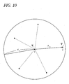
- the MPS method is a technique that particles present within a sphere of radius r e set up appropriately are detected, then a linkage relation with each particle is established, and then calculation is performed. For example, as shown in FIG. 10 , when a plurality of particles j are present around a particle i, the Laplacian ( ⁇ 2 ⁇ ) i for the particle i is approximated as the following equation (35).
- ⁇ i denotes the physical value at the particle i
- ⁇ j denotes the physical value at the particle j
- [r] ij denotes the distance vector from the particle i to the particle j.
- d in the equation (35) denotes the constant indicating the dimension, and hence is equal to three in a case of three dimensions.
- ⁇ (r) in the equation (35) is a weight function expressed by the following equation (36).
- m in the equation (35) is the number of particles in the linkage relation.
- the dimension is identical (1/distance) in the left side and in the right-hand side of the equation (39).
- the formulation of the MPS method may be interpreted as a technique that the quantity of (area/volume) (i.e., the ratio defined by the equation (9)) in the right-hand side shown in the following equation (40) is calculated from only the distance between two particles i and j.
- the particles move in association with the change of time.
- near neighbor algorithms need be performed that particles present within the above-mentioned sphere of radius r e are detected.
- This causes large computation load in the physical value calculation.
- the control volume and the control point do not move even when time varies.
- the physical value calculation is achieved without near neighbor algorithms. This reduces computation load in the physical value calculation in comparison with the MPS method.
- the processing of defining the arrangement relation of the control volumes and the control points is performed only once in the beginning.
- the description given above has been made for an example of physical value calculation using a discretized governing equation derived from the Navier-Stokes equations and the continuity equation on the basis of a weighted residual method.
- the discretized governing equation to be used in the present numerical analysis method is not limited to this. That is, any discretized governing equation that is derived from various kinds of equations (such as the mass conservation equation, the equation for conservation of momentum, the equation for conservation of energy, the advection diffusion equation, and the wave equation) on the basis of a weighted residual method and that can calculate physical values by using only values not requiring Vertex and Connectivity may be used in the present numerical analysis method.
- a discretized governing equation that uses only values not requiring Vertex and Connectivity can be derived from the mass conservation equation, the equation for conservation of momentum, the equation for conservation of energy, the advection diffusion equation, and the wave equation on the basis of a weighted residual method, that is, the fact that the present numerical analysis method can employ other governing equations.
- ⁇ ab and [n] ab that have subscripts a and b are physical values on the boundary surface E between the control point a and the control point b.
- m is the number of all control points in a linkage relation with the control point a (a relation of having a boundary surface in between).
- Such an equation (46) is an equation that is derived on the basis of a weighted residual method and that uses only values not requiring Vertex and Connectivity. Thus, such an equation may be used as a discretized governing equation in the present numerical analysis method.
- the discretized governing equation used in the present invention is obtained by intentionally stopping, in the middle, the process of deriving, on the basis of a weighted residual method, a conventional equation using values that set forth the geometric shape. That is, the equation (46) is obtained in the process that the mass conservation equation is derived as an equation that uses Vertex and the like, on the basis of a weighted residual method.
- FIG. 12 is a schematic diagram showing a cell having a two-dimensional triangular shape. The area, the length of side, and the normal vector of the triangle a in FIG. 12 are shown in the following table.
- symbol ⁇ in the following table denotes a cross product.
- [r] i is the position vector (coordinates) of the vertex (Vertex) i
- symbol ⁇ denotes the cross product of vectors.
- ⁇ ab and p are fixed
- [r] ij is equal to [r] j -[r] i
- [r] 4 is identical to [r] 1 .
- the other values are similar to those in the equation (41). Further, the summation notation is applied for the subscripts j.
- This equation (47) is a basic equation for a stress field in a structure, a material, a fluid, or the like.
- Equation (52) C is the concentration of the substance C
- ⁇ c is the diffusion coefficient of the substance C
- q c is the source (sink) term for the substance C
- ⁇ is the density of the continuum
- u i denotes the deformation rate of the continuum.
- values such as Ca having subscript a are physical values at the control point a.
- Values such as C ab having subscripts ab are physical values on the boundary surface between the control point a and the control point b.
- Equation (54) U is the internal energy of the continuum, q i is the heat flux vector, r is the heat source and the source (sink) term of thermal energy, ⁇ ij is the stress tensor, and D ij is the deformation rate tensor.
- the term of double tensor product of ⁇ ij ⁇ D ij is referred to as a stress power.
- the summation notation is applied for the subscripts i and j. Then, when the equation (54) is integrated on the basis of a weighted residual method and then discretized and transformed into a discretized governing equation, the following equation (55) is obtained.
- Equation (56) u is the amplitude or displacement, and ⁇ is velocity of propagation of the wave. Then, when the equation (56) is integrated on the basis of a weighted residual method and then discretized and transformed into a discretized governing equation, the following equation (57) is obtained.
- equations (46), (51), (53), (55), and (57) are equations that are derived on the basis of a weighted residual method and that can calculate physical values by using only values not requiring Vertex and Connectivity.
- equations may be used as a discretized governing equation in the present numerical analysis method.
- the present numerical analysis method can be applied to numerical analysis for a stationary or non-stationary phenomenon in fluid dynamics, heat conduction, advection diffusion, structural mechanics, wave, or a combination of these.
- the numerical analysis can be performed in a state that components designed in different coordinate systems are built up easily. This is because in the present numerical analysis method, in contrast to the element used in a finite element method, the particular geometric shape of the control volume is not necessary and because the "distance" between two adjacent control points need not be a distance in the absolute coordinate system and may be a "calculative distance".
- the present numerical analysis method as shown in FIG. 13 , in a case that numerical analysis is desired to be performed in a state that components A, B, and C designed in different coordinate systems are built up, the numerical analysis can be performed without matching the coordinate systems of these components.
- a method for numerical analysis referred to as a general finite element method is a technique that completely inhibits intersection between elements as shown in FIG. 14 or 15 .
- a finite element method in application software used in a finite element method, when intersection between elements is detected, an error is outputted. Then, as described above, such situation in a finite element method causes remarkably large work burden in generation of a calculation data model.
- intersection is allowed in linkage between control points. This is because informational values such as the volume of the control volume occupied by each control point (the volume of the divided domain), the area of the boundary surface, and the normal vector of the boundary surface need not have a particular geometric shape.
- a calculation method for physical value a numerical analysis method, a calculation program for physical value, a numerical analysis program, a calculation device for physical value, and a numerical analysis device according to the present invention.
- the following description is given for an embodiment of a numerical analysis method including a calculation method for physical value according to the present invention, a numerical analysis program including a calculation program for physical value according to the present invention, and a numerical analysis device including a calculation device for physical value according to the present invention.
- the following embodiment is given for a case that the flow velocity of air in a vehicle cabin space is calculated by numerical analysis.
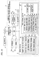
- FIG. 16 is a block diagram schematically showing a hardware configuration of a numerical analysis device A according to the present embodiment.
- the numerical analysis device A according to the present embodiment is constructed from a computer such as a personal computer and a workstation, and has a CPU 1, a memory device 2, a DVD (Digital Versatile Disc) drive 3, an input device 4, an output device 5, and a communication device 6.
- a computer such as a personal computer and a workstation
- the CPU 1 is electrically connected to the memory device 2, the DVD drive 3, the input device 4, the output device 5, and the communication device 6, and processes signals inputted from these various kinds of devices and then outputs the processing results.
- the memory device 2 is constructed from an external memory device such as a memory and an internal memory device such as a hard disk drive, and stores information inputted from the CPU 1 and outputs the stored information in response to an instruction inputted from the CPU 1. Then, the memory device 2 according to the present embodiment has a memory device for programs 2a and a data storage section 2b.
- the memory device for programs 2a stores a numerical analysis program P.
- This numerical analysis program P is an application program executed on a predetermined OS, and causes the numerical analysis device A constructed from a computer according to the present embodiment to perform numerical analysis. Then, the numerical analysis program P causes the numerical analysis device A according to the present embodiment to serve as, for example, calculation data model generating means and physical value calculating means. Then, as shown in FIG. 16 , the numerical analysis program P has a pre process program P1, a solver process program P2, and a post process program P3.
- the pre process program P1 causes the numerical analysis device A according to the present embodiment to execute pre process necessary for execution of solver process, and causes the numerical analysis device A according to the present embodiment to serve as calculation data model generating means so as to generate a calculation data model. Further, the pre process program P1 causes the numerical analysis device A according to the present embodiment to execute setting of conditions necessary for execution of the solver process and further to execute generation of a solver input data file F collecting the calculation data model and the set-up conditions described above.
- the pre process program P1 first causes the numerical analysis device A according to the present embodiment to acquire 3D shape data including a vehicle cabin space and then execute generation of an analysis domain expressing the vehicle cabin space included in the acquired 3D shape data.
- the solver process uses the discretized governing equation described in the above-mentioned method for numerical analysis using the present invention (a discretized governing equation that uses only values not requiring Vertex and Connectivity and that is derived on the basis of a weighted residual method).
- the shape of the divided domain and the shape of the analysis domain can be changed arbitrarily on condition that the conservation law is satisfied.
- the work of correction or change of the vehicle cabin space included in the 3D shape data is achieved by simple lapping or the like.
- the pre process program P1 according to the present embodiment causes the numerical analysis device A according to the present embodiment to lap with minute closed surfaces the vehicle cabin space included in the acquired 3D shape data so as to execute lapping for repairing a hole or a gap present in the vehicle cabin space.
- the pre process program P1 causes the numerical analysis device A according to the present embodiment to generate divided domains having the same size and execute generation of an analysis domain including the entire domain of the cabin space having undergone the lapping.
- the pre process program P1 causes the numerical analysis device A according to the present embodiment to cut off domains falling outside the cabin space among the divided domains generated in the same size so as to execute generation of an analysis domain representing the cabin space. Also at this time, since the solver process uses the above-mentioned discretized governing equation, domains falling outside the cabin space in the analysis domain can be cut off easily. This avoids a situation that a boundary to the outer space has a stepwise shape like in a voxel method. Further, in contrast to a cut-cell method of voxel method, generation of an analysis domain near a boundary to the outer space does not require special correction or processing that causes remarkably enormous manual work requiring experience and a trial and error approach.
- the present embodiment does not have a problem associated with the processing for a boundary to the outer space.
- a gap between the cabin space and the cut-off domain is filled with divided domains having a new arbitrary shape so that the analysis domain is constructed from divided domains whose shapes are not limited to an orthogonal grid shape. Further, the analysis domain is filled with the divided domains without overlapping.
- the pre process program P1 causes the numerical analysis device A according to the present embodiment to execute the processing of virtually arranging one control point in the inside of each divided domain contained in the generated analysis domain representing the cabin space and then store the arrangement information concerning the control points and the volume data concerning the control volume occupied by each control point. Further, when causing the numerical analysis device A according to the present embodiment to serve as calculation data model generating means, the pre process program P1 causes the numerical analysis device A according to the present embodiment to execute calculation of the area and the normal vector of each boundary surface which is a boundary surface between divided domains described above and then store the area and the normal vector of the boundary surfaces.
- the pre process program P1 when causing the numerical analysis device A according to the present embodiment to serve as calculation data model generating means, the pre process program P1 causes the device to generate the linkage information (Link) concerning the control volumes (control points) and then store the Link. Then, the pre process program P1 causes the numerical analysis device A according to the present embodiment to collect the volume of the control volume occupied by the above-mentioned individual control point, the area and the normal vector of the boundary surface, the arrangement information (the coordinates) concerning the control points (i.e., divided domains) and the Link, and then generate a calculation data model.
- Link linkage information
- the pre process program P1 causes the numerical analysis device A according to the present embodiment to collect the volume of the control volume occupied by the above-mentioned individual control point, the area and the normal vector of the boundary surface, the arrangement information (the coordinates) concerning the control points (i.e., divided domains) and the Link, and then generate a calculation data model.
- the pre process program P1 causes the device to perform setting of property, setting of boundary conditions, setting of initial conditions, and setting of calculation conditions.
- the materials property values indicate the density, the coefficient of viscosity, and the like of air in the cabin space.
- the boundary conditions set forth rules used at the time of exchange of a physical value between control points and are, in the present embodiment, a discretized governing equation based on the Navier-Stokes equations shown in the equation (10) given above and a discretized governing equation based on the continuity equation shown in the equation (11).
- boundary conditions include information specifying divided domains facing a boundary surface between the cabin space and the outer space.
- the initial conditions specify physical values in the beginning of execution of the solver process, and are initial values for the flow velocity of each divided domain.
- the calculation conditions are conditions concerning the calculation in the solver process and are, for example, the number of iteration and a criterion for convergence.
- the pre process program P1 causes the numerical analysis device A according to the present embodiment to form a GUI (Graphical User Interface). More specifically, the pre process program P1 causes the display 5a provided in the output device 5 to display graphics, and generates a state that operation is allowed through the keyboard 4a and the mouse 4b provided in the input device 4.
- GUI Graphic User Interface
- the solver process program P2 (a calculation program for physical value) causes the numerical analysis device A according to the present embodiment to execute solver process, and causes the numerical analysis device A according to the present embodiment to serve as a calculation device for physical value. Then, when causing the numerical analysis device A according to the present embodiment to serve as physical value calculating means, the solver process program P2 causes the device to perform physical value calculation on the physical values in the analysis domain by using the solver input data file F containing the volume of the control volume, the area of the boundary surface, and the normal vector provided in the calculation data model.
- the solver process program P2 causes the numerical analysis device A according to the present embodiment to execute generation of a discretization coefficient matrix for the Navier-Stokes equations and the continuity equation contained in the solver input data file F and then execute generation of a data table for matrix generation.
- the solver process program P2 causes the numerical analysis device A according to the present embodiment to execute build-up of a large sparse matrix equation for matrix calculation shown in the following equation (58), by using the discretized governing equation based on the Navier-Stokes equations shown in the equation (10) described above and the discretized governing equation based on the continuity equation shown in the equation (11) described above.
- [A] denotes a large sparse matrix
- [B] denotes a boundary condition vector
- [X] denotes a solution.
- the solver process program P2 causes the numerical analysis device A according to the present embodiment to execute incorporation of the additional condition into the matrix equation. Then, the solver process program P2 causes the numerical analysis device A according to the present embodiment to execute calculation of the solution of the matrix equation by a CG method (conjugate gradient method) or the like, update of the solution by using the following equation (59), and judgment of the convergence condition, and thereby to acquire a final calculation result.
- CG method conjuggate gradient method
- the post process program P3 causes the numerical analysis device A according to the present embodiment to execute post process, and causes the numerical analysis device A according to the present embodiment to execute processing based on the calculation result acquired in the solver process. More specifically, the post process program P3 causes the numerical analysis device A according to the present embodiment to execute visualization process and extraction processing for the calculation result.
- the visualization process is, for example, the processing of causing the output device 5 to output a display of contour of cross section, a vector display, an equi-contour surface display, and an animation display.
- the extraction processing is the processing of causing the output device 5 to extract quantitative values in the domain specified by an operator and then output them as numerical values or a graph or alternatively to extract the quantitative values in the domain specified by the operator and then output them in the form of a file.
- the post process program P3 causes the numerical analysis device A according to the present embodiment to execute automatic report generation, calculation residual display, and analysis.
- the data storage section 2b stores: a solver input data file F containing a calculation data model M, data of boundary conditions D1 describing the boundary conditions, calculation condition data D2 describing the calculation conditions, materials property data D3 describing the materials property values, and initial condition data D4 describing initial conditions; 3D shape data D5; calculation result data D6; and the like. Further, the data storage section 2b temporarily stores intermediate data generated in the course of processing by the CPU 1.
- the DVD drive 3 is constructed such that a DVD medium X can be inserted therein. Then, in response to an instruction inputted from the CPU 1, the DVD drive outputs the data stored in the DVD medium X.
- the numerical analysis program P is stored in the DVD medium X. Then, in response to an instruction inputted from the CPU 1, the DVD drive 3 outputs the numerical analysis program P stored in the DVD medium X.
- the input device 4 is a man-machine interface between the numerical analysis device A according to the present embodiment and an operator, and has a keyboard 4a and a mouse 4b serving as pointing devices.
- the output device 5 outputs in a visualized manner a signal inputted from the CPU 1, and has a display 5a and a printer 5b.
- the communication device 6 performs data transfer between the numerical analysis device A according to the present embodiment and an external device such as a CAD device C, and is electrically connected to a network B such as an intra-company LAN (Local Area Network).
- a network B such as an intra-company LAN (Local Area Network).
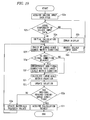
- the numerical analysis method according to the present embodiment is constructed from pre process (step S1), solver process (step S2), and post process (step S3).
- the CPU 1 extracts from the DVD medium X the numerical analysis program P stored in the DVD medium X inserted into the DVD drive 3, and then stores the program into the memory device for programs 2a of the memory device 2. Then, when a signal instructing the start of numerical analysis is inputted through the input device 4, the CPU 1 executes numerical analysis on the basis of the numerical analysis program P stored in the memory device 2.
- the CPU 1 executes pre process (step S1) on the basis of the pre process program P1 stored in the memory device for programs 2a, then executes solver process (step S2) on the basis of the solver process program P2 stored in the memory device for programs 2a, and then executes post process (step S3) on the basis of the post process program P3 stored in the memory device for programs 2a.
- the numerical analysis device A when the CPU 1 executes the pre process (step S1) on the basis of the pre process program P1, the numerical analysis device A according to the present embodiment serves as calculation data model generating means.
- the numerical analysis device A when the CPU 1 executes the solver process (step S2) on the basis of the solver process program P2, the numerical analysis device A according to the present embodiment serves as physical value calculating means.
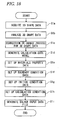
- FIG. 18 is a flow chart showing the pre process (step S1).
- the CPU 1 when the pre process (step S1) is started, the CPU 1 causes the communication device 6 to acquire the 3D shape data D5 including the vehicle cabin space, from the CAD device C via the network B (step S1a).
- the CPU 1 stores the acquired 3D shape data D5 into the data storage section 2b of the memory device 2.
- the CPU 1 performs analysis of the 3D shape data D5 acquired at step S1a (step S1b) so as to detect mutually overlapping curved surfaces, mutually intersecting curved surfaces, a gap between curved surfaces, a small hole, and the like contained in the 3D shape data D5 stored in the data storage section 2b.
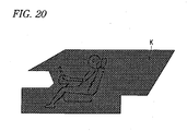
- the CPU 1 executes correction or change processing for the 3D shape data D5 acquired at step S1a (step S1c). More specifically, as shown in FIG. 20 , the CPU 1 performs lapping by using minute closed surfaces onto the cabin space K included in the 3D shape data D5, so as to correct the 3D shape data D5 for the cabin space such that mutually overlapping curved surfaces, mutually intersecting curved surfaces, a gap between curved surfaces, a small hole, and the like are eliminated.
- the CPU 1 generates a GUI.
- an instruction e.g., an instruction specifying a lapping domain
- the CPU executes correction or change processing where the instruction is reflected.
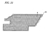
- the CPU 1 executes the generation of the calculation data model (step S1d). More specifically, as shown in FIG. 21 , on the basis of the 3D shape data D5 corrected or changed at step S1c, the CPU 1 first executes generation of an analysis domain K1 that includes the entire domain of the cabin space and that is divided uniformly with divided domains having the same shape (an orthogonal grid).
- the analysis domain K1 is divided with divided domains having the same shape for the purpose of shortening the time.
- the divided domains constituting the analysis domain K1 need not have the same shapes and may have arbitrary shapes. Then, as shown in FIG.
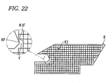
- the CPU 1 deletes divided domains falling outside the cabin space K so that the analysis domain K is accommodated inside the cabin space K without falling outside.
- a gap Y is formed between a boundary surface K1F of the analysis domain K1 and a boundary surface KF of the cabin space K.
- the CPU 1 fills the gap Y with new divided domains RA that constitute a part of the analysis domain.
- a calculation data model not having Vertex and Connectivity is generated.
- the calculation data model generation can be performed without restriction on the geometric shape of each divided domain. That is, at the time of generation of a calculation data model, the divided domains constituting the analysis domain K1 may have arbitrary shapes.
- the CPU 1 may arbitrarily set up the shapes of the divided domains RA as shown in the enlarged view of FIG. 23 .
- the CPU 1 virtually arranges one control point in the inside of each divided domain included in the analysis domain representing the cabin space.
- the CPU 1 calculates the centroid of the divided domain and then virtually arranges one control point to each centroid.
- the CPU 1 calculates the arrangement information concerning the control points and the volume of the control volume occupied by each control point (the volume of the divided domain where the control point is arranged) and then temporarily stores these into the data storage section 2b of the memory device 2.
- the CPU 1 calculates the area and the normal vector of each boundary surface which is a boundary surface between divided domains, and then temporarily stores the areas and the normal vectors of these boundary surfaces into the data storage section 2b of the memory device 2.
- the CPU 1 generates Link and then temporarily stores the Link into the data storage section 2b of the memory device 2. Then, the CPU 1 brings into the form of a database the arrangement information concerning the control points, the volume of the control volume occupied by each control point, the area and the normal vector of each boundary surface, and the Link which have been stored in the data storage section 2b, so as to generate a calculation data model M and then store the generated calculation data model into the data storage section 2b of storage section 2.
- the analysis domain including the cabin space is divided uniformly into divided domains having the same shape, then divided domains falling outside the cabin space are deleted, and then a gap having occurred between the analysis domain and the cabin space is filled with new divided domains so that a final analysis domain K2 is generated.
- a state is realized that the entire domain of the cabin space is filled with divided domains without overlapping.
- the calculation data model satisfies the above-mentioned three conditions (a) to (c) necessary for satisfying the conservation law.
- step S1d a configuration is employed that divided domains are generated first, then control points are arranged, and then a volume of the divided domain is assigned to each control point.
- control points may first be arranged to the analysis domain, and then a volume may be assigned to each control point.
- a weight is imparted to each control point on the basis of the radius causing collision with other control point or alternatively on the basis of the distance to a control point in linkage relation (related by Link).
- the weight of the control point i is w i
- the reference volume is V +
- the volume V i assigned to the control point i is as shown in the following equation (60).
- the volume to be assigned to each control point is obtained from the equations (61) and (62).
- the volumes of divided domains to be provided in the calculation data model are obtained without using Vertex and Connectivity.
- the CPU 1 in the generation of the calculation data model (step S1d), the CPU 1 generates a GUI. Then, when an instruction (i.e., an instruction specifying the density of the divided domain or an instruction specifying the shape of the divided domain) is inputted through the GUI, the CPU executes processing in which the instruction is reflected.
- an instruction i.e., an instruction specifying the density of the divided domain or an instruction specifying the shape of the divided domain
- the CPU executes processing in which the instruction is reflected.
- the CPU 1 checks satisfaction of the three conditions necessary for satisfying the conservation law which is stored in the numerical analysis program. Then, when the instruction inputted through the GUI violates the conditions, the CPU displays the situation on the display 5a.
- the CPU 1 performs setting of the materials property data (step S1e). Specifically, the CPU 1 displays an input screen for materials property values onto the display 5a through the GUI. Then, signals indicating materials property values inputted through the keyboard 4a or the mouse 4b are temporarily stored as the materials property data D3 into the data storage section 2b, so that the materials property values are set up.
- the materials property values mentioned here indicate the characteristic values of the fluid (i.e., air) in the cabin space, like the density, the coefficient of viscosity, and the like of air.
- the CPU 1 performs setting of the data of boundary conditions (step S1f). Specifically, the CPU 1 displays an input screen for boundary conditions onto the display 5a through the GUI. Then, signals indicating boundary conditions inputted through the keyboard 4a or the mouse 4b are temporarily stored as the data of boundary conditions D1 into the data storage section 2b, so that the data of boundary conditions is set up.
- the boundary conditions mentioned here indicate: a discretized governing equation that governs the physical phenomenon in the cabin space; information that specifies control points facing the boundary surface between the cabin space and the outer space; the conditions for heat conduction of heat between the cabin space and the outer space; and the like.
- its object is to obtain the flow velocity in the cabin space by numerical analysis.
- the above-mentioned discretized governing equations are the discretized governing equation (10) based on the above-mentioned Navier-Stokes equations and the discretized governing equation (11) based on the continuity equation.
- these discretized governing equations are selected, for example, by a method that a plurality of discretized governing equations stored in advance in the numerical analysis program P are displayed on the display 5a and then an operator selects any one or ones from the displayed plurality of discretized governing equations by using the keyboard 4a and the mouse 4b.
- the CPU 1 performs setting of the initial condition data (step S1g). Specifically, the CPU 1 displays an input screen for initial conditions onto the display 5a through the GUI. Then, signals indicating initial conditions inputted through the keyboard 4a or the mouse 4b are temporarily stored as the initial condition data D4 into the data storage section 2b, so that the initial condition data is set up.
- the initial condition mentioned here indicates the initial flow velocity at each control point (each divided domain).
- the CPU 1 performs setting of the calculation condition data (step S1h). Specifically, the CPU 1 displays an input screen for calculation conditions onto the display 5a through the GUI. Then, signals indicating calculation conditions inputted through the keyboard 4a or the mouse 4b are temporarily stored as the calculation condition data D2 into the data storage section 2b, so that the calculation condition data is set up.
- the calculation conditions mentioned here indicate conditions for the calculation in the solver process (step S2), like the number of iteration and criterion for convergence.
- the CPU 1 performs generation of a solver input data file F (step S1i). Specifically, the CPU 1 stores in the solver input data file F the calculation data model M generated at step S1d, the materials property data D3 set up at step S1e, the data of boundary conditions D1 set up at step S1f, the initial condition data D4 set up at step S1g, and the calculation condition data D2 set up at step S1h, and thereby generates the solver input data file F.
- the solver input data file F is stored into the data storage section 2b.
- step S2 the CPU 1 executes the solver process (step S2) shown in the flow chart of FIG. 19 on the basis of the solver process program P2.
- step S2a the solver input data file F generated in the pre process (step S1) (step S2a).
- the solver input data file F is already stored in the data storage section 2b. Thus, this step S2a may be skipped.
- step S1 and the solver process (steps S2) are executed by mutually different devices, the solver input data file F conveyed through a network or a removable disk need be acquired and hence the present step S2a need be executed.
- the CPU 1 judges the conformity of the solver input data (step S2b).
- the solver input data is data stored in the solver input data file F, and includes the calculation data model M, the data of boundary conditions D1, the calculation condition data D2, the materials property data D3, and the initial condition data D4.
- the CPU 1 analyzes whether all kinds of solver input data necessary for the execution of physical value calculation in the solver process are stored in the solver input data file F, and thereby judges the conformity of the solver input data.
- the CPU 1 displays an error on the display 5a (step S2b), and then displays a screen through which data of the inconformity part is inputted.
- the CPU 1 performs adjustment of the solver input data (step S2c), and then executes step S2a again.
- the CPU 1 executes initial calculation (step S2e). Specifically, the CPU 1 generates a discretization coefficient matrix from the discretized governing equations (i.e., the discretized governing equation (10) based on the Navier-Stokes equations and the discretized governing equation (11) based on the continuity equation) stored in the data of boundary conditions D1, and then generates a data table for matrix calculation so as to perform the initial calculation.
- the discretized governing equations i.e., the discretized governing equation (10) based on the Navier-Stokes equations and the discretized governing equation (11) based on the continuity equation
- the CPU 1 performs build-up of a large sparse matrix equation (step S2f). Specifically, by using the discretized governing equation (10) based on the Navier-Stokes equations and the discretized governing equation (11) based on the continuity equation, the CPU 1 performs build-up of the large sparse matrix equation for matrix calculation shown in the above-mentioned equation (58).
- the CPU 1 judges whether an additional condition such as incompressibility and contact is placed on the discretized governing equation.
- Such an additional condition is, for example, stored as data of boundary conditions in the solver input data file F.
- the CPU 1 executes build-in of the additional condition into the large matrix equation (step S2h), and then executes calculation of the large matrix equation (step S2i).
- the CPU 1 does not execute build-in of an additional condition into the large matrix equation (step S2h), and then executes calculation of the large matrix equation (step S2i).
- the CPU 1 solves the large matrix equation, for example, by a CG method (conjugate gradient method), and then performs update of the solution by using the above-mentioned equation (59) (step S2j).
- the CPU 1 judges whether the residual of the equation (59) has reached the convergence condition (step S2g). Specifically, the CPU 1 calculates the residual of the equation (59), then compares the result with the convergence condition contained in the calculation condition data D2, and then judges whether the residual of the equation (59) has reached the convergence condition. Then, when it is judged that the residual has not yet reached the convergence condition, the CPU 1 performs update of the materials property values, and then executes step S2g again. That is, the CPU 1 repeats steps S2f to S2g with performing the update of the materials property values until the residual of the equation (59) reaches the convergence condition.
- the CPU 1 acquires the calculation result (step S21). Specifically, the CPU 1 stores the solution of the physical value calculated at the immediately preceding step S2i, as the calculation result data into the data storage section 2b so as to achieve the acquisition of the calculation result.
- step S2 the flow velocity of air in the cabin space is calculated.
- solver process (step S2) corresponds to the calculation method for physical value of the present invention.
- the CPU 1 executes post process (step S3) on the basis of the post process program P3.
- the CPU 1 in response to an instruction inputted through the GUI, the CPU 1 generates, for example, data of contour of cross section, vector data, equi-contour surface data, and animation data from the calculation result data, and then visualizes the data on the output device 5.
- the CPU 1 extracts quantitative values (a calculation result) in a part of the cabin space and converts them in the form of numerical values or a graph, then visualizes the numerical values and the graph on the output device 5, and further outputs the numerical values and the graph collectively in the form of a file.
- the CPU 1 performs, for example, automatic report generation, calculation residual display, and analysis, and then outputs the result.
- the pre process generates the calculation data model M having the volume of the control volume and the area and the normal vector of the boundary surface, and then the solver process calculates the physical value in each control volume by using the volume of the control volumes and the area and the normal vector of the boundary surface contained in the calculation data model M. That is, as described in the above-mentioned method for numerical analysis, according to the numerical analysis device A, the numerical analysis method, and the numerical analysis program of the present embodiment, numerical analysis is achieved without generating a calculation data model having Vertex and Connectivity. This also remarkably alleviates restriction on correction or change work for the 3D shape data.
- the calculation data model M can be generated far more easily than a calculation data model having Vertex and Connectivity.
- work burden is reduced in generation of the calculation data model.
- the solver process in contrast to a conventional method for numerical analysis, the solver process need not calculate the volume of the control volume and the area and the normal vector of the boundary surface by using Vertex and Connectivity. This reduces computation load in the solver process.
- work burden is reduced in generation of the calculation data model and computation load is reduced in the solver process.
- the analysis domain is filled with divided domains without overlapping.
- the calculation data model M according to the present embodiment can be easily generated from mesh data used in a conventional finite volume method or a finite element method, particle data used in a conventional particle method, or simple point group data. Even in this case, correction of divided domains in the boundary area with the outer space is unnecessary in contrast to a voxel method.
- each element may be recognized as a divided domain according to the present embodiment (a control volume occupied by a control point) so that the generation is achieved easily.
- a closed space obtained by filling up the analysis domain with closed spaces each surrounding a control point arranged in the analysis domain may be recognized as a divided domain (a control volume occupied by a control point) according to the present embodiment so that the generation is achieved easily.
- the numerical analysis device A, the numerical analysis method, and the numerical analysis program of the present embodiment as described above, work burden for the calculation data model in the pre process is reduced remarkably and computation load in the solver process is also reduced.
- the present invention permits physical value calculation within a practical time by repeating the pre process and the solver process at each time that shape change occurs in the analysis domain, as shown in the flow chart of FIG. 24 .
- the weighted average of the flow velocities at the control points located on both sides of the boundary surface calculated by using a weight corresponding to the ratio of the distances from the control points to the boundary surface may be adopted as the flow velocity on the boundary surface.
- the mean of the flow velocities at the control points located on both sides of the boundary surface is simply adopted as the flow velocity on the boundary surface, the flow velocity in the cabin space can be calculated more precisely.
- the calculation data model need have the data of the ratio ⁇ that indicates the internally dividing point where the boundary surface is located on the line segment that joins the control points located on both sides of the boundary surface.
- the pre process generates the calculation data model M further containing the ratio of the distances from the control points arranged in the inside of adjacent control volumes to the boundary surface located between the control volumes. After that, on the basis of this ratio, the solver process calculates the flow velocity on the boundary surface.
- the physical value calculation in a case that a vector that joins control points is orthogonal to the boundary surface located between the control points, the physical value calculation may be performed with replacing the normal vector with the unit vector of the distance vector that joins the control points. Nevertheless, in such a case, the calculation data mode need have data indicating the above-mentioned distance vector or alternatively the position coordinates of the control points necessary for calculating the distance vector.
- the pre process generates the calculation data model M that further includes the distance vector joining individual control points arranged in the inside of adjacent control volumes or alternatively coordinates of the control points necessary for calculating the distance vector. Then, when the distance vector is orthogonal to the boundary surface between the control points, the flow velocity is calculated with replacing the distance vector with the normal vector of the boundary surface.
- the above-mentioned embodiment has been described for a configuration that the normal vector of the boundary surface and the area of the boundary surface are employed as the characteristic value of boundary surface according to the present invention.
- the present invention is not limited to this. That is, another quantity (i.e., the contour length of the boundary surface) may be employed as a characteristic value of boundary surface.
- the above-mentioned embodiment has been described for a configuration that the calculation data model is generated such that the above-mentioned three conditions necessary for satisfying the conservation law are satisfied.
- the present invention is not limited to this. That is, in a case that the conservation law need not be satisfied, the calculation data model need not be generated such that the above-mentioned three conditions are satisfied.
- the above-mentioned embodiment has been described for a configuration that the volume of a divided domain is recognized as the volume of the control volume occupied by the control point arranged inside the divided domain.
- the present invention is not limited to this. That is, the control point need not be arranged in the inside of the divided domain. In such a case, the numerical analysis is achieved with replacing the volume of the control volume occupied by a control point with the volume of the divided domain.
- the above-mentioned embodiment has been described for a configuration that the numerical analysis program P is portable in a state of being stored in the DVD medium X.
- the present invention is not limited to this. That is, a configuration may be employed that the numerical analysis program P is portable in a state of being stored in another removable medium.
- the pre process program P1 and the solver process program P2 may be stored in mutually separate removable media in a portable manner. Further, the numerical analysis program P may be transmitted through a network.
- each boundary surface is a plane.
- the present invention is not limited to this. That is, any boundary surface may be a curved surface.
Landscapes
- Engineering & Computer Science (AREA)
- Physics & Mathematics (AREA)
- Theoretical Computer Science (AREA)
- General Physics & Mathematics (AREA)
- Computational Mathematics (AREA)
- General Engineering & Computer Science (AREA)
- Pure & Applied Mathematics (AREA)
- Mathematical Optimization (AREA)
- Mathematical Analysis (AREA)
- Mathematical Physics (AREA)
- Computing Systems (AREA)
- Data Mining & Analysis (AREA)
- Evolutionary Computation (AREA)
- Geometry (AREA)
- Software Systems (AREA)
- Computer Hardware Design (AREA)
- Databases & Information Systems (AREA)
- Life Sciences & Earth Sciences (AREA)
- Crystallography & Structural Chemistry (AREA)
- Chemical & Material Sciences (AREA)
- Bioinformatics & Cheminformatics (AREA)
- Bioinformatics & Computational Biology (AREA)
- Algebra (AREA)
- Operations Research (AREA)
- Management, Administration, Business Operations System, And Electronic Commerce (AREA)
- Complex Calculations (AREA)
Priority Applications (1)
| Application Number | Priority Date | Filing Date | Title |
|---|---|---|---|
| EP17000701.7A EP3232345A1 (de) | 2009-06-25 | 2010-06-21 | Berechnungsverfahren für physikalischen wert, numerisches analyseverfahren, berechnungsprogramm für den physikalischen wert, numerisches analyseprogramm, berechnungsvorrichtung für physikalischen wert und numerische analysevorrichtung |
Applications Claiming Priority (2)
| Application Number | Priority Date | Filing Date | Title |
|---|---|---|---|
| JP2009150945 | 2009-06-25 | ||
| PCT/JP2010/060498 WO2010150758A1 (ja) | 2009-06-25 | 2010-06-21 | 物理量計算方法、数値解析方法、物理量計算プログラム、数値解析プログラム、物理量計算装置及び数値解析装置 |
Related Child Applications (1)
| Application Number | Title | Priority Date | Filing Date |
|---|---|---|---|
| EP17000701.7A Division EP3232345A1 (de) | 2009-06-25 | 2010-06-21 | Berechnungsverfahren für physikalischen wert, numerisches analyseverfahren, berechnungsprogramm für den physikalischen wert, numerisches analyseprogramm, berechnungsvorrichtung für physikalischen wert und numerische analysevorrichtung |
Publications (2)
| Publication Number | Publication Date |
|---|---|
| EP2455874A1 true EP2455874A1 (de) | 2012-05-23 |
| EP2455874A4 EP2455874A4 (de) | 2012-11-28 |
Family
ID=43386528
Family Applications (2)
| Application Number | Title | Priority Date | Filing Date |
|---|---|---|---|
| EP17000701.7A Withdrawn EP3232345A1 (de) | 2009-06-25 | 2010-06-21 | Berechnungsverfahren für physikalischen wert, numerisches analyseverfahren, berechnungsprogramm für den physikalischen wert, numerisches analyseprogramm, berechnungsvorrichtung für physikalischen wert und numerische analysevorrichtung |
| EP10792076A Ceased EP2455874A4 (de) | 2009-06-25 | 2010-06-21 | Berechnungsverfahren für physikalischen wert, numerisches analyseverfahren, berechnungsprogramm für den physikalischen wert, numerisches analyseprogramm, berechnungsvorrichtung für physikalischen wert und numerische analysevorrichtung |
Family Applications Before (1)
| Application Number | Title | Priority Date | Filing Date |
|---|---|---|---|
| EP17000701.7A Withdrawn EP3232345A1 (de) | 2009-06-25 | 2010-06-21 | Berechnungsverfahren für physikalischen wert, numerisches analyseverfahren, berechnungsprogramm für den physikalischen wert, numerisches analyseprogramm, berechnungsvorrichtung für physikalischen wert und numerische analysevorrichtung |
Country Status (7)
| Country | Link |
|---|---|
| US (1) | US8554524B2 (de) |
| EP (2) | EP3232345A1 (de) |
| JP (2) | JP4875224B2 (de) |
| KR (1) | KR101678246B1 (de) |
| CN (1) | CN102804187B (de) |
| RU (1) | RU2519331C2 (de) |
| WO (1) | WO2010150758A1 (de) |
Cited By (1)
| Publication number | Priority date | Publication date | Assignee | Title |
|---|---|---|---|---|
| CN106055743A (zh) * | 2016-05-20 | 2016-10-26 | 河南师范大学 | 一种弹性动力学边界面计算方法 |
Families Citing this family (27)
| Publication number | Priority date | Publication date | Assignee | Title |
|---|---|---|---|---|
| US8970628B1 (en) * | 2009-03-02 | 2015-03-03 | Pixar | Graphical user interface for performing deformations |
| US8854366B1 (en) * | 2010-03-24 | 2014-10-07 | University Of South Florida | Automated geometric representation of discrete point sets |
| US8855982B2 (en) * | 2012-02-06 | 2014-10-07 | Sumitomo Heavy Industries, Ltd. | Analysis device and simulation method |
| US9245061B2 (en) * | 2012-04-25 | 2016-01-26 | Shapeways, Inc. | Weight-based identification of three dimensional printed parts |
| JP6164222B2 (ja) * | 2012-10-31 | 2017-07-19 | 旭硝子株式会社 | シミュレーション装置、シミュレーション方法およびプログラム |
| CN103150417B (zh) * | 2013-01-21 | 2016-01-13 | 中国人民解放军63908部队 | 武器设备整机计量技术指标确定方法 |
| CN103345553B (zh) * | 2013-07-02 | 2016-02-17 | 上海大学 | 基于格子Boltzmann方法的问题求解环境设计方法 |
| CN103530461A (zh) * | 2013-10-14 | 2014-01-22 | 南京晓庄学院 | 用于洪水演进数值计算的网格流出率的修正方法 |
| DE102013224694A1 (de) | 2013-12-03 | 2015-06-03 | Robert Bosch Gmbh | Verfahren und Vorrichtung zum Ermitteln eines Gradienten eines datenbasierten Funktionsmodells |
| US9965574B2 (en) * | 2013-12-23 | 2018-05-08 | Dassault Systemes Simulia Corp. | CAD-based initial surface geometry correction |
| JP6273170B2 (ja) * | 2014-06-04 | 2018-01-31 | 株式会社神戸製鋼所 | 流動解析装置、流動解析方法、及びコンピュータプログラム |
| US11040491B2 (en) | 2016-10-19 | 2021-06-22 | Shapeways, Inc. | Systems and methods for identifying three-dimensional printed objects |
| US10552537B2 (en) | 2016-10-28 | 2020-02-04 | International Business Machines Corporation | Cognitive initialization of large-scale advection-diffusion models |
| JP6716446B2 (ja) * | 2016-12-21 | 2020-07-01 | Dmg森精機株式会社 | 加工プログラム解析装置、加工プログラム解析プログラムおよび加工プログラム解析方法 |
| WO2018124125A1 (ja) * | 2016-12-27 | 2018-07-05 | 株式会社E&Is | 流体解析方法及び流体解析プログラム |
| JP6426216B2 (ja) * | 2017-02-01 | 2018-11-21 | 日機装株式会社 | 解析方法、解析装置、照射方法および照射装置 |
| US10867085B2 (en) * | 2017-03-10 | 2020-12-15 | General Electric Company | Systems and methods for overlaying and integrating computer aided design (CAD) drawings with fluid models |
| KR20190031815A (ko) | 2017-09-18 | 2019-03-27 | 부산대학교 산학협력단 | 모조 변수를 이용한 분산관계 보존의 성능을 향상시키기 위한 방법 |
| CN107967397B (zh) * | 2017-12-12 | 2020-12-29 | 北京航空航天大学 | 一种基于有限元分析的飞行器结构质心漂移量高精度设计方法 |
| JP6516081B1 (ja) | 2018-09-12 | 2019-05-22 | Agc株式会社 | シミュレーション方法、mbdプログラムによるシミュレーション方法、数値解析装置、mbd用数値解析システム、数値解析プログラムおよびmbdプログラム |
| WO2020054086A1 (ja) * | 2018-09-12 | 2020-03-19 | Agc株式会社 | シミュレーション方法、mbdプログラムによるシミュレーション方法、数値解析装置、mbd用数値解析システム、数値解析プログラムおよびmbdプログラム |
| CN111247601A (zh) * | 2018-09-12 | 2020-06-05 | Agc株式会社 | 模拟方法、物理量计算程序及物理量计算装置 |
| JP6504333B1 (ja) * | 2018-09-12 | 2019-04-24 | Agc株式会社 | シミュレーション方法、物理量計算プログラム及び物理量計算装置 |
| CN112182741B (zh) * | 2020-09-04 | 2023-04-18 | 中车长春轨道客车股份有限公司 | 一种高速动车组用高强度车下设备舱的设计方法 |
| CN112487610B (zh) * | 2020-11-09 | 2021-10-08 | 河北工业大学 | 具有复杂几何特征分析对象的形变确定方法及系统 |
| RU2755140C1 (ru) * | 2020-11-10 | 2021-09-13 | Акционерное Общество "Атомэнергопроект" | Способ и система диагностики предельной несущей способности предварительно напряженной защитной оболочки атомной электростанции с армоканатами без сцепления с бетоном оболочки |
| CN119103487B (zh) * | 2024-10-12 | 2025-09-16 | 国网安徽省电力有限公司电力科学研究院 | 供水管网泄漏位置识别方法及存储介质 |
Family Cites Families (7)
| Publication number | Priority date | Publication date | Assignee | Title |
|---|---|---|---|---|
| JPH01307826A (ja) | 1988-06-06 | 1989-12-12 | Hitachi Ltd | プログラム生成方法 |
| JP2765888B2 (ja) * | 1988-12-02 | 1998-06-18 | 株式会社日立製作所 | プログラム生成方法および実行方法 |
| IE69192B1 (en) * | 1990-12-21 | 1996-08-21 | Hitachi Europ Ltd | A method of generating partial differential equations for simulation a simulation method and a method of generating simulation programs |
| ATE449356T1 (de) * | 2004-06-02 | 2009-12-15 | Paradigm France | Verfahren zum aufbau einer dreidimensionalen zellularen aufteilung einer geologischen domäne |
| US20060277008A1 (en) * | 2005-06-02 | 2006-12-07 | Krishnan Suresh | Analysis of boundary and/or initial value problems in thin objects and spaces |
| US7987074B2 (en) * | 2006-03-08 | 2011-07-26 | Exxonmobil Upstream Research Company | Efficient computation method for electromagnetic modeling |
| RU2344475C1 (ru) * | 2007-05-15 | 2009-01-20 | Валерий Сергеевич Сапелкин | Способ идентификации объектов по их описаниям с использованием обобщенной золотой пропорции |
-
2010
- 2010-06-21 JP JP2011519894A patent/JP4875224B2/ja not_active Expired - Fee Related
- 2010-06-21 CN CN201080028575.4A patent/CN102804187B/zh not_active Expired - Fee Related
- 2010-06-21 KR KR1020117030816A patent/KR101678246B1/ko not_active Expired - Fee Related
- 2010-06-21 EP EP17000701.7A patent/EP3232345A1/de not_active Withdrawn
- 2010-06-21 RU RU2012102394/08A patent/RU2519331C2/ru not_active IP Right Cessation
- 2010-06-21 WO PCT/JP2010/060498 patent/WO2010150758A1/ja not_active Ceased
- 2010-06-21 EP EP10792076A patent/EP2455874A4/de not_active Ceased
-
2011
- 2011-11-24 JP JP2011256127A patent/JP5454557B2/ja not_active Expired - Fee Related
- 2011-12-23 US US13/336,575 patent/US8554524B2/en not_active Expired - Fee Related
Non-Patent Citations (4)
| Title |
|---|
| DIVO E ET AL: "A meshless method for conjugate heat transfer problems", ENGINEERING ANALYSIS WITH BOUNDARY ELEMENTS, ELSEVIER, AMSTERDAM, NL, vol. 29, no. 2, 1 February 2005 (2005-02-01), pages 136-149, XP027619027, ISSN: 0955-7997 [retrieved on 2005-02-01] * |
| SCHNEIDESCH C R ET AL: "Chebyshev collocation method and multi-domain decomposition for Navier-Stokes equations in complex curved geometries", JOURNAL OF COMPUTATIONAL PHYSICS, LONDON, GB, vol. 106, no. 2, 1 June 1993 (1993-06-01), pages 234-257, XP025759284, ISSN: 0021-9991 [retrieved on 1993-06-01] * |
| See also references of WO2010150758A1 * |
| VAN HAL B ET AL: "Hybrid finite element-wave-based method for steady-state interior structural-acoustic problems", COMPUTERS AND STRUCTURES, PERGAMON PRESS, GB, vol. 83, no. 2-3, 1 January 2005 (2005-01-01), pages 167-180, XP027636960, ISSN: 0045-7949 [retrieved on 2005-01-01] * |
Cited By (1)
| Publication number | Priority date | Publication date | Assignee | Title |
|---|---|---|---|---|
| CN106055743A (zh) * | 2016-05-20 | 2016-10-26 | 河南师范大学 | 一种弹性动力学边界面计算方法 |
Also Published As
| Publication number | Publication date |
|---|---|
| US8554524B2 (en) | 2013-10-08 |
| RU2519331C2 (ru) | 2014-06-10 |
| KR101678246B1 (ko) | 2016-11-21 |
| CN102804187B (zh) | 2016-06-29 |
| EP2455874A4 (de) | 2012-11-28 |
| EP3232345A1 (de) | 2017-10-18 |
| JP5454557B2 (ja) | 2014-03-26 |
| US20120095738A1 (en) | 2012-04-19 |
| CN102804187A (zh) | 2012-11-28 |
| JP4875224B2 (ja) | 2012-02-15 |
| RU2012102394A (ru) | 2013-07-27 |
| JPWO2010150758A1 (ja) | 2012-12-10 |
| KR20120047863A (ko) | 2012-05-14 |
| WO2010150758A1 (ja) | 2010-12-29 |
| JP2012074067A (ja) | 2012-04-12 |
Similar Documents
| Publication | Publication Date | Title |
|---|---|---|
| US8554524B2 (en) | Calculation method for physical value, numerical analysis method, calculation program for physical value, numerical analysis program, calculation device for physical value, and numerical analysis device | |
| Joulaian et al. | Numerical integration of discontinuities on arbitrary domains based on moment fitting | |
| Bueno-Orovio et al. | Continuous adjoint approach for the Spalart-Allmaras model in aerodynamic optimization | |
| EP2610772A1 (de) | Vorrichtung zur erzeugung von berechnungsdaten, verfahren zur erzeugung von berechnungsdaten und programm zur erzeugung von berechnungsdaten | |
| JP6516081B1 (ja) | シミュレーション方法、mbdプログラムによるシミュレーション方法、数値解析装置、mbd用数値解析システム、数値解析プログラムおよびmbdプログラム | |
| US20200210539A1 (en) | Computer simulation of physical fluids on a mesh in an arbitrary coordinate system | |
| Gagnon et al. | Two-level free-form deformation for high-fidelity aerodynamic shape optimization | |
| Shapiro et al. | Geometric issues in computer aided design/computer aided engineering integration | |
| EP4246362A1 (de) | Modellierung eines objekts, bestimmung der lastkapazität, verbesserung der konstruktion und erzeugung einer komponente, system | |
| Canales et al. | Vademecum‐based GFEM (V‐GFEM): optimal enrichment for transient problems | |
| Wang et al. | The spectral difference method for 2d Euler equations on unstructured grids | |
| JP6504333B1 (ja) | シミュレーション方法、物理量計算プログラム及び物理量計算装置 | |
| Fromm et al. | Interpolation-based immersogeometric analysis methods for multi-material and multi-physics problems | |
| Sellán et al. | Solid geometry processing on deconstructed domains | |
| Cheng et al. | Modeling and simulation of sheet-metal part deformation in virtual assembly | |
| Wang et al. | Generalized particle domain method: An extension of material point method generates particles from the CAD files | |
| Groth et al. | High fidelity numerical fracture mechanics assisted by RBF mesh morphing | |
| D’Angella et al. | An accurate strategy for computing reaction forces and fluxes on trimmed locally refined meshes | |
| Herbert et al. | Shape Optimization in W 1,∞ with Geometric Constraints: a Study in Distributed-Memory Systems | |
| Johnston et al. | Development of high-order meshing for industrial aerospace configurations | |
| Yu et al. | Regularity analysis and verification of Coons volume mappings | |
| Toulorge et al. | A 2D discontinuous Galerkin method for aeroacoustics with curved boundary treatment | |
| Liu et al. | An Adaptive C 1 C^ 1 Quadrilateral Spline Element Method for Fourth‐Order Phase‐Field Modeling of Quasi‐Static Brittle Fracture | |
| López Zermeño | Isogeometric and CAD-based methods for shape and topology optimization: Sensitivity analysis, Bézier elements and phase-field approaches | |
| Feng | High order cubic-polynomial interpolation schemes on triangular meshes |
Legal Events
| Date | Code | Title | Description |
|---|---|---|---|
| PUAI | Public reference made under article 153(3) epc to a published international application that has entered the european phase |
Free format text: ORIGINAL CODE: 0009012 |
|
| 17P | Request for examination filed |
Effective date: 20111229 |
|
| AK | Designated contracting states |
Kind code of ref document: A1 Designated state(s): AL AT BE BG CH CY CZ DE DK EE ES FI FR GB GR HR HU IE IS IT LI LT LU LV MC MK MT NL NO PL PT RO SE SI SK SM TR |
|
| DAX | Request for extension of the european patent (deleted) | ||
| A4 | Supplementary search report drawn up and despatched |
Effective date: 20121024 |
|
| RIC1 | Information provided on ipc code assigned before grant |
Ipc: G06F 17/50 20060101AFI20121019BHEP |
|
| 17Q | First examination report despatched |
Effective date: 20150803 |
|
| APBK | Appeal reference recorded |
Free format text: ORIGINAL CODE: EPIDOSNREFNE |
|
| APBN | Date of receipt of notice of appeal recorded |
Free format text: ORIGINAL CODE: EPIDOSNNOA2E |
|
| APBR | Date of receipt of statement of grounds of appeal recorded |
Free format text: ORIGINAL CODE: EPIDOSNNOA3E |
|
| APAF | Appeal reference modified |
Free format text: ORIGINAL CODE: EPIDOSCREFNE |
|
| RAP1 | Party data changed (applicant data changed or rights of an application transferred) |
Owner name: AGC INC. |
|
| REG | Reference to a national code |
Ref country code: DE Ref legal event code: R003 |
|
| APBT | Appeal procedure closed |
Free format text: ORIGINAL CODE: EPIDOSNNOA9E |
|
| STAA | Information on the status of an ep patent application or granted ep patent |
Free format text: STATUS: THE APPLICATION HAS BEEN REFUSED |
|
| 18R | Application refused |
Effective date: 20210917 |