EP2477121A2 - Transformationen mit gemeinsamen Faktoren - Google Patents
Transformationen mit gemeinsamen Faktoren Download PDFInfo
- Publication number
- EP2477121A2 EP2477121A2 EP12161794A EP12161794A EP2477121A2 EP 2477121 A2 EP2477121 A2 EP 2477121A2 EP 12161794 A EP12161794 A EP 12161794A EP 12161794 A EP12161794 A EP 12161794A EP 2477121 A2 EP2477121 A2 EP 2477121A2
- Authority
- EP
- European Patent Office
- Prior art keywords
- constant
- product
- group
- rational
- original value
- Prior art date
- Legal status (The legal status is an assumption and is not a legal conclusion. Google has not performed a legal analysis and makes no representation as to the accuracy of the status listed.)
- Withdrawn
Links
Images


Classifications
-
- G—PHYSICS
- G06—COMPUTING OR CALCULATING; COUNTING
- G06F—ELECTRIC DIGITAL DATA PROCESSING
- G06F17/00—Digital computing or data processing equipment or methods, specially adapted for specific functions
- G06F17/10—Complex mathematical operations
- G06F17/14—Fourier, Walsh or analogous domain transformations, e.g. Laplace, Hilbert, Karhunen-Loeve, transforms
- G06F17/147—Discrete orthonormal transforms, e.g. discrete cosine transform, discrete sine transform, and variations therefrom, e.g. modified discrete cosine transform, integer transforms approximating the discrete cosine transform
-
- G—PHYSICS
- G06—COMPUTING OR CALCULATING; COUNTING
- G06F—ELECTRIC DIGITAL DATA PROCESSING
- G06F17/00—Digital computing or data processing equipment or methods, specially adapted for specific functions
- G06F17/10—Complex mathematical operations
- G06F17/14—Fourier, Walsh or analogous domain transformations, e.g. Laplace, Hilbert, Karhunen-Loeve, transforms
-
- G—PHYSICS
- G06—COMPUTING OR CALCULATING; COUNTING
- G06F—ELECTRIC DIGITAL DATA PROCESSING
- G06F7/00—Methods or arrangements for processing data by operating upon the order or content of the data handled
- G06F7/38—Methods or arrangements for performing computations using exclusively denominational number representation, e.g. using binary, ternary, decimal representation
- G06F7/48—Methods or arrangements for performing computations using exclusively denominational number representation, e.g. using binary, ternary, decimal representation using non-contact-making devices, e.g. tube, solid state device; using unspecified devices
- G06F7/483—Computations with numbers represented by a non-linear combination of denominational numbers, e.g. rational numbers, logarithmic number system or floating-point numbers
- G06F7/4836—Computations with rational numbers
-
- G—PHYSICS
- G06—COMPUTING OR CALCULATING; COUNTING
- G06F—ELECTRIC DIGITAL DATA PROCESSING
- G06F7/00—Methods or arrangements for processing data by operating upon the order or content of the data handled
- G06F7/60—Methods or arrangements for performing computations using a digital non-denominational number representation, i.e. number representation without radix; Computing devices using combinations of denominational and non-denominational quantity representations, e.g. using difunction pulse trains, STEELE computers, phase computers
-
- H—ELECTRICITY
- H04—ELECTRIC COMMUNICATION TECHNIQUE
- H04N—PICTORIAL COMMUNICATION, e.g. TELEVISION
- H04N19/00—Methods or arrangements for coding, decoding, compressing or decompressing digital video signals
- H04N19/60—Methods or arrangements for coding, decoding, compressing or decompressing digital video signals using transform coding
- H04N19/61—Methods or arrangements for coding, decoding, compressing or decompressing digital video signals using transform coding in combination with predictive coding
-
- H—ELECTRICITY
- H04—ELECTRIC COMMUNICATION TECHNIQUE
- H04N—PICTORIAL COMMUNICATION, e.g. TELEVISION
- H04N19/00—Methods or arrangements for coding, decoding, compressing or decompressing digital video signals
- H04N19/60—Methods or arrangements for coding, decoding, compressing or decompressing digital video signals using transform coding
- H04N19/625—Methods or arrangements for coding, decoding, compressing or decompressing digital video signals using transform coding using discrete cosine transform [DCT]
Definitions
- the present disclosure relates generally to processing, and more specifically to techniques for performing transforms on data.
- Transforms are commonly used to convert data from one domain to another domain.
- DCT discrete cosine transform
- IDCT inverse discrete cosine transform
- DCT is widely used for image/video compression to spatially decorrelate blocks of picture elements (pixels) in images or video frames.
- the resulting transform coefficients are typically much less dependent on each other, which makes these coefficients more suitable for quantization and encoding.
- DCT also exhibits energy compaction property, which is the ability to map most of the energy of a block of pixels to only few (typically low order) transform coefficients. This energy compaction property can simplify the design of encoding algorithms.
- Transforms such as DCT and IDCT may be performed on large quantity of data. Hence, it is desirable to perform transforms as efficiently as possible. Furthermore, it is desirable to perform computation for transforms using simple hardware in order to reduce cost and complexity.
- an apparatus performs multiplication of a first group of at least one data value with a first group of at least one rational dyadic constant that approximates a first group of at least one irrational constant scaled by a first common factor.
- the apparatus further performs multiplication of a second group of at least one data value with a second group of at least one rational dyadic constant that approximates a second group of at least one irrational constant scaled by a second common factor.
- Each rational dyadic constant is a rational number with a dyadic denominator.
- the first and second groups of at least one data value have different sizes.
- the first group may include two data values
- the second group may include four data values.
- an apparatus performs multiplication of at least one data value with at least one rational dyadic constant that approximates at least one irrational constant scaled by a common factor.
- the common factor is selected based on the number of logical and arithmetic operations for the multiplication of the at least one data value with the at least one rational dyadic constant.
- the logical and arithmetic operations may comprise of shift, subtract, and add operations.
- the common factors may be selected further based on the precision of the results.
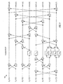
- FIG. 1 shows a flow graph of an 8-point IDCT.
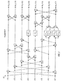
- FIG. 2 shows a flow graph of an 8-point DCT.
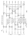
- FIG. 3 shows a flow graph of an 8-point IDCT with common factors.
- FIG. 4 shows a flow graph of an 8-point DCT with common factors.
- FIG. 5 shows a look-up table storing the numbers of operations for multiplication with different rational dyadic constant values.
- FIG. 6 shows a block diagram of a two-dimensional (2D) IDCT.
- FIG. 7 shows a block diagram of an image/video encoding and decoding system.
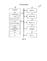
- FIG. 8 shows a block diagram of an encoding system.
- FIG. 9 shows a block diagram of a decoding system.
- the techniques described herein may be used for various types of transforms such as DCT, IDCT, discrete Fourier transform (DFT), inverse DFT (IDFT), modulated lapped transform (MLT), inverse MLT, modulated complex lapped transform (MCLT), inverse MCLT, etc.
- DFT discrete Fourier transform
- IDFT inverse DFT
- MLT modulated lapped transform
- MCLT modulated complex lapped transform
- MCLT modulated complex lapped transform
- MCLT modulated complex lapped transform
- the 1D DCT in equation (1) operates on N spatial domain values x [0] through x [N-1] and generates N transform coefficients X [0] through X [N-1].
- the 1D IDCT in equation (2) operates on N transform coefficients and generates N spatial domain values.
- Type II DCT is one type of transform and is commonly believed to be one of the most efficient transforms among several energy compacting transforms proposed for image/video compression.
- the 1D DCT may be used for a two 2D DCT, as described below.
- the 1D IDCT may be used for a 2D IDCT.
- the efficiency of the 2D DCT/IDCT is dependent on the efficiency of the 1D DCT/IDCT.
- 1D DCT and 1D IDCT may be performed on any vector size
- 2D DCT and 2D IDCT may be performed on any block size.
- 8 ⁇ 8 DCT and 8x8 IDCT are commonly used for image and video processing, where N is equal to 8.
- 8x8 DCT and 8x8 IDCT are used as standard building blocks in various image and video coding standards such as JPEG, MPEG-1, MPEG-2, MPEG-4 (P.2), H.261, H.263, etc.
- the 1D DCT and 1D IDCT may be implemented in their original forms shown in equations (1) and (2), respectively. However, substantial reduction in computational complexity may be realized by finding factorizations that result in as few multiplications and additions as possible.
- a factorization for a transform may be represented by a flow graph that indicates specific operations to be performed for that transform.
- FIG. 1 shows a flow graph 100 of an example factorization of an 8-point IDCT.
- each addition is represented by symbol " ⁇ " and each multiplication is represented by a box.
- Each addition sums or subtracts two input values and provides an output value.
- Each multiplication multiplies an input value with a transform constant shown inside the box and provides an output value.
- the factorization in FIG. 1 has six multiplications with the following constant factors:
- Flow graph 100 receives eight scaled transform coefficients A 0 ⁇ X [0] through A 7 ⁇ X [7], performs an 8-point IDCT on these coefficients, and generates eight output samples x [0] through x [7].
- Flow graph 100 includes a number of butterfly operations.
- a butterfly operation receives two input values and generates two output values, where one output value is the sum of the two input values and the other output value is the difference of the two input values.
- the butterfly operation on input values A 0 ⁇ X [0] and A 4 ⁇ X [4] generates an output value A 0 ⁇ X [0] + A 4 ⁇ X [4] for the top branch and an output value A 0 ⁇ X [0] - A 4 ⁇ X [4] for the bottom branch.
- FIG. 2 shows a flow graph 200 of an example factorization of an 8-point DCT.
- Flow graph 200 receives eight input samples x [0] through x[7], performs an 8-point DCT on these input samples, and generates eight scaled transform coefficients 8 A 0 ⁇ X [0] through 8 A 7 ⁇ X [7] .
- the scale factors A 0 through A 7 are given above.
- the factorization in FIG. 2 has six multiplications with constant factors 1/ C ⁇ /4 , 2 C 3 ⁇ /8 and 2 S 3 ⁇ /8 .
- the flow graphs for the IDCT and DCT in FIGS. 1 and 2 are similar and involve multiplications by essentially the same constant factors (with the difference in 1/2). Such similarity may be advantageous for implementation of the DCT and IDCT on an integrated circuit. In particular, the similarity may enable savings of silicon or die area to implement the butterflies and the multiplications by transform constants, which are used in both the forward and inverse transforms.
- the factorization shown in FIG. 1 results in a total of 6 multiplications and 28 additions, which are substantially fewer than the number of multiplications and additions required for direct computation of equation (2).
- the factorization shown in FIG. 2 also results in a total of 6 multiplications and 28 additions, which are substantially fewer than the number of multiplications and additions required for direct computation of equation (1).
- the factorization in FIG. 1 performs plane rotation on two intermediate variables with C 3 ⁇ /8 and S 3 ⁇ /8 .
- the factorization in FIG. 2 performs plane rotation on two intermediate variables with 2 C 3 ⁇ /8 and 2S 3 ⁇ /8 .
- a plane rotation is achieved by multiplying an intermediate variable with both sine and cosine, e.g., cos (3 ⁇ /8) and sin (3 ⁇ / 8) in FIG. 1 .
- the multiplications for plane rotation may be efficiently performed using the computation techniques described below.
- FIGS. 1 and 2 show example factorizations of an 8-point IDCT and an 8-point DCT, respectively. These factorizations are for scaled IDCT and scaled DCT, where "scaled” refers to the scaling of the transform coefficients X [0] through X [7] with known scale factors A 0 through A 7 , respectively.
- Other factorizations have also been derived by using mappings to other known fast algorithms such as a Cooley-Tukey DFT algorithm or by applying systematic factorization procedures such as decimation in time or decimation in frequency. In general, factorization reduces the number of multiplications but does not eliminate them.
- the multiplications in FIGS. 1 and 2 are with irrational constants representing the sine and cosine of different angles, which are multiples of ⁇ /8 for the 8-point DCT and IDCT.
- An irrational constant is a constant that is not a ratio of two integers.
- the multiplications with irrational constants may be more efficiently performed in fixed-point integer arithmetic when each irrational constant is approximated by a rational dyadic constant.
- a rational dyadic constant is a rational constant with a dyadic denominator and has the form c / 2 b , where b and c are integers and b > 0 .
- Multiplication of an integer variable with a rational dyadic constant may be achieved with logical and arithmetic operations, as described below.
- the number of logical and arithmetic operations is dependent on the manner in which the computation is performed as well as the value of the rational dyadic constant.
- common factors are used to reduce the total number of operations for a transform and/or to improve the precision of the transform results.
- a common factor is a constant that is applied to one or more intermediate variables in a transform.
- An intermediate variable may also be referred to as a data value, etc.
- a common factor may be absorbed with one or more transform constants and may also be accounted for by altering one or more scale factors.
- a common factor may improve the approximation of one or more (irrational) transform constants by one or more rational dyadic constants, which may then result in a fewer total number of operations and/or improved precision.
- any number of common factors may be used for a transform, and each common factor may be applied to any number of intermediate variables in the transform.
- multiple common factors are used for a transform and are applied to multiple groups of intermediate variables of different sizes.
- multiple common factors are applied to multiple groups of intermediate variables of the same size.
- FIG. 3 shows a flow graph 300 of an 8-point IDCT with common factors.
- Flow graph 300 uses the same factorization as flow graph 100 in FIG. 1 . However, flow graph 300 uses two common factors for two groups of intermediate variables.
- a first common factor F 1 is applied to a first group of two intermediate variables X 1 and X 2 , which is generated based on transform coefficients X[2] and X [6].
- the first common factor F 1 is multiplied with X 1 , is absorbed with transform constant C ⁇ /4 , and is accounted for by altering scale factors A 2 and A 6 .
- a second common factor F 2 is applied to a second group of four intermediate variables X 3 through X 6 , which is generated based on transform coefficients X [1], X [3], X [5] and X [7].
- the second common factor F 2 is multiplied with X 4 , is absorbed with transform constants C ⁇ /4 , C 3 ⁇ /8 and S 3 ⁇ /8 , and is accounted for by altering scale factors A 1, A 3 , A 5 and A 7 .
- the first common factor F 1 may be approximated with a rational dyadic constant ⁇ 1 , which may be multiplied with X 1 to obtain an approximation of the product X 1 ⁇ F 1 .
- a scaled transform factor F 1 ⁇ C ⁇ /4 may be approximated with a rational dyadic constant ⁇ 1 , which may be multiplied with X 2 to obtain an approximation of the product X 2 ⁇ F 1 ⁇ C ⁇ /4 .
- An altered scale factor A 2 / F 1 may be applied to transform coefficient X [2] .
- An altered scale factor A 6 / F 1 may be applied to transform coefficient X [6].
- the second common factor F 2 may be approximated with a rational dyadic constant ⁇ 2 , which may be multiplied with X 4 to obtain an approximation of the product X 4 ⁇ F 2 .
- a scaled transform factor F 2 ⁇ C ⁇ /4 may be approximated with a rational dyadic constant ⁇ 2 , which may be multiplied with X 3 to obtain an approximation of the product X 3 ⁇ F 2 ⁇ C ⁇ / 4 .
- a scaled transform factor F 2 ⁇ C 3 ⁇ /8 may be approximated with a rational dyadic constant ⁇ 2
- a scaled transform factor F 2 ⁇ S 3 ⁇ /8 may be approximated with a rational dyadic constant ⁇ 2
- Rational dyadic constant ⁇ 2 may be multiplied with X 5 to obtain an approximation of the product X 5 ⁇ F 2 ⁇ C 3 ⁇ /8 and also with X 6 to obtain an approximation of the product X 6 ⁇ F 2 ⁇ C 3 ⁇ /8 .
- Rational dyadic constant ⁇ 2 may be multiplied with X 5 to obtain an approximation of the product X 5 ⁇ F 2 ⁇ S 3 ⁇ /8 and also with X 6 to obtain an approximation of the product X 6 ⁇ F 2 ⁇ S 3 ⁇ /8 .
- Altered scale factors A 1 / F 2 , A 3 / F 2 , A 5 l F 2 and A 7 / F 2 may be applied to transform coefficients X [1], X [3], X [5] and X [7], respectively.
- Six rational dyadic constants ⁇ 1 , ⁇ 1 , ⁇ 2 , ⁇ 2 , ⁇ 2 and ⁇ 2 may be defined for six constants, as follows: ⁇ 1 ⁇ F 1 , ⁇ 1 ⁇ F 1 ⁇ cos ⁇ / 4 , ⁇ 2 ⁇ F 2 , ⁇ 2 ⁇ F 2 ⁇ cos ⁇ / 4 , ⁇ 2 ⁇ F 2 ⁇ cos 3 ⁇ ⁇ / 8 , and ⁇ 2 ⁇ F 2 ⁇ sin 3 ⁇ ⁇ / 8 .
- FIG. 4 shows a flow graph 400 of an 8-point DCT with common factors.
- Flow graph 400 uses the same factorization as flow graph 200 in FIG. 2 . However, flow graph 400 uses two common factors for two groups of intermediate variables.
- a first common factor F a is applied to a first group of two intermediate variables X a and X b , which is used to generate transform coefficients X [2] and X [6].
- the first common factor F a is multiplied with X a , is absorbed with transform constant 1/ C ⁇ /4 , and is accounted for by altering scale factors A 2 and A 6 .
- a second common factor F b is applied to a second group of four intermediate variables X c through X f , which is used to generate transform coefficients X [1], X [3], X [5] and X [7].
- the second common factor F b is multiplied with X d , is absorbed with transform constants 1/ C ⁇ /4 , 2 C 3 ⁇ /8 and 2 S 3 ⁇ /8 , and is accounted for by altering scale factors A 1 , A 3 , A 5 and A 7 .
- the first common factor F a may be approximated with a rational dyadic constant ⁇ a , which may be multiplied with X a to obtain an approximation of the product X a ⁇ F a .
- a scaled transform factor F a / C ⁇ /4 may be approximated with a rational dyadic constant ⁇ a, which may be multiplied with X b to obtain an approximation of the product X b ⁇ F a / C ⁇ /4 .
- Altered scale factors A 2 / F a and A 6 / F a may be applied to transform coefficients X [2] and X [6], respectively.
- the second common factor F b may be approximated with a rational dyadic constant ⁇ b , which may be multiplied with X d to obtain an approximation of the product X d ⁇ F b .
- a scaled transform factor F b / C ⁇ /4 may be approximated with a rational dyadic constant ⁇ b , which may be multiplied with X c to obtain an approximation of the product X c ⁇ F b / C ⁇ /4 .
- a scaled transform factor 2 F b ⁇ C 3 ⁇ /8 may be approximated with a rational dyadic constant ⁇ b
- a scaled transform factor 2 F b ⁇ S 3 ⁇ /8 may be approximated with a rational dyadic constant ( ⁇ b .
- Rational dyadic constant ⁇ b may be multiplied with X e to obtain an approximation of the product 2 X e ⁇ F b ⁇ C 3 ⁇ /8 and also with X f to obtain an approximation of the product 2 X f ⁇ F b ⁇ C 3 ⁇ /8 .
- Rational dyadic constant ⁇ b may be multiplied with X e to obtain an approximation of the product 2 X e ⁇ F b ⁇ S 3 ⁇ /8 and also with X f to obtain an approximation of the product 2 X f ⁇ F b ⁇ S 3 ⁇ /8 .
- Altered scale factors A 1 / F b , A 3 / F b , A 5 l F b and A 7 / F b may be applied to transform coefficients X [1], X [3], X [5] and X[7], respectively.
- Six rational dyadic constants ⁇ a , ⁇ a , ⁇ b , ⁇ b , ⁇ b and ⁇ b may be defined for six constants, as follows: ⁇ a ⁇ F a , ⁇ a ⁇ F a / cos ⁇ / 4 , ⁇ b ⁇ F b , ⁇ b ⁇ F b / cos ⁇ / 4 , ⁇ b ⁇ 2 ⁇ F b ⁇ cos 3 ⁇ ⁇ / 8 , and ⁇ b ⁇ 2 ⁇ F b ⁇ sin 3 ⁇ ⁇ / 8 .
- FIGS. 3 and 4 show example use of common factors for specific factorizations of 8-point IDCT and 8-point DCT, respectively.
- Common factors may be used for other factorizations of the DCT and IDCT and also for other types of transforms.
- a common factor may be applied to a group of at least one intermediate variable in a transform. This group of intermediate variable(s) may be generated from a group of input values (e.g., as shown in FIG. 3 ) or used to generate a group of output values (e.g., as shown in FIG. 4 ).
- the common factor may be accounted for by the scale factors applied to the input values or the output values.
- Multiple common factors may be applied to multiple groups of intermediate variables, and each group may include any number of intermediate variables.
- the selection of the groups may be dependent on various factors such as the factorization of the transform, where the transform constants are located within the transform, etc.
- Multiple common factors may be applied to multiple groups of intermediate variables of the same size (not shown in FIGS. 3 and 4 ) or different sizes (as shown in FIGS. 3 and 4 ). For example, three common factors may be used for the factorization shown in FIG.
- Multiplication of an intermediate variable x with a rational dyadic constant u may be performed in various manners in fixed-point integer arithmetic.
- the multiplication may be performed using logical operations (e.g., left shift, right shift, bit-inversion, etc.), arithmetic operations (e.g., add, subtract, sign-inversion, etc.) and/or other operations.
- the number of logical and arithmetic operations needed for the multiplication of x with u is dependent on the manner in which the computation is performed and the value of the rational dyadic constant u .
- Different computation techniques may require different numbers of logical and arithmetic operations for the same multiplication of x with u .
- a given computation technique may require different numbers of logical and arithmetic operations for the multiplication of x with different values of u .
- a common factor may be selected for a group of intermediate variables based on criteria such as:
- arithmetic operations may be more complex than logical operations, so reducing the number of arithmetic operations may be more important.
- computational complexity may be quantified based solely on the number of arithmetic operations, without taking into account logical operations.
- logical operations e.g., shifts
- reducing the number of logical operations e.g., reducing the number of shift operations and/or the total number of bits shifted
- a weighted average number of logical and arithmetic operations may be used, where the weights may represent the relative complexities of the logical and arithmetic operations.
- the precision of the results may be quantified based on various metrics such as those given in Table 6 below. In general, it is desirable to reduce the number of logical and arithmetic operations (or computational complexity) for a given precision. It may also be desirable to trade off complexity for precision, e.g., to achieve higher precision at the expense of some additional operations.
- multiplication may be performed on a group of intermediate variables with a group of rational dyadic constants that approximates a group of at least one irrational constant (for at least one transform factor) scaled by that common factor.
- Multiplication in fixed-point integer arithmetic may be performed in various manners. For clarity, computation techniques that perform multiplication with shift and add operations and using intermediate results are described below. These computation techniques may reduce the total number of shift and add operations for the DCT and IDCT.
- Multiplication of an integer variable x with an irrational constant ⁇ in fixed-point integer arithmetic may be achieved by approximating the irrational constant with a rational dyadic constant, as follows: ⁇ ⁇ c / 2 b , where ⁇ is the irrational constant to be approximated, c /2 b is the rational dyadic constant, b and c are integers, and b > 0.
- y i may be equal to y j + y k ⁇ 2 s i , y j - y k ⁇ 2 s i , or - y j + y k ⁇ 2 s i .
- Each intermediate value y i in the series may be derived based on two prior intermediate values y j and y k in the series, where either y j or y k may be equal to zero.
- the total number of additions and shifts for the multiplication is determined by the number of intermediate values in the series, which is t , as well as the expression used for each intermediate value.
- the multiplication by rational dyadic constant u is essentially unrolled into a series of shift and add operations.
- the series is defined such that the final value in the series becomes the desired integer-valued product, or y t ⁇ y .
- the multiplication of integer variable x with irrational constant ⁇ may be approximated with a series of intermediate values generated by shift and add operations and using intermediate results (or prior generated intermediate values) to reduce the total number of operations.
- Multiplication of an integer variable x with two irrational constants ⁇ and ⁇ in fixed-point integer arithmetic may be achieved by approximating the irrational constants with rational dyadic constants, as follows: ⁇ ⁇ c / 2 b and ⁇ ⁇ e / 2 d , where c /2 b and e /2 d are two rational dyadic constants, b, c , d and e are integers, b > 0 and d > 0.
- the series is defined such that the desired integer-valued products are obtained at steps m and n , as follows: w m ⁇ y and w n ⁇ z , where m,n ⁇ t and either m or n is equal to t.
- the multiplication of integer variable x with irrational constants ⁇ and ⁇ may be approximated with a common series of intermediate values generated by shift and add operations and using intermediate results to reduce the total number of operations.
- Equation (15) the expression to the left of " ⁇ ” involves an addition or subtraction of zero (denoted by y 0 ) and may be performed with one shift, as shown by the expression to the right of " ⁇ ".
- equation (16) the expression to the left of " ⁇ ” involves a shift by zero bits (denoted by 2o) and may be performed with one addition, as shown by the expression to the right of " ⁇ ”. Equations (15) and (16) may be applied to equation (8) in the computation of y i as well as to equation (13) in the computation of w i .
- FIGS. 1 through 4 may be efficiently performed using the computation techniques described above.
- the binary value to the right of "//" is an intermediate constant that is multiplied with variable x.
- the multiplication in equation (18) may be performed with three additions and three shifts to generate three intermediate values y 2 , y 3 and y 4 .
- the two multiplications in equation (22) may be jointly performed with five additions and five shifts to generate seven intermediate values w 2 through w 8 . Additions of zeros are omitted in the generation of w 3 and w 6 . Shifts by zero are omitted in the generation of w 4 and w 5 .
- any desired precision may be achieved by using sufficient number of bits for the approximation of each transform constant.
- irrational constants 1/ C ⁇ /4 , C 3 ⁇ /8 and S 3 ⁇ /8 may be approximated with rational dyadic constants. Multiplications with the rational dyadic constants may be achieved using the computation techniques described above.
- different values of common factors F 1 and F 2 may result in different total numbers of logical and arithmetic operations for the IDCT and different levels of precision for the output samples x [0] through x[7]. Different combinations of values for F 1 and F 2 may be evaluated. For each combination of values, the total number of logical and arithmetic operations for the IDCT and the precision of the output samples may be determined.
- rational dyadic constants ⁇ 1 and ⁇ 1 may be obtained for F 1 and F 1 ⁇ C ⁇ / 4 , respectively.
- the numbers of logical and arithmetic operations may then be determined for multiplication of X 1 with ⁇ 1 and multiplication of X 2 with ⁇ 1 .
- rational dyadic constants ⁇ 2 , ⁇ 2, ⁇ 2 and ⁇ 2 may be obtained for F 2 , F 2 ⁇ C ⁇ /4 , F 2 ⁇ C 3 ⁇ /8 and F 2 ⁇ S 3 ⁇ /8 , respectively.
- the numbers of logical and arithmetic operations may then be determined for multiplication of X 4 with ⁇ 2 , multiplication of X 3 with ⁇ 2 , and multiplications of X 5 with both ⁇ 2 and ⁇ 2 .
- the number of operations for multiplications of X 6 with ⁇ 2 and ⁇ 2 is equal to the number of operations for multiplications of X 5 with ⁇ 2 and ⁇ 2 .
- the number of logical and arithmetic operations may be pre-computed for multiplication with different possible values of rational dyadic constants.
- the pre-computed numbers of logical and arithmetic operations may be stored in a look-up table or some other data structure.
- FIG. 5 shows a look-up table 500 that stores the numbers of logical and arithmetic operations for multiplication with different rational dyadic constant values.
- Look-up table 500 is a two-dimensional table with different possible values of a first rational dyadic constant C 1 on the horizontal axis and different possible values of a second rational dyadic constant C 2 on the vertical axis.
- the number of possible values for each rational dyadic constant is dependent on the number of bits used for that constant. For example, if C 1 is represented with 13 bits, then there are 8192 possible values for C 1 .
- the entry in the i -th column and j-th row of look-up table 500 contains the number of logical and arithmetic operations for joint multiplication of intermediate variable x with both c i for the first rational dyadic constant C 1 and c j for the second rational dyadic constant C 2 .
- the value for each entry in look-up table 500 may be determined by evaluating different possible series of intermediate values for the joint multiplication with c i and c j for that entry and selecting the best series, e.g., the series with the fewest operations.
- rational dyadic constants ⁇ 1 and ⁇ 1 may be determined.
- the numbers of logical and arithmetic operations for multiplication of X 1 with ⁇ 1 and multiplication of X 2 with ⁇ 1 may be readily determined from the entries in the first row of look-up table 500, where ⁇ 1 and ⁇ 1 correspond to C 1 .
- rational dyadic constants ⁇ 2 , ⁇ 2 , ⁇ 2 and ⁇ 2 may be determined.
- the numbers of logical and arithmetic operations for multiplication of X 4 with ⁇ 2 and multiplication of X 3 with ⁇ 2 may be determined from the entries in the first row of look-up table 500, where ⁇ 2 and ⁇ 2 correspond to C 1 .
- the number of logical and arithmetic operations for joint multiplication of X 5 with ⁇ 2 and ⁇ 2 may be determined from an appropriate entry in look-up table 500, where ⁇ 2 may correspond to C 1 and ⁇ 2 may correspond to C 2 , or vice versa.
- the precision metrics in Table 6 may be determined for a sufficient number of iterations with different random input data.
- the values of F 1 and F 2 that result in poor precision (e.g., failure of the metrics) may be discarded, and the values of F 1 and F 2 that result in good precision (e.g., pass of the metrics) may be retained.
- Tables 1 through 5 show five fixed-point approximations for the IDCT in FIG. 3 , which are denoted as algorithms A, B, C, D and E. These approximations are for two groups of factors, with one group including ⁇ 1 and ⁇ 1 and another group including ⁇ 2 , ⁇ 2, ⁇ 2 and ⁇ 2 .
- the common factor for each group is given in the first column.
- the common factors improve the precision of the rational dyadic constant approximations and may be merged with the appropriate scale factors in the flow graph for the IDCT.
- the original values (which may be 1 or irrational constants) are given in the third column.
- the rational dyadic constant for each original value scaled by its common factor is given in the fourth column.
- the series of intermediate values for the multiplication of intermediate variable x with one or two rational dyadic constants is given in the fifth column.
- the numbers of add and shift operations for each multiplication are given in the sixth and seventh columns, respectively.
- the total number of add operations for the IDCT is equal to the sum of all add operations in the sixth column plus the last entry again (to account for multiplication of each of X 5 and X 6 with both ⁇ 2 and ⁇ 2 ) plus 28 add operations for all of the butterflies in the flow graph.
- the total number of shift operations for the IDCT is equal to the sum of all shift operations in the last column plus the last entry again.
- Table 1 gives the details of algorithm A, which uses a common factor of 1/1.0000442471 for each of the two groups.
- Table 2 gives the details of algorithm B, which uses a common factor of 1/1.0000442471 for the first group and a common factor of 1/1.02053722659 for the second group.
- Table 3 gives the details of algorithm C, which uses a common factor of 1/0.87734890555 for the first group and a common factor of 1/1.02053722659 for the second group.
- Table 4 gives the details of algorithm D, which uses a common factor of 1/0.87734890555 for the first group and a common factor of 1/0.89062054308 for the second group.
- Table 5 gives the details of algorithm E, which uses a common factor of 1/0.87734890555 for the first group and a common factor of 1/1.22387468002 for the second group.
- the precision of the output samples from an approximate IDCT may be quantified based on metrics defined in IEEE Standard 1180-1190 and its pending replacement.
- This standard specifies testing a reference 64-bit floating-point DCT followed by the approximate IDCT using data from a random number generator.
- the reference DCT receives random data for a block of input pixels and generates transform coefficients.
- the approximate IDCT receives the transform coefficients (appropriately rounded) and generates a block of reconstructed pixels.
- the reconstructed pixels are compared against the input pixels using five metrics, which are given in Table 6. Additionally, the approximate IDCT is required to produce all zeros when supplied with zero transform coefficients and to demonstrate near-DC inversion behavior. All five algorithms A through E given above pass all of the metrics in Table 6.
- the 1D IDCT shown in FIG. 3 may be used for a 2D IDCT.
- the 1D DCT shown in FIG. 4 may be used for a 2D DCT.
- FIG. 6 shows a design of a 2D IDCT 600 implemented in a scaled and separable fashion.
- 2D IDCT 600 comprises an input scaling stage 612, followed by a first scaled 1D IDCT stage 614 for the columns (or rows), further followed by a second scaled 1D IDCT stage 616 for the rows (or columns), and concluding with an output scaling stage 618.
- S P + R bits may be used in the conversion of the scale factors to integers, and right shifts by R bits may be performed after multiplications.
- S may be any suitable value that can facilitate implementations on hardware platforms, e.g., S may be 15 or 16 for platforms with signed/unsigned 16-bit multipliers.
- First 1D IDCT stage 614 performs an 8-point IDCT on each column of the block of scaled transform coefficients.
- Second 1D IDCT stage 616 performs an 8-point IDCT on each row of an intermediate block generated by first 1D IDCT stage 614.
- the 1D IDCTs for the first and second stages may operate directly on their input data without doing any internal pre- or post scaling.
- output scaling stage 618 may shift the resulting quantities from second 1D IDCT stage 616 by P bits to the right to generate the output samples for the 2D IDCT.
- the scale factors and the precision constant P may be chosen such that the entire 2D IDCT may be implemented using registers of the desired width.
- the 2D DCT may be performed in similar manner as the 2D IDCT.
- the 2D DCT may be performed by (a) pre-multiplying a block of spatial domain samples, (b) performing 1D DCT on each column (or row) of the block of scaled samples to generate an intermediate block, (c) performing 1D DCT on each row (or column) of the intermediate block, and (d) scaling the output of the second 1D DCT stage to generate a block of transform coefficients for the 2D DCT.
- the techniques described herein may be used for any type of transform such as DCT, IDCT, DFT, IDFT, MLT, inverse MLT, MCLT, inverse MCLT, etc.
- the techniques may also be used for any factorization of a transform, with several example factorizations being given in FIGS. 1 through 4 .
- the groups for the common factors may be selected based on the factorization, as described above.
- the techniques may also be used for transforms of any size, with example 8-point transforms being given in FIGS. 1 through 4 .
- the techniques may also be used in conjunction with any common factor selection criteria such as total number of logical and arithmetic operations, total number of arithmetic operations, precision of the results, etc.
- the number of operations for a transform may be dependent on the manner in which multiplications are performed.
- the computation techniques described above unroll multiplications into series of shift and add operations, use intermediate results to reduce the number of operations, and perform joint multiplication with multiple constants using a common series.
- the multiplications may also be performed with other computation techniques, which may influence the selection of the common factors.
- Transforms with common factors may be used for various applications such as image and video processing, communication, computing, data networking, data storage, graphics, etc.
- Example use of transforms for video processing is described below.
- FIG. 7 shows a block diagram of an image/video encoding and decoding system 700.
- a DCT unit 720 receives an input data block and generates a transform coefficient block.
- the input data block may be an N ⁇ N block of pixels, an N ⁇ N block of pixel difference values (or residue), or some other type of data generated from a source signal, e.g., a video signal.
- the pixel difference values may be differences between two blocks of pixels, differences between a block of pixels and a block of predicted pixels, etc. N may be equal to 8 or some other value.
- An encoder 730 receives the transform coefficient block from DCT unit 720, encodes the transform coefficients, and generates compressed data.
- the compressed data may be stored in a storage unit and/or sent via a communication channel (cloud 740).
- a decoder 760 receives the compressed data from storage unit or communication channel 740 and reconstructs the transform coefficients.
- An IDCT unit 770 receives the reconstructed transform coefficients and generates an output data block.
- the output data block may be an N ⁇ N block of reconstructed pixels, an N ⁇ N block of reconstructed pixel difference values, etc.
- the output data block may be an estimate of the input data block provided to DCT unit 720 and may be used to reconstruct the source signal.
- FIG. 8 shows a block diagram of an encoding system 800, which may be used for encoding system 710 in FIG. 7 .
- a capture device/memory 810 may receive a source signal, perform conversion to digital format, and provides input/raw data. Capture device 810 may be a video camera, a digitizer, or some other device.
- a processor 820 processes the raw data and generates compressed data. Within processor 820, the raw data may be transformed by a DCT unit 822, scanned by a zig-zag scan unit 824, quantized by a quantizer 826, encoded by an entropy encoder 828, and packetized by a packetizer 830.
- DCT unit 822 may perform 2D DCTs on the raw data in accordance with the teclmiques described above.
- Each of units 822 through 830 may be implemented a hardware, firmware and/or software.
- DCT unit 822 may be implemented with dedicated hardware, a set of instructions for an arithmetic logic unit (ALU), etc.
- ALU arithmetic logic unit
- a storage unit 840 may store the compressed data from processor 820.
- a transmitter 842 may transmit the compressed data.
- a controller/processor 850 controls the operation of various units in encoding system 800.
- a memory 852 stores data and program codes for encoding system 800.
- One or more buses 860 interconnect various units in encoding system 800.
- FIG. 9 shows a block diagram of a decoding system 900, which may be used for decoding system 750 in FIG. 7 .
- a receiver 910 may receive compressed data from an encoding system, and a storage unit 912 may store the received compressed data.
- a processor 920 processes the compressed data and generates output data.
- the compressed data may be de-packetized by a de-packetizer 922, decoded by an entropy decoder 924, inverse quantized by an inverse quantizer 926, placed in the proper order by an inverse zig-zag scan unit 928, and transformed by an IDCT unit 930.
- IDCT unit 930 may perform 2D IDCTs on the reconstructed transform coefficients in accordance with the techniques described above.
- Each of units 922 through 930 may be implemented a hardware, firmware and/or software.
- IDCT unit 930 may be implemented with dedicated hardware, a set of instructions for an ALU, etc.
- a display unit 940 displays reconstructed images and video from processor 920.
- a controller/processor 950 controls the operation of various units in decoding system 900.
- a memory 952 stores data and program codes for decoding system 900.
- One or more buses 960 interconnect various units in decoding system 900.
- Processors 820 and 920 may each be implemented with one or more application specific integrated circuits (ASICs), digital signal processors (DSPs), and/or some other type of processors. Alternatively, processors 820 and 920 may each be replaced with one or more random access memories (RAMs), read only memory (ROMs), electrical programmable ROMs (EPROMs), electrically erasable programmable ROMs (EEPROMs), magnetic disks, optical disks, and/or other types of volatile and nonvolatile memories known in the art.
- ASICs application specific integrated circuits
- DSPs digital signal processors
- RAMs random access memories
- ROMs read only memory
- EPROMs electrical programmable ROMs
- EEPROMs electrically erasable programmable ROMs
- magnetic disks magnetic disks
- optical disks and/or other types of volatile and nonvolatile memories known in the art.
- the techniques described herein may be implemented in hardware, firmware, software, or a combination thereof.
- the logical (e.g., shift) and arithmetic (e.g., add) operations for multiplication of a data value with a constant value may be implemented with one or more logics, which may also be referred to as units, modules, etc.
- a logic may be hardware logic comprising logic gates, transistors, and/or other circuits known in the art.
- a logic may also be firmware and/or software logic comprising machine-readable codes.
- an apparatus comprises a first logic to perform multiplication of a first group of at least one data value with a first group of at least one rational dyadic constant that approximates a first group of at least one irrational constant scaled by a first common factor.
- the apparatus further comprises a second logic to perform multiplication of a second group of at least one data value with a second group of at least one rational dyadic constant that approximates a second group of at least one irrational constant scaled by a second common factor.
- the first and second groups of at least one data value have different sizes.
- the first and second logic may be separate logics, the same common logic, or shared logic.
- multiplication of a data value with a constant value may be achieved with machine-readable codes that perform the desired logical and arithmetic operations.
- the codes may be hardwired or stored in a memory (e.g., memory 852 in FIG. 8 or 952 in FIG. 9 ) and executed by a processor (e.g., processor 850 or 950) or some other hardware unit.
- the techniques described herein may be implemented in various types of apparatus.
- the techniques may be implemented in different types of processors, different types of integrated circuits, different types of electronics devices, different types of electronics circuits, etc.
- a general-purpose processor may be a microprocessor, but in the alternative, the processor may be any conventional processor, controller, microcontroller, or state machine.
- a processor may also be implemented as a combination of computing devices, e.g., a combination of a DSP and a microprocessor, a plurality of microprocessors, one or more microprocessors in conjunction with a DSP core, or any other such configuration.
- the functions described may be implemented in hardware, software, firmware, or any combination thereof. If implemented in software, the functions may be stored on or transmitted over as one or more instructions or code on a computer-readable medium.
- Computer-readable media includes both computer storage media and communication media including any medium that facilitates transfer of a computer program from one place to another.
- a storage media may be any available media that can be accessed by a computer.
- such computer-readable media can comprise RAM, ROM, EEPROM, CD-ROM or other optical disk storage, magnetic disk storage or other magnetic storage devices, or any other medium that can be used to carry or store desired program code in the form of instructions or data structures and that can be accessed by a computer.
- any connection is properly termed a computer-readable medium.
- the software is transmitted from a website, server, or other remote source using a coaxial cable, fiber optic cable, twisted pair, digital subscriber line (DSL), or wireless technologies such as infrared, radio, and microwave
- the coaxial cable, fiber optic cable, twisted pair, DSL, or wireless technologies such as infrared, radio, and microwave are included in the definition of medium.
- Disk and disc includes compact disc (CD), laser disc, optical disc, digital versatile disc (DVD), floppy disk and blu-ray disc where disks usually reproduce data magnetically, while discs reproduce data optically with lasers. Combinations of the above should also be included within the scope of computer-readable media.
Landscapes
- Engineering & Computer Science (AREA)
- Physics & Mathematics (AREA)
- General Physics & Mathematics (AREA)
- Theoretical Computer Science (AREA)
- Mathematical Analysis (AREA)
- Mathematical Optimization (AREA)
- Pure & Applied Mathematics (AREA)
- Computational Mathematics (AREA)
- Mathematical Physics (AREA)
- Computing Systems (AREA)
- General Engineering & Computer Science (AREA)
- Data Mining & Analysis (AREA)
- Discrete Mathematics (AREA)
- Signal Processing (AREA)
- Multimedia (AREA)
- Algebra (AREA)
- Databases & Information Systems (AREA)
- Software Systems (AREA)
- Nonlinear Science (AREA)
- Complex Calculations (AREA)
- Compression Or Coding Systems Of Tv Signals (AREA)
Applications Claiming Priority (3)
| Application Number | Priority Date | Filing Date | Title |
|---|---|---|---|
| US75846406P | 2006-01-11 | 2006-01-11 | |
| US11/621,945 US8595281B2 (en) | 2006-01-11 | 2007-01-10 | Transforms with common factors |
| EP07710066A EP1999641A2 (de) | 2006-01-11 | 2007-01-11 | Transformationen mit verminderter komplexität und/oder verbesserter präzision mittels gemeinsamer faktoren |
Related Parent Applications (2)
| Application Number | Title | Priority Date | Filing Date |
|---|---|---|---|
| EP07710066.7 Division | 2007-01-11 | ||
| EP07710066A Division EP1999641A2 (de) | 2006-01-11 | 2007-01-11 | Transformationen mit verminderter komplexität und/oder verbesserter präzision mittels gemeinsamer faktoren |
Publications (2)
| Publication Number | Publication Date |
|---|---|
| EP2477121A2 true EP2477121A2 (de) | 2012-07-18 |
| EP2477121A3 EP2477121A3 (de) | 2015-01-21 |
Family
ID=38257126
Family Applications (2)
| Application Number | Title | Priority Date | Filing Date |
|---|---|---|---|
| EP12161794.8A Withdrawn EP2477121A3 (de) | 2006-01-11 | 2007-01-11 | Transformationen mit gemeinsamen Faktoren |
| EP07710066A Withdrawn EP1999641A2 (de) | 2006-01-11 | 2007-01-11 | Transformationen mit verminderter komplexität und/oder verbesserter präzision mittels gemeinsamer faktoren |
Family Applications After (1)
| Application Number | Title | Priority Date | Filing Date |
|---|---|---|---|
| EP07710066A Withdrawn EP1999641A2 (de) | 2006-01-11 | 2007-01-11 | Transformationen mit verminderter komplexität und/oder verbesserter präzision mittels gemeinsamer faktoren |
Country Status (15)
| Country | Link |
|---|---|
| US (1) | US8595281B2 (de) |
| EP (2) | EP2477121A3 (de) |
| JP (1) | JP5086274B2 (de) |
| KR (1) | KR101028676B1 (de) |
| CN (2) | CN101375274B (de) |
| AU (1) | AU2007204645B2 (de) |
| BR (1) | BRPI0706474A2 (de) |
| CA (1) | CA2633897C (de) |
| IL (1) | IL192075A0 (de) |
| MX (1) | MX2008008987A (de) |
| NO (1) | NO20083465L (de) |
| NZ (1) | NZ568993A (de) |
| RU (1) | RU2429531C2 (de) |
| TW (1) | TWI359364B (de) |
| WO (1) | WO2007082272A2 (de) |
Families Citing this family (16)
| Publication number | Priority date | Publication date | Assignee | Title |
|---|---|---|---|---|
| US20070200738A1 (en) * | 2005-10-12 | 2007-08-30 | Yuriy Reznik | Efficient multiplication-free computation for signal and data processing |
| US8595281B2 (en) * | 2006-01-11 | 2013-11-26 | Qualcomm Incorporated | Transforms with common factors |
| US20070271321A1 (en) * | 2006-01-11 | 2007-11-22 | Qualcomm, Inc. | Transforms with reduce complexity and/or improve precision by means of common factors |
| US8849884B2 (en) | 2006-03-29 | 2014-09-30 | Qualcom Incorporate | Transform design with scaled and non-scaled interfaces |
| US8654833B2 (en) * | 2007-09-26 | 2014-02-18 | Qualcomm Incorporated | Efficient transformation techniques for video coding |
| US8248660B2 (en) * | 2007-12-14 | 2012-08-21 | Qualcomm Incorporated | Efficient diffusion dithering using dyadic rationals |
| US9110849B2 (en) * | 2009-04-15 | 2015-08-18 | Qualcomm Incorporated | Computing even-sized discrete cosine transforms |
| US8762441B2 (en) * | 2009-06-05 | 2014-06-24 | Qualcomm Incorporated | 4X4 transform for media coding |
| US9069713B2 (en) * | 2009-06-05 | 2015-06-30 | Qualcomm Incorporated | 4X4 transform for media coding |
| US9081733B2 (en) * | 2009-06-24 | 2015-07-14 | Qualcomm Incorporated | 16-point transform for media data coding |
| US8451904B2 (en) | 2009-06-24 | 2013-05-28 | Qualcomm Incorporated | 8-point transform for media data coding |
| US9118898B2 (en) | 2009-06-24 | 2015-08-25 | Qualcomm Incorporated | 8-point transform for media data coding |
| US9075757B2 (en) | 2009-06-24 | 2015-07-07 | Qualcomm Incorporated | 16-point transform for media data coding |
| US9185422B2 (en) * | 2010-07-15 | 2015-11-10 | Qualcomm Incorporated | Variable localized bit-depth increase for fixed-point transforms in video coding |
| US9824066B2 (en) | 2011-01-10 | 2017-11-21 | Qualcomm Incorporated | 32-point transform for media data coding |
| US11030777B2 (en) * | 2018-09-14 | 2021-06-08 | Sony Group Corporation | Adaptive subband coding for lifting transform |
Family Cites Families (43)
| Publication number | Priority date | Publication date | Assignee | Title |
|---|---|---|---|---|
| US4864529A (en) * | 1986-10-09 | 1989-09-05 | North American Philips Corporation | Fast multiplier architecture |
| JPH01175186A (ja) | 1987-12-29 | 1989-07-11 | Nitto Denko Corp | 熱接着用プレス装置における熱加圧具 |
| JP2711176B2 (ja) | 1990-10-02 | 1998-02-10 | アロカ株式会社 | 超音波画像処理装置 |
| CA2060407C (en) | 1991-03-22 | 1998-10-27 | Jack M. Sacks | Minimum difference processor |
| US5233551A (en) * | 1991-10-21 | 1993-08-03 | Rockwell International Corporation | Radix-12 DFT/FFT building block |
| US5285402A (en) * | 1991-11-22 | 1994-02-08 | Intel Corporation | Multiplyless discrete cosine transform |
| US5539836A (en) * | 1991-12-20 | 1996-07-23 | Alaris Inc. | Method and apparatus for the realization of two-dimensional discrete cosine transform for an 8*8 image fragment |
| TW284869B (de) * | 1994-05-27 | 1996-09-01 | Hitachi Ltd | |
| US5712809A (en) | 1994-10-31 | 1998-01-27 | Vivo Software, Inc. | Method and apparatus for performing fast reduced coefficient discrete cosine transforms |
| US5701263A (en) * | 1995-08-28 | 1997-12-23 | Hyundai Electronics America | Inverse discrete cosine transform processor for VLSI implementation |
| US5930160A (en) * | 1996-06-22 | 1999-07-27 | Texas Instruments Incorporated | Multiply accumulate unit for processing a signal and method of operation |
| JP3263807B2 (ja) | 1996-09-09 | 2002-03-11 | ソニー株式会社 | 画像符号化装置および画像符号化方法 |
| US6058215A (en) | 1997-04-30 | 2000-05-02 | Ricoh Company, Ltd. | Reversible DCT for lossless-lossy compression |
| JP3957829B2 (ja) * | 1997-08-29 | 2007-08-15 | 株式会社オフィスノア | 動画像情報の圧縮方法およびそのシステム |
| KR100270799B1 (ko) * | 1998-01-30 | 2000-11-01 | 김영환 | 이산코사인변환/역이산코사인변환 프로세서 |
| US6189021B1 (en) | 1998-09-15 | 2001-02-13 | Winbond Electronics Corp. | Method for forming two-dimensional discrete cosine transform and its inverse involving a reduced number of multiplication operations |
| US6757326B1 (en) * | 1998-12-28 | 2004-06-29 | Motorola, Inc. | Method and apparatus for implementing wavelet filters in a digital system |
| US6473534B1 (en) * | 1999-01-06 | 2002-10-29 | Hewlett-Packard Company | Multiplier-free implementation of DCT used in image and video processing and compression |
| WO2000055757A1 (en) | 1999-03-17 | 2000-09-21 | The Johns Hopkins University | A fast multiplierless transform |
| US6529634B1 (en) | 1999-11-08 | 2003-03-04 | Qualcomm, Inc. | Contrast sensitive variance based adaptive block size DCT image compression |
| US6760486B1 (en) | 2000-03-28 | 2004-07-06 | General Electric Company | Flash artifact suppression in two-dimensional ultrasound imaging |
| AU2001268309A1 (en) * | 2000-06-09 | 2001-12-17 | Walter E Pelton | Methods for reducing the number of computations in a discrete fourier transform |
| JP4266512B2 (ja) | 2000-12-27 | 2009-05-20 | キヤノン株式会社 | データ処理装置 |
| US7007054B1 (en) * | 2000-10-23 | 2006-02-28 | International Business Machines Corporation | Faster discrete cosine transforms using scaled terms |
| US6766341B1 (en) * | 2000-10-23 | 2004-07-20 | International Business Machines Corporation | Faster transforms using scaled terms |
| ATE375571T1 (de) * | 2001-06-12 | 2007-10-15 | Silicon Optix Inc | Verfahen und vorrichtung zur verarbeitung einer nichtlinearen zweidimensionalen räumlichen transformation |
| US6870963B2 (en) | 2001-06-15 | 2005-03-22 | Qualcomm, Inc. | Configurable pattern optimizer |
| US7082450B2 (en) | 2001-08-30 | 2006-07-25 | Nokia Corporation | Implementation of a transform and of a subsequent quantization |
| US20030074383A1 (en) * | 2001-10-15 | 2003-04-17 | Murphy Charles Douglas | Shared multiplication in signal processing transforms |
| US6917955B1 (en) * | 2002-04-25 | 2005-07-12 | Analog Devices, Inc. | FFT processor suited for a DMT engine for multichannel CO ADSL application |
| US7395210B2 (en) * | 2002-11-21 | 2008-07-01 | Microsoft Corporation | Progressive to lossless embedded audio coder (PLEAC) with multiple factorization reversible transform |
| US7792891B2 (en) * | 2002-12-11 | 2010-09-07 | Nvidia Corporation | Forward discrete cosine transform engine |
| TWI220716B (en) * | 2003-05-19 | 2004-09-01 | Ind Tech Res Inst | Method and apparatus of constructing a hardware architecture for transfer functions |
| RU2305377C2 (ru) | 2003-05-20 | 2007-08-27 | Корпорация "САМСУНГ ЭЛЕКТРОНИКС Ко., Лтд." | Способ уменьшения искажения сжатого видеоизображения и устройство для его реализации |
| US7487193B2 (en) * | 2004-05-14 | 2009-02-03 | Microsoft Corporation | Fast video codec transform implementations |
| US7587093B2 (en) * | 2004-07-07 | 2009-09-08 | Mediatek Inc. | Method and apparatus for implementing DCT/IDCT based video/image processing |
| US7489826B2 (en) * | 2004-10-07 | 2009-02-10 | Infoprint Solutions Company, Llc | Compensating for errors in performance sensitive transformations |
| US7421139B2 (en) * | 2004-10-07 | 2008-09-02 | Infoprint Solutions Company, Llc | Reducing errors in performance sensitive transformations |
| CN100388316C (zh) * | 2005-04-19 | 2008-05-14 | 展讯通信(上海)有限公司 | 高精度的无乘法器的数字余弦变换电路及其变换方法 |
| US20070200738A1 (en) * | 2005-10-12 | 2007-08-30 | Yuriy Reznik | Efficient multiplication-free computation for signal and data processing |
| US20070271321A1 (en) * | 2006-01-11 | 2007-11-22 | Qualcomm, Inc. | Transforms with reduce complexity and/or improve precision by means of common factors |
| US8595281B2 (en) * | 2006-01-11 | 2013-11-26 | Qualcomm Incorporated | Transforms with common factors |
| US8849884B2 (en) * | 2006-03-29 | 2014-09-30 | Qualcom Incorporate | Transform design with scaled and non-scaled interfaces |
-
2007
- 2007-01-10 US US11/621,945 patent/US8595281B2/en not_active Expired - Fee Related
- 2007-01-11 WO PCT/US2007/060405 patent/WO2007082272A2/en not_active Ceased
- 2007-01-11 CA CA2633897A patent/CA2633897C/en not_active Expired - Fee Related
- 2007-01-11 JP JP2008550522A patent/JP5086274B2/ja not_active Expired - Fee Related
- 2007-01-11 CN CN2007800020554A patent/CN101375274B/zh not_active Expired - Fee Related
- 2007-01-11 CN CN201210535316.1A patent/CN103096077B/zh not_active Expired - Fee Related
- 2007-01-11 AU AU2007204645A patent/AU2007204645B2/en not_active Ceased
- 2007-01-11 EP EP12161794.8A patent/EP2477121A3/de not_active Withdrawn
- 2007-01-11 EP EP07710066A patent/EP1999641A2/de not_active Withdrawn
- 2007-01-11 TW TW096101164A patent/TWI359364B/zh not_active IP Right Cessation
- 2007-01-11 RU RU2008132827/08A patent/RU2429531C2/ru not_active IP Right Cessation
- 2007-01-11 MX MX2008008987A patent/MX2008008987A/es active IP Right Grant
- 2007-01-11 BR BRPI0706474-8A patent/BRPI0706474A2/pt not_active IP Right Cessation
- 2007-01-11 KR KR1020087019586A patent/KR101028676B1/ko not_active Expired - Fee Related
- 2007-01-11 NZ NZ568993A patent/NZ568993A/en unknown
-
2008
- 2008-06-11 IL IL192075A patent/IL192075A0/en unknown
- 2008-08-08 NO NO20083465A patent/NO20083465L/no not_active Application Discontinuation
Non-Patent Citations (1)
| Title |
|---|
| None |
Also Published As
| Publication number | Publication date |
|---|---|
| CN101375274A (zh) | 2009-02-25 |
| NZ568993A (en) | 2010-09-30 |
| EP2477121A3 (de) | 2015-01-21 |
| KR101028676B1 (ko) | 2011-04-12 |
| US8595281B2 (en) | 2013-11-26 |
| TW200809537A (en) | 2008-02-16 |
| RU2008132827A (ru) | 2010-02-20 |
| CN103096077B (zh) | 2016-03-16 |
| TWI359364B (en) | 2012-03-01 |
| NO20083465L (no) | 2008-10-10 |
| WO2007082272A3 (en) | 2008-10-02 |
| CN103096077A (zh) | 2013-05-08 |
| AU2007204645B2 (en) | 2010-08-12 |
| RU2429531C2 (ru) | 2011-09-20 |
| CN101375274B (zh) | 2013-02-13 |
| IL192075A0 (en) | 2009-08-03 |
| CA2633897C (en) | 2013-04-02 |
| US20070168410A1 (en) | 2007-07-19 |
| MX2008008987A (es) | 2008-11-18 |
| AU2007204645A1 (en) | 2007-07-19 |
| JP2009534721A (ja) | 2009-09-24 |
| BRPI0706474A2 (pt) | 2011-03-29 |
| CA2633897A1 (en) | 2007-07-19 |
| WO2007082272A2 (en) | 2007-07-19 |
| EP1999641A2 (de) | 2008-12-10 |
| KR20090007279A (ko) | 2009-01-16 |
| JP5086274B2 (ja) | 2012-11-28 |
Similar Documents
| Publication | Publication Date | Title |
|---|---|---|
| EP2477121A2 (de) | Transformationen mit gemeinsamen Faktoren | |
| EP1999642B1 (de) | Umwandlungskonzept mit skalierten und nicht-skalierten schnittstellen | |
| EP2035959B1 (de) | Fehlerreduktion während der berechnung einer inversen diskreten kosinustransformation | |
| US20070271321A1 (en) | Transforms with reduce complexity and/or improve precision by means of common factors | |
| US7848584B2 (en) | Reduced dimension wavelet matching pursuits coding and decoding | |
| US20070200738A1 (en) | Efficient multiplication-free computation for signal and data processing | |
| TWI432029B (zh) | 具有比例化及非比例化介面之變換設計 | |
| HK1127851A (zh) | 使用共用因數的變換 | |
| CN101361062A (zh) | 用于信号及数据处理的高效无乘法计算 |
Legal Events
| Date | Code | Title | Description |
|---|---|---|---|
| PUAI | Public reference made under article 153(3) epc to a published international application that has entered the european phase |
Free format text: ORIGINAL CODE: 0009012 |
|
| 17P | Request for examination filed |
Effective date: 20120328 |
|
| AC | Divisional application: reference to earlier application |
Ref document number: 1999641 Country of ref document: EP Kind code of ref document: P |
|
| AK | Designated contracting states |
Kind code of ref document: A2 Designated state(s): AT BE BG CH CY CZ DE DK EE ES FI FR GB GR HU IE IS IT LI LT LU LV MC NL PL PT RO SE SI SK TR |
|
| PUAL | Search report despatched |
Free format text: ORIGINAL CODE: 0009013 |
|
| AK | Designated contracting states |
Kind code of ref document: A3 Designated state(s): AT BE BG CH CY CZ DE DK EE ES FI FR GB GR HU IE IS IT LI LT LU LV MC NL PL PT RO SE SI SK TR |
|
| RIC1 | Information provided on ipc code assigned before grant |
Ipc: H04N 19/625 20140101ALI20141216BHEP Ipc: G06F 17/14 20060101AFI20141216BHEP |
|
| 17Q | First examination report despatched |
Effective date: 20190125 |
|
| STAA | Information on the status of an ep patent application or granted ep patent |
Free format text: STATUS: THE APPLICATION IS DEEMED TO BE WITHDRAWN |
|
| 18D | Application deemed to be withdrawn |
Effective date: 20190405 |