EP2916247A1 - Dispositif de simulation, procédé de simulation et programme - Google Patents
Dispositif de simulation, procédé de simulation et programme Download PDFInfo
- Publication number
- EP2916247A1 EP2916247A1 EP13852061.4A EP13852061A EP2916247A1 EP 2916247 A1 EP2916247 A1 EP 2916247A1 EP 13852061 A EP13852061 A EP 13852061A EP 2916247 A1 EP2916247 A1 EP 2916247A1
- Authority
- EP
- European Patent Office
- Prior art keywords
- equation
- term
- expression
- velocity
- velocity field
- Prior art date
- Legal status (The legal status is an assumption and is not a legal conclusion. Google has not performed a legal analysis and makes no representation as to the accuracy of the status listed.)
- Ceased
Links
Images








Classifications
-
- G—PHYSICS
- G06—COMPUTING OR CALCULATING; COUNTING
- G06F—ELECTRIC DIGITAL DATA PROCESSING
- G06F30/00—Computer-aided design [CAD]
- G06F30/20—Design optimisation, verification or simulation
- G06F30/23—Design optimisation, verification or simulation using finite element methods [FEM] or finite difference methods [FDM]
-
- G—PHYSICS
- G06—COMPUTING OR CALCULATING; COUNTING
- G06F—ELECTRIC DIGITAL DATA PROCESSING
- G06F17/00—Digital computing or data processing equipment or methods, specially adapted for specific functions
- G06F17/10—Complex mathematical operations
- G06F17/16—Matrix or vector computation, e.g. matrix-matrix or matrix-vector multiplication, matrix factorization
-
- G—PHYSICS
- G06—COMPUTING OR CALCULATING; COUNTING
- G06F—ELECTRIC DIGITAL DATA PROCESSING
- G06F30/00—Computer-aided design [CAD]
- G06F30/20—Design optimisation, verification or simulation
-
- G—PHYSICS
- G06—COMPUTING OR CALCULATING; COUNTING
- G06F—ELECTRIC DIGITAL DATA PROCESSING
- G06F30/00—Computer-aided design [CAD]
- G06F30/20—Design optimisation, verification or simulation
- G06F30/28—Design optimisation, verification or simulation using fluid dynamics, e.g. using Navier-Stokes equations or computational fluid dynamics [CFD]
-
- G—PHYSICS
- G06—COMPUTING OR CALCULATING; COUNTING
- G06F—ELECTRIC DIGITAL DATA PROCESSING
- G06F2111/00—Details relating to CAD techniques
- G06F2111/10—Numerical modelling
Definitions
- the present invention relates to a simulation device, a simulation method, and a program.
- a finite volume method is included as a method of using a numerical value of a continuum such as fluid in a simulation.
- a region to be simulated is divided into regions referred to as a cell or a control volume.
- a governing equation is volume integrated, and a solution is calculated by using a discretized equation.
- a Navier-Stokes equation which is the governing equation is volume integrated, and then the discretized equation is used.
- a term referred to as an advective term is converted into a form referred to as a conservation form.
- Non Patent Document 1 a result of the volume integration of the advective term is a surface integration (for example, refer to P. 27 of Non Patent Document 1). Furthermore, in Non Patent Document 1, the advective term is referred to as a convection term. In addition, for a complete conservation form with respect to an incompressible flow, a difference scheme of discretization has been studied (Non Patent Document 2 and Non Patent Document 3).
- an inspection volume V (t) is acquired from the continuum.
- the inspection volume V (t) is moved and deformed according to the movement and the deformation of the continuum.
- Fig. 19 illustrates an aspect in which in a case where time t ⁇ t + ⁇ t, and time progresses by ⁇ t, the inspection volume V (t) in a position of an origin O' (t) is moved into a position of O' (t + ⁇ t), and is moved and deformed into a state of an inspection volume V (t + ⁇ t) and a surface S (t + ⁇ t).
- This movement and the deformation occur according to a movement of a surface S (t) surrounding V (t) at a velocity of a velocity vector u s (t).
- a describing method of the partial differential equation includes a describing method using a Lagrangian coordinate system, arid a describing method using an Eulerian coordinate system.
- the Lagrangian coordinate system is a coordinate system having an origin which is moved along with the continuum as illustrated in the origin O' (t) of Fig. 19 .
- the Eulerian coordinate system is a coordinate system which is set separately from the continuum as illustrated in an origin O of Fig. 19 . In the Eulerian coordinate system, the origin O is not moved along with the continuum.
- u, v, and w are x, y, and z components of a velocity vector u of a -position of coordinates (x, y, z) in the continuum, and the velocity vector u is denoted as Expression (1-4).
- D / Dt which is a left member of Expression (1-3) is -referred to as a total derivation or a substance derivation.
- a fourth term (Expression (1-5)) from a second term of a right member of Expression (1-3) is referred to as an advective term.
- Expressions (1-2) and (1-3) are Expressions (1-6) and (1-7).
- the index is indicated twice, the index accords to the summation notation.
- the substance derivation D / Dt denoted in Expression (1-6) appears in the partial differential equation denoted by the Eulerian coordinate system as a term indicating the movement and the deformation of the continuum according to the time progression of the entire physical value expressed as the continuum.
- the substance derivation includes the advective term, and thus the partial differential equation indicated by the substance derivation includes the advective term.
- a Navier-Stokes equation which is a governing equation of fluid dynamics is denoted as Expression (1-8).
- Expression (1-8) the substance derivation appears in a left member. That is, the advective term is included.
- An advection diffusion phenomenon in a continuum of a certain substance C is the following Expression (1-11).
- C a concentration of the substance C
- ⁇ c a diffusion coefficient of the substance C
- qc a source and sink of the substance C
- p the density of the continuum
- the substance derivation appears in a left member. That is, the advective term is included.
- the advective term is a term denoted also by the equation including the substance derivation (hereinafter, referred to as a transport equation) not only by the Navier-Stokes equation.
- a transport equation including the substance derivation (hereinafter, referred to as a transport equation) not only by the Navier-Stokes equation.
- a transport equation with respect to a variable ⁇ is denoted as Expression (2-1) or Expression (2-2).
- a second term of a left member of Expression (2-2) is an advective term.
- a Navier-Stokes equation is able to be referred to as a transport equation in which the variable ⁇ is a velocity u or a momentum pu.
- Expression (2-4) is obtained. Further, when a sum of a second term and a third term of a left member of Expression (2-4) is deformed, Expression (2-5) is obtained.
- a second term of a left member of Expression (2-5) is an advective term of a conservation form when the density is constant.
- Expression (2-9) is obtained. Further, when a left member of Expression (2-9) is deformed, Expression (2-10) is obtained.
- a second term of a left member of Expression (2-10) is an advective term of a conservation form when the density is not constant (the density is changed).
- Expression (2-10) a substitution is performed such as p ⁇ ⁇ ⁇ ', and pF ( ⁇ ) ⁇ F' ( ⁇ '), Expression (2-10) is able to be expressed in the same form as that of Expression (2-5), and thus hereinafter, the transport equation of the conservation form of Expression (2-5) will be primarily described.
- Expression (2-15) is an equation in which the transport equation of the conservation form with respect to the variable ⁇ is volume integrated and discretized. That is, Expression (2-15) is an equation indicating an aspect in which a physical value ⁇ is advected according to the movement and the deformation of the continuum. At a certain point, when ⁇ is the same value in the entire region of the continuum, in a result of being simulated by Expression (2-15), it is necessary that ⁇ in the entire region of the continuum is not changed and has the same value even when the continuum is moved and deformed (a condition A).
- the saline concentration ⁇ is not changed regardless of how the water flows over time.
- the condition A a problem of one-dimensional flow illustrated in Fig. 20 will be considered as an example.
- a flow path of the one-dimensional flow is divided into control volumes a, b, and c along an x axis. Furthermore, the control volume c is adjacent to an upstream side of the control volume a, and the control volume b is adjacent to a downstream side of the control volume a.
- a cross-sectional area of the flow path is constant as 1. That is, Expression (2-16) is established.
- a result of an actual simulation calculation includes an error in a numerical value calculation.
- a measurement value includes a measurement error.
- Expression (2-24) indicates that when ⁇ U 0 is a positive value, a pseudo sink having a size of
- Expression (2-24) indicates that when ⁇ U 0 is a negative value, a pseudo source having a size of
- Non Patent Document 2 and Non Patent Document PL 3 a problem is presented in which, even when the integration equation analytically satisfies the conservation law, the conservation law is not satisfied at the time of discretizing the integration equation.
- a solution for the problem in which the conservation law is not satisfied is proposed, and according to the solution, the problem is solved by performing deformation such that the conservation law in a discretized equation is satisfied. That is, in Non Patent Document 2 and Non Patent Document 3, any solution for a problem of the error in the numerical value calculation is not proposed. For this reason, even when accuracy is improved by satisfying the conservation law in a discretization step using the method of Non Patent Document 2 and Non Patent Document 3, the abnormal solution is still generated when a velocity field which is input data of the discretization equation has an error.
- the present invention is made in consideration of the circumstances described above, and is to provide a simulation device, a simulation method, and a program which are able to obtain a preferred simulation result.
- Expression (3-3) is obtained.
- Expression (3-4) is obtained.
- the second term and the third term of the left member of Expression (3-4) is identical to Expression (2-4), and thus when the same deformation is performed, Expression (3-5) is obtained.
- Expression (3-5) when the density ⁇ is constant, Expression (3-5) is used as the transport equation of the conservation form. That is, in the present invention, a solution of Expression (3-5) is calculated. Furthermore, Expression (3-5) is identical to Transport Equation (2-5) of the conservation form of the related art except for including the third term (- ⁇ ⁇ D) of the left member. By including the third term of the left member, Expression (3-5) is a transport equation of a conservation form in which the right member of the continuity equation is not zero as shown in Expression (3-2) premised on a fact that an error D is included. In a simulation using Expression (3-5), a pseudo source/sink as shown in Expression (2-24) is able to be corrected by - ⁇ ⁇ D. That is, it is possible to prevent the pseudo source/sink from appearing.
- Expression (3-5) is discretized by a finite volume method and is simulated. Furthermore, hereinafter, the case where Expression (3-5) is discretized by the finite volume method will be described, and other discretization methods may be used insofar as the method is a method discretizing an equation having an advective term of a conservation form such as a difference method.
- Expression (3-12) When + ⁇ • D - ⁇ • D is inserted between the first term and the second term of the left member of Transport Equation (2-7) when the density ⁇ is not constant, Expression (3-12) is obtained.
- Expression (3-11) is assigned to D of a third term of a left member of Expression (3-12)
- Expression (3-13) is obtained.
- a first term and a second term of a left member of Expression (3-13) are identical to that of Expression (2-9), and thus when the same deformation is performed, Expression (3-14) is obtained.
- Expression (3-14) when the density ⁇ is not constant, Expression (3-14) is used as a transport equation of a conservation form. That is, a solution of Expression (3-14) is calculated. Furthermore, Expression (3-14) is identical to Transport Equation (2-10) of the conservation form of the related art except for including the third term (- ⁇ ⁇ D) of the left member. By including the third term of the left member, Expression (3-14) is a transport equation of a conservation form in which the right member of the continuity equation is not zero as illustrated in Expression (3-11) premised on a fact that the error D is included. In a simulation using Expression (3-14), a pseudo source/sink as shown in Expression (2-24) is able to be corrected by - ⁇ ⁇ D. That is, even when the density ⁇ is not constant, it is possible to prevent the pseudo source/sink from appearing.
- Expression (3-14) is discretized by a finite volume method and is simulated. Similar to a case where Expression (2-11) is derived, when Expression (3-14) is integrated with respect to the volume V of the control volume, Expression (3-15) is obtained. Each symbol of Expression (3-15) is identical to that of Expression (2-11). In addition, when Expression (3-11) is similarly integrated with respect to the volume V of the control volume, Expression (3-16) is obtained.
- ⁇ ab is a value of ⁇ in the boundary surface E ab of control volumes a and b.
- ⁇ ab is calculated by interpolation using ⁇ a and ⁇ b . That is, ⁇ ab is able to be denoted by Expression (3-24).
- x a and x b are coordinates vectors of control points C a and C b which are representative points of the respective control volumes a and b.
- ⁇ ab ⁇ ab ⁇ a , ⁇ b , x a , x b , V a , V b , S ab , n ab , ⁇
- interpolation function for calculating ⁇ ab
- various functions are known from the related art.
- the interpolation function (also referred to as a scheme) is determined according to an object of the simulation, the type of continuum which is a target, a numerical value calculation method, and the like, and any function may be used.
- some representative schemes will be described.
- a primary upwind scheme is a scheme which is usually used when fluid is a target.
- the following Expressions (3-25) and (3-26) are used.
- a unit normal vector n ab is an outward vector with respect to the control volume a, and thus Expression (3-25) is an interpolation function at the time of inflow with respect to the control volume a, and Expression (3-26) is an interpolation function at the time of outflow with respect to the control volume a.
- Tilde attached sigmas of Expressions (3-30) and (3-31) are equations indicating that ⁇ a outflows at the same flow rate as a flow rate S ab ⁇ (n ab ⁇ Uab) of the continuum when ⁇ b inflows from the control volume b which is adjacent to the control volume a. That is, the Tilde attached sigmas are balance equations of an inflow rate/an outflow rate with respect to the control volume a. This is an example exhibiting effectivity of the present invention.
- the density is constant.
- the control volume is divided into four control volumes a1, a2, a3, and a4 in a flow direction.
- a velocity of each boundary surface becomes 1.0, 1. 1, 0.9, 0.8, and 1.0 in order from a boundary surface on an upstream side of the control volume a1.
- the boundary surface is 1, and a velocity distribution is assigned to the continuity equation in each of the control volumes, the velocity becomes -0.1, 0.2, 0.1, and -0.2 in order from the control volume a1 as illustrated in Fig. 2 , and none of the velocities is 0.
- u i is a velocity of a boundary surface with respect to a control volume a i-1 on an upstream side of a control volume a i
- ⁇ i is a physical value (a temperature) of the control volume a i
- ⁇ i ' is a physical value of the control volume in a previous time step
- ⁇ i-1 is a physical value of the control volume a i-1 on the upstream side.
- Expression (2-20') that is, a case where a calculation result example of the related art is illustrated in Fig. 3
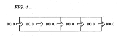
- Expression (3-30') that is, a case where a calculation result example of the present invention is illustrated in Fig. 4 .
- the temperatures are uniformly 100°C, and thus calculation results are supposed to be uniformly 100°C, but in the related art, the temperatures are not in an uniform distribution, and in the calculation result example of the present invention, the temperatures are uniformly 100°C.
- a secondary upwind scheme and a tertiary upwind scheme are schemes which are also usually used in fluid calculation.
- the detail description of these schemes is omitted herein, and ⁇ ab becomes Expression (3-32). That is, an interpolation function using grad (a gradient vector) of ⁇ a and ⁇ b is used.
- ⁇ ab ⁇ ab ⁇ a , ⁇ b , grad ⁇ ⁇ a , grad ⁇ ⁇ b , x a , x b , V a , V b , S ab , n ab , ⁇
- Fig. 5 is a schematic block diagram illustrating a configuration of a fluid simulation device 10 according to the first embodiment of the invention.
- the fluid simulation device 10 of this embodiment is a simulation device which simulates incompressible fluid by a finite volume method, and calculates a velocity and a pressure in a simulation region. That is, in this embodiment, a simulation device calculating a solution of a Navier-Stokes equation which is a transport equation relevant to a momentum will be described.
- the fluid simulation device 10 includes a cell configuration setting unit 101, a cell configuration memory unit 102, an initial condition setting unit 103, a velocity field memory unit 104, a velocity field acquisition unit 105, a velocity and pressure calculation unit 106, and a pressure field memory unit 107.
- the cell configuration setting unit 101 sets information relevant to cells into which the simulation region (a space) is divided, and stores the information in the cell configuration memory unit 102.
- the cell configuration memory unit 102 stores the information relevant to the cell which is set by the cell configuration setting unit 101.
- the information relevant to the cell includes cell information which is information of each cell, and intercell information which is information between adjacent cells.
- the initial condition setting unit 103 sets a velocity vector of each of the cells as initial conditions, and stores the velocity vector in the velocity field memory unit 104.
- the velocity field memory unit 104 stores the velocity vector of each of the cells which is set by the initial condition setting unit 103.
- the velocity field memory unit 104 also stores a velocity vector of each of the cells which is calculated by the velocity and pressure calculation unit 106 in each time step.
- the velocity field acquisition unit 105 reads out a velocity vector of each of the cells in a time step n-1 from the velocity field memory unit 104.
- the velocity and pressure calculation unit 106 calculates the velocity vector of each of the cells in the time step n-1 which is read from the velocity field memory unit 104 by the velocity field acquisition unit 105, and a velocity vector and a pressure of each of the cell in a target time step n by using the cell information stored in the cell configuration memory unit 102.
- the velocity and pressure calculation unit 106 stores the calculated velocity vector of each of the cells in the velocity field memory unit 104, and stores the calculated pressure in the pressure field memory unit 107. Furthermore, when the velocity vector and the pressure are calculated, the velocity and pressure calculation unit 106 uses a discretization equation in which the Navier-Stokes equation of the incompressible fluid and a continuity equation (referred to as an equation for mass conservation) of the incompressible fluid are discretized.
- the discretization equation of the Navier-Stokes equation of the incompressible fluid in this embodiment performs an operation including deformation of the advective term into a conservation form described later, and a term of correcting an error in the conservation form of the advective term with respect to the Navier-Stokes equation of the incompressible fluid. The detailed description thereof will be described later.
- the pressure field memory unit 107 stores the pressure of each of the cells which is calculated by the velocity and pressure calculation unit 106 in each time step.
- Fig. 6 is a conceptual diagram illustrating the cell of this embodiment.
- regions indicated by symbols R 1 to R 15 are 1st to 15th cells, respectively.
- each of the cells is in the shape of a polyhedron.
- the cells are arranged to fill the simulation regions without a gap.
- a boundary surface E 12 is a boundary surface between the cells R 1 and R 2 .
- a unit normal vector n 12 is a unit normal vector of the boundary surface E 12 .
- a distance ⁇ 12 is a distance from an intersection between a line connecting points C 1 and C 2 and the boundary surface E 12 to the representative point C 1 when a distance from the representative point C 1 to the representative point C 2 is 1.
- Fig. 7 is a diagram illustrating an example of the cell information stored in the cell configuration memory unit 102.
- the cell information includes cell IDs of all of the cells, representative point coordinates, and the volume.
- the cell information of the cell of which the cell ID is "0001" is the cell ID of "0001”
- the representative point coordinates of "15, 225, 214” and the volume of "24.3".
- the cell information of the cell of which the cell ID is "0002” is the cell ID of "0002”
- the cell information of the cell of which the cell ID is "2453” is the cell ID of "2453”
- three numerical values of the representative point coordinates are an x coordinate, a y coordinate, and a z coordinate.
- X n indicates the representative point coordinates of the cell of which the cell ID is n
- V n indicates the volume of the cell of which the cell ID is n.
- Fig. 8 is a diagram illustrating an example of the intercell information stored in the cell configuration memory unit 102.
- the intercell information includes a cell ID of a reference cell, a cell ID of a cell which is adjacent to the cell, an area of a boundary surface between these two cells, a unit normal vector of the boundary surface, and a distance ⁇ from an intersection between a straight line through representative points of these two cells and the boundary surface to a representative point of the reference cell.
- the unit normal vector is a unit vector having a length of "1".
- the distance is a distance when a distance between the representative points of the two cells is "1", and corresponds to ⁇ 12 of Fig. 6 .
- the intercell information relevant to the intercell between the cell of which the cell ID is "0001" and the cell of which the cell ID is "0005" is the cell ID of "0001", the cell ID of "0005", the area of "4.21458", the unit normal vector of "0.700243, 0.552466, 0.891941", and the distance of "0.422561".
- the intercell information relevant to the intercell between the cell of which the cell ID is "0001” and the cell of which the cell ID is “0102” is the cell ID of "0001", the cell ID of "0102", the area of "3.13352”, the unit normal vector of "0.584276, -0.617123, 0.527049", and the distance of "0.554878”, and the intercell information relevant to the intercell between the cell of which the cell ID is "2453” and the cell of which the cell ID is "2452” is the cell ID of "2453", the cell ID of "2452", the area of "3.31215", the unit normal vector of "0.335786, 0.814266, 0.473517", and the distance of "0.515486".
- Fig. 9 is a diagram illustrating an example of the velocity field information stored in the velocity field memory unit 104.
- the velocity field memory unit 104 stores velocity field information in an initial time step which is set as initial conditions, and velocity field information in each time step which is calculated by the velocity and pressure calculation unit 106.
- the example illustrated in Fig. 9 is the velocity field information in one time step.
- the velocity field information in one time step includes the cell ID of each cell and the velocity vector of each cell.
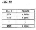
- Fig. 10 is a diagram illustrating an example of the pressure field information stored in the pressure field memory unit 107.
- the pressure field memory unit 107 stores pressure field information in each time step which is calculated by the velocity and pressure calculation unit 106.
- the example illustrated in Fig. 10 is the pressure field information in one time step.
- the pressure field information in one time step includes the cell ID of each cell and the pressure of each cell.
- the example of the pressure field information illustrated in Fig. 10 includes the cell ID of "0001" and the pressure of the cell of "1.28568", the cell ID of "0002" and the pressure of the cell of "1.22325", and the cell ID of "2453" and the pressure of the cell of "1.56846".
- Fig. 11 is a flowchart illustrating an operation of the fluid simulation device 10 of this embodiment.
- the cell configuration setting unit 101 stores the information (the cell information and the intercell information) relevant to the cell which is acquired from the outside in the cell configuration memory unit 102.
- the initial condition setting unit 103 stores the velocity field information of the initial time step set as the initial conditions which is acquired from the outside in the velocity field memory unit 104 (S1).
- the velocity field acquisition unit 105 sets the target time step to an initial value of "1" (S2).
- the velocity field acquisition unit 105 acquires the velocity field information of a step which is one step before the target time step from the velocity field memory unit 104 (S3).
- the velocity field acquisition unit 105 sets the initial time step to be the step which is one step before the target time step when the target time step is "1", and acquires the velocity field information of the initial time step from the velocity field memory unit 104.
- the velocity and pressure calculation unit 106 calculates each element of the matrix A and the vector b by using the velocity field information which is acquired by the velocity field acquisition unit 105 in Step S3.
- the vector ⁇ is a vector having each element of the velocity vector and the pressure of all of the cells in the target time step as an element. That is, the vector ⁇ has the number of cells x 4 elements.
- the linear simultaneous equation includes an equation in which a Navier-Stokes equation in each axis direction which is relevant to each of the cells is discretized, and an equation in which the continuity equation of the incompressible fluid which is relevant to each of the cells is discretized. That is, the linear simultaneous equation includes the same number of equations as the number of elements of the vector ⁇ , and thus the solution is able to be calculated. Furthermore, a method of calculating the matrix A and the vector b in Step S4 will be described later in detail.
- the velocity and pressure calculation unit 106 stores the velocity vector among the calculated elements of the vector ⁇ in the velocity field memory unit 104 as the velocity vector of the target time step.
- the velocity and pressure calculation unit 106 stores the pressure among the calculated elements of the vector ⁇ in the pressure field memory unit 107 as the pressure of the target time step (S5).
- the velocity and pressure calculation unit 106 determines whether or not termination conditions are satisfied (S6).
- the termination conditions for example, a condition in which the target time step is identical to a value which is set in advance, and the like are included.
- the velocity and pressure calculation unit 106 proceeds to Step S7 and increases the target time step by "1" (S7), and returns to Step S3. Accordingly, the processing is performed with respect to the next time step.
- Step S6 when it is determined that the termination conditions are satisfied (S6-Yes), the processing is terminated.
- the Navier-Stokes equation of the incompressible fluid in an i-th axis direction is denoted as Expression (4-1).
- the continuity equation of the incompressible fluid is denoted as Expression (4-2).
- an orthogonal coordinate system (a Cartesian coordinate system) is used as a coordinate system.
- t is a time.
- p is the pressure.
- p is the density.
- v is a dynamic coefficient of viscosity.
- a second term of a left member is an advective term.
- Expression (4-1) is an equation of momentum conservation in the i-th axis direction, and the density ⁇ of the fluid is constant due to the incompressible fluid, and thus in the advective term of Expression (4-1), a velocity u i in the i-th axis direction is advected.
- a sum of a second term (a viscosity term) and a third term (the external force) of a right member in Expression (4-1) is marked by -F (u), and the entire term of the right member will be described by using Expression (4-3) which is moved to a left member.
- the Navier-Stokes equation is volume integrated by the control volume, and the discretized equation is solved.
- an equation which is obtained by adding Expression (4-4) in which both members of Expression (4-2) which is the continuity equation are multiplied by the velocity u i to the Navier-Stokes equation, and by deforming the advective term into a form referred to as the conservation form is used.
- the deformation of the advective term into the conservation form is a deformation premised on a fact that the velocity vector satisfies Continuity Equation (4-2).
- Expression (4-8) is obtained.
- Expression (4-9) is identical to Expression (4-5) using the finite volume method of the related art except for including a third term of a left member, and the third term includes a term of correcting an error in the advective term of the conservation form (that is, -u i D).
- Expression (4-9) is volume integrated by the control volume
- Expression (4-10) is obtained.
- Expression (4-6) is volume integrated by the control volume
- Expression (4-11) is obtained.
- V is the volume of the control volume
- S is a surface of the control volume.
- n and u in a bold typeface in a second term of a left member of Expression (4-10) and in a first term of a left member of Expression (4-11) are a unit normal vector of the surface S of the control volume and the velocity vector, respectively.
- the unit normal vector n is a vector which is perpendicular to the surface S of the control volume, is outward, and has a length of "1".
- the boundary surface E 1k is a boundary surface between the cell R 1 and the cell R k .
- the class N 1 is a class of a cell ID of a cell which is adjacent to the cell R 1 .
- ⁇ t is a width of the time step.
- the area S 1k is an area of the boundary surface between the cell R 1 and the cell Rk.
- D 1 is an error in the continuity equation of the cell R 1 .
- u 1i is a component of the velocity in the i-th axis direction of the cell R 1 .
- u 1i (t - ⁇ t) is a component of the velocity in the i-th axis direction of the cell R 1 in the previous time step of the target time step.
- u 1ki is a component of the velocity in the i-th axis direction of the boundary surface E 1k .
- n 1k is a unit normal vector toward the cell R k of the boundary surface E 1k .
- u 1k is a velocity vector of the boundary surface E 1k .
- ⁇ k is a pressure of the cell R k .
- Expression (4-14) is one of first order equations configuring the linear simultaneous equation.
- Expression (4-14) includes multiplication between the velocities which are unknowns in a second term, and thus is not a first order equation. Therefore, approximation is performed in which the velocity vector of the previous time step is used as the velocity vector u 1k in the second term. In addition, for the sake of simple description, approximation in which the velocity vector of the previous time step is used is performed with respect to a discretization term of F (u).
- the velocity u 1ki of the boundary surface E 1k is interpolated from the velocity u 1i of the cell R 1 and the velocity u ki of the cell R k .
- a primary upwind scheme is used.
- n 1k is an outward vector which is seen from the cell R1.
- the velocity vector u 1k of the boundary surface E 1k is a velocity vector u 1k ' which is obtained by being interpolated from the velocity vector of each cell in the previous time step.
- a method is used in which a proportional distribution is performed with respect to velocity vectors u 1 ' and u 1 ' of the previous time step by using a distance ⁇ 1k stored in the cell configuration memory unit 102, as shown in Expression (4-16).
- u 1 ⁇ k ⁇ ⁇ ⁇ 1 ⁇ k ⁇ u 1 ⁇ ⁇ + 1 - ⁇ 1 ⁇ k ⁇ u k ⁇ ⁇
- Expression (4-14) becomes Expression (4-17).
- a class N 1 ' is a class having a cell number of a cell inflowing to the cell R 1 among cells adjacent to the cell R 1 as an element.
- Expression (4-17) becomes Expression (4-18), and thus becomes the first order equation in which an i axis component u 1i of the velocity of the cell R 1 and an i axis component u ki of the velocity of the adjacent cells R k , the pressure p of the cell R 1 are unknowns.
- Expression (4-2) which is the continuity equation is discretized with respect to the control volume V 1 of the cell R 1 , and the area S lk of the boundary surface E 1k (k ⁇ N 1 , the class N 1 is ⁇ 2, 3, 4, 11, 12, 13, and 14 ⁇ ), and is converted into the approximate equation by using the algebraic equation
- Expression (4-19) is obtained.
- Expression (4-19) becomes Expression (4-20), and thus becomes the first order equation in which each component of the velocity of the cell R 1 , and each component of the velocity of the adjacent cells R k are unknowns.
- Expressions (4-18) and (4-20) are equations relevant to the cell R 1 , and the same equation is able to be established with respect to each of other cells.
- the velocity and pressure calculation unit 106 sets each unknown coefficient of Expressions (4-18) and (4-20) with respect to all of the cells as an element of the matrix A, and sets a right member as an element of the vector b.
- the advective term is deformed into the conservation form by adding the continuity equation.
- the continuity equation includes the error D, and the discretization is performed by including the term of correcting the error D. Accordingly, even when the velocity of each time step does not completely satisfy the continuity equation, it is possible to suppress an influence due to the error, and thus an excellent simulation result is able to be obtained.
- the Navier-Stokes equation and the continuity equation are solved with coalition
- other equations may be solved with coalition.
- the discretization may be performed by including the term of correcting the error D of the advective term. Accordingly, it is possible to suppress an influence due to the error with respect to the equation, and thus an excellent simulation result is able to be obtained.
- the velocity and pressure calculation unit 106 calculates a solution of each time step
- an initial value of the solution is necessary at the time of using an iteration method such as a conjugate gradient method, and as the initial value, the solution of the previous time step may be used.
- the velocity field acquisition unit 105 acquires the pressure of the previous time step from the pressure field memory unit 107, and inputs the pressure to the velocity and pressure calculation unit 106.
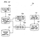
- FIG. 12 is a schematic block diagram illustrating a configuration of a fluid simulation device 10a according to the second embodiment of the invention.
- the fluid simulation device 10a of this embodiment is a simulation device which simulates the compressible fluid by a finite volume method, and calculates a velocity, a pressure, and a density in a simulation region.
- the fluid simulation device 10a includes the cell configuration setting unit 101, the cell configuration memory unit 102, an initial condition setting unit 103a, a density and velocity field memory unit 104a, a density-and velocity field acquisition unit 105a, a solution calculation unit 106a, and the pressure field memory unit 107.
- the same symbols 101, 102, and 107) are applied to parts corresponding to the respective parts of Fig. 5 , and thus the description thereof will be omitted.
- the initial condition setting unit 103a sets a velocity vector and a density of each cell as initial conditions, and stores the velocity vector and the density in the density and velocity field memory unit 104a.
- the density and velocity field memory unit 104a stores the velocity vector and the density of each of the cells which are set by the initial condition setting unit 103a.
- the density and velocity field memory unit 104a also stores a velocity vector and a density of each of the cells which are calculated by the solution calculation unit 106a in each time step.
- the solution calculation unit 106a calculates a solution relevant to the time step n
- the density and velocity field acquisition unit 105a reads out a velocity vector and a density of each of the cells in the time step n-1 from the density and velocity field memory unit 104a.
- the solution calculation unit 106a calculates the velocity vector and the density of each of the cells in the time step n-1 which are read from the density and velocity field memory unit 104a by the density and velocity field acquisition unit 105a, and a velocity vector, a pressure, and a density of each of the cells in the target time step n by using the cell information stored in the cell configuration memory unit 102.
- the solution calculation unit 106a stores the calculated velocity vector and density of each of the cells in the density and velocity field memory unit 104, and stores the calculated pressure in the pressure field memory unit 107.
- the solution calculation unit 106a solves a linear simultaneous equation including a discretization equation in which a Navier-Stokes equation of the compressible fluid is discretized, a discretization equation in which a continuity equation of the compressible fluid is discretized, and a discretization equation in which a state equation indicating a relationship between the density and the pressure is discretized calculates the velocity vector, the pressure, and the density of each of the cells.
- a solution method of a known linear simultaneous equation such as a conjugate gradient method is used.
- R is a gas constant
- T is a temperature (a thermal dynamics temperature).
- the temperature T is constant. Furthermore, the temperature T may not be constant, but may be known in advance. In addition, when the temperature T is not known in advance, a discretization equation in which the temperature T is a variable may be included in the linear simultaneous equation described above.
- Expression (4-24) becomes Expression (4-25) which is a conservation form.
- Expression (4-25) is identical to an equation used in the finite volume method of the related art except for including a third term of a left member, and the third term includes a term of correcting an error in the advective term of the conservation form (that is, -u i D).
- ⁇ ⁇ ⁇ u i ⁇ t + ⁇ u j ⁇ ⁇ ⁇ u i ⁇ x j - u i ⁇ D + ⁇ p ⁇ x i + ⁇ F u 0
- Expression (4-25) is volume integrated by the control volume
- Expression (4-26) is obtained.
- an equation in which a right member of Expression (4-22) is set to the error D is also volume integrated by the control volume
- Expression (4-27) is obtained.
- V is the volume of the control volume
- S is the surface of the control volume.
- n and u in a bold typeface in a second term of a left member of Expression (4-26) are a unit normal vector of the surface S of the control volume and a velocity vector, respectively.
- the unit normal vector n is a vector which is perpendicular to the surface S of the control volume, is outward, and has a length of "1".
- Expression (4-29) is assigned to a third term of Expression (4-28), Expression (4-30) is obtained. Similar to the first embodiment, a primary upwind scheme or the like is applied to Expression (4-30), and thus Expression (4-30) becomes a first order equation in which the velocity vector and the pressure are unknowns.
- Expression (4-30) is an equation relevant to the cell R1, and the same equation is able to be established with respect to each of other cells.
- the solution calculation unit 106a sets each unknown coefficient of Expression (4-30) with respect to all of the cells as the element of the matrix A, and sets a right member as the element of the vector b.
- the advective term is deformed into the conservation form by adding the continuity equation.
- the continuity equation includes the error D, and the discretization is performed by including the term of correcting the error D. Accordingly, even when the velocity of each time step does not completely satisfy the continuity equation, it is possible to suppress an influence due to the error, and thus an excellent simulation result is able to be obtained.
- the Navier-Stokes equation, the continuity equation, and the state equation are solved with coalition
- other equations may be solved with coalition.
- the discretization may be performed by including the term of correcting the error D of the advective term. Accordingly, it is possible to suppress an influence due to the error with respect to the equation, and thus an excellent simulation result is able to be obtained.
- the equation including the advective term the Navier-Stokes equation is included, and the fluid simulation devices 10 and 10a solving the equation are described.
- the equation including the advective term an equation for conservation of thermal energy of the continuum is included, and a continuum simulation device 10b solving the equation by a finite volume method will be described.
- a value input from the outside is used as a velocity vector of each time step in a simulation region. The velocity vector input from the outside may be calculated in advance by a simulation, or may be observation data or experiment data.
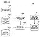
- Fig. 13 is a schematic block diagram illustrating a configuration of a continuum simulation device 1 according to the third embodiment of the invention.
- the continuum simulation device 10b of this embodiment includes the cell configuration setting unit 101, the cell confguration memory unit 102, a velocity field setting unit 103b, a velocity field memory unit 104b, a velocity field acquisition unit 105b, a solution calculation unit 106b, and a solution memory unit 107b.
- the same symbols (101 and 102) are applied to parts corresponding to the respective parts of Fig. 5 , and thus the description thereof will be omitted.
- the velocity field setting unit 103b stores a velocity vector of each of the cells which is input from the outside in the velocity field memory unit 104b. Furthermore, in this embodiment, as the velocity vector, a velocity vector of all time steps which become a simulation target is input.
- the velocity field memory unit 104b stores the velocity vector of each of the cells.
- the solution calculation unit 106b calculates a solution relevant to the time step n
- the velocity field acquisition unit 105b reads out the velocity vector of each of the cells in the time step n-1 from the velocity field memory unit 104b.
- the solution calculation unit 106b calculates a solution of an equation for conservation of thermal energy in the target time step n by using the velocity vector of each of the cells in the time step n-1 which is read from the velocity field memory unit 104b by the velocity field acquisition unit 105b, the cell information stored in the cell configuration memory unit 102, and a solution of the time step n-1 stored in the solution memory unit 107b.
- the solution calculation unit 106b stores the calculated solution in, the solution memory unit 107b as a solution of the target time step n.
- the solution calculation unit 106b uses a discretization equation in which an equation for energy conservation denoted by Expression (4-31) is discretized.
- the equation for energy conservation includes an advective term of a second term of a left member.
- the density ⁇ is not constant, and thus the solution calculation unit 106b uses a discretization equation in which Expression (4-31) is discretized, similar to the discretization of the Navier-Stokes equation in the second embodiment.
- the advective term is deformed into the conservation form by adding the continuity equation.
- the continuity equation includes the error D, and the discretization is performed by including the term of correcting the error D. Accordingly, even when the velocity of each time step which is input from the outside does not completely satisfy the discretized continuity equation, it is possible to suppress an influence due to the error, and thus an excellent simulation result is able to be obtained.
- an advection diffusion equation describing an advection diffusion phenomenon of a substance in the continuum also includes an advective term in which a concentration of the substance is advected as shown in Expression (4-32).
- a discretization equation may be solved in which the advection diffusion equation is discretized similarly to the equation for energy conservation.
- an equation for a stress field describing a stress field in the continuum also includes an advective term in which a deformation velocity of the continuum is advected as shown in Expression (4-33).
- a discretization equation may be solved in which the equation for a stress field is discretized similarly to the Navier-Stokes equation.
- a fourth embodiment of the present invention will be described with reference to the drawings.
- a fluid simulation device 10c which solves an equation including a plurality of advective terms by a finite volume method will be described.
- the fluid simulation device 10c which concurrently solves a Navier-Stokes equation and an equation for conservation of thermal energy is described.
- Fig. 14 is a schematic block diagram illustrating a configuration of the fluid simulation device 10c according to the fourth embodiment of the invention.
- the fluid simulation device 10c of this embodiment includes the cell configuration setting unit 101, the cell configuration memory unit 102, the initial condition setting unit 103, the velocity field memory unit 104, the velocity field acquisition unit 105, a solution calculation unit 106c, and a solution memory unit 107c.
- the same symbols 101 to 105 are applied to parts corresponding to the respective parts of Fig. 5 , and thus the description thereof will be omitted.
- the solution calculation unit 106c calculates a solution of a Navier-Stokes equation, a continuity equation, and an equation for conservation of thermal energy in the target time step n by using the velocity vector of each of the cells in the time step n-1 which is read from the velocity field memory unit 104 by the velocity field acquisition unit 105, the cell information stored in the cell configuration memory unit 102, and a solution of the time step n-1 stored in the solution memory unit 107c.
- the solution calculation unit 106c stores the calculated solution in the solution memory unit 107c as the solution of the target time step n. Furthermore, the solution calculation unit 106c stores the velocity among the calculated solutions in the velocity field memory unit 104.
- the solution calculation unit 106c uses the discretization equation of the first embodiment in which the Navier-Stokes equation and the continuity equation are discretized, and the discretization equation of the third embodiment in which the equation for conservation of thermal energy is discretized.
- the advective term when each of the equations including the advective term is discretized, the advective term is deformed into the conservation form by adding the continuity equation.
- the continuity equation includes the error D, and the discretization is performed by including the term of correcting the error D. Accordingly, even when the calculated velocity of time step does not completely satisfy the discretized continuity equation, it is possible to suppress an influence due to the error, and thus an excellent simulation result is able to be obtained.
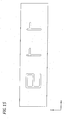
- Fig. 15 is a contour diagram illustrating a velocity field of a simulation target. That is, Fig. 15 is a contour diagram of the size of the velocity vector of each of the cells stored in the velocity field memory unit 104b by the velocity field setting unit 103b. Furthermore, the velocity field is calculated as a velocity field having no time change.
- a horizontal axis is an x axis
- a vertical axis is a y axis
- the size of the velocity field is 4 m in an x axis direction and 1 m in a y axis direction.
- the fluid uniformly flows from left to right at 1 m/s (a positive direction of the x axis), and there is a region in the shape of "err" in the velocity field in which the fluid flows from left to right at 1.2 m/s. Furthermore, the velocity in the y axis direction is 0.
- Fig. 16 is a contour diagram illustrating the size of a divergence of the velocity in the velocity field illustrated in Fig. 15 .
- a horizontal axis is an x axis
- a vertical axis is a y axis.
- the divergence of the velocity is identical to the left member of the continuity equation shown in Expression (2-3). That is, when the velocity field of Fig. 15 completely satisfies the continuity equation, the contour diagram of Fig. 16 will be uniformly "0". However, in the velocity field illustrated in Fig. 15 , there is the region in the shape of "err" in which the velocity is 1.2 m/s, and thus the velocity does not become "0" at right and left ends of the region.
- Fig. 17 is a contour diagram illustrating an example in which the temperature distribution of the velocity field illustrated in Fig. 15 is calculated by using the method of the related art. Furthermore, an initial value of the temperature distribution is uniformly 100°C, and the temperature distribution illustrated in Fig. 17 is a temperature distribution in a normal state.
- a horizontal axis is an x axis
- a vertical axis is a y axis
- a contour is a line in which a temperature of 83°C to 107°C is divided into 13 steps. As illustrated in Fig.
- Fig. 18 is a contour diagram illustrating an example in which the temperature distribution of the velocity field illustrated in Fig. 15 is calculated by the continuum simulation device 10b of the third embodiment.
- the initial value of the temperature distribution is uniformly 100°C
- the temperature distribution is a temperature distribution in a normal state.
- a horizontal axis is an x axis
- a vertical axis is a y axis
- a contour is a line in which a temperature of 83°C to 107°C is divided into 13 steps.
- a pseudo thermal sink/source does not occur, and thus the temperature is uniformly 100°C.
- the fluid of which the temperature is uniformly 100°C flows the temperature is uniformly 100°C even when time progresses, and thus it is understood that a preferred simulation result is able to be obtained by the continuum simulation device 10b.
- the fluid simulation devices 10 and 10a, and the continuum simulation device 10b may be realized by recording a program for realizing a function of each part or a function of a part thereof in Fig. 5 , Fig. 12 , Fig. 13 , and Fig. 14 in a computer readable recording medium, by reading the program recorded in the recording medium into a computer system, and by executing the program.
- the "computer system” herein includes hardware such as OS or peripheral equipment.
- the "computer readable recording medium” is a memory device such as flexible disk, magnetooptic disk, a portable medium such as ROM, and CD-ROM, and hard disk embedded in the computer system.
- the "computer readable recording medium” includes a medium dynamically storing the program for a short period of time such as a communication wire at the time of transmitting the program through a network such as Internet or a communication line such as a telephone circuit, and a medium storing the program for a constant period of time such as a volatile memory inside the computer system which is a server or a client at this time.
- the program described above may be a program for realizing a part of the function described above, or may be a program for realizing the function described above by being combined with the program which is recorded in the computer system in advance.
- the simulation device of the present invention is able to be used in a generation source estimation device disclosed in JP-A-2012-132824 .
- the generation source estimation device position information of observers disposed in a plurality of portions and measured concentration information are obtained, and on the basis of the information, an ejection spot is estimated from plurality of virtual ejection spots which is set in advance.
- the virtual ejection spot is a generation source, and a unit amount is ejected, what extent of concentration is measured by the observer (an influence function in the literature described above) is estimated with respect to each one of the virtual ejection spots, and the estimation result is used.
- the continuum simulation device described in the third embodiment described above which solves the advection diffusion equation is able to be used without using a setting method of the virtual ejection spot.
- the fluid simulation device which concurrently solves the Navier-Stokes equation and the advection diffusion equation is able to be used. Accordingly, it is possible to estimate the concentration measured by each observer with excellent accuracy, and thus it is also possible to estimate the generation source with excellent accuracy.
- the generation source may be gas or liquid.
Landscapes
- Engineering & Computer Science (AREA)
- Physics & Mathematics (AREA)
- Theoretical Computer Science (AREA)
- General Physics & Mathematics (AREA)
- General Engineering & Computer Science (AREA)
- Mathematical Physics (AREA)
- Geometry (AREA)
- Evolutionary Computation (AREA)
- Computer Hardware Design (AREA)
- Mathematical Analysis (AREA)
- Pure & Applied Mathematics (AREA)
- Mathematical Optimization (AREA)
- Data Mining & Analysis (AREA)
- Computational Mathematics (AREA)
- Algebra (AREA)
- Computing Systems (AREA)
- Databases & Information Systems (AREA)
- Software Systems (AREA)
- Fluid Mechanics (AREA)
- Management, Administration, Business Operations System, And Electronic Commerce (AREA)
Applications Claiming Priority (2)
| Application Number | Priority Date | Filing Date | Title |
|---|---|---|---|
| JP2012241260 | 2012-10-31 | ||
| PCT/JP2013/079175 WO2014069421A1 (fr) | 2012-10-31 | 2013-10-28 | Dispositif de simulation, procédé de simulation et programme |
Publications (2)
| Publication Number | Publication Date |
|---|---|
| EP2916247A1 true EP2916247A1 (fr) | 2015-09-09 |
| EP2916247A4 EP2916247A4 (fr) | 2016-04-20 |
Family
ID=50627326
Family Applications (1)
| Application Number | Title | Priority Date | Filing Date |
|---|---|---|---|
| EP13852061.4A Ceased EP2916247A4 (fr) | 2012-10-31 | 2013-10-28 | Dispositif de simulation, procédé de simulation et programme |
Country Status (5)
| Country | Link |
|---|---|
| US (1) | US20150234784A1 (fr) |
| EP (1) | EP2916247A4 (fr) |
| JP (1) | JP6164222B2 (fr) |
| CN (1) | CN104769593B (fr) |
| WO (1) | WO2014069421A1 (fr) |
Families Citing this family (6)
| Publication number | Priority date | Publication date | Assignee | Title |
|---|---|---|---|---|
| JP2017162269A (ja) * | 2016-03-10 | 2017-09-14 | ソニー株式会社 | 情報処理装置、電子機器、情報処理方法、及びプログラム |
| CN108805949B (zh) * | 2018-05-25 | 2022-04-12 | 杭州晟视科技有限公司 | 一种血流速度的修正方法、装置、终端和计算机存储介质 |
| CN112560326B (zh) * | 2019-09-26 | 2023-07-18 | 腾讯科技(深圳)有限公司 | 压力场的确定方法及装置 |
| CN111930491B (zh) * | 2020-09-29 | 2020-12-25 | 中国人民解放军国防科技大学 | 一种全局通信优化加速方法、装置和计算机设备 |
| CN113094878B (zh) * | 2021-03-23 | 2025-06-17 | 华中科技大学 | 一种用于铸造流动场数值模拟的并行计算方法及系统 |
| CN115169260B (zh) * | 2022-07-06 | 2025-10-10 | 中国南方电网有限责任公司超高压输电公司电力科研院 | 灭弧室直流燃弧耐受能力的判断方法、装置和计算机设备 |
Family Cites Families (10)
| Publication number | Priority date | Publication date | Assignee | Title |
|---|---|---|---|---|
| JP3721765B2 (ja) * | 1998-02-10 | 2005-11-30 | 三菱電機株式会社 | 3次元流れの有限要素解析法、解析装置、成形品を製造する製造方法および解析法のプログラムを記録した媒体 |
| JP2003255055A (ja) * | 2002-03-01 | 2003-09-10 | Hitachi Eng Co Ltd | 大気汚染発生源推定の環境シミュレーション方法およびシステム |
| US7117138B2 (en) * | 2003-03-14 | 2006-10-03 | Seiko Epson Corporation | Coupled quadrilateral grid level set scheme for piezoelectric ink-jet simulation |
| JP2006172136A (ja) * | 2004-12-15 | 2006-06-29 | Canon Inc | 情報処理装置、情報処理方法 |
| JP5132768B2 (ja) * | 2007-07-02 | 2013-01-30 | マグマ ギエッセレイテクノロジ ゲーエムベーハー | モールド充填プロセスのシミュレーションにおいて、粒子の統計的な配向分布を記述するための方法および装置。 |
| JP4875224B2 (ja) * | 2009-06-25 | 2012-02-15 | 旭硝子株式会社 | 物理量計算方法、数値解析方法、物理量計算プログラム、数値解析プログラム、物理量計算装置及び数値解析装置 |
| US8428922B2 (en) * | 2010-02-05 | 2013-04-23 | Seiko Epson Corporation | Finite difference level set projection method on multi-staged quadrilateral grids |
| KR101113301B1 (ko) * | 2010-03-23 | 2012-02-24 | 한국과학기술원 | 부피비를 이용한 다종 유체 해석 방법 및 기록 매체 |
| JP5433559B2 (ja) * | 2010-12-22 | 2014-03-05 | 三菱重工業株式会社 | 拡散物質の発生源推定装置および発生源推定方法 |
| US20130013277A1 (en) * | 2011-07-08 | 2013-01-10 | Jiun-Der Yu | Ghost Region Approaches for Solving Fluid Property Re-Distribution |
-
2013
- 2013-10-28 JP JP2014544502A patent/JP6164222B2/ja not_active Expired - Fee Related
- 2013-10-28 WO PCT/JP2013/079175 patent/WO2014069421A1/fr not_active Ceased
- 2013-10-28 EP EP13852061.4A patent/EP2916247A4/fr not_active Ceased
- 2013-10-28 CN CN201380056818.9A patent/CN104769593B/zh not_active Expired - Fee Related
-
2015
- 2015-04-29 US US14/699,858 patent/US20150234784A1/en not_active Abandoned
Also Published As
| Publication number | Publication date |
|---|---|
| JPWO2014069421A1 (ja) | 2016-09-08 |
| CN104769593B (zh) | 2018-09-21 |
| US20150234784A1 (en) | 2015-08-20 |
| JP6164222B2 (ja) | 2017-07-19 |
| EP2916247A4 (fr) | 2016-04-20 |
| WO2014069421A1 (fr) | 2014-05-08 |
| CN104769593A (zh) | 2015-07-08 |
Similar Documents
| Publication | Publication Date | Title |
|---|---|---|
| EP2916247A1 (fr) | Dispositif de simulation, procédé de simulation et programme | |
| Jofre et al. | Conservation properties of unstructured finite-volume mesh schemes for the Navier-Stokes equations | |
| Trias et al. | A self-adaptive strategy for the time integration of Navier-Stokes equations | |
| Ling et al. | Analysis of turbulent scalar flux models for a discrete hole film cooling flow | |
| Hefny et al. | CFD analysis of pollutant dispersion around buildings: Effect of cell geometry | |
| Darwish et al. | A fully coupled Navier-Stokes solver for fluid flow at all speeds | |
| Lee et al. | Film cooling performance of cylindrical holes embedded in a transverse trench | |
| Réthoré et al. | A discrete force allocation algorithm for modelling wind turbines in computational fluid dynamics | |
| Tafarojnoruz et al. | Large eddy simulation of the turbulent flow field around a submerged pile within a scour hole under current condition | |
| Antuono et al. | The damping of viscous gravity waves | |
| Ling et al. | Experimentally informed optimization of turbulent diffusivity for a discrete hole film cooling geometry | |
| Salehi et al. | Experimental determination and computational fluid dynamics predictions of pressure loss in close-coupled elbows (RP-1682) | |
| Mangani et al. | A fully coupled OpenFOAM® solver for transient incompressible turbulent flows in ALE formulation | |
| Alonso et al. | Robust reduced order modeling of heat transfer in a back step flow | |
| Barbosa-Saldaña et al. | Flow over a three-dimensional horizontal forward-facing step | |
| Paniagua et al. | Large eddy simulations (LES) on the flow and heat transfer in a wall-bounded pin matrix | |
| Wang et al. | Numerical simulation of one-dimensional two-phase flow using a pressure-based algorithm | |
| Albuquerque et al. | Residual least-squares error estimate for unstructured h-adaptive meshes | |
| Storti et al. | A FFT preconditioning technique for the solution of incompressible flow on GPUs | |
| Chatterjee et al. | Convective transport around rows of square cylinders arranged in a staggered fashion at moderate Reynolds number | |
| Wu et al. | A numerical scheme to reduce numerical diffusion for advection-dispersion modeling: validation and application | |
| Hsieh et al. | Flow characteristics of three-dimensional microscale backward-facing step flows | |
| Maruszewski et al. | Grid generation and its application to separated flows | |
| Karbon et al. | Large-eddy simulation of the flow in Z-Shape duct | |
| JP2006258391A (ja) | 浮力を伴う乱流の流体的及び熱的諸特性の推定方法及び推定プログラム |
Legal Events
| Date | Code | Title | Description |
|---|---|---|---|
| PUAI | Public reference made under article 153(3) epc to a published international application that has entered the european phase |
Free format text: ORIGINAL CODE: 0009012 |
|
| 17P | Request for examination filed |
Effective date: 20150430 |
|
| AK | Designated contracting states |
Kind code of ref document: A1 Designated state(s): AL AT BE BG CH CY CZ DE DK EE ES FI FR GB GR HR HU IE IS IT LI LT LU LV MC MK MT NL NO PL PT RO RS SE SI SK SM TR |
|
| AX | Request for extension of the european patent |
Extension state: BA ME |
|
| DAX | Request for extension of the european patent (deleted) | ||
| RA4 | Supplementary search report drawn up and despatched (corrected) |
Effective date: 20160323 |
|
| RIC1 | Information provided on ipc code assigned before grant |
Ipc: G06F 17/50 20060101ALI20160317BHEP Ipc: G06F 19/00 20110101AFI20160317BHEP |
|
| RAP1 | Party data changed (applicant data changed or rights of an application transferred) |
Owner name: AGC INC. |
|
| 17Q | First examination report despatched |
Effective date: 20181203 |
|
| REG | Reference to a national code |
Ref country code: DE Ref legal event code: R003 |
|
| STAA | Information on the status of an ep patent application or granted ep patent |
Free format text: STATUS: THE APPLICATION HAS BEEN REFUSED |
|
| 18R | Application refused |
Effective date: 20200530 |