EP2954308B1 - Verfahren zur messung der eigenschaften von mikroporösem material in mehreren massstäben - Google Patents
Verfahren zur messung der eigenschaften von mikroporösem material in mehreren massstäben Download PDFInfo
- Publication number
- EP2954308B1 EP2954308B1 EP14749191.4A EP14749191A EP2954308B1 EP 2954308 B1 EP2954308 B1 EP 2954308B1 EP 14749191 A EP14749191 A EP 14749191A EP 2954308 B1 EP2954308 B1 EP 2954308B1
- Authority
- EP
- European Patent Office
- Prior art keywords
- pressure
- sample
- permeability
- gas
- test
- Prior art date
- Legal status (The legal status is an assumption and is not a legal conclusion. Google has not performed a legal analysis and makes no representation as to the accuracy of the status listed.)
- Active
Links
Images









Classifications
-
- G—PHYSICS
- G01—MEASURING; TESTING
- G01N—INVESTIGATING OR ANALYSING MATERIALS BY DETERMINING THEIR CHEMICAL OR PHYSICAL PROPERTIES
- G01N15/00—Investigating characteristics of particles; Investigating permeability, pore-volume or surface-area of porous materials
- G01N15/08—Investigating permeability, pore-volume, or surface area of porous materials
- G01N15/082—Investigating permeability by forcing a fluid through a sample
-
- G—PHYSICS
- G01—MEASURING; TESTING
- G01N—INVESTIGATING OR ANALYSING MATERIALS BY DETERMINING THEIR CHEMICAL OR PHYSICAL PROPERTIES
- G01N15/00—Investigating characteristics of particles; Investigating permeability, pore-volume or surface-area of porous materials
- G01N15/08—Investigating permeability, pore-volume, or surface area of porous materials
-
- G—PHYSICS
- G01—MEASURING; TESTING
- G01N—INVESTIGATING OR ANALYSING MATERIALS BY DETERMINING THEIR CHEMICAL OR PHYSICAL PROPERTIES
- G01N15/00—Investigating characteristics of particles; Investigating permeability, pore-volume or surface-area of porous materials
- G01N15/08—Investigating permeability, pore-volume, or surface area of porous materials
- G01N15/0806—Details, e.g. sample holders, mounting samples for testing
-
- G—PHYSICS
- G01—MEASURING; TESTING
- G01N—INVESTIGATING OR ANALYSING MATERIALS BY DETERMINING THEIR CHEMICAL OR PHYSICAL PROPERTIES
- G01N15/00—Investigating characteristics of particles; Investigating permeability, pore-volume or surface-area of porous materials
- G01N15/08—Investigating permeability, pore-volume, or surface area of porous materials
- G01N15/082—Investigating permeability by forcing a fluid through a sample
- G01N15/0826—Investigating permeability by forcing a fluid through a sample and measuring fluid flow rate, i.e. permeation rate or pressure change
-
- G—PHYSICS
- G01—MEASURING; TESTING
- G01N—INVESTIGATING OR ANALYSING MATERIALS BY DETERMINING THEIR CHEMICAL OR PHYSICAL PROPERTIES
- G01N15/00—Investigating characteristics of particles; Investigating permeability, pore-volume or surface-area of porous materials
- G01N15/08—Investigating permeability, pore-volume, or surface area of porous materials
- G01N15/088—Investigating volume, surface area, size or distribution of pores; Porosimetry
-
- G—PHYSICS
- G01—MEASURING; TESTING
- G01N—INVESTIGATING OR ANALYSING MATERIALS BY DETERMINING THEIR CHEMICAL OR PHYSICAL PROPERTIES
- G01N33/00—Investigating or analysing materials by specific methods not covered by groups G01N1/00 - G01N31/00
- G01N33/24—Earth materials
-
- G—PHYSICS
- G01—MEASURING; TESTING
- G01N—INVESTIGATING OR ANALYSING MATERIALS BY DETERMINING THEIR CHEMICAL OR PHYSICAL PROPERTIES
- G01N7/00—Analysing materials by measuring the pressure or volume of a gas or vapour
Definitions
- the present application relates to methodology for measuring properties of microporous material such as reservoir rock and core samples extracted from geologic formations.
- Permeability of a material is a macroscopic property of the material which characterises the ease with which a fluid can be made to flow through the material by an applied pressure gradient.
- permeability is the fluid conductivity of the material.
- Porosity is the fraction of the bulk volume of the material that is occupied by voids.
- the total fractional volume of pores in the material can be referred to as total porosity; the fractional volume of only those pores in the material which, under given conditions, are interconnected is known as effective porosity. Only effective porosity contributes to the permeability of the material.
- the term "porosity" is used to describe the effective porosity of the material.
- the method is based on fitting of experimental curves to the square-root of time asymptote of the analytic solution at t ⁇ 0 and to the single-exponent asymptote of the analytic solution at t ⁇ . Based on the results of this comparison, performed using numerical modeling, the authors suggest that fitting of the late-time behavior results in better accuracy in the inferred permeability.
- the valve connecting the two volumes is opened and the transient process of pressure equilibration is recorded and interpreted to infer the new porosity and permeability of the sample under the newly applied stress.
- the paper compares the permeability values obtained by ISPP and the conventional pulse decay method on plugs. During pressure decay gas flows through the length of a plug sample, by controlling the pressure difference at both ends of the sample, under controlled conditions of confining stress. Cui et al. report the difference in the ISPP and pulse decay permeabilities to be up to two orders of magnitude, which is explained by the intrinsic heterogeneity of samples.
- the method relies on the assumption that after initial liquid saturation of rock fragments at atmospheric pressure the fragments still have some of their pore volume ( ⁇ 10%) uniformly filled by a trapped gas; which is trapped in the form of multiple pockets of gas isolated by liquid.
- the residual gas volume provides compressibility that enables the flow of liquid into the particles.
- Both cumulative injected volume and fluid pressure in the cell are recorded at about 500 Hz sampling rate, and the permeability is interpreted based on comparisons with numerical simulations.
- the authors report a wide range of measureable permeabilities from 0.1 to 2000 milli-Darcy. Unfortunately, due to the high viscosity of the liquids used, compared to gas, the measurable permeability range of this system is only suitable for conventional reservoir rocks and not suitable for sub-micro Darcy unconventional reservoir rocks.
- the first procedure is based on the estimation of the characteristic pore size h of the sample, using known porosimetry methods. With this input, the value of liquid permeability is determined from a look-up table, pre-calculated using Lattice Boltzmann Method (LBM) simulations, which provides a one-to-one relationship between h and permeability.
- LBM Lattice Boltzmann Method
- the second procedure is based on matching the experimental values of routine pressure decay permeability on rock fragments and measured at different pore pressures, with theoretical LBM curves defining variation of apparent permeability with pore pressure.
- the step-by-step procedures presented in his work have three critical drawbacks that make the method impractical for determining absolute permeability values: 1) the one-to-one relationship between the pore size and permeability is too strong an assumption for natural materials with heterogeneous fabric, which will not hold for combinations of pore sizes with different geometries; 2) the paper indicates that the estimation of permeability from pore size using the analytic formula and the look-up table is interchangeable in case of large channels and nearly Darcy flow; yet, the difference is several orders of magnitude; 3) the relationship between the sample's permeability and the characteristic pore size should include the porosity of the sample, otherwise the density of flow channels per unit area is not determined.
- Permeability measurements of ultra low permeability, microporous materials present challenges, particularly, in heterogeneous unconventional reservoir rocks.
- coring and core handling of heterogeneous rock samples can create extensive microcracking.
- the presence of these microcracks directly affects the permeability measured, and the lower the rock permeability, the larger the effect of the induced microcracks.
- This effect is most prevalent for laminated, low permeability, organic-rich, mudstones, where the organic to mineral contact and the interfaces associated with the laminated fabric are weak contacts that are prone to part during unloading. (This effect is less important for conventional, higher permeability rocks.)
- conventional permeability measurements developed for homogeneous media have focused on the evaluation of a single representative value of permeability, without accounting for the distribution of permeabilities. The resulting consequences are that the "single permeability" is ill-defined and not necessarily representative of the rock containing the distribution of permeabilities.
- a third challenge to measuring permeability if more conventional fluid flow through plug samples is used for permeability measurements, is the difficulty of flowing through the samples. It can take impractical times to detect measureable flow through samples of standard size (e.g., 1 to 1.5 inch (25.4 to 38.1 mm) in diameter and 1 to 2 inches (25.4 to 50.8 mm) in length). During these long periods of time, it may simply be impossible to not have small leaks that distort the flow measurements and thereby yield incorrect permeability inferences.
- the method using crushed fragments of sample tends to be the standard method most often used for measuring permeability in ultra-low permeability rocks.
- the crushed sample fragments' measured permeabilities do not represent the mean value of the whole permeability distribution of the rock before it was crushed, unless a further calibration or correction is made to these measurements.
- the invention relates to a method for characterizing properties of a manufactured rock sample according to claim 1.
- Illustrative embodiments of the present invention are directed to a method for characterising properties of a manufactured rock sample that employs first and preferably second test apparatus.
- the first test apparatus includes a sample holder and associated upstream and downstream reservoirs each associated with at least one pressure sensor, wherein the sample holder is configured to contain the manufactured rock sample under pressurized confinement and allows for a pulse of test fluid to flow through the manufactured rock sample contained within the sample holder, and the pressure sensor of the first test apparatus are configured to measure pressure of the upstream and downstream reservoirs as the pulse of test fluid flows through the manufactured rock sample contained within the sample holder.
- the second test apparatus preferably includes a sample cell and associated pressure sensor, wherein the sample cell has a configuration where the sample cell is filled with test fluid under pressure and isolated from other parts of the second test apparatus, and wherein the pressure sensor of the second test apparatus has a configuration that measures pressure of the sample cell when the sample cell is isolated from other parts of the second test apparatus.
- the first test apparatus is used with the manufactured rock sample loaded within the sample holder to characterise bulk properties of the manufactured rock sample.
- the second test apparatus is used with the manufactured rock sample loaded within the sample cell to characterise bulk properties of the manufactured rock sample.
- the manufactured rock sample is divided into a number of pieces of different sizes, and the pieces are partitioned into size-groups of different sizes. A sequence of operations is performed for each given size-group of pieces, wherein the sequence of operations includes:
- the bulk and size-group properties of the manufactured rock sample can be combined for user visualization of the combined properties of the manufactured rock sample.
- the bulk properties can be selected from the group consisting of bulk volume, bulk density, porosity, permeability, grain volume, grain density, and effective density-based porosity.
- the computational model is based on an analytical decay function that includes three parameters ⁇ , ⁇ and ⁇ , where the parameter ⁇ is a storage coefficient that defines the ratio of pore volume to dead volume in the sample under test, the parameter ⁇ relates to the final pressure in the sample cell when pressure inside and outside of the pore volume of the sample under test has stabilized, and parameter ⁇ is a relaxation time.
- the properties of the given size-group of pieces of the manufactured rock sample can be selected from the group consisting of bulk volume based on value of the parameter ⁇ for the matching pressure curve, porosity based on value of the parameter ⁇ for the matching pressure curve, permeability based on the parameter ⁇ for the matching pressure curve, grain volume based on the bulk volume and the porosity, bulk density based on bulk volume, grain density based on grain volume, and effective density-based porosity based on bulk and grain density.
- the processing the pressure data derives corrected pressure values that are matched to the set of pressure curves derived from the computational model in order to identify the matching pressure curve.
- the pieces of the manufactured rock sample can be fragments of uncontrolled shape with sizes corresponding to the radius of such fragments.
- the pieces of the manufactured rock sample can have a controlled shape (such as slices of a core sample with varying thickness) with sizes corresponding to thickness of the controlled shape.
- coring and core handling of heterogeneous rock samples can create extensive microcracking.
- the presence ofmicrocracking directly affects the real permeability of the rock, and the lower the rock permeability, the larger the effect of the induced microcracking.
- This effect is most important for laminated, low permeability, organic-rich, mudstones, where the organic to mineral contact and the interfaces associated with the laminated fabric are weak contacts that are prone to part during unloading. This effect is less important for conventional, higher permeability rocks.
- Crushing of the rock into fragments also has the advantage that tests can be conducted on a broader distribution of samples, including fragments from cores, parted sections of core sections, parted rotary sidewall plugs, and potentially drill cuttings, given that the measurements do not depend on the mechanical integrity and quality of cylindrical samples.
- the measurement of average permeability is considered to be a characteristic conductivity index of the rock to be used for direct comparison between different rocks.
- the permeability distribution characterisation is conducted on samples selected based on differences in their composition, texture, and average permeability which allows one to focus only on the rocks that are critical for the overall productivity of the reservoir.
- the first one (which is referred to herein as a "manufactured sample”) has a well-defined and controlled shape and requires material of sufficiently good quality to allow the manufacturing of samples with controlled shape (for example by drilling small cylindrical plugs or cutting small cubic samples with a diamond saw, out of a larger sample of whole core).
- the second one (which is referred to herein as a "fragmented sample”) is made up of a fragmented medium without a well-defined and controlled shape, and thus relaxes the condition of material competence. Protocols for testing permeability distribution in fragmented samples and manufactured samples are described separately herein.
- the permeability measurements described herein rely on pressure diffusion in porous samples and are limited by two clear experimental boundaries that define the permeability range that can be resolved by the measurements.
- the first experimental boundary is associated with the fastest pressure response related to diffusion of gas into fragments that can be measured, without being affected by initial gas flows at initiation of the test, gas expansion and compression, and related thermal effects.
- This high permeability limit defines the maximum measurable permeability and is difficult to extend because of the finite time of initial gas flow and because adiabatic heating and cooling of gas during the initial flow takes finite time to dissipate. Permeabilities higher than this limit cannot be detected by the equipment.
- the second experimental boundary is a low permeability limit defined by the maximum practical duration of the test and potential impact of unavoidable equipment leaks. Permeabilities equal to or lower than this limit cannot be detected by the equipment.
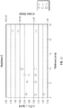
- Figure 1 shows the effect of particle size on the resolution of permeability by pressure decay systems. Specifically, Figure 1 shows a plot of measureable permeability versus particle radius, for narrow particle size distributions.
- the characteristic diffusion time which cannot be shorter or longer than certain limits, is controlled by the gas viscosity and compressibility, rock porosity, permeability, and the square of the rock fragment size. This means that the fragment size has the biggest impact on the measurable range of permeability.
- the upper and lower measurable permeability limits are shown in solid (upper limit) and dotted (lower limit) lines. The dependence of permeability resolution with particle size is given by the slopes of these lines.
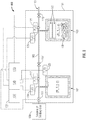
- FIG. 2 is a schematic diagram of an isolated cell pressure decay testing apparatus 100 in accordance with the present application.
- the apparatus 100 includes a housing 151 that houses a sealed cylindrical vessel referred to as the reference cell 101 and another sealed cylindrical vessel referred to as the sample cell 103.
- the volumes of both the reference cell 101 and the sample cell 103 are known.
- Tubing network 105 provides a closed fluid path between the internal volumes of the reference cell 101 and the sample cell 103.
- An electronically-controlled intermediate valve 107 is integral to the tubing network 105 and disposed between the reference cell 101 and the sample cell 103 as shown.
- the tubing network 105 also provides a closed fluid path between the reference cell 101 and a source of testing gas 109.
- An electronically-controlled intake valve 111 is integral to the tubing network 105 and disposed between the source of testing gas 109 and the reference cell 101 as shown.
- the source of testing gas 109 can employ a pressure regulator that releases the testing gas into the tubing network 105 at constant pressure.
- the tubing network 105 also provides a closed fluid path between the sample cell 103 and an exhaust port 113 that vents to atmosphere.
- An electronically-controlled exhaust valve 115 is integral to the tubing network 105 and disposed between the sample cell 103 and the exhaust port 113 as shown.
- the electronically-controlled valves 107, 111, 115 preferably have a fast response time that is on the order of tens of milliseconds (such as 10 milliseconds) or faster.
- the tubing network 105 can be implemented by solid piping made of low compressibility, non-corrosive, leak-proof material (such as stainless steel, various metal alloys, or any other existing or future materials satisfying the aforementioned requirements).
- the solid piping implementation can provide for flexibility in terms of replacing the components, such as switching the sizes and shapes of the reservoir and sample cells as necessary.
- the tubing network 105 can be implemented as a single piece manifold of low compressibility, non-corrosive, leak-proof material (such stainless steel, various metal alloys, or any other existing or future material satisfying the aforementioned requirements) which has output ports for all sensors, valves, and cells.
- the manifold implementation can provide a reduced risk of leaks.
- a pressure sensor 117 is fluidly coupled to the reference cell 101 and is configured to measure pressure of the reference cell 101 over time.
- a temperature sensor 119 (such as a thermocouple) is fluidly coupled to the reference cell 101 and is configured to measure temperature of the reference cell 101 over time.
- the pressure sensor 117 and the temperature sensor 119 preferably provide a fast response time on the order of tens of milliseconds (such as 10 milliseconds) or less.
- a pressure sensor 121 is fluidly coupled to the sample cell 103 and is configured to measure pressure of the sample cell 103 over time.
- a temperature sensor 123 (such as a thermocouple) is fluidly coupled to the sample cell 103 and is configured to measure temperature of the sample cell 103 overtime.
- the pressure sensor 121 and the temperature sensor 123 preferably provide a fast response time on the order of tens of milliseconds (such as 10 milliseconds) or less.
- An additional temperature sensor 125 (such as a thermocouple) is positioned at or near the center of the housing 151 and is configured to measure the average temperature of the system.
- the housing 151 encloses all the piping, valves, sensors, and the two cells, and can provide thermal insulation to the system and reduce temperature variations caused by external sources.
- the electronically-controlled valves 107, 111, 115, the pressure sensors 117, 121 and the temperature sensors 119, 123, 125 are electrically coupled to a data processing system 131.
- the data processing system 131 includes a valve control and interface module 133 that is configured to communicate electronic signals to the valves 107, 111, 115 for control over the operation of the valves 107, 111, 115 during operation of the system as described herein.
- the data processing system 131 also includes a data acquisition module 135 that samples the electrical signals output by the pressure sensors 117, 121 and the temperature sensors 119, 123, 125 overtime and stores electronic data that represents such output signals.
- the data acquisition module 135 can perform analog-to-digital conversion of the signals output by the pressure sensors 117, 121 and the temperature sensors 119, 123, 125 as needed. Alternatively, such analog-to-digital conversion can be performed by the pressure sensors 117, 121 and/or the temperature sensors 119, 123, 125 themselves.
- the data processing system 131 also includes a data analysis module 137 that processes data representing the output of the pressure sensors 117, 121 and the temperature sensors 119, 123, 125 to characterise certain properties of the porous material under test as described herein.
- the sample cell 103 can be loaded with a set of steel billets 127 of known volume along with a porous material under test (i.e., a porous sample) 129.
- the sample cell 103 can be equipped with a sliding lid, which can be moved by highpressure air or other suitable means under control of a manual switch in order to open or close the sliding lid to facilitate the loading and unloading of the billets 127 and the sample 129 into the interior space of the sample cell 103.
- the sample cell 103 can be put on a moving stand, which is moved up or down by a manual switch and pushed against a fixed lid or flat manifold surface at the top position to close the cell.
- the sealing mechanism between the sample cell and the sliding lid or between the sample cell and the manifold has to satisfy the following conditions: insignificant changes in the volume of the sample cell during multiple open/close cycles and due to pressure changes in the sample cell; sufficient flexibility to isolate the sample cell from the atmosphere; no leakage of the testing gas through the seal.
- Such seal can be implemented, for example, using commercially available O-rings with small cross-section diameter (3 mm or less cross-section diameter; ring diameter can be varied, typically in the order of 30 mm) made of non-porous leak-tight rubber or using a custom-designed polytetrafluoroethylene sealing post attached to the sample cell. Other existing or future materials satisfying the aforementioned requirement can be used in manufacturing of the sealing post.
- the design of the tubing network 105 and the cells 101, 103 incorporates optimization of their thermal properties, which satisfies the following requirements:
- the reference cell 101, the sample cell 103, and the tubing network 105 must be sufficiently rigid in order to ensure negligible variations of system volumes due to gas compression/expansion.
- the testing apparatus of Figure 2 can be configured to measure porosity and permeability of a sample at a predetermined elevated pressure as follows. Initially, the valve control and interface module 133 controls the intermediate valve 107 to assume a closed position in order to isolate the reference cell 101 from the sample cell 103, and the sample cell 103 is loaded with the rock sample and closed at atmospheric pressure. The intake valve 111 is controlled to assume an open position to fluidly couple the source of testing gas 109 to the reference cell 101 in order to fill the reference cell 101 with testing gas at the predetermined elevated pressure of the test. After filling the reference cell 101 with testing gas, the valve control and interface module 133 controls the intake valve 111 to assume a closed position to isolate the reference cell 101.
- the valve control and interface module 133 controls the intermediate valve 107 to assume an open position for a very short period of time (typically on the order of tens or hundreds of milliseconds), which is sufficient to flow substantial amounts of the testing gas from the reference cell 101 into the sample cell 103.
- a very short period of time typically on the order of tens or hundreds of milliseconds
- the pressure in the reference cell 101 falls rapidly, due to gas expansion from the reference cell 101 into the free volume of the sample cell 103.
- the time interval that the intermediate valve 107 remains open to allow flow of testing gas from the reference cell 101 into the sample cell 103 must satisfy several conditions. First, it has to be long enough to create a substantial pressure increase in the sample cell 103.
- valve control and interface module 133 controls the intermediate valve 107 to assume a closed position that isolates both the reference cell 101 and the sample cell 103.
- the gas pressure in the sample cell 103 begins to decrease at a slower rate due to diffusion of gas into the porous sample.
- the valve control and interface module 133 controls the exhaust valve 115 to assume an open position that fluidly couples the sample cell 103 to the exhaust port 113 for a short period of time in order to reduce the pressure in the sample cell 1 03 to atmospheric.
- the time interval that exhaust valve 115 remains open has to be sufficiently long to drop pressure completely and at the same time sufficiently short to prevent diffusion and mixing of air with the testing gas in the sample cell.
- the optimal duration of the exhaust cycle has to be determined for particular equipment design and testing gas.
- the exhaust cycle has to provide final pressure in the empty sample cell within 1 psi (0.07 kg/square cm) of atmospheric.
- the typical exhaust time can be around 1-4 seconds.
- valve control and interface module 133 controls the exhaust valve 115 to assume a closed position that isolates the sample cell 103. After the exhaust valve 115 is closed, the gas pressure in the sample cell 103 increases as gas diffuses out of the porous sample 129 into the interior space of sample cell 103. These operations are referred to as the degassing stage and continue for a time period T degas .
- the data acquisition module 135 cooperates with the pressure sensor 117 and the temperature sensor 119 to measure and record the temperature and pressure of the reference cell 101 over time.
- the data acquisition module 135 also cooperates with the pressure sensor 121 and the temperature sensor 123 to measure and record the temperature and pressure of the sample cell 103 over time.
- the data acquisition module 135 cooperates with the temperature sensor 125 to measure and record the average temperature of the system over time.
- the data analysis module 137 processes data representing the output of the pressure sensors 117, 121 and the temperature sensors 119, 123, 125 to characterise permeability and porosity of the porous material under test.
- Such analysis involves matching data that represents the transient pressure of the sample cell 103 over time (particularly during the time period T decay of the pressure decay stage and during the time period T degas of the degassing stage) to pressure curves (i.e., pressure data) generated by a computational model where the pressure curves are related to materials of known porosity and permeability characteristics.
- the permeability and porosity of the porous material under test can be derived from the porosity and permeability characteristics of the material related to the best-matching pressure curve.
- the isolated configuration of the sample cell 103 during both the pressure decay stage and the degassing stage has multiple advantages.
- the dead volume (cell volume minus volume of particles) is decreased by a factor of approximately three or more. This increases the observed pressure variation due to gas diffusion into the pore space, and also increases the accuracy and low limit of porosity and permeability measurements.
- the thermal mass of gas in the cell compared to the thermal mass of the cell, is reduced. As a consequence, the temperature variations in the cell are also reduced.
- the observed pressure variations due to thermal adiabatic effects in the gas are reduced compared to pressure variations due to gas diffusion. This is so because the reference cell, which has a larger relative thermal mass of gas than the sample cell and larger temperature fluctuations, is isolated from the sample cell.
- the single cell system is simple to model numerically and analytically.
- the operation of the valve control and interface module 133 is implemented by a testing script specified as an ASCII text file.
- the testing script is loaded and executed by the valve control and interface module 133 to perform automatic control operations as specified by the testing script.
- An exemplary testing script that measures porosity and permeability of a porous sample at a predetermined elevated pressure includes the following steps. It is assumed that the sample cell 103 is loaded with the rock sample.
- test script controls the intermediate valve 107 to assume a closed position in order to isolate the reference cell 101 from the sample cell 103, and the intake valve 111 is controlled to assume an open configuration to fluidly couple the source of testing gas 109 to the reference cell 101 in order to fill the reference cell 101 with testing gas at an initial elevated (for example, at approximately 2 atmospheres absolute pressure or higher).
- Each flushing cycle consists of flowing the testing gas from the reference cell 101 to the sample cell 103, by opening and then closing the intermediate valve 107, and releasing the gas mixture through the exhaust port 113 to atmosphere by opening and then closing the exhaust valve 115.
- the relative concentration of air and the testing gas in the dead volume becomes negligible (apart from the gas in the pore space with limited permeability), and the pressure in the isolated sample cell 103 is near atmospheric pressure.
- the test script controls the intermediate valve 107 to assume a closed position in order to isolate the reference cell 101 from the sample cell 103, and the intake valve 111 is controlled to assume an open position to fluidly couple the source of testing gas 109 to the reference cell 101 in order to fill the reference cell 101 with testing gas at the predetermined elevated pressure of the test.
- the intake valve 111 is controlled to assume a closed position to isolate the reference cell 101.
- test script performs a wait operation for a waiting time of approximately 200-400 seconds in order to allow the temperature in the reference cell 101 to equilibrate with the ambient temperature and the sample cell temperature 103. Equilibration is necessary to make accurate measurements of the initial pressures in the cells.
- the test script controls the intermediate valve 107 to assume an open position for a very short period of time (i.e., 0.1 seconds, which is sufficient to flow substantial amounts of the testing gas from the reference cell 101 into the sample cell 103. During this flow period, the pressure in the reference cell 101 falls rapidly, due to gas expansion from the reference cell 101 into the free volume of the sample cell 103.
- the test script controls the intermediate valve 107 to assume a closed position that isolates both the reference cell 101 and the sample cell 103.
- the gas pressure in the sample cell 103 begins to decrease at a slower rate due to diffusion of gas into the porous sample.
- test script controls the exhaust valve 115 to assume an open configuration that fluidly couples the sample cell 103 to the exhaust port 113 at atmosphere for a short period of time (e.g., 1-4 seconds) in order to drop the pressure of the sample cell 103 to atmospheric.
- a short period of time e.g., 1-4 seconds
- test script controls the exhaust valve 115 to assume a closed position that isolates the sample cell 103. After the exhaust valve 115 is closed, the gas pressure in the sample cell 1 03 increases as gas diffuses out of the porous sample into the interior space of sample cell 103. These operations are referred to as the degassing stage and continue for the time period T degas .
- the test script triggers the data acquisition module 135 to cooperate with the pressure sensor 117 and the temperature sensor 119 to measure and record the temperature and pressure of the reference cell 101 over time.
- the test script also triggers the data acquisition module 135 to cooperate with the pressure sensor 121 and the temperature sensor 123 to measure and record the temperature and pressure of the sample cell 102 over time.
- the test script triggers the data acquisition module 135 to cooperate with the temperature sensor 125 to measure and record the average temperature of the system over time.
- the optimal values of the time period T decay of the pressure decay stage and the time period T degas of the degassing stage depends on a-priori knowledge of the permeability of the tested material, and this is determined by trial and error.
- a convenient test time T test that is equated to the time period T decay as well as to the time period T degas can be set, and the maximum size of the fragments can be reduced using an iterative procedure.
- the typical time for time period T decay of the pressure decay stage and the time period T degas of the degassing stage are both equated to the same time period between 300 and 1500 seconds.
- This procedure can be repeated multiple times (typically 2-3 times, any number of repeats is possible) to evaluate test consistency and repeatability, which can be affected, for example, by temperature fluctuations introduced during the loading of the sample cell 103, and by the presence of the non-test gas (predominantly air, with possible contribution of desorbed gases from the internal surface area of the microporous material, such as water vapor, hydrocarbons, etc.) in the pore space of the sample.
- the non-test gas predominantly air, with possible contribution of desorbed gases from the internal surface area of the microporous material, such as water vapor, hydrocarbons, etc.
- Figure 3 presents an example of pressures and temperatures recorded during the operations of the test script. It includes one flushing stage and three repeats of the pressure decay stage and degassing stage.
- the minimum amount of material required for the testing can be varied by proper selection of sample and reference cell dimensions, geometries, and materials. Practical and convenient for core testing purposes amounts of material are found to be in the range of 2 to 25 cc bulk volume.
- the testing apparatus of Figure 2 can be calibrated to allow the apparatus to generate physically sensible, consistent, and accurate measurements. Calibration of the apparatus can be accomplished after the apparatus is completely assembled and not on a component by component basis to ensure that the response of the apparatus as a whole meets the requirements for consistent and accurate measurements.
- Characterising valve times and connectivity between volumes can involve estimating the valve times and connectivity between the volumes separated by the valves. Such information is useful for specifying test scripts that provide desired changes in pressures.
- the minimum valve response time is identified as the shortest duration between sequential 'valve open' and 'valve close' commands of the test script, which repeatably produces some change in pressure in the volumes separated by the valves (provided these volumes had some pressure differential before valve cycling).
- the pressure on both sides of the given valve is known for deriving ⁇ P 0 .
- the pressure sensors 117 and 121 provide pressure on the two sides of the intermediate valve 107.
- the pressure settings of the testing gas source 109 and the pressure sensor 117 provide pressure on the two sides of the intake valve 111.
- the pressure sensor 121 and the known atmospheric pressure at the exhaust port 113 provide pressure on both sides of the exhaust valve 115.
- the change of the pressure differential between the volumes separated by the given valve can be measured for deriving ⁇ P .
- the pressure sensors 117 and 121 provide pressure measurements that characterise the pressure differential between the two volumes separated by the intermediate valve 107.
- the pressure settings of the testing gas source 109 and the pressure measurement of the pressure sensor 117 characterises the pressure differential between the two volumes separated by the intake valve 111.
- the pressure measurement of the pressure sensor 121 and the known atmospheric pressure at the exhaust port 113 characterises the pressure differential between the two volumes separated by the exhaust valve 115.
- the minimum valve response times v i and connectivity parameters ⁇ i for each given valve are estimated by running multiple test scripts that create initial pressure differential across each valve, cycling valves for different durations and then comparing drop in pressure differential after each valve cycle. Estimation of connectivity parameters and response times is done with an empty sample cell, not containing any billets or samples.
- connectivity parameters ⁇ i for each valve are determined for an empty sample cell 103 that has volume V 2 and an empty reference cell 101 that has volume V 1 .
- the actual rate of pressure differential decline with an open valve can be different if additional volume, e.g. billets 127, is loaded into the sample cell 103.
- the pressure decline rate through intake valve 111 is not changed, because nothing is loaded into the reference cell 101.
- An example of a universal sequence can be described as follows: i) refill cells 101 and 103 to the highest pressure by setting valves to open-open-closed and then closed-open-closed; ii) set pressure in both cells to a desired value P 2 by setting valves to closed-open-open and then closed-closed-closed, where the duration of the cycle is determined by P 2 and cell volumes; iii) set pressure in reference cell 101 to a desired value P 1 by setting valves to open-closed-closed and then closed-closed-closed, where the duration of the cycle is determined by P 1 .
- the testing script can be configured accordingly.
- the calibration operations can compensate for differences in the pressure sensor measurements made by the pressure sensors 117 and 121 at one or more applied pressures. Although commercially available pressure sensors are factory-calibrated, there still may be a measureable difference between pressure readings from the pressure sensors 117 and 121 at one or more applied pressures, which can and should be compensated for. Possible causes for the difference can be individual variations in the hardware and firmware of the pressure sensors within the factory tolerance and any differences in operational conditions and in signal processing between the two pressure sensors 117 and 121, while the applied pressure is converted to an electric signal, digitized, and recorded by the data acquisition module 135.
- the calibration operations can involve estimating the differences in pressure sensor measurements made by the pressure sensors 117 and 121 at one or more applied pressures by running a specifically developed test script, which records the pressure measurements from both pressure sensors 117 and 121 while the pressure sensors are connected to the same applied pressure (i.e., the intermediate valve 107 is open).
- the test script can vary the applied pressure at the pressure sensors 117 and 121 over the entire working range of the apparatus. For example, at the beginning of the test script, both the reference cell 101 and the sample cell 103 can be filled with testing gas at the highest value in the working range of the apparatus (which can be defined by the pressure regulator at testing gas source 109).
- the intermediate valve 107 is kept open and the exhaust valve 115 is periodically opened for short periods of time and then closed, to stepwise decrease the pressure in both the reference cell 101 and the sample cell 103 by a controlled amount.
- the valve opening times of the exhaust valve 115 can be selected based on the minimum valve response time v i and the connectivity parameters ⁇ i of the exhaust valve as described above in order to create a number of pressure levels (for example, nine to eleven) regularly distributed within the working pressure range of the apparatus. Because of the thermal effects, the wait time between each pressure change should be sufficiently long to ensure perfect thermal equilibration of the apparatus, which can be on the order of 10 to 20 minutes.
- P 1 corr P 1 ⁇ 1 2 ⁇ P 12 P 1 1 + 1 2 ⁇ P 12 ′ P 1 + ⁇ P a
- P 2 corr P 2 + 1 2 ⁇ P 12 P 2 1 ⁇ 1 2 ⁇ P 12 ′ P 2 + ⁇ P a .
- the compensation of pressure difference can be carried out at one or more average system temperatures (the temperature inside the housing 151) in order to compensate for relatively small and/or infrequent thermal effects in the pressure sensor measurements made by the pressure sensors 117 and 121.
- average system temperatures the temperature inside the housing 151
- the compensation of pressure difference done at a single average system temperature may be sufficient.
- the compensation of pressure difference can be repeated as necessary.
- the calibration operations can also compensate for relatively large and/or frequent thermal effects in the pressure sensor measurements made by the pressure sensors 117 and 121 at one or more applied pressures.
- high accuracy pressure sensors include built-in temperature compensation, which is factory calibrated individually on each sensor, this temperature compensation often behaves slightly different on each sensor.
- the calibration operations can also calculate the exact volumes of the reference cell 101 and the sample cell 103 and identify and compensate for various inconsistencies in the pressure sensor measurements made by the pressure sensors 117 and 121 stemming from non-linearity of the pressure sensors 117 and 121. These operations are performed after compensating for pressure difference as described above.
- the volume ratios k V measured at all possible initial pressure combinations within the working pressure range should be identical. They also should be consistent when various combinations of known volume billets are used. In addition, the repeatedly measured k V with the same billet sets should be identical after multiple open/close cycles of the sample cell 103 confirming that re-sealing of the sample cell 103 consistently creates the same sample cell volume. Probing of all possible combinations of two initial pressures uniformly and with sufficient density distributed within the working pressure range can be impractical due to the large number of combinations.
- 'sweep 1' maintains fixed initial pressure differences between P 1-time0 and P 2-time0 and cycles through various absolute values of initial pressures (for example, 7 to 11 pressure levels) in the working pressure range of the apparatus.
- initial pressures for example, 7 to 11 pressure levels
- the second one denoted 'sweep 2' cycles though various initial pressure differences between P 1-time0 and P 2-time0 (for example 5 to 7 various pressure differences) in the working pressure range of the apparatus.
- There is a descending 'sweep 2' when initial pressure in the sample cell 103 is low (close to atmospheric pressure, P atm ) and the initial pressure in the reference cell 101 is changed from high to low values.
- There is an ascending 'sweep 2' when the initial pressure in the reference cell 101 is high (close to source pressure, P s ) and initial pressure in the sample cell is changed from low to high values.
- both descending and ascending 'sweep 2' the difference between initial pressures is cycled from high to low values.
- the calibration operations can be logically partitioned into two main steps.
- the first step involves the execution of a testing script that measures and records various initial and final pressure combinations within the working pressure range of the apparatus (obtained with 'sweep 1' cycles and 'sweep 2' cycles) for various sets of billets 127 in the sample cell 103.
- the sets of billets 127 vary from empty (where there are no billets 127 in the sample cell 1 03) to a large number of billets 127 that completely fill the sample cell 103.
- the second step involves the calculation of the volume ratios between the reference cell 101 and the sample cell 103 and billets 127 and the compensation constants defining corrections for systematic inconsistencies (e.g.
- the initial estimate for the ratio k V12 can be obtained as an average of the experimental k V recorded in the calibration test with an empty cell.
- this estimate can also be done with a different set of billets 127 of known volume that, preferably, makes up nearly a full sample cell, because the estimate of k Vb with a nearly empty cell is less robust.
- V 1 V b / k Vb
- V 2 V b / k Vb * k V 12 .
- the non-linearity coefficient ⁇ can be adjusted together with volume ratios until the k V error reaches minimum for all recorded volume ratio tests.
- the calibration operations can also compensate for compressibility of cell volumes.
- V 1 and V 2 are precise reference and sample cell volumes
- ⁇ is pressure non-linearity constant
- ⁇ 1 and ⁇ 2 are compressibility coefficients. Having an estimation of the two volumes is mandatory.
- Non-linearity constant and compressibility coefficients may be set zero, if corresponding corrections are negligibly small and not required based on the analysis of all k V measurements at different conditions.
- the simple non-linearity correction of Eq. (17) which is defined by a single non-linearity coefficient
- the more complicated correction of Eq. (16) may need to be implemented if required by calibration data.
- Correction for pressure transducer non-linearity of Eqs. (16) or (17) and correction for pressure transducer difference as defined by Eqs. (10) or (11) can be applied to the pressure-time data at the stage when the recorded pressure-time data is uploaded into the data analysis module 137. Analysis and interpretation of data, pressure decay curve fitting, is performed using the corrected pressure values. Precise volumes of reference and sample cell and volume compressibility coefficients are used at the stage of grain volume, porosity, and permeability estimation after finding the model pressure diffusion curves with best match to the experimental data. These operations are discussed in detail in further sections.
- the minimum and maximum deviation of the measured k V after all corrections have been applied and the theoretical k V calculated from the billets volumes loaded in the sample cell 103 represents the residual precision of grain volume measurements provided by the calibrated pressure decay machine. Typical precision values that can be achieved with 0.1% full scale accuracy pressure sensors are on the order of +/- 0.05% of V 1 . Since the estimation of the absolute value of reference cell volume V 1 , is done from the known total billet volume, V b , the accuracy of the grain volume measurement is determined by the error in the input billet volume.
- the calibration operations can also include operations that compensate for thermal fluctuations in the testing gas as well as for external thermal fluctuations.
- Transient pressure techniques with gases are known to be sensitive to thermal fluctuations of the gas. If a certain amount of gas is enclosed in a constant volume, then any temperature changes would result in a pressure change ( ⁇ P) that is proportional to changes in the compressibility factor ( ⁇ Z) and temperature ( ⁇ T). Thus, ⁇ P ⁇ ( ⁇ T + T ⁇ Z).
- ⁇ P ( ⁇ T + T ⁇ Z).
- the different sources of thermal fluctuation in a gas in the testing setup can be divided into internal and external thermal fluctuations. Internal temperature fluctuations can be due to adiabatic effects during compression/expansion of gas, friction, the Joule-Thompson effect during gas flow, and chemical reactions with the gas.
- External temperature fluctuations of the testing gas are due to any temperature changes outside of the test apparatus, and the following equilibration of temperature between the testing gas and the environment.
- the testing can be done under isothermal conditions, which is an approximation that often is not met.
- This correction compensates for the effects of external temperature fluctuations on the pressure measurements in the testing gas where the characteristic times of the external temperature fluctuations are above the response time of the temperature measurements. Note that the characteristic times of external temperature fluctuations affecting testing gas pressure are much longer than the response time of temperature sensors 119 and 123, as a result of thermal insulation of the testing gas by the walls of the cells 101 and 103 and as additional thermal insulation afforded by the system housing 151. These types of fluctuations can be completely compensated by using thermal measurements.
- the time scale of temperature fluctuations from internal sources can vary significantly depending on the testing conditions and properties of the tested material, but this timescale is comparable to or faster than the measurement response time. Therefore, this type of fluctuation is partially compensated by introduction of the thermally compensated pressure.
- the first approach is related to characterisation of thermal effects and cancellation of their contribution in the recorded transient pressure data at the stage of data processing.
- the second approach is related to optimization of the hardware design and testing procedures to both accelerate the dissipation and reduce the amplitude of thermal fluctuations.
- a series of tests can be run at variable pressures with an empty sample cell and with various combinations of billets in the sample cell, but without any porous samples. Internal thermal fluctuations have a time scale comparable or less than the response time of thermal measurements. At the same time, the response of transient pressure measurements is much faster and allows the system to record the effect of temperature on pressure with good temporal resolution.
- the gas in the sample cell 103 is adiabatically compressed and heated and then dissipates the heat in the walls of the sample cell 1 03 and the billets 127.
- This cooling of the testing gas is reflected as a decreasing transient pressure in the sample cell 103, which is similar in appearance to pressure decay due to gas diffusion into the porous material, but has much shorter relaxation time.
- the recorded thermal pressure decay for each test in the series of tests i.e. at variable pressures and combinations of billets
- the output of the curve fitting will be the relaxation time ⁇ T ( P 0 , V billets ) and the amplitude P T ( P 0 , V billets ) of the thermal pressure decay as a function of testing pressure and volume of billets in the sample cell.
- the relaxation times and amplitudes of the thermal pressure decays due to internal thermal fluctuations on the specific testing apparatus are stored to be used later for compensation of the fast thermal effect during permeability measurements.
- the data analysis module can be configured to ignore the pressure measurements in the sample cell during the relaxation time ⁇ T and thus use only pressure signal recorded after the relaxation time ⁇ T , which is considered clean from thermal effects.
- Another way to characterise and compensate for the effect of temperature fluctuations from internal sources on permeability measurements is to introduce a quality index, which is based on the ratio of the surface under the pressure decay curve recorded for the combination of porous sample and billets ( S P ) and the surface under the thermal pressure decay recorded for the corresponding set of billets ( S P T ).
- Pressure decay curves in this case are used for interpretation without removing of the early part contaminated with temperature effects.
- the ratio above a certain threshold e.g. S P T / S P > 0.2, would indicate a pressure decay permeability measurement, which includes too much thermal response in the pressure signal.
- the hardware design of the testing apparatus and testing process can be optimized for this purpose as follows:
- the calibration operations can also include operations that confirm that permeability measurements made on the same samples produce consistent results on the testing apparatus along with different permeability machines.
- the most convenient way to do it is to run measurements on manufactured standard permeability samples, which have highly uniform spatial microstructure and therefore single permeability (or very narrow permeability distribution).
- An important example of geometrical implementation of such samples is cylinders with low stress sensitivity and sealed lateral surfaces, which can be used to compare measurement both on different pressure decay machines and between pressure decay and pulse decay machines. It is critical that prior to testing on different machines the condition of the sample is identical, e.g.
- Comparison between pressure decay machines alone can be done using fragmented material or arbitrary shaped material. Natural rock material is possible, but manufactured material is preferred because nearly all of the porous rocks tend to continue fragmenting by a tiny bit into smaller pieces during normal handling required for permeability testing, e.g. loading and unloading in the cell. Again the critical condition is that sample condition is identical prior to testing on each of the machines.
- the difference in grain volume measurement made on different pressure decay machines has to be within the tolerance on these machines that was identified during calibration of their k V measurements.
- the normal difference in gas-probed porosity and gas-probed permeability estimated on the same material on different pressure decay machines is within 5-10%.
- the normal difference in pulse decay and pressure decay permeability of the same single permeability sample estimated at same pore pressure is within 15-20%.
- valve control and interface module 133 and the data acquisition module 135 in carrying out the testing methodology (e.g., test script) as described herein results in data stored by the data processing system 131.
- data includes a set of five numerical arrays t i , P 1i , P 2i , T 1i , T 2i , T 0i where the data values of the five numerical arrays are linked by the corresponding index i.
- the data values of the array t i represent a set of timestamps over the time period encompassing a given experiment.
- the data values of the array P 1i represent a set of pressures measured by the pressure sensor 117 of the reference cell 101 at the times corresponding to the associated timestamps of the array t i .
- the data values of the array T 1i represent a set of temperatures measured by the temperature sensor 119 of the reference cell 101 at the times corresponding to the associated timestamps of the array t i .
- the data values of the array P 2i represent a set of pressures measured by the pressure sensor 121 of the sample cell 103 at the times corresponding to the associated timestamps of the array t i .
- the data values of the array T 2i represent a set of temperatures measured by the temperature sensor 123 of the sample cell 102 at the times corresponding to the associated timestamps of the array t i .
- the data values of the array T 0i represent a set of temperatures measured by the temperature sensor 125 at the times corresponding to the associated timestamps of array t i .
- the data analysis module 137 extracts the data segments corresponding to a respective pressure decay stage and subsequent degas stage of the experiment from the numerical arrays and shifts the data segments to the same starting time t 0 .
- Time t 0 is identified by the timestamp value for the time when the pressure of the sample cell 101 as recorded in the numerical array P 2i starts rapidly increasing after the intermediate valve 107 has been opened.
- the data analysis module 137 also provides for entry and recording of additional data associated with the experiment and required for later data processing, such as current volumes of reference cell 101 and the sample cell 103, billets 127 and mass of the tested material loaded in the sample cell 103 and to save the bundled data in binary format for later processing.
- the raw pressure data corresponding to the individual pressure decay stages and degas stages is transformed to correct for the pressure transducer difference using Eq. (11) and to correct for pressure transducer non-linearity using Eq. (16) or (17). All subsequent steps are utilizing corrected pressure values, which are functions of uncorrected pressures and, possibly, temperature, if the pressure difference correction had to incorporate temperature influence.
- the data analysis module 137 processes the corrected values of the data segments corresponding to the respective pressure decay stage and subsequent degas stage of the experiment to characterise permeability and porosity of the test sample.
- the processing of the data segment of the degas stage is analogous to the processing of the data segment of the pressure degas, except that the direction of pressure change is reversed and the pressure level at which these measurements are made is lower than for the pressure decay stage.
- Such data processing involves matching the corrected values of the data segments corresponding to the respective pressure decay stage and subsequent degas stage of the experiment to pressure curves (i.e., pressure data) generated by a computational model where the pressure curves are related to materials of known porosity and permeability characteristics.
- the permeability and porosity of the test sample can be derived from the porosity and permeability characteristics of the material related to the best-matching pressure curve, if any.
- the computation model can be selected by the operator, dictated by the design of the system, or selected by other methods.
- the matching can employ best-fit curve fitting or other suitable statistical processing that matches the corrected values of the data segments corresponding to the respective pressure decay stage and subsequent degas stage of the experiment to pressure curves (i.e., pressure data) generated by a computational model.
- pressure curves i.e., pressure data
- Such matching preferably analyzes the data segments corresponding to the entire pressure decay stage and the entire degas stage of the experiment, and thus does not analyze only the early-part or late-part of pressure decay stage or the entire degas stage of the experiment, respectively.
- Each of these models defines a set of pressure curves that are controlled by three parameters: ⁇ , b and ⁇ .
- the parameter ⁇ is a storage coefficient that defines the ratio of pore volume to dead volume.
- the parameter b relates to the final pressure in the sample cell 1 03 after pressure decay is complete and pressure inside and outside of the pore volume of the sample 129 is completely stabilized.
- the parameter ⁇ is a relaxation time.
- the parameter ⁇ is a factor that relates the initial pressure outside the porous sample to initial pressure inside the pore space.
- the computational model of Eq. (22) is the late time asymptote of the computation model of Eq. (23), and it can be used as a proxy model to calculate the best fit for computation model of Eq. (23), meaning that the best fit of the computational model of Eq. (22) can be used as the initial guess to find the best fit of computational model of Eq. (23). Similar computational models can be used for the degas stage of the experiment.
- the computational models of the pressure decay stage and pressure degas stage can be extended to account for a variety of thermodynamic interactions of the testing gas and the test sample and other testing conditions.
- the computational models of the pressure decay stage and pressure degas stage can be extended to account for variable gas compressibility and Klinkenberg gas slippage.
- the set of pressure curves defined by the computational models can be based on additional parameters corresponding to a gas factor Z and a slip parameter b.
- the computational models of the pressure decay stage and pressure degas stage can be extended to account for diffusion of the testing gas into cylindrical particles.
- the set of pressure curves defined by the computational models can be based on an additional parameter corresponding to the length to radius ratio D/R s of the cylindrical particles.
- the computational models of the pressure decay stage and pressure degas stage can be extended to account for diffusion of the testing gas into rectangular particles.
- the set of pressure curves defined by the computational models can be based on additional parameters corresponding to the ratio of the first and second largest dimensions of the particles to the smallest dimension of the particles (i.e., r 1 /r 3 , r 2 /r 3 ).
- the computational models of the pressure decay stage and pressure degas stage can be extended to account for diffusion of the testing gas into particles of defined shape with sealed and open surfaces.
- the set of pressure curves defined by the computational models can be based on additional parameters corresponding to the geometry of the particles and the sealed versus open surfaces.
- the computational models of the pressure decay stage and pressure degas stage can be extended to account for diffusion of the testing gas into particles (which can have spherical, cylindrical, or rectangular geometry) together with variable gas compressibility and pressure dependent permeability.
- the computational models of the pressure decay stage and pressure degas stage can be extended to account for anisotropic permeability parallel and perpendicular to bedding.
- the set of pressure curves defined by the computational models can be based on an additional parameter corresponding to the ratio k x /k z .
- the computational models of the pressure decay stage and pressure degas stage can be extended to account for gas adsorption.
- the set of pressure curves defined by the computational models can be based on parts or all of the Langmuir adsorption model or the Brunauer-Emmett-Teller adsorption model or other adsorption model.
- the computational models of the pressure decay stage and pressure degas stage can be extended to account for sequentially connected porosity systems (dual permeability model, n-permeability model).
- the set of pressure curves defined by the computational models can be based on parts or all of a multiple-system porosity model with additional parameters corresponding to the breakdown of the total porosity ⁇ i / ⁇ total between porosity systems and relative permeabilities of the systems k i / k 1 .
- the computational models of the pressure decay stage and pressure degas stage can be extended to account for a multimodal distribution of fragment sizes and shapes as part of the test sample. This is useful when the test sample comprises several shapes and sizes of fragments mixed together with a known frequency for each component.
- the computational models of the pressure decay stage and pressure degas stage can be extended to account for thermal effects of the testing gas, such as the thermal effect due to slow (limited by inertia of thermal measurements) changes of gas temperature.
- the set of pressure curves defined by the computation model can be corrected for temperature variations using Eq. (21).
- the computational models of the pressure decay stage and pressure degas stage can be extended to account for a slow component of pressure decay due to leaks.
- one or more computational models can be combined with one another.
- the computational model can be computed, tabulated and then approximated using a proprietary empirical function, which allows fast, fully automatic fitting.
- the model curves may or may not be efficiently approximated and sometimes require computationally expensive modeling.
- the data processing that automatically fits the computational model(s) to the experimental data can be based on adjusting one or more parameters of the computational model(s) (such as the parameters ( ⁇ , ⁇ , ⁇ , and the leak rate L ) using standard multivariable optimization algorithms (such as the Nelder-Mead simplex algorithm, gradient search, or particle swarm optimization).
- a minimum set of fixed parameters may be required to calculate the best fit.
- These fixed parameters can include i) the free volumes of the reference cell 101 and the sample cell 103 (i.e., the cell volume subtracting the volume of the billet(s) 127 in the sample cell 103; ii) the initial guess for the bulk sample volume; iii) parameters corresponding to the geometry of the test sample, such as the radius of spherical particles, R s ; and iv) other necessary parameters for the computational model as needed.
- the values of curve-related variables e.g., ⁇ , ⁇ , ⁇ ) for the best-fit pressure curve derived from the computational models can be transformed into an estimation of sample-related properties, including bulk volume V sample of the test sample, porosity ⁇ of the test sample, and permeability k of the test sample.
- V sample V 2 ⁇ V b + V 1 P 1 t end ⁇ P 1 t 0 ⁇ ⁇ 1 ⁇ P 2 t 0 ,
- V sample V 2 ⁇ V b ⁇ V 1 P 1 t 0 ⁇ P 1 t end ⁇ ⁇ 1 ⁇ P 2 t 0 + ⁇ 1 P 1 t 0 2 ⁇ P 1 t end 2 ⁇ ⁇ 1 ⁇ P 2 t 0 ⁇ ⁇ 2 ⁇ + 1 ⁇ P 2 t 0 .
- Figure 4 illustrates how three variables ( ⁇ , ⁇ , ⁇ ) are related with the observed pressure curve.
- the early-time pressure (related to the sample's bulk volume) and ⁇ determine the peak pressure before gas diffusion into the porous material of the sample occurs.
- the storage parameter ⁇ related to porosity determines the difference between the initial and final pressure.
- the relaxation time ⁇ is linked with permeability.
- Parameters ( ⁇ , ⁇ , ⁇ ) are the main controls of the pressure curve shape: ⁇ controls position of the top-left corner, ⁇ - height of the curve, ⁇ - duration and slope of the curve.
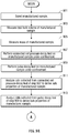
- the testing apparatus and method as described above can be adapted to perform one single experiment that measures the bulk properties (e.g., permeability, porosity, and others) of heterogeneous microporous material as shown in the flow chart of Figures 5A to 5C .
- the bulk properties result from a distribution of the respective properties that are inherently present in the heterogeneous microporous material.
- test sample the sample of heterogeneous microporous material to be tested (i.e., "test sample") is selected.
- the total bulk volume ( V total ) of test sample is measured using a standard water immersion or mercury immersion method. If the test sample has a well-defined shape (e.g., such as a cylindrical plug), direct measurements of dimensions of the test sample can be performed using a vernier caliper, micrometer, or equivalent and the geometric volume of the test sample can be calculated from the measured dimensions. The geometric volume can be used for quality control of the immersion measurement for measuring the total bulk volume of the test sample.
- step 505 the total mass of the test sample before crushing ( M total ) is measured.
- the test sample is crushed by crushing equipment that breaks the test sample, which can initially consist of one or more fragments of arbitrary shape, into smaller fragments.
- the crushing equipment is configured such that the size of the fragments of the test sample produced by the crushing equipment is i) as large as possible and ii) smaller than the largest fragment before crushing so that at least some crushing occurs and sufficiently large fresh surface area is created by crushing.
- Crushing equipment is typically controlled by some kind of aperture parameter, measured in units of length, which is related to the maximum size of produced fragments. This aperture parameter must be set below the minimum of the three dimensions of the largest of the initial fragments. The largest fragment and its dimension can be roughly estimated from a visual inspection of the fragments, using rough measurements with a ruler or vernier caliper.
- step 509 the dimension of the maximum size fragment of the test sample produced by the crushing of step 507, R max , is measured.
- R max the dimension of the maximum size fragment of the test sample produced by the crushing of step 507.
- This can be done by a simplified sieve analysis which isolates the maximum size fragments and relates them to a sieve. Note that the simplified sieve analysis does not measure the masses of the fractions of the fragments that are isolated by the sieve analysis.
- the R max measurement can also be made using digital image analysis of the fragment set or any other suitable method.
- step 511 a pressure test is run on the entire fragment size distribution resulting from the crushing of step 507.
- This pressure test can be executed without flushing.
- the valve control and interface module 133 controls the intermediate valve 107 to assume a closed position in order to isolate the reference cell 101 from the sample cell 103, and the sample cell 103 is loaded with the entire fragment size distribution resulting from the crushing of step 507 and closed at atmospheric pressure.
- Zero or more billets 127 can also be loaded into the sample cell 1 03.
- the set of billets 127 loaded into the cell is selected in such a way that maximizes the total volume of billets in the cell.
- the intake valve 111 is controlled to assume an open position to fluidly couple the source of testing gas 109 (preferably helium) to the reference cell 101 in order to fill the reference cell 101 with testing gas at the predetermined elevated pressure of the test.
- the initial test gas pressure (source pressure P s ) is usually set at the highest possible pressure within the working range of the equipment because this setting provides the maximum amplitude of the pressure signal attributed to pressure diffusion. However, the initial pressure can be set at any pressure within the working pressure range (above 2 atmospheres absolute pressure is recommended), if testing at different gas pressure is required.
- the valve control and interface module 133 controls the intake valve 111 to assume a closed position to isolate the reference cell 101.
- the valve control and interface module 133 controls the intermediate valve 107 to assume an open position for a very short period of time (typically on the order of tens or hundreds of milliseconds), which is sufficient to flow substantial amounts of the testing gas from the reference cell 101 into the sample cell 103. During this flow period, the pressure in the reference cell 101 falls rapidly, due to gas expansion from the reference cell 101 into the free volume of the sample cell 103. Then, the valve control and interface module 133 controls the intermediate valve 107 to assume a closed position that isolates both the reference cell 101 and the sample cell 103. After the intermediate valve 107 is closed, the gas pressure in the sample cell 103 begins to decrease at a slower rate due to diffusion of gas into the porous sample 129.
- the data acquisition module 135 is configured to cooperate with the pressure sensor 117 and the temperature sensor 119 to measure and record the temperature and pressure of the reference cell 101 over time.
- the data acquisition module 135 is also configured to cooperate with the pressure sensor 121 and the temperature sensor 123 to measure and record the temperature and pressure of the sample cell 103 over time.
- the data acquisition module 135 is configured to cooperate with the temperature sensor 125 to measure and record the average temperature of the system over time.
- the data analysis module 137 is configured to extract the data segments corresponding to the pressure decay stage of the test of step 511 and shift the data segments to the same starting time t 0 .
- Time t 0 is dictated by the timestamp value for the time when the pressure of the sample cell 1 01 starts increasing after the intermediate valve 107 has been opened.
- the data analysis module 137 is configured to utilize the results of one or more calibration operations to transform the raw pressure and temperature values of the data segments of the pressure decay stage as generated in step 513 to corrected values that compensate for systematic errors of the apparatus as described herein.
- the data analysis module 137 matches the corrected values of the data segments of the pressure decay stage as generated in step 515 to pressure curves (i.e., pressure data) generated by a computational model of the pressure decay stage with curve-related parameters ⁇ , ⁇ , and ⁇ .
- the computational model of step 517 assumes that all particles have equal size R max as measured in step 509 and that there is a single permeability for all particles.
- the matching identifies the pressure curve that is best-fit to the corrected values of the data segments of the pressure decay stage as generated in step 515.
- the curve-related parameter ⁇ (diffusion relaxation time) for the best-fit pressure curve is then identified for subsequent processing.
- step 519 the data analysis module 137 compares the curve-related parameter ⁇ (diffusion relaxation time) identified in step 517 to the time period time period T decay of the pressure decay stage of the test of step 511 in order to determine whether the maximum particle size is appropriate for the pressure testing of step 527 and subsequent data analysis. For the case where the time period T decay is greater than the curve-related parameter ⁇ (diffusion relaxation time) the operations continue to step 525. For the case where the time period T decay is less than or equal to the curve-related parameter ⁇ (diffusion relaxation time), the operations continue to step 521.
- ⁇ diffusion relaxation relaxation time
- the data analysis module calculates a target maximum particle size R max_target which is less than the particle size R max measured in step 509.
- the target maximum particle size R max_target target is based on the particle size R max measured in step 509, the curve-related parameter ⁇ (diffusion relaxation time) identified in step 517, and the time period time period T decay of the pressure decay stage of the test of step 511.
- step 523 the crushing equipment is configured such that the size of the fragments produced by the crushing equipment is at or near the target maximum particle size R max_target calculated in step 521, and the fragments of the test sample are crushed further by crushing equipment into smaller fragments at or near the target maximum particle size R max_target .
- the operations return to repeat steps 509 to 519 to compare the curve-related parameter ⁇ to the time period time period T decay in order to determine whether the maximum particle size is appropriate for the pressure testing of step 527 and subsequent data analysis. Multiple iterations of the crushing and testing and analysis of steps 511 to 519 can be performed if necessary.
- step 525 sieve analysis is performed to physically separate the fragments of different sizes from one another and to measure the frequency of each respective fragment size within the particle size distribution of the fragments of the test sample produced by the crushing of step 507 and possibly step 523 as needed.
- step 527 a pressure test is run on the entire fragment size distribution resulting from the crushing of step 507 and possibly step 523 as needed.
- the valve control and interface module 133 controls the intermediate valve 107 to assume a closed position in order to isolate the reference cell 101 from the sample cell 103, and the sample cell 103 is loaded with the fragment size distribution at atmospheric pressure.
- Zero or more billets 127 can also be located within the sample cell 103. The set of billets 127 loaded into the sample cell 103 is selected in such a way that the total volume of billets 127 in the sample cell 103 is maximized .
- the valve control and interface module 133 controls the intake valve 111 to assume an open position to fluidly couple the source of testing gas 109 (preferably helium) to the reference cell 101 in order to fill the reference cell 101 with testing gas at an initial elevated (for example, at approximately 1 atmosphere above atmospheric or higher).
- testing gas 109 preferably helium
- Each flushing cycle consists of flowing the testing gas from the reference cell 101 to the sample cell 103, closing the intermediate valve 107, and releasing the gas mixture through the exhaust port 113 to atmosphere by opening and then closing the exhaust valve 115.
- the valve control and interface module 133 controls the intermediate valve 107 to assume a closed position in order to isolate the reference cell 101 from the sample cell 103, and the intake valve 111 is controlled to assume an open position to fluidly couple the source of testing gas 109 to the reference cell 101 in order to fill the reference cell 101 with testing gas at the predetermined elevated pressure of the test. After filling the reference cell 101 with testing gas, the intake valve 111 is controlled to assume a closed position to isolate the reference cell 101.
- the valve control and interface module 133 performs a wait operation for a waiting time of approximately 200-400 seconds in order to allow the temperature in the reference cell 10 1 to equilibrate with the ambient temperature and the sample cell temperature. Equilibration is necessary to make accurate measurements of the initial pressures in the cells.
- the valve control and interface module 133 controls the intermediate valve 107 to assume an open position for a very short period of time (i.e., 0.1 seconds, which is sufficient to flow substantial amounts of the testing gas from the reference cell 101 into the sample cell 103. During this flow period, the pressure in the reference cell 101 falls rapidly, due to gas expansion from the reference cell 101 into the free volume of the sample cell 103.
- the valve control and interface module 133 controls the intermediate valve 107 to assume a closed position that isolates both the reference cell 101 and the sample cell 103. After the intermediate valve 107 is closed, the gas pressure in the sample cell 103 begins to decrease at a slower rate due to diffusion of gas into the porous sample 129. These operations are referred to as the pressure decay stage and continue for the time period T decay .
- the valve control and interface module 133 controls the exhaust valve 115 to assume an open position that fluidly couples the sample cell 103 to the exhaust port 113 at atmosphere for a short period of time (e.g., 1-3 seconds) in order to drop the pressure of the sample cell 103 to atmospheric.
- valve control and interface module 133 controls the exhaust valve 115 to assume a closed position that isolates the sample cell 103.
- the gas pressure in the sample cell 103 increases as gas diffuses out of the porous sample 129 into the interior space of sample cell 103.
- the data acquisition module 135 is configured to cooperate with the pressure sensor 117 and the temperature sensor 119 to measure and record the temperature and pressure of the reference cell 101 over time.
- the data acquisition module 135 is also configured to cooperate with the pressure sensor 121 and the temperature sensor 123 to measure and record the temperature and pressure of the sample cell 103 over time.
- the data acquisition module 135 is configured to cooperate with the temperature sensor 125 to measure and record the average temperature of the system over time.
- the data analysis module 137 is configured to extract the data segments corresponding to a respective pressure decay stage and subsequent degas stage of the pressure test of step 527 and shifts the data segments to the same starting time t 0 .
- Time t 0 is dictated by the timestamp value for the time when the pressure of the sample cell 101 starts increasing after the intermediate valve 107 has been opened.
- the data analysis module 137 is configured to utilize the results of one or more calibration operations to transform the raw pressure and temperature values of the data segments of the pressure decay stage(s) and the pressure degas stage(s) as generated in step 529 to corrected values that compensate for systematic errors of the apparatus as described herein.
- the data analysis module 137 matches the corrected values of the data segments of the pressure decay stage(s) and the pressure degas stage(s) for the pressure test of step 527 to pressure curves (i.e., pressure data) generated by a computational model of the pressure decay stage(s) and pressure degas stage(s) with curve-related parameters ⁇ , ⁇ , and ⁇ .
- the computational model of step 533 assumes the particle size distribution as measured in step 527.
- the matching identifies the pressure curve that is best-fit to the corrected values of the data segments of the pressure decay stage(s) and the pressure degas stage(s) as generated in step 531.
- a minimum set of fixed parameters may be required to calculate the best fit.
- These fixed parameters can include i) the free volumes of the reference cell 101 and the sample cell 103 (i.e., the cell volume subtracting the volume of the billet(s) 127 in the sample cell 103; ii) the initial guess for the bulk sample volume; iii) parameters corresponding to the particle size distribution as measured in step 527; and iv) other necessary parameters for the computational model as needed.
- the values of the curve-related variables (e.g., ⁇ , ⁇ , ⁇ ) of the best-fit curve can be transformed into an estimation of bulk properties of the test sample 129, including bulk volume V sample of the test sample 129, porosity ⁇ of the test sample 129, and permeability k of test sample 129.
- the bulk volume V sample of the test sample 129 can be derived from Eqs. (28) and/or (29).
- the porosity ⁇ of the test sample 129 can be derived from Eqs.
- This porosity, derived from curve matching, can be further referred to as gas-probed porosity or pressure decay matrix porosity ⁇ m
- the permeability k of test sample 129 can be derived from Eq. (32).
- This permeability, derived from curve matching, can be further referred to as gas-probed permeability or matrix pressure decay permeability k m .
- the grain volume V grain of the test sample can be calculated from the bulk volume and the porosity from Eq. (32). Additional properties of the test sample can also be computed as follows.
- step 535 the properties of the sample generated by the analysis of step 533 can be integrated together for visualization and data analysis operations as needed.
- curve-related parameter ⁇ i.e., the diffusion relaxation time
- the permeability resulting from the interpretation of each pressure decay test is averaged through all permeability distributions inside all particle size ranges. Properties estimated from multiple repeats of pressure decay tests can be averaged, and the scatter of the properties estimated from multiple repeats can be utilized to characterise the precision of the measurement.
- the effective gas-filled porosity ⁇ a is greater than the matrix pressure decay porosity ⁇ m , which indicates that only a portion of the initial pore volume in the test sample is visible by gas probing.
- cylinder, cube, drill cuttings if the effective size of the fragments can be estimated. Any size of the fragment that can fit into the sample cell of testing equipment (small dimension less than 1 inch (25.4 mm) most typical) can be used. In case of drill cuttings, which typically have their surface layer contaminated and altered by the invasion of drilling mud, it is important to remove this contaminated layer by either cleaning it chemically or by any other method that allows characterisation of the intact material.
- Another method that maximizes the portion of pore volume visible to gas probing and compensates for these mechanisms is to use different testing gas or liquid. Increasing the pore fluid viscosity by a factor of n will increase the testing time by the same factor, and make a portion of the fastest pore volume visible to the pressure decay probe. This method helps to mitigate the problem of too fast diffusion time or, equivalently, the visible pore volume reduction, but will not help in mitigating the loss of organic porosity due to crushing and removing the organic rich interfaces.
- the downside of this approach is that overall testing time increases by a factor of n.
- the extrapolated permeability attributed to the portion of the pore volume not visible to the gas probe, should be higher than the permeability estimated on the visible portion of pore volume.
- the testing apparatus and methodology as described above can be adapted to perform an experiment that measures the distribution of permeability, porosity, and grain and bulk density in a fragmented material as shown in the flow chart of Figure 6 .
- steps 501 to 523 are performed to ensure the fragmented material has a maximum particle size small enough to perform the pressure decay stage within the defined test time T decay . If one or more of the steps have already been completed, they can be omitted as desired and the processing continues to step 525.
- step 525 sieve analysis is performed to physically separate the fragments of different sizes from one another and to measure the frequency of each respective fragment size within the particle size distribution of the fragments of the test sample produced by the crushing of step 507 and possibly step 523 as needed.
- step 527' the pressure test of step 527 is run for each fraction of the fragment size distribution resulting from the crushing of step 507 and possibly step 523 as needed.
- the details of the pressure test of step 527 are described above.
- step 529' the data extraction and analysis of steps 529 to 533 are performed on the data segments resulting from the pressure decay stage(s) and the pressure degas stage(s) of the pressure test for each fraction of the fragment size distribution.
- the data analysis of step 529' identifies the pressure curve that is best-fit to the corrected values of the data segments of the pressure decay stage(s) and the pressure degas stage(s) of the fraction.
- a minimum set of fixed parameters may be required to calculate the best fit. These fixed parameters can include i) the free volumes of the reference cell 101 and the sample cell 103 (i.e., the cell volume subtracting the volume of the billet(s) 127 in the sample cell 103; ii) the initial guess for the bulk sample volume; iii) parameters corresponding to the particle size of the fraction; and iv) other necessary parameters for the computational model as needed.
- the curve-related variables e.g., ⁇ , ⁇ , ⁇
- sample-related properties including porosity ⁇ and permeability k of the test sample as a function of particle size. Additional properties of the test sample as a function of particle size can also be computed.
- Such additional properties can include the effective gas-filled porosity ⁇ a as a function of particle size, the matrix pressure decay porosity ⁇ m as a function of particle size, the matrix pressure decay permeability k m as a function of particle size, the bulk density ⁇ b as a function of particle size, and the grain density ⁇ g as a function of particle size.
- step 535' the properties of the test sample as a function of particle size as generated by step 529' can be integrated together for visualization and data analysis operations as needed.
- Figures 7A and 7B show an exemplary visualization produced in step 535' for two different heterogeneous rocks, where porosity, permeability, and bulk and grain density are plotted as functions of particle size.
- the visualization in addition to the distribution of porosity and permeability in the test sample, the visualization also shows information about properties of the rock fabric. Bends on the k m ( R s ) and ⁇ m ( R s ) curves indicate that there are some intrinsic length-scales in the natural rock fabric.
- FIGS 8A and 8B An example of the results of the third step is shown in Figures 8A and 8B for two different mudstones A and B. These plots also show the effective gas-filled porosity ⁇ a calculated as the normalized difference of bulk volume and grain volume. The comparison of the maximum cumulative gas-probed porosity and the density-based porosity is indicative of the overall coverage of gas probing.
- the achieved coverage for 'Mudstone A' is about 15% of the pore volume. This is the worst case scenario, which happened because of the weak rock fabric and too low initial crushed particle target size.
- the achieved coverage for 'Mudstone B' is about 65% of the pore volume and is in the normal range.
- the testing apparatus and methodology as described above can be adapted to perform an experiment that measures the distribution of permeability, porosity, and other properties in a manufactured sample as shown in the flow chart of Figures 9A to 9C .
- the manufactured sample has a controlled shape. For example, it can be a cylindrical plug, wafer, or a rectangular slab.
- the manufactured sample is cut or otherwise divided into pieces (e.g., slices of variable thickness) for testing. The pieces may be subsequently crushed into fragmented material for testing of the crushed material.
- the minimum amount of material that can be tested is about 1 inch (25.4 mm) diameter x 2 inch (50.8 mm) long cylindrical plug, which is typically enough to produce from four to seven data points on the length scales varying from 1 to 0.05 inches (25.4 to 1.3 mm).
- the minimum of material should be enough to prepare at least three different sizes of fragments, at least 30 grams of material each.
- the amount of material must be doubled or tripled.
- Other, non-cylindrical shapes can be used as well if used for unconfined pressure decay testing only; however cylindrical shape provides multiple advantages such as convenient size reduction by slicing and the possibility of testing samples under confinement.
- the axes of plugs can be oriented in a predetermined manner during the cutting to provide the minimum variability along their axes.
- samples will be aligned parallel to the horizontal bedding planes.
- the probing of different sizes is predominantly characterising the intrinsic distribution of permeabilities in the sample, which are about proportionally represented in each slice.
- the slicing can be performed parallel to the bedding planes. In this case, the probing of differently sized subsamples is predominantly characterising the spatial distribution of permeabilities in the bedding planes (i.e., the set of rock laminae).
- step 901 the manufactured sample is selected for testing.
- the total bulk volume of the manufactured sample is measured using a standard water immersion or mercury immersion method.
- Direct measurements of dimensions of the test sample can be performed using a vernier caliper, micrometer, or equivalent and the geometric volume of the test sample can be calculated from the measured dimensions.
- the geometric volume can be used for quality control of the immersion measurement for measuring the total bulk volume of the manufactured sample.
- step 905 the mass of the manufactured sample is measured.
- a pressure decay test followed by a pulse decay test are performed on the manufactured sample under confinement using a modified pulse decay test apparatus as shown in Figure 10 .
- This apparatus includes a source of testing gas 1001 (which is a low viscosity chemically inactive gas such as helium or nitrogen) that is fluidly coupled to an upstream reservoir 1005 of volume V 1 , a sample holder 1007 that defines a closed volume that holds the manufactured sample and is capable of applying confining stresses (typically isostatic) to the manufactured sample as dictated by a gas or liquid source 1009 and measured by a pressure sensor P c , and a downstream reservoir 1011 of volume V 2 .
- a pressure transducer P1 measures the absolute pressure of the upstream reservoir 1005.
- a pressure transducer P2 measures the absolute pressure in the downstream reservoir 1011.
- An upstream flow line 1013 with inline valve 1014 is fluidly coupled between the upstream reservoir 1005 and the inlet 1015 of the sample holder 1007.
- a downstream flow line 1017 with an inline valve 1018 is fluidly coupled between the outlet 1019 of the sample holder 1007 and the downstream reservoir 1011.
- a pressure transducer Ps measures the absolute pressure inside the closed volume of the sample holder 1007 that contains the manufactured sample.
- a fill valve 1002 is fluidly coupled to the outlet of the gas source 1001.
- An upstream fill supply line 1021 is fluidly coupled between the fill valve 1002 (and a vent valve 1003 to atmosphere) and the upstream flow line 1013 (upstream of the valve 1014).
- a downstream fill supply line 1023 with inline valve 1004 is fluidly coupled between the fill valve 1002 (and the vent valve 1003) and the downstream flow line 1017 (downstream of the valve 1018).
- the fill valve 1002, vent valve 1003 and valves 1014, 1004, and 1018 are electronically controlled by a test controller similar to the testing apparatus of Figure 2 .
- V 1 is the total upstream volume, which includes the internal volumes of the upstream reservoir 1005, the chamber of the pressure transducer PI, the connecting lines to the pressure transducer P1 and valves 1014, 1004, the fill valve 1002, the vent valve 1003, and the upstream dead volume V du (which is the volume inside valve 1014, the upstream end plug of the sample holder 1007, and the pressure sensor P s ).
- V 2 is the total downstream volume, which includes the internal volumes of the downstream reservoir 1011, the chamber of the pressure transducer P2, the connecting line to valve 1004, and the downstream dead volume V dd (which is the volume inside valve 1018 and the downstream end plug of the sample holder 1007).
- the volumes V 1 , V 2 V du and V dd can be found from calibration using Boyle's Law techniques.
- the pore volume of the manufactured sample is filled with testing gas to a pore pressure typically between 100 and 2,000 psig (7.03 and 140.6 kg/square cm gauge), which is required as an initial condition for the subsequent pulse decay testing.
- Pressure-time data during this filling stage is recorded and then interpreted to estimate bulk properties of the manufactured sample.
- valves 1014, 1004, and 1018 are open, all other valves are closed, pressures recorded by transducers P1 and P2, which are equal through this stage as long as valve 1004 is open, are stabilized and therefore indicate the initial (low) pressure throughout the system and inside the pore volume of the sample.
- valves 1014 and 1018 are closed and valve 1004 remains open.
- the fill valve 1002 is opened to fill both the upstream reservoir 1005 and the downstream reservoir 1011 to a pressure typically equal to or slightly above the target pore pressure for pulse decay testing.
- valves 1014 and 1018 are simultaneously opened and testing gas is allowed to flow from the reservoirs to fill the pore volume of the manufactured sample held within the sample holder 1007.
- the fill period should allow adequate time for the testing gas to diffuse into the (typically) low-permeability manufactured sample.
- the absolute pressure of the upstream and downstream reservoirs 1005 and 1011 is monitored until no further change is observed, indicating thermal and pressure equilibrium.
- the flow regime in this stage is equivalent to the flow regime in the isolated cell pressure decay testing (gas flows from outside of the sample into the pore volume of the sample), except that the volume with elevated initial pressure and low initial pressure are not isolated, but connected throughout the test.
- This test can be referred to as the connected cell pressure decay test.
- the pulse decay test of step 909 is started. At least valves 1014 and 1004 are closed, and the fill valve 1002 is opened to increase pressure in the upstream reservoir 1005 by ⁇ p, which is typically 2 to 20 percent of P 2 [0], and then closed. After the pressure in the upstream reservoir 1005 becomes stable, valve 1014 and valve 1018 are opened to initiate the pressure-transient portion of the test.
- the output of the pressure transducers PI, P2 for the upstream and downstream reservoirs can be monitored as a function of time. Temperature sensors can also be used for measuring temperatures of the upstream reservoir 1005, the downstream reservoir 1011, the closed volume of the sample holder 1007 and ambient temperature as needed similar to the configuration of the testing apparatus of Figure 2 .
- step 911 the data collected from the connected cell pressure decay test of step 907 can be analyzed to measure bulk properties of the manufactured sample under confinement.
- Such properties can include pressure decay porosity, pressure decay permeability, and grain volume of the manufactured sample under confinement.
- the data analysis of step 911 can involve operations similar to the data analysis methodology described above for interpretation of isolated cell pressure decay test results. Specifically, the data analysis can identify the best matching curve-related variables (e.g., ⁇ , ⁇ , ⁇ ) as described above.
- the bulk volume of the manufactured sample, V sample is known from the pre-test measurements and is not identified from the pressure-time data.
- the pressure decay porosity, permeability, and grain volume of the manufactured sample under confinement can be estimated using the same Eqs. (30), (31A), (31B), (32) and (33), where the sample cell volume in the isolated cell pressure decay testing is replaced by a sum of upstream and downstream volume of the modified pulse decay system ( V 1 and V 2 ), plus the volume inside valve 1004.
- the connected cell pressure decay test of step 907 can fill the pore volume to a target pulse decay pore pressure by flowing the testing gas from the upstream side (valves 1014 and 1004 open, valve 1018 closed) or from the downstream side (valves 1018 and 1004 open, valve 1014 closed).
- the upstream (or downstream) pressure decay porosity, upstream (or downstream) pressure decay permeability, and grain volume of the manufactured sample can be estimated using the same Eqs.
- sample cell volume in the isolated cell pressure decay testing is replaced by a sum of upstream volume and downstream dead volume V 1 + V dd minus the volume of valve 1018 for the upstream case (or minus volume of valve 1014 for the downstream case).
- step 913 the data collected from the pulse decay test of step 909 can be analyzed to derive the fabric permeability of the manufactured sample under confinement.
- Fabric permeability which is a result of pulse decay testing that implements flow of gas through the sample from upstream to downstream reservoir, can be different from pressure decay permeability, which is a result of pressure decay testing that implements a different regime of gas flow, which happens from outside of the sample into the pore volume, in the case of heterogeneous samples.
- fabric permeability and pressure decay permeabilities are the same.
- the pressure in the total downstream volume V 2 ( P 2 [ t ]) remains constant for a short period of time until the pressure pulse has traversed the length of the manufactured sample. Then the pressure P 2 [ t ] rises. Because P 1 [ t ] declines and P 2 [ t ] rises, the differential pressure between the upstream and downstream reservoir over time ( ⁇ p [ t ]) continues to diminish and gradually approaches zero as the upstream and downstream pressures become equal. The rate of pressure decay depends on the fabric permeability of the sample, i.e. the lower the permeability the slower the decay.
- the manufactured sample can be cut into multiple thin slices of various thicknesses, using a diamond wire saw, or any other alternative method capable of creating thin parallel slices of the manufactured sample with minimum alteration of the cut surfaces.
- a sample holder can be used and the first slice can be discarded in the event that it is not perfectly parallel.
- step 917 after the amount of sliced material of a given thickness satisfies the minimum material requirements for pressure testing, the sliced material of each given thickness is collected separately for further pressure testing (step 919).
- Steps 915 and 917 can be repeated to collect groups of slices where the slices of each group have a common thickness.
- the thickness of the slice groups can be increased in steps according to a desired length-scale sampling.
- step 919 the slices of a given group (which share a common thickness) are loaded into the sample cell of the testing apparatus of Figure 2 , which is operated to carry out pressure tests without confinement and data analysis operations in the manner described above in order to measure properties of the slices of the group, including porosity and permeability of such slices.
- the common thickness of the slices of the group is used as the characteristic size of the sample in the analysis of the test.
- the pressure testing and data analysis operations of step 919 can be repeated for each group of slices as collected in the operations of steps 915 and 917.
- crushing equipment is configured such that the target size of the fragments produced by the crushing equipment is slightly below the initial thickness of the one or slices, and the slices are crushed by crushing equipment into fragments at the target size.
- step 923 sieve analysis is performed to physically separate the fragments of different sizes from one another and to measure the frequency of each respective fragment size within the particle size distribution of the fragments produced by the crushing of step 921.
- step 925 after the amount of fragmented material of a given size satisfies the minimum material requirements for pressure testing, the fragmented material for the given size is collected separately for further pressure testing (step 927).
- Steps 921 to 925 can be repeated to collect fragmented material of different sizes.
- the sizes of the fragmented material can be increased in steps according to a desired size-scale sampling.
- step 927 the fragments of a given size are loaded into the sample cell of the testing apparatus of Figure 2 , which is operated to carry out pressure testing without confinement and data analysis operations in the manner described above in order to measure properties of the fragments, including sample volume, porosity, and permeability of such fragments.
- the sample bulk volume, porosity, permeability, and sample grain volume of such fragments can be estimated using Eqs. (28), (29), (30), (31A), (31B), (32) and (33) as described above.
- the characteristic size of the fragments is used as the characteristic size of sample in the analysis of the test.
- the pressure testing and data analysis operations of step 927 can be repeated for each given size (fraction) of fractures collected in the repeated operations of steps 921 and 925.
- the pressure testing and data analysis operations of step 927 allows for computation of properties of the manufactured sample as a function of fragment (particle) size, including porosity ⁇ and permeability k of the manufactured sample as a function of fragment (particle) size. Additional properties of the test sample as a function of particle size can also be computed. Such additional properties can include the effective gas-filled porosity ⁇ a as a function of particle size, the matrix pressure decay storage ⁇ m as a function of particle size, the matrix pressure decay permeability k m as a function of particle size, the bulk density ⁇ b as a function of particle size, and the grain density ⁇ g as a function of particle size.
- step 929 the properties of the confined manufactured sample and slices resulting from the pressure decay test and the pulse decay test of steps 907 and 909, respectively, as well as the properties of the unconfined slices and crushed fragments resulting from the pressure tests of steps 919 and 927 can be integrated together and analyzed to identify a multiple-porosity and multiple-permeability computational material model that describes porosity and permeability of all subsamples of the material obtained by controlled size reduction and by crushing into fragments.
- Multiple-porosity multiple-permeability model assumes that total porosity of the material is subdivided into two to n pore subsystems.
- Each of the pore subsystems is characterised by its own porosity; sum of the porosities of all subsystems is equal to the total porosity.
- Each of the pore systems is characterised by its own permeability; value of permeability is decreasing with the index of the pore system.
- Pore systems can be connected with each other in various ways; interaction between pore systems is defined by connectivity parameters.
- the computational model is identified as the computational material model with a minimum number of parameters that successfully fits the measurements for all sizes of slices and samples and assumes that all parameters such as porosities, permeabilities, and connectivities of pore subsystems, are uniformly distributed throughout the manufactured sample, i.e. does not depend on space coordinates.
- the model can be used in the commercial fluid flow simulators such as ECLIPSE, available from Schlumberger Technology Corporation of Sugar Land, Texas, USA, or others to predict fluid flow at different scales, using simulated domains of different size and geometry, using different flow regimes and boundary conditions.
- ECLIPSE commercial fluid flow simulators
- step 929 the properties of the manufactured sample as a function of particle size as generated in step 919 (properties of slices derived by controlled size reduction) and in step 929 (properties of fragments derived by crushing) can be integrated together for visualization and data analysis operations as needed.
- Controlled size reduction is not sensitive to the presence of strength fabric in the sample, and only reveals length scales of permeability fabric.
- Permeability distribution on the crushed fragments is sensitive to both permeability and to the rock strength fabric. Comparison of the two distributions indicates if the permeability and strength fabric are overlapping or are independent from each other in the initial sample.
- the permeability distribution of the crushed fragments also gives more details on the fine scale variability of the low-end matrix permeability of the sample and on the breakdown of this low-end permeability distribution in relation to the pore volume and the bulk volume of the initial sample.
- Figure 11 shows an example of properties of unconfined material measured by the pressure testing and data analysis operations of step 919 on groups of slices with different thickness as cut from an exemplary manufactured sample (in this case, a cylindrical plug of Mudstone C). Note that due to the presence of highly conductive network connecting low permeability matrix elements (which are much smaller than characteristic size of the slices), the measured permeability of the slice groups grows with slice thickness.
- steps 915 to 919 can be adapted to test other controlled shapes of material in the manner similar to the slices as described above.
- the measurements and analyses of the connected cell pressure decay test of step 907 and the pulse decay test of step 909 can be carried out at different levels of confinement stress (by varying the pressure of the gas source 1009) in order to evaluate the sensitivity of the measured properties to varying confinement stress.
- the measurements and analyses of the connected cell pressure decay test of step 907, the pulse decay test of step 909, and the unconfined pressure tests of steps 919 and 927 can be carried out at different pore pressures in order to evaluate the sensitivity of the measured properties to varying pore pressure (particularly for the dependence of apparent permeability related to Knudsen flow regimes).
- the measurements and analyses of the connected cell pressure decay test of step 907, the pulse decay test of step 909, and the unconfined pressure test of steps 919 and 927 can be carried out using different testing gases or liquid in order to characterise pore throat sizes, molecular sieving, adsorption, and wettability effects.
- the manufactured sample as described above can be prepared by covering one or more selected surfaces (or selected parts of the surfaces) of the samples by an impermeable material (such as epoxy or other suitable material) in order to selectively seal some of the flow directions to measure permeabilities in different directions, such as azimuthal permeability measurements along the bedding planes or transverse measurements perpendicular to the bedding planes.
- an impermeable material such as epoxy or other suitable material
- Another usage of the selective coating of the surfaces of the sample is to minimize the dead volume in the sample cell to increase signal-to-noise ratio.
- the coating has to be sufficiently thick, have accurately measured volume, and closely repeat the internal surface of the testing cell, providing both minimum gap between the coated sample and the internal surface of the cell and allowing for easy loading and unloading of the sample.
- step 907 can be omitted.
- Natural microporous materials can be extremely heterogeneous and may have a quite complex spectrum of pore sizes and shapes, which can result in apparent permeability behavior that can be unique for different types of materials and different from both Eqs. (46) and (47). Therefore it requires direct measurement of apparent permeability as function of gas pressure.
- Measuring the apparent permeability of a microporous sample can be carried out with the isolated cell pressure decay apparatus of Figure 2 in conjunction with the operations illustrated in flowchart of Figures 13A and 13B .
- the microporous sample is loaded into the sample cell of the apparatus of Figure 2 .
- One or more billets 127 may be added into the sample cell in order to minimize dead volume.
- step 1303 a sequence of pressure decay tests at different initial pressures is performed and the results recorded by the apparatus. This can be done using scripts similar to ascending and descending 'sweep 1' and 'sweep 2' used for calibration of system volumes, pressure transducer non-linearity, and volume compressibilities at different pressures.
- the number of tests in each of the sweeps may need to be decreased in order to increase the initial pressure difference between the reference and sample cells before each of the pressure decay tests to as few as three tests at different pressures in the working pressure range of the system.
- step 1305 data analysis operations are performed that interpret the pressure decay curves that result from the pressure decay tests of step 1303 independently, by fitting each pressure decay curve individually to a proxy model (which, for example, can be based on Eq. (22) as described above) with constant gas compressibility and pressure-independent compressibility.
- This proxy model is fast to compute and allows fully automatic fitting. Since every pressure decay test is run at a different pressure and the curves are interpreted independently, extracted values of apparent permeability k 2i ( P i ) will change with pressure. Note, that flow conditions in the pressure decay test are quite different from steady state flow through cylindrical plugs. In the case of flow through the plug, the pressure difference across the sample is small compared to mean pressure levels, and the pressure-dependent permeability is almost constant throughout the sample.
- step 1307 data analysis is performed to calculate the parameters of the Klinkenberg permeability correction model defined by Eq. (46) that is best-fit to the experimental curve k 2i ( P i ) derived from step 1305.
- Such analysis can derive the parameters k 0 and b of the best fit curve.
- step 1309 data analysis operations are performed that interpret the pressure decay curves that result from the pressure decay tests of step 1303 by fitting the pressure decay curves to a computational pressure decay model with variable gas compressibility and Klinkenberg permeability correction defined by Eq. (46).
- This model is computationally inexpensive.
- the Klinkenberg permeability correction can be based on the parameters k 0 and b derived from step 1307 or from step 1311. Such analysis derives the improved pressure-dependent permeability values k 3i ( P i ) .
- step 1311 data analysis is performed to calculate the parameters of the Klinkenberg permeability correction model defined by Eq. (46) that is best-fit to the experimental curve k 3i ( P i ) derived from step 1309.
- Such analysis can derive new improved parameters k 0 and b for the best-fit curve.
- steps 1309 and 1311 can be repeated over multiple iterations until the results converge.
- the criteria for convergeance can be based on the change in the experimental curve k 3i ( P i ) derived in step 1309 (or the parameters k 0 and b derived in step 1311) satisfying a predetermined threshold for consistency.
- the parameters k 0 and b as derived in step 1309 are defined by a self-consistent set of values k 3i ( P i ).
- the parameters k 0 and b as derived in step 1309 are used as part of the analytical function, denoted k 4 ( P ), that describes pressure dependent permeability and the operations can continue to step 1315. Otherwise, the operations can continue to step 1313 for further improvement of pressure-dependent permeability approximation.
- step 1313 data analysis operations can be performed that fit the function k 4 ( P ) to approximate all values k 3i ( P i ) derived from previous steps.
- Function k 4 ( P ) can be defined by Eq. (47), or any other analytical model of permeability dependence on pressure, or, k 4 ( P ) can be a smooth piece-wise spline interpolation of k 3i ( P i ).
- Further data analysis operations can be performed that simulate the experimental pressure decay curves utilizing the function k 4 ( P ) in conjunction with the models of Eqs. (22)-(24) that allow for arbitrary dependence of permeability on pressure. This model is computationally expensive.
- the differences between the simulated pressure decay curves and the measured pressure decay curves are measured to determine if the results converge.
- the criteria for convergeance can be based on whether a desired quality of match between the simulated pressure decay curves and the measured pressure decay curves has been obtained. If not, the function k 4 ( P ) can be updated and the operations of step 1313 repeated until the desired quality of match is obtained. In the event that the desired quality of match is obtained, the operations can continue to step 1315 for additional analysis.
- step 1315 one or more additional experiments can be performed to characterise properties of the microporous sample. Examples of such additional experiments are described below with respect to Figures 14-17 .
- the operations end after completing step 1315.
- steps 1305 to 1313 perform two loops of fit improvement.
- the first loop iteratively improves the parameters ko and b and uses the Klinkenberg pressure dependence of Eq. (46) only, because the computational model to generate pressure-time curves in this case is fast.
- the second loop uses the best fit from the first loop to start iterative improvement of arbitrary user defined function k 4 ( P ), which has to use computationally expensive calculation of pressure curves.
- the second loop is terminated if the match is already good.
- the pressure decay measurements can be influenced by the slip effect of testing gas.
- the layer of molecules adjacent to and contacting the solid walls of the pores of the sample is stationary.
- the velocity profile of the liquid is maximum at the center of the passageway and zero at the walls.
- the gas velocity profile is not zero at the walls, but has a finite velocity in the direction of flow.
- Gas molecules are in constant motion, colliding with one another after traveling an average distance equal to the "mean free path.” At lower pressures, the mean free path is greater, and the distance between molecular collisions is increased. Internal resistance to flow is provided by gas molecular collisions with the walls.
- helium As was discussed earlier, the most suitable gas to estimate ultra-low permeability is helium, which has the lowest specific heat capacity and the highest thermal diffusivity. This results in the smallest amplitude and shortest time thermal effects that contaminate pressure diffusion measurements. Also helium has a very small molecule size that allows the testing gas to reach the smallest pores, and it is inert gas, which is not chemically interacting with any other species and therefore is not adsorbing inside of any samples. At the same time, there are additional pieces of information about the microporous sample that can be extracted by pressure decay testing of the same material with different gases.
- Figure 14 is a flow chart that illustrates additional experiments that can be carried out using the apparatus of Figure 2 to characterise permeability of the microporous sample in a manner that accounts for such slip effect.
- the additional experiments employ a number of different testing gases.
- the number of different testing gases is preferably realized from monoatomic gases (first preference), diatomic gases (second preference) or combinations thereof.
- step 1401 a series of calibration tests is performed using the apparatus of Figure 2 for various combinations of billet sets 127 in the sample cell 1 03 and at various pressures using each one of the different testing gases in order to quantify early-time thermal effects as a function of volume ratio, pressure and kind of gas.
- step 1403 a series of pressure dependent permeability measurements is performed using each one of the different testing gases.
- the permeability measurements of the series employ the testing apparatus of Figure 2 , which is operated to carry out pressure tests without confinement and data analysis operations in the manner described above in order to measure properties of the microporous sample, including permeability of the sample.
- step 1405 the results of the permeability measurements of step 1403 are combined by translating all permeabilities for all gases to the equivalent permeability of the gas with the largest free mean path (typically helium), using Eq. (50). The combined results can be used to characterise a single dependence of permeability on pressure or free mean molecule path.
- the equivalent permeability of the gas with the largest free mean path typically helium
- additional experiments can be performed to characterise adsorption of the microporous sample.
- the additional experiments employ a testing gas that is non-adsorptive with respect to the microporous sample along with a testing gas that is adsorptive with respect to the microporous sample (such as methane for organic rich reservoir rock).
- the adsorptive characteristics of microporous samples can be estimated by doing isolated-cell pressure decay testing on the same sample using the adsorptive and non-adsorptive testing gases and then comparing the results.
- FIG 15 is a flow chart illustrating operations that characterise adsorption of a microporous sample employing pressure decay testing.
- a permeability measurement of a microporous sample is performed using the testing gas that is non-adsorptive with respect to the microporous sample.
- the permeability measurement employs the testing apparatus of Figure 2 , which is operated to carry out a pressure test without confinement and data analysis operations in the manner described above in order to measure properties of the microporous sample, including permeability of the sample. It is assumed that early-time thermal effect for the non-adsorptive testing gas is known.
- a permeability measurement of a microporous sample is performed using the testing gas that is adsorptive with respect to the microporous sample.
- the permeability measurement employs the testing apparatus of Figure 2 , which is operated to carry out a pressure test without confinement and data analysis operations in the manner described above in order to measure properties of the microporous sample, including permeability of the sample. It is assumed that early-time thermal effect for the adsorptive testing gas is known.
- step 1505 the results of the permeability measurements of steps 1501 and 1503 can be compared and analyzed in order to characterise adsorption of the microporous sample. Specifically, if some amount of the adsorptive testing gas is actually adsorbed, that gas is not contributing to gas pressure in the pore volume and the sample cell and therefore estimated gas-probed porosity is increased. The amount of adsorbed gas is estimated from the difference in measured gas-probed porosity. If gas slip in the sample or pressure dependence of permeability is well established, it is possible to extrapolate what would be the permeability of the sample for the gas which has the same viscosity and molar mass as the adsorptive gas. By comparing the extrapolated permeability for equivalent non-adsorptive gas and the permeability measured with corresponding adsorptive gas it is possible to estimate the adsorption rate of the microporous sample.
- thermal effects due to adiabatic expansion and compression of the testing gas can be highly variable depending on the type of testing gas used.
- the thermal effect can be as short as 2-5 seconds depending on testing conditions.
- thermal effects can be tens of seconds long, which may be comparable to total gas diffusion time in many samples.
- Such thermal effects can make permeability measurement with the heavier gas alone impossible.
- the prolonged period of thermal dissipation recorded on the pressure signal carries more information about the thermal properties of the sample in the cell.
- the thermal properties of a microporous sample can be estimated by doing isolated-cell pressure decay testing on the same sample using helium and a heavier testing gas.
- FIG 16 is a flow chart illustrating operations that characterise thermal properties of a microporous rock sample employing pressure decay testing.
- step 1601 an isolated pressure decay testing at multiple pressures is performed on a microporous rock sample using helium as the testing gas.
- the pressure decay test employs the testing apparatus of Figure 2 , which is operated to carry out a pressure test without confinement using helium as the testing gas. It is assumed that early-time thermal effect for the helium testing gas is known.
- step 1603 an isolated cell pressure decay test is performed on the microporous rock sample using a heavier testing gas that produces a long thermal effect.
- the pressure decay test employs the testing apparatus of Figure 2 , which is operated to carry out a pressure test without confinement using the heavier testing gas. It is assumed that early-time thermal effect for the heavier testing gas is known. Note that the pressure decay measurements of step 1603 combine both thermal effect and gas diffusion.
- step 1605 data analysis operations are performed that process the results of the pressure decay testing at multiple pressures of step 1601 to measure grain volume, grain density, porosity, and pressure dependent permeability of the microporous rock sample for the case where helium is the testing gas.
- the sample volume, porosity, permeability, and grain volume of such fragments can be estimated using Eqs. (28), (29), (30), (31A), (31B), (32), and (33) as described above.
- the function, approximating experimental pressure dependent permeability of the sample, k He ( P ) can be obtained using operations similar to those described above with respect to Figures 13A and 13B .
- step 1607 data analysis is performed that uses the results of step 1605 to estimate equivalent permeability of the heavier gas for the microporous rock sample at the pressures corresponding to the pressure decay test of step 1603 that utilized the heavier testing gas.
- step 1609 data analysis is performed that uses the equivalent permeability of the microporous rock sample for the heavier gas estimated in step 1607 to generate the equivalent pressure decay curve without thermal effects for the case where the heavier testing gas is used.
- the deconvoluted temperature signal T T (t) from step 1611 is further processed to estimate thermal properties of the microporous sample.
- the thermal properties can be derived from a forward numerical model of temperature dissipation in the sample cell enclosing the sample and billets that is used to solve the inverse problem.
- the model takes as an input all essential thermal properties of the sample cell (geometry, thermal conductivity and thermal capacity of cell walls), of the testing gas (mole amount, thermal conductivity and capacity) and billets (billet set, geometry, thermal conductivity and capacity of all billets).
- the initial condition for the model is defined by the initial amount of heat stored in the gas, which is estimated from initial temperature T T (t), and the amount and heat capacity of the testing gas.
- multiple simulation of the model are performed with varied thermal conductivity and thermal capacity of the microporous sample until the best match between the modeled T T (t) and deconvoluted T T (t) from step 1611 is found.
- the thermal properties of the sample can be derived from a full calibrated forward numerical model of the isolated pressure decay equipment interacting with the microporous sample that is used to solve the inverse problem.
- the model takes as an input all essential properties of the testing equipment (volumes, thermal properties and geometry of cells), all essential testing conditions (initial pressures, billet set, thermal properties of billets, gas properties) and properties of the tested material (grain volume, porosity, pressure dependent permeability, which are known from the testing with helium, size and geometry of fragments and thermal properties of the material). All listed inputs except thermal properties of the material are fixed. Then, multiple simulations of the model are performed with varied thermal properties of the material until the best match with experimental curves which carry considerable thermal effect is found.
- the isolated pressure decay testing as described herein can be extended to measure saturation dependent permeability of a microporous sample.
- Relative permeability curves that specify how permeability of specific phases changes as a function of phase saturation is a key input for the simulation and understanding of the multiphase flow in porous rock. For example, in heterogeneous rocks with very fine porosity such as reservoir shales, direct measurement of relative permeability is not practical because of the extremely low mobility of the liquid phase. An important piece of information that helps to understand relative permeability is to identify permeability to gas, which is more mobile, as a function of the saturation by the less permeable liquid phase.
- Isolated cell pressure decay testing on fragmented or controlled shape samples of small size is a suitable method to characterise this dependence, because of its high sensitivity to permeability variations in the low permeability range and because it takes a reasonably short amount of time to diffuse desired liquids into samples to create necessary saturation levels.
- Figure 17 is a flow chart illustrating operations that characterise saturation dependent permeability of a microporous sample.
- small size fragmented samples or controlled shape samples
- the amount of such samples is selected to provide samples to estimate permeability at all desired saturation levels.
- the size of the samples is dictated by the expected or estimated highest (unsaturated) permeability of the sample, which must be within the measurable permeability range at the selected size.
- step 1703 the samples are split into equivalent subsamples, one subsample per desired saturation level.
- controlled saturation levels by one or more desired liquids are created for each subsample.
- the controlled saturation levels of the desired liquid(s) can be attained by controlled evaporation or solvent extraction of the fully saturated subsample.
- step 1707 a pressure decay test is performed on each subsample at the corresponding controlled saturation level created in step 1705.
- the pressure decay test employs the testing apparatus of Figure 2 , which is operated to carry out a pressure decay test without confinement on each subsample at the controlled saturation levels created in step 1705.
- the operations can be performed at different pore pressures as described above.
- step 1709 the results of the pressure tests of step 1707 are processed to measure grain volume, grain density, porosity, and pressure dependent permeability of the microporous rock sample for the different controlled saturation levels of the subsamples.
- the sample volume, porosity, permeability, and grain volume of such fragments can be estimated using Eqs. (28), (29), (30), (31A), (31B), (32), and (33) as described above.
- step 1711 the results of step 1709 can be analyzed to characterise the dependence of permeability (and, optionally, gas slip) on the saturation by different liquids. This is done via comparing and understanding how the permeability and gas slip described by Klinkenberg parameters or by pressure dependent permeability k 4 (P) change with different saturation levels.
- the pressure decay testing at different pressures described in Figures 13A and 13B ; the pressure decay testing with different gases and pressure described in Figure 14 ; the pressure decay testing to characterise adsorptive properties of the rock described in Figure 15 ; pressure decay testing with different saturation levels described in Figure 17 can also be done using the experimental apparatus of Figure 10 under various confinement, if required by a testing program.
- This testing requires cylindrical rock samples, (samples of other shapes can be embedded into machinable impermeable matrix around them, which is then machined to create cylindrical shape of the composite sample). For the same type of microporous material, this testing also takes a longer time than unconfined pressure decay testing, which can use samples of smaller size.
Landscapes
- Chemical & Material Sciences (AREA)
- Life Sciences & Earth Sciences (AREA)
- Health & Medical Sciences (AREA)
- Physics & Mathematics (AREA)
- Immunology (AREA)
- Analytical Chemistry (AREA)
- Pathology (AREA)
- General Physics & Mathematics (AREA)
- General Health & Medical Sciences (AREA)
- Biochemistry (AREA)
- Dispersion Chemistry (AREA)
- Engineering & Computer Science (AREA)
- Environmental & Geological Engineering (AREA)
- Medicinal Chemistry (AREA)
- Food Science & Technology (AREA)
- General Life Sciences & Earth Sciences (AREA)
- Geology (AREA)
- Remote Sensing (AREA)
- Fluid Mechanics (AREA)
- Investigating Strength Of Materials By Application Of Mechanical Stress (AREA)
- Investigation Of Foundation Soil And Reinforcement Of Foundation Soil By Compacting Or Drainage (AREA)
- Manufacture Of Porous Articles, And Recovery And Treatment Of Waste Products (AREA)
- Sampling And Sample Adjustment (AREA)
Claims (11)
- Verfahren zum Charakterisieren von Eigenschaften einer hergestellten Gesteinsprobe, das umfasst:a) Bereitstellen einer ersten Untersuchungsvorrichtung mit einem Probenhalter und zugeordneten vorgelagerten und nachgelagerten Speichern, denen jeweils wenigstens ein Drucksensor zugeordnet ist, wobei der Probenhalter dazu ausgelegt ist, die hergestellte Gesteinsprobe unter druckbeaufschlagter Einschließung zu enthalten, und es gestattet, dass ein Untersuchungsfluidpuls durch die innerhalb des Probenhalters enthaltene hergestellte Gesteinsprobe strömt, und wobei die Drucksensoren der ersten Untersuchungsvorrichtung dazu ausgelegt sind, Druck der vorgelagerten und nachgelagerten Speicher zu messen, während der Untersuchungsfluidpuls durch die innerhalb des Probenhalters enthaltene hergestellte Gesteinsprobe strömt;b) Verwenden der ersten Untersuchungsvorrichtung mit der in den Probenhalter geladenen hergestellten Gesteinsprobe, um Bulk-Eigenschaften der hergestellten Gesteinsprobe zu charakterisieren, gekennzeichnet durchc) Teilen der hergestellten Gesteinsprobe in mehrere Stücke unterschiedlicher Größe;d) Aufteilen der aus c) resultierenden Stücke der hergestellten Gesteinsprobe in Größengruppen unterschiedlicher Größe;e) Durchführen einer Sequenz von Vorgängen für jede gegebene Größengruppe der aus d) resultierenden Stücke, wobei die Sequenz von Vorgängen von e) beinhaltete1) Laden des einen oder der mehreren Stücke der gegebenen Größengruppe in den Probenhalter,e2) im Anschluss an e1), Konfigurieren der ersten Untersuchungsvorrichtung zur Durchführung einer Sequenz von Untersuchungsvorgängen, wobei der beladene Probenhalter mit druckbeaufschlagtem Untersuchungsfluid befüllt und von anderen Teilen der Untersuchungsvorrichtung isoliert wird, und die Drucksensoren zum Messen und Speichern von Druckdaten verwendet werden, die Drücke repräsentieren, die vom Drucksensor im Zeitablauf gemessen werden,e3) Verwenden eines Datenverarbeitungssystems, um die in e2) erzeugten und gespeicherten Druckdaten in Verbindung mit einem Rechenmodell zu verarbeiten, das einen Satz von Druckkurven mit mehreren kurvenbezogenen Variablen und zugeordneten Werten beinhaltet, um eine übereinstimmende Druckkurve zu identifizieren, unde4) Verwenden des Datenverarbeitungssystems zum Verarbeiten der Werte der kurvenbezogenen Variablen für die in e3) identifizierte übereinstimmende Druckkurve, um Eigenschaften der gegebenen Größengruppe von Stücken abzuleiten.
- Verfahren gemäß Anspruch 1, das ferner umfasst, in b) und e4) abgeleitete Eigenschaften der hergestellten Gesteinsprobe darzustellen, um die kombinierten Eigenschaften der hergestellten Gesteinsprobe für einen Nutzer zu visualisieren.
- Verfahren gemäß Anspruch 1, wobei die in b) abgeleiteten Bulk-Eigenschaften der hergestellten Gesteinsprobe ausgewählt sind aus der Gruppe bestehend aus Bulk-Volumen, Bulk-Dichte, Porosität, Permeabilität, Kornvolumen, Korndichte und effektiver dichtebasierter Porosität.
- Verfahren gemäß Anspruch 1, wobei das Rechenmodell auf einer analytischen Abklingfunktion basiert, die drei Parameter, α, β und τ, umfasst, wobei es sich bei dem Parameter α um einen Speicherkoeffizienten handelt, der das Verhältnis von Porenvolumen zu Totvolumen in der zu untersuchenden Probe definiert, der Parameter β sich auf den Enddruck in der Probenzelle, wenn sich der Druck innerhalb und außerhalb des Porenvolumens der zu untersuchenden Probe stabilisiert hat, bezieht, und es sich bei dem Parameter τ um eine Entspannungszeit handelt.
- Verfahren gemäß Anspruch 4, wobei die in e4) abgeleiteten Eigenschaften der gegebenen Größengruppe von Stücken der hergestellten Gesteinsprobe ausgewählt sind aus der Gruppe bestehend aus Bulk-Volumen basierend auf dem Wert des Parameters β für die übereinstimmende Druckkurve, Porosität basierend auf dem Wert des Parameters a für die übereinstimmende Druckkurve, Permeabilität basierend auf dem Parameter τ für die übereinstimmende Druckkurve, Kornvolumen basierend auf dem Bulk-Volumen und der Porosität, Bulk-Dichte basierend auf Bulk-Volumen, Korndichte basierend auf Kornvolumen, und effektiver dichtebasierter Porosität basierend auf Bulk- und Korndichte.
- Verfahren gemäß Anspruch 1, wobei das Verarbeiten von e3) berichtigte Druckwerte basierend auf den als Ergebnis der in e2) erzeugten und gespeicherten Druckdaten ableitet, und die berichtigten Druckwerte mit dem Satz von aus dem Rechenmodell abgeleiteten Druckkurven abgleicht, um die übereinstimmende Druckkurve zu identifizieren.
- Verfahren gemäß Anspruch 1, wobei es sich bei den aus c) resultierenden Stücken um Bruchstücke ungeregelter Form mit Größen, die dem Radius solcher Fragmente entsprechen, handelt.
- Verfahren gemäß Anspruch 1, wobei die aus c) resultierenden Stücke eine geregelte Form mit Größen aufweisen, die der Dicke der geregelten Form entsprechen.
- Verfahren gemäß Anspruch 8, wobei die Stücke mit geregelter Form Scheiben einer Kernprobe mit variierender Dicke sind.
- Verfahren gemäß Anspruch 1, wobei die hergestellte Gesteinsprobe eine aus einer geologischen Formation gewonnene Kernprobe umfasst.
- Verfahren gemäß Anspruch 1, wobei die in b) abgeleiteten Bulk-Eigenschaften der hergestellten Gesteinsprobe eine Gefügepermeabilität kf basierend auf einer Gleichung der Form
 wobei µ die Viskosität des Untersuchungsfluids ist,C die Kompressibilität des Untersuchungsfluids ist,L die Länge der Probe entlang der Untersuchungsfluidströmungsrichtung ist,A die Querschnittsfläche der Probe senkrecht zur Untersuchungsfluidströmungsrichtung ist,V1 und V2 vorgelagerte und nachgelagerte Volumen sind,
 θ1 die erste Wurzel der Gleichung

 Vp das Porenvolumen der hergestellten Gesteinsprobe ist, V = φ · A · L, φ die Porosität der hergestellten Gesteinsprobe ist, und Steilheit die Steilheit der linearen Regression zum linearen Teil der experimentellen Kurve, die durch den Logarithmus des in b) gemessenen differentiellen Pulsabklingdrucks gesteuert wird, ist.
Applications Claiming Priority (2)
| Application Number | Priority Date | Filing Date | Title |
|---|---|---|---|
| US201361762617P | 2013-02-08 | 2013-02-08 | |
| PCT/US2014/014825 WO2014123973A1 (en) | 2013-02-08 | 2014-02-05 | Apparatus and methodology for measuring properties of microporous material at multiple scales |
Publications (3)
| Publication Number | Publication Date |
|---|---|
| EP2954308A1 EP2954308A1 (de) | 2015-12-16 |
| EP2954308A4 EP2954308A4 (de) | 2016-02-10 |
| EP2954308B1 true EP2954308B1 (de) | 2019-05-22 |
Family
ID=51300102
Family Applications (5)
| Application Number | Title | Priority Date | Filing Date |
|---|---|---|---|
| EP15180437.4A Withdrawn EP2977742A1 (de) | 2013-02-08 | 2014-02-05 | Verfahren zur messung der eigenschaften von mikroporösem material in mehreren massstäben |
| EP14749191.4A Active EP2954308B1 (de) | 2013-02-08 | 2014-02-05 | Verfahren zur messung der eigenschaften von mikroporösem material in mehreren massstäben |
| EP14748895.1A Active EP2954307B1 (de) | 2013-02-08 | 2014-02-05 | Verfahren zur messung der eigenschaften von mikroporösem material in mehreren massstäben |
| EP14749295.3A Withdrawn EP2954305A4 (de) | 2013-02-08 | 2014-02-05 | Vorrichtung und verfahren zur messung der eigenschaften von mikroporösem material in mehreren massstäben |
| EP14748832.4A Withdrawn EP2954306A4 (de) | 2013-02-08 | 2014-02-05 | Vorrichtung und verfahren zur messung der eigenschaften von mikroporösem material in mehreren massstäben |
Family Applications Before (1)
| Application Number | Title | Priority Date | Filing Date |
|---|---|---|---|
| EP15180437.4A Withdrawn EP2977742A1 (de) | 2013-02-08 | 2014-02-05 | Verfahren zur messung der eigenschaften von mikroporösem material in mehreren massstäben |
Family Applications After (3)
| Application Number | Title | Priority Date | Filing Date |
|---|---|---|---|
| EP14748895.1A Active EP2954307B1 (de) | 2013-02-08 | 2014-02-05 | Verfahren zur messung der eigenschaften von mikroporösem material in mehreren massstäben |
| EP14749295.3A Withdrawn EP2954305A4 (de) | 2013-02-08 | 2014-02-05 | Vorrichtung und verfahren zur messung der eigenschaften von mikroporösem material in mehreren massstäben |
| EP14748832.4A Withdrawn EP2954306A4 (de) | 2013-02-08 | 2014-02-05 | Vorrichtung und verfahren zur messung der eigenschaften von mikroporösem material in mehreren massstäben |
Country Status (4)
| Country | Link |
|---|---|
| US (5) | US9709478B2 (de) |
| EP (5) | EP2977742A1 (de) |
| CA (5) | CA2890818C (de) |
| WO (4) | WO2014123973A1 (de) |
Families Citing this family (75)
| Publication number | Priority date | Publication date | Assignee | Title |
|---|---|---|---|---|
| CA2890818C (en) | 2013-02-08 | 2023-03-14 | Schlumberger Canada Limited | Apparatus and methodology for measuring properties of microporous material at multiple scales |
| DE102013216450A1 (de) * | 2013-08-20 | 2015-02-26 | Inficon Gmbh | Pico-Prüfleck |
| US10174613B2 (en) * | 2014-01-14 | 2019-01-08 | Halliburton Energy Services, Inc. | Effective porosity determination for tight gas formations |
| US10288517B2 (en) | 2014-04-14 | 2019-05-14 | Schlumberger Technology Corporation | Apparatus and calibration method for measurement of ultra-low permeability and porosity |
| US10274411B2 (en) | 2014-04-14 | 2019-04-30 | Schlumberger Technology Corporation | Methods for measurement of ultra-low permeability and porosity |
| US10061061B2 (en) * | 2014-07-28 | 2018-08-28 | Schlumberger Technology Corporation | Well treatment with digital core analysis |
| CA2960134A1 (en) * | 2014-10-14 | 2016-04-21 | Landmark Graphics Corporation | Using representative elemental volume to determine subset volume in an area of interest earth model |
| DE102015203552A1 (de) * | 2015-02-27 | 2016-09-01 | Robert Bosch Gmbh | Anordnung und Verfahren zur Dichtheitsüberprüfung eines Behältnisses |
| US10156507B2 (en) | 2015-04-01 | 2018-12-18 | Schlumberger Technology Corporation | Determination of free volume of a rock sample using high pressure adsorption data |
| AR104396A1 (es) | 2015-04-24 | 2017-07-19 | W D Von Gonten Laboratories Llc | Posicionamiento lateral y diseño de completamiento para un desempeño mejorado de pozo de reservorios no convencionales |
| US10365202B2 (en) * | 2015-05-11 | 2019-07-30 | Schlumberger Technology Corporation | Method for measurement of ultra-low permeability and porosity by accounting for adsorption |
| CN105004395B (zh) * | 2015-06-08 | 2019-03-12 | 深圳麦开网络技术有限公司 | 一种基于压力感应的容器内液体体积测量装置、容器与方法 |
| CA2989442C (en) * | 2015-07-17 | 2021-06-08 | Saudi Arabian Oil Company | Methods for analyzing natural gas flow in subterranean reservoirs |
| US10591399B2 (en) * | 2015-07-17 | 2020-03-17 | Saudi Arabian Oil Company | Methods for analyzing natural gas flow in subterranean reservoirs |
| EP3391025B1 (de) | 2015-12-14 | 2021-02-17 | Saudi Arabian Oil Company | Verfahren und vorrichtung zur bestimmung des gaspermeabilitäts einer unterirdischen formation |
| US10416064B2 (en) | 2015-12-14 | 2019-09-17 | Saudi Arabian Oil Company | Methods and systems for determining gas permeability of a subsurface formation |
| CN105547959B (zh) * | 2015-12-30 | 2019-01-18 | 中国石油天然气股份有限公司 | 致密基岩中基质孔隙储集天然气能力的分析方法 |
| CN105784755B (zh) * | 2016-03-08 | 2017-08-22 | 中国科学院南海海洋研究所 | 深海高压条件下岩石热物性测试系统与方法 |
| CN105842026B (zh) * | 2016-03-22 | 2018-04-20 | 西南石油大学 | 大模型裂缝岩心保持原始油水饱和度的直接制作方法 |
| US10451601B2 (en) * | 2016-06-28 | 2019-10-22 | Saudi Arabian Oil Company | Nano-indentation test to determine mechanical properties of reservoir rock |
| CN106153522B (zh) * | 2016-08-23 | 2023-05-09 | 重庆泛嘉晟禾工程技术检测有限公司 | 岩心孔隙度测量装置及测量方法 |
| CN106153495B (zh) * | 2016-08-31 | 2019-05-07 | 中国石油天然气股份有限公司 | 岩石气体吸附相体积测量方法及装置 |
| JP2018097659A (ja) * | 2016-12-14 | 2018-06-21 | 株式会社デンソーテン | 出力処理装置および出力処理方法 |
| US10697295B2 (en) | 2017-03-10 | 2020-06-30 | Exxonmobil Upstream Research Company | Method and system for enhancing hydrocarbon operations |
| CN107063934B (zh) * | 2017-03-30 | 2023-08-29 | 中国矿业大学(北京) | 一种不同尺度孔隙煤中瓦斯扩散行为测试装置及方法 |
| CN107273493B (zh) * | 2017-06-15 | 2020-08-25 | 浙江大学宁波理工学院 | 一种大数据环境下的数据优化及快速抽样方法 |
| CN107478809B (zh) * | 2017-10-09 | 2018-09-07 | 中国石油大学(华东) | 一种弱胶结砂岩油藏微观出砂可视化模拟实验装置及其应用 |
| CN107742031B (zh) * | 2017-10-24 | 2021-05-28 | 重庆科技学院 | 基于实验和数学算法的驱替实验人造岩心分析制备方法 |
| CN109900614A (zh) * | 2017-12-11 | 2019-06-18 | 中国石油化工股份有限公司 | 测定超低渗岩心渗透率的方法 |
| CN109932294A (zh) * | 2017-12-15 | 2019-06-25 | 核工业北京地质研究院 | 米级尺度裂隙介质的法向应力-剪切应力-渗透试验方法 |
| CN110376093A (zh) * | 2018-04-13 | 2019-10-25 | 沈阳铝镁设计研究院有限公司 | 一种填充料阻力系数测试装置 |
| CA3100901A1 (en) * | 2018-06-05 | 2019-12-12 | Saudi Arabian Oil Company | Systems and methods for analyzing natural gas flow in subterranean reservoirs |
| CN111341191B (zh) * | 2018-12-19 | 2022-03-29 | 中国石油天然气股份有限公司 | 致密气藏压裂液滤失伤害模拟装置及方法 |
| CN109488282B (zh) * | 2019-01-03 | 2023-04-07 | 西南石油大学 | 可动储量物性下限的确定方法 |
| CN110044789B (zh) * | 2019-04-10 | 2021-09-24 | 东北石油大学 | 一种最小启动压力及压力波传播速率的测量装置及方法 |
| CN111829917A (zh) * | 2019-04-22 | 2020-10-27 | 河南理工大学 | 煤体吸附解吸变形各向异性同步测试装置及方法 |
| US11079313B2 (en) * | 2019-05-17 | 2021-08-03 | Saudi Arabian Oil Company | Methods and systems for determining core permeability pulse decay experiments |
| US11371905B2 (en) * | 2019-05-24 | 2022-06-28 | Saudi Arabian Oil Company | Methods for detecting leakage in permeability measurement system |
| WO2020247841A1 (en) | 2019-06-06 | 2020-12-10 | Saudi Arabian Oil Company | Methods and systems for determining fracture and matrix permeability of a subsurface formation |
| CN110286075A (zh) * | 2019-06-12 | 2019-09-27 | 河北金力新能源科技股份有限公司 | 一种锂离子电池隔膜闭孔温度的测试方法 |
| WO2021016515A1 (en) | 2019-07-24 | 2021-01-28 | Saudi Arabian Oil Company | Oxidizing gasses for carbon dioxide-based fracturing fluids |
| US11492541B2 (en) | 2019-07-24 | 2022-11-08 | Saudi Arabian Oil Company | Organic salts of oxidizing anions as energetic materials |
| US11988794B2 (en) * | 2019-12-03 | 2024-05-21 | Saudi Arabian Oil Company | Accommodating non-Darcian effects of slip flow and Knudsen diffusion on gas flow for use in reservoir simulations |
| CN111044862A (zh) * | 2019-12-23 | 2020-04-21 | 南通大学 | 一种用于测试模拟电弧爆燃冲击波作用下可透过织物的气体体积的装置 |
| CN111007233B (zh) * | 2019-12-25 | 2022-03-11 | 西南石油大学 | 一种分析页岩微观孔隙中甲烷-二氧化碳运动行为的方法 |
| US11352548B2 (en) | 2019-12-31 | 2022-06-07 | Saudi Arabian Oil Company | Viscoelastic-surfactant treatment fluids having oxidizer |
| WO2021138355A1 (en) | 2019-12-31 | 2021-07-08 | Saudi Arabian Oil Company | Viscoelastic-surfactant fracturing fluids having oxidizer |
| US11339321B2 (en) | 2019-12-31 | 2022-05-24 | Saudi Arabian Oil Company | Reactive hydraulic fracturing fluid |
| US11268373B2 (en) | 2020-01-17 | 2022-03-08 | Saudi Arabian Oil Company | Estimating natural fracture properties based on production from hydraulically fractured wells |
| US11473009B2 (en) | 2020-01-17 | 2022-10-18 | Saudi Arabian Oil Company | Delivery of halogens to a subterranean formation |
| US11365344B2 (en) | 2020-01-17 | 2022-06-21 | Saudi Arabian Oil Company | Delivery of halogens to a subterranean formation |
| US11473001B2 (en) | 2020-01-17 | 2022-10-18 | Saudi Arabian Oil Company | Delivery of halogens to a subterranean formation |
| US11578263B2 (en) | 2020-05-12 | 2023-02-14 | Saudi Arabian Oil Company | Ceramic-coated proppant |
| CN111855536B (zh) * | 2020-08-18 | 2022-02-08 | 西南石油大学 | 高温高压下储层多孔介质中液烃吸附测定方法 |
| US12146774B2 (en) * | 2020-09-10 | 2024-11-19 | Lawrence Livermore National Security, Llc | Apparatus and method for measuring flow-permeable surface area of porous powders using volume flow rate |
| CN112129802B (zh) * | 2020-10-22 | 2023-08-15 | 重庆科技学院 | 一种水化页岩不同尺度孔隙体积增量的定量分析方法 |
| CN112378812B (zh) * | 2020-11-06 | 2021-12-14 | 西南石油大学 | 一种吸附型页岩气解吸速率测定实验装置及方法 |
| US11542815B2 (en) | 2020-11-30 | 2023-01-03 | Saudi Arabian Oil Company | Determining effect of oxidative hydraulic fracturing |
| CN112834405A (zh) * | 2021-01-07 | 2021-05-25 | 中国科学院西北生态环境资源研究院 | 岩芯覆压基质渗透率的测试方法及装置 |
| CN113075107B (zh) * | 2021-03-29 | 2022-04-29 | 西南交通大学 | 一种不同水压条件下裂隙岩体渗透系数测试装置及方法 |
| FR3121986B1 (fr) * | 2021-04-14 | 2023-07-21 | Laboratoire Nat De Metrologie Et Dessais | Méthode de mesure du volume d'un solide et pycnomètre associé |
| CN113138150B (zh) * | 2021-04-27 | 2022-03-04 | 中国平煤神马能源化工集团有限责任公司 | 一种基于瞬态压力的低渗煤层原位渗透率测试方法及装置 |
| CN115615892B (zh) * | 2021-07-14 | 2026-03-20 | 中国石油天然气集团有限公司 | 致密岩心渗透率测量装置及测量方法 |
| CN113588489B (zh) * | 2021-08-16 | 2023-06-23 | 西安石油大学 | 一种页岩气容量法等温吸附实验测试界限确定方法 |
| US12071589B2 (en) | 2021-10-07 | 2024-08-27 | Saudi Arabian Oil Company | Water-soluble graphene oxide nanosheet assisted high temperature fracturing fluid |
| US12025589B2 (en) | 2021-12-06 | 2024-07-02 | Saudi Arabian Oil Company | Indentation method to measure multiple rock properties |
| US12012550B2 (en) | 2021-12-13 | 2024-06-18 | Saudi Arabian Oil Company | Attenuated acid formulations for acid stimulation |
| CN114965876B (zh) * | 2022-05-07 | 2024-02-27 | 中钢集团马鞍山矿山研究总院股份有限公司 | 一种膨胀充填体的膨胀性能测试方法 |
| CN115639040B (zh) * | 2022-11-01 | 2024-06-25 | 西南石油大学 | 一种用于碳酸盐岩原位微区超微粉末压饼标样制作方法 |
| CN116086810B (zh) * | 2022-11-28 | 2026-01-27 | 北京航空航天大学 | 适用于高速旋转设备的多路压力采集与校准系统及方法 |
| CN116183435B (zh) * | 2023-04-23 | 2023-07-04 | 西南石油大学 | 一种测量纳米孔隙内混合气体组分的实验装置及方法 |
| US12560521B2 (en) | 2023-10-19 | 2026-02-24 | Saudi Arabian Oil Company | Determining initial pore pressure |
| CN117538213B (zh) * | 2023-11-10 | 2024-10-29 | 中国科学院武汉岩土力学研究所 | 一种盐岩岩心氢气扩散系数测试方法 |
| CN118551939B (zh) * | 2024-07-23 | 2024-11-05 | 广东翔晟箱配科技有限公司 | 箱包配件生产全流程进度智能监测方法及系统 |
| CN119845802B (zh) * | 2025-03-20 | 2025-05-30 | 西南石油大学 | 一种岩石中气体扩散系数测定装置及方法 |
Family Cites Families (22)
| Publication number | Priority date | Publication date | Assignee | Title |
|---|---|---|---|---|
| US2829515A (en) | 1954-07-21 | 1958-04-08 | Harold E Johnson | Porosimeter |
| US3839899A (en) * | 1971-09-24 | 1974-10-08 | Mobil Oil Corp | Method and apparatus for determining parameters of core samples |
| US4253327A (en) * | 1979-09-17 | 1981-03-03 | Phillips Petroleum Company | Method and apparatus for measuring rock permeability at elevated pressures and temperature |
| US4555934A (en) * | 1982-09-29 | 1985-12-03 | Core Laboratories, Inc. | Method and apparatus for nonsteady state testing of permeability |
| US5261267A (en) * | 1991-09-20 | 1993-11-16 | Chevron Research And Technology Company | Method and apparatus for rock property determination using pressure transient techniques and variable volume vessels |
| US5708204A (en) * | 1992-06-19 | 1998-01-13 | Western Atlas International, Inc. | Fluid flow rate analysis method for wireline formation testing tools |
| US5513515A (en) | 1995-05-15 | 1996-05-07 | Modern Controls, Inc. | Method for measuring permeability of a material |
| FR2810736B1 (fr) * | 2000-06-23 | 2002-09-20 | Inst Francais Du Petrole | Methode pour evaluer des parametres physiques d'un gisement souterrain a partir de debris de roche qui y sont preleves |
| FR2836228B1 (fr) | 2002-02-21 | 2005-08-19 | Inst Francais Du Petrole | Methode et dispositif pour evaluer des parametres physiques d'un gisement souterrain a partir de debris de roche qui y sont preleves |
| FR2853071B1 (fr) * | 2003-03-26 | 2005-05-06 | Inst Francais Du Petrole | Methode et dispositif pour evaluer des parametres physiques d'un gisement souterrain a partir de debris de roche qui y sont preleves |
| FR2864238B1 (fr) * | 2003-12-17 | 2006-06-02 | Inst Francais Du Petrole | Methode pour determiner la permeabilite d'un milieu souterrain a partir de mesures par rmn de la permeabilite de fragments de roche issus du milieu |
| SG131861A1 (en) * | 2005-10-11 | 2007-05-28 | Millipore Corp | Methods and systems for integrity testing of porous materials |
| US7555934B2 (en) | 2006-09-07 | 2009-07-07 | 3M Innovative Properties Company | Fluid permeation testing apparatus employing mass spectrometry |
| FR2909448B1 (fr) * | 2006-12-01 | 2009-05-01 | Inst Francais Du Petrole | Methode pour caracteriser la distribution de la permeabilite absolue d'un echantillon heterogene |
| FR2918179B1 (fr) | 2007-06-29 | 2009-10-09 | Inst Francais Du Petrole | Methode pour estimer la permeabilite d'un reseau de fractures a partir d'une analyse de connectivite |
| US8224629B2 (en) * | 2007-09-10 | 2012-07-17 | Green Imaging Technologies, Inc. | Method of modelling a saturation dependant property in a sample |
| US7937987B2 (en) * | 2007-09-28 | 2011-05-10 | Circor Instrumentation Technologies, Inc. | Filter monitor-flow meter combination sensor |
| GB0903110D0 (en) | 2009-02-24 | 2009-04-08 | Halliburton Energy Serv Inc | Methods and apparatus for determining the permeability and diffusivity of a porous solid |
| US8424367B2 (en) * | 2009-03-04 | 2013-04-23 | University Of South Carolina | Systems and methods for measurement of gas permeation through polymer films |
| KR101223462B1 (ko) * | 2011-10-17 | 2013-01-17 | 한국지질자원연구원 | 코어 내 포화율 측정유닛을 구비하는 상대유체투과율 측정장치 및 이를 이용한 상대유체투과율 측정방법 |
| KR101248531B1 (ko) * | 2011-12-05 | 2013-04-03 | 한국지질자원연구원 | 이산화탄소 지중저장 매질의 공극률과 투과율 측정 장치 및 방법 |
| CA2890818C (en) | 2013-02-08 | 2023-03-14 | Schlumberger Canada Limited | Apparatus and methodology for measuring properties of microporous material at multiple scales |
-
2014
- 2014-02-05 CA CA2890818A patent/CA2890818C/en active Active
- 2014-02-05 CA CA2897689A patent/CA2897689C/en active Active
- 2014-02-05 CA CA2897679A patent/CA2897679C/en active Active
- 2014-02-05 US US14/762,519 patent/US9709478B2/en not_active Expired - Fee Related
- 2014-02-05 WO PCT/US2014/014825 patent/WO2014123973A1/en not_active Ceased
- 2014-02-05 WO PCT/US2014/014850 patent/WO2014123988A1/en not_active Ceased
- 2014-02-05 EP EP15180437.4A patent/EP2977742A1/de not_active Withdrawn
- 2014-02-05 US US14/762,258 patent/US9746410B2/en not_active Expired - Fee Related
- 2014-02-05 WO PCT/US2014/014773 patent/WO2014123943A2/en not_active Ceased
- 2014-02-05 US US14/760,651 patent/US9927344B2/en active Active
- 2014-02-05 CA CA2897656A patent/CA2897656C/en active Active
- 2014-02-05 EP EP14749191.4A patent/EP2954308B1/de active Active
- 2014-02-05 CA CA3186001A patent/CA3186001A1/en active Pending
- 2014-02-05 EP EP14748895.1A patent/EP2954307B1/de active Active
- 2014-02-05 EP EP14749295.3A patent/EP2954305A4/de not_active Withdrawn
- 2014-02-05 US US14/762,506 patent/US9709477B2/en not_active Expired - Fee Related
- 2014-02-05 EP EP14748832.4A patent/EP2954306A4/de not_active Withdrawn
- 2014-02-05 WO PCT/US2014/014812 patent/WO2014123966A1/en not_active Ceased
-
2018
- 2018-03-26 US US15/935,151 patent/US10502673B2/en active Active
Non-Patent Citations (1)
| Title |
|---|
| None * |
Also Published As
Similar Documents
| Publication | Publication Date | Title |
|---|---|---|
| US10502673B2 (en) | Apparatus and methodology for measuring properties of microporous material at multiple scales | |
| US20190353575A1 (en) | Method and system for measuring a parameter of a core sample | |
| Heller et al. | Experimental investigation of matrix permeability of gas shales | |
| Clarkson et al. | A new low-permeability reservoir core analysis method based on rate-transient analysis theory | |
| Suarez-Rivera et al. | Understanding permeability measurements in tight shales promotes enhanced determination of reservoir quality | |
| Gasparik et al. | High-pressure/high-temperature methane-sorption measurements on carbonaceous shales by the manometric method: experimental and data-evaluation considerations for improved accuracy | |
| US10302543B2 (en) | Full immersion pressure-pulse decay | |
| Alnoaimi et al. | Characterization and measurement of multiscale gas transport in shale-core samples | |
| Fisher et al. | Laboratory characterization of the porosity and permeability of gas shales using the crushed shale method: Insights from experiments and numerical modelling | |
| Lai et al. | A new technique for accurately measuring two-phase relative permeability under non-Darcy flow conditions | |
| WO2022161137A1 (zh) | 岩石动态物性测量系统 | |
| Zhang et al. | Tight rock permeability measurement by pressure pulse decay and modeling | |
| Lenormand et al. | Permeability measurement on small rock samples | |
| Malkovsky et al. | New methods for measuring the permeability of rock samples for a single-phase fluid | |
| Kneafsey et al. | Laboratory measurements on core-scale sediment and hydrate samples to predict reservoir behavior | |
| Qin et al. | Measurement of porosity for gas shale and estimation of its permeability | |
| Chertov et al. | Isolated-cell pressure-decay testing for fast characterization of ultralow rock permeability and gas slippage effects | |
| Brown | Evaluating Gas Content of Deep Gas-Shale Core Samples: The Lost Gas Problem |
Legal Events
| Date | Code | Title | Description |
|---|---|---|---|
| PUAI | Public reference made under article 153(3) epc to a published international application that has entered the european phase |
Free format text: ORIGINAL CODE: 0009012 |
|
| 17P | Request for examination filed |
Effective date: 20150723 |
|
| AK | Designated contracting states |
Kind code of ref document: A1 Designated state(s): AL AT BE BG CH CY CZ DE DK EE ES FI FR GB GR HR HU IE IS IT LI LT LU LV MC MK MT NL NO PL PT RO RS SE SI SK SM TR |
|
| AX | Request for extension of the european patent |
Extension state: BA ME |
|
| A4 | Supplementary search report drawn up and despatched |
Effective date: 20160113 |
|
| RIC1 | Information provided on ipc code assigned before grant |
Ipc: G01N 7/00 20060101AFI20160107BHEP |
|
| 17Q | First examination report despatched |
Effective date: 20160203 |
|
| DAX | Request for extension of the european patent (deleted) | ||
| STAA | Information on the status of an ep patent application or granted ep patent |
Free format text: STATUS: EXAMINATION IS IN PROGRESS |
|
| GRAP | Despatch of communication of intention to grant a patent |
Free format text: ORIGINAL CODE: EPIDOSNIGR1 |
|
| STAA | Information on the status of an ep patent application or granted ep patent |
Free format text: STATUS: GRANT OF PATENT IS INTENDED |
|
| RIC1 | Information provided on ipc code assigned before grant |
Ipc: G01N 15/08 20060101AFI20181120BHEP |
|
| INTG | Intention to grant announced |
Effective date: 20181221 |
|
| GRAS | Grant fee paid |
Free format text: ORIGINAL CODE: EPIDOSNIGR3 |
|
| GRAA | (expected) grant |
Free format text: ORIGINAL CODE: 0009210 |
|
| STAA | Information on the status of an ep patent application or granted ep patent |
Free format text: STATUS: THE PATENT HAS BEEN GRANTED |
|
| AK | Designated contracting states |
Kind code of ref document: B1 Designated state(s): AL AT BE BG CH CY CZ DE DK EE ES FI FR GB GR HR HU IE IS IT LI LT LU LV MC MK MT NL NO PL PT RO RS SE SI SK SM TR |
|
| REG | Reference to a national code |
Ref country code: GB Ref legal event code: FG4D |
|
| REG | Reference to a national code |
Ref country code: CH Ref legal event code: EP |
|
| REG | Reference to a national code |
Ref country code: IE Ref legal event code: FG4D |
|
| REG | Reference to a national code |
Ref country code: DE Ref legal event code: R096 Ref document number: 602014047248 Country of ref document: DE |
|
| REG | Reference to a national code |
Ref country code: AT Ref legal event code: REF Ref document number: 1136703 Country of ref document: AT Kind code of ref document: T Effective date: 20190615 |
|
| REG | Reference to a national code |
Ref country code: NL Ref legal event code: MP Effective date: 20190522 |
|
| REG | Reference to a national code |
Ref country code: LT Ref legal event code: MG4D |
|
| PG25 | Lapsed in a contracting state [announced via postgrant information from national office to epo] |
Ref country code: HR Free format text: LAPSE BECAUSE OF FAILURE TO SUBMIT A TRANSLATION OF THE DESCRIPTION OR TO PAY THE FEE WITHIN THE PRESCRIBED TIME-LIMIT Effective date: 20190522 Ref country code: NO Free format text: LAPSE BECAUSE OF FAILURE TO SUBMIT A TRANSLATION OF THE DESCRIPTION OR TO PAY THE FEE WITHIN THE PRESCRIBED TIME-LIMIT Effective date: 20190822 Ref country code: SE Free format text: LAPSE BECAUSE OF FAILURE TO SUBMIT A TRANSLATION OF THE DESCRIPTION OR TO PAY THE FEE WITHIN THE PRESCRIBED TIME-LIMIT Effective date: 20190522 Ref country code: FI Free format text: LAPSE BECAUSE OF FAILURE TO SUBMIT A TRANSLATION OF THE DESCRIPTION OR TO PAY THE FEE WITHIN THE PRESCRIBED TIME-LIMIT Effective date: 20190522 Ref country code: PT Free format text: LAPSE BECAUSE OF FAILURE TO SUBMIT A TRANSLATION OF THE DESCRIPTION OR TO PAY THE FEE WITHIN THE PRESCRIBED TIME-LIMIT Effective date: 20190922 Ref country code: AL Free format text: LAPSE BECAUSE OF FAILURE TO SUBMIT A TRANSLATION OF THE DESCRIPTION OR TO PAY THE FEE WITHIN THE PRESCRIBED TIME-LIMIT Effective date: 20190522 Ref country code: NL Free format text: LAPSE BECAUSE OF FAILURE TO SUBMIT A TRANSLATION OF THE DESCRIPTION OR TO PAY THE FEE WITHIN THE PRESCRIBED TIME-LIMIT Effective date: 20190522 Ref country code: ES Free format text: LAPSE BECAUSE OF FAILURE TO SUBMIT A TRANSLATION OF THE DESCRIPTION OR TO PAY THE FEE WITHIN THE PRESCRIBED TIME-LIMIT Effective date: 20190522 Ref country code: LT Free format text: LAPSE BECAUSE OF FAILURE TO SUBMIT A TRANSLATION OF THE DESCRIPTION OR TO PAY THE FEE WITHIN THE PRESCRIBED TIME-LIMIT Effective date: 20190522 |
|
| PG25 | Lapsed in a contracting state [announced via postgrant information from national office to epo] |
Ref country code: BG Free format text: LAPSE BECAUSE OF FAILURE TO SUBMIT A TRANSLATION OF THE DESCRIPTION OR TO PAY THE FEE WITHIN THE PRESCRIBED TIME-LIMIT Effective date: 20190822 Ref country code: RS Free format text: LAPSE BECAUSE OF FAILURE TO SUBMIT A TRANSLATION OF THE DESCRIPTION OR TO PAY THE FEE WITHIN THE PRESCRIBED TIME-LIMIT Effective date: 20190522 Ref country code: GR Free format text: LAPSE BECAUSE OF FAILURE TO SUBMIT A TRANSLATION OF THE DESCRIPTION OR TO PAY THE FEE WITHIN THE PRESCRIBED TIME-LIMIT Effective date: 20190823 Ref country code: LV Free format text: LAPSE BECAUSE OF FAILURE TO SUBMIT A TRANSLATION OF THE DESCRIPTION OR TO PAY THE FEE WITHIN THE PRESCRIBED TIME-LIMIT Effective date: 20190522 |
|
| REG | Reference to a national code |
Ref country code: AT Ref legal event code: MK05 Ref document number: 1136703 Country of ref document: AT Kind code of ref document: T Effective date: 20190522 |
|
| PG25 | Lapsed in a contracting state [announced via postgrant information from national office to epo] |
Ref country code: SK Free format text: LAPSE BECAUSE OF FAILURE TO SUBMIT A TRANSLATION OF THE DESCRIPTION OR TO PAY THE FEE WITHIN THE PRESCRIBED TIME-LIMIT Effective date: 20190522 Ref country code: RO Free format text: LAPSE BECAUSE OF FAILURE TO SUBMIT A TRANSLATION OF THE DESCRIPTION OR TO PAY THE FEE WITHIN THE PRESCRIBED TIME-LIMIT Effective date: 20190522 Ref country code: CZ Free format text: LAPSE BECAUSE OF FAILURE TO SUBMIT A TRANSLATION OF THE DESCRIPTION OR TO PAY THE FEE WITHIN THE PRESCRIBED TIME-LIMIT Effective date: 20190522 Ref country code: DK Free format text: LAPSE BECAUSE OF FAILURE TO SUBMIT A TRANSLATION OF THE DESCRIPTION OR TO PAY THE FEE WITHIN THE PRESCRIBED TIME-LIMIT Effective date: 20190522 Ref country code: AT Free format text: LAPSE BECAUSE OF FAILURE TO SUBMIT A TRANSLATION OF THE DESCRIPTION OR TO PAY THE FEE WITHIN THE PRESCRIBED TIME-LIMIT Effective date: 20190522 Ref country code: EE Free format text: LAPSE BECAUSE OF FAILURE TO SUBMIT A TRANSLATION OF THE DESCRIPTION OR TO PAY THE FEE WITHIN THE PRESCRIBED TIME-LIMIT Effective date: 20190522 |
|
| REG | Reference to a national code |
Ref country code: DE Ref legal event code: R097 Ref document number: 602014047248 Country of ref document: DE |
|
| PG25 | Lapsed in a contracting state [announced via postgrant information from national office to epo] |
Ref country code: SM Free format text: LAPSE BECAUSE OF FAILURE TO SUBMIT A TRANSLATION OF THE DESCRIPTION OR TO PAY THE FEE WITHIN THE PRESCRIBED TIME-LIMIT Effective date: 20190522 Ref country code: IT Free format text: LAPSE BECAUSE OF FAILURE TO SUBMIT A TRANSLATION OF THE DESCRIPTION OR TO PAY THE FEE WITHIN THE PRESCRIBED TIME-LIMIT Effective date: 20190522 |
|
| PLBE | No opposition filed within time limit |
Free format text: ORIGINAL CODE: 0009261 |
|
| STAA | Information on the status of an ep patent application or granted ep patent |
Free format text: STATUS: NO OPPOSITION FILED WITHIN TIME LIMIT |
|
| PG25 | Lapsed in a contracting state [announced via postgrant information from national office to epo] |
Ref country code: TR Free format text: LAPSE BECAUSE OF FAILURE TO SUBMIT A TRANSLATION OF THE DESCRIPTION OR TO PAY THE FEE WITHIN THE PRESCRIBED TIME-LIMIT Effective date: 20190522 |
|
| 26N | No opposition filed |
Effective date: 20200225 |
|
| PG25 | Lapsed in a contracting state [announced via postgrant information from national office to epo] |
Ref country code: PL Free format text: LAPSE BECAUSE OF FAILURE TO SUBMIT A TRANSLATION OF THE DESCRIPTION OR TO PAY THE FEE WITHIN THE PRESCRIBED TIME-LIMIT Effective date: 20190522 |
|
| PG25 | Lapsed in a contracting state [announced via postgrant information from national office to epo] |
Ref country code: SI Free format text: LAPSE BECAUSE OF FAILURE TO SUBMIT A TRANSLATION OF THE DESCRIPTION OR TO PAY THE FEE WITHIN THE PRESCRIBED TIME-LIMIT Effective date: 20190522 |
|
| REG | Reference to a national code |
Ref country code: DE Ref legal event code: R119 Ref document number: 602014047248 Country of ref document: DE |
|
| REG | Reference to a national code |
Ref country code: CH Ref legal event code: PL |
|
| REG | Reference to a national code |
Ref country code: BE Ref legal event code: MM Effective date: 20200229 |
|
| PG25 | Lapsed in a contracting state [announced via postgrant information from national office to epo] |
Ref country code: LU Free format text: LAPSE BECAUSE OF NON-PAYMENT OF DUE FEES Effective date: 20200205 Ref country code: MC Free format text: LAPSE BECAUSE OF FAILURE TO SUBMIT A TRANSLATION OF THE DESCRIPTION OR TO PAY THE FEE WITHIN THE PRESCRIBED TIME-LIMIT Effective date: 20190522 |
|
| PG25 | Lapsed in a contracting state [announced via postgrant information from national office to epo] |
Ref country code: LI Free format text: LAPSE BECAUSE OF NON-PAYMENT OF DUE FEES Effective date: 20200229 Ref country code: CH Free format text: LAPSE BECAUSE OF NON-PAYMENT OF DUE FEES Effective date: 20200229 |
|
| PG25 | Lapsed in a contracting state [announced via postgrant information from national office to epo] |
Ref country code: DE Free format text: LAPSE BECAUSE OF NON-PAYMENT OF DUE FEES Effective date: 20200901 Ref country code: IE Free format text: LAPSE BECAUSE OF NON-PAYMENT OF DUE FEES Effective date: 20200205 |
|
| PG25 | Lapsed in a contracting state [announced via postgrant information from national office to epo] |
Ref country code: BE Free format text: LAPSE BECAUSE OF NON-PAYMENT OF DUE FEES Effective date: 20200229 |
|
| PG25 | Lapsed in a contracting state [announced via postgrant information from national office to epo] |
Ref country code: MT Free format text: LAPSE BECAUSE OF FAILURE TO SUBMIT A TRANSLATION OF THE DESCRIPTION OR TO PAY THE FEE WITHIN THE PRESCRIBED TIME-LIMIT Effective date: 20190522 Ref country code: CY Free format text: LAPSE BECAUSE OF FAILURE TO SUBMIT A TRANSLATION OF THE DESCRIPTION OR TO PAY THE FEE WITHIN THE PRESCRIBED TIME-LIMIT Effective date: 20190522 |
|
| PG25 | Lapsed in a contracting state [announced via postgrant information from national office to epo] |
Ref country code: MK Free format text: LAPSE BECAUSE OF FAILURE TO SUBMIT A TRANSLATION OF THE DESCRIPTION OR TO PAY THE FEE WITHIN THE PRESCRIBED TIME-LIMIT Effective date: 20190522 Ref country code: IS Free format text: LAPSE BECAUSE OF FAILURE TO SUBMIT A TRANSLATION OF THE DESCRIPTION OR TO PAY THE FEE WITHIN THE PRESCRIBED TIME-LIMIT Effective date: 20190922 |
|
| PGFP | Annual fee paid to national office [announced via postgrant information from national office to epo] |
Ref country code: GB Payment date: 20221215 Year of fee payment: 10 Ref country code: FR Payment date: 20221208 Year of fee payment: 10 |
|
| P01 | Opt-out of the competence of the unified patent court (upc) registered |
Effective date: 20231208 |
|
| GBPC | Gb: european patent ceased through non-payment of renewal fee |
Effective date: 20240205 |
|
| PG25 | Lapsed in a contracting state [announced via postgrant information from national office to epo] |
Ref country code: GB Free format text: LAPSE BECAUSE OF NON-PAYMENT OF DUE FEES Effective date: 20240205 |
|
| PG25 | Lapsed in a contracting state [announced via postgrant information from national office to epo] |
Ref country code: FR Free format text: LAPSE BECAUSE OF NON-PAYMENT OF DUE FEES Effective date: 20240229 |
|
| PG25 | Lapsed in a contracting state [announced via postgrant information from national office to epo] |
Ref country code: GB Free format text: LAPSE BECAUSE OF NON-PAYMENT OF DUE FEES Effective date: 20240205 Ref country code: FR Free format text: LAPSE BECAUSE OF NON-PAYMENT OF DUE FEES Effective date: 20240229 |