EP3467489B1 - Procédé de détermination de la géométrie d'un défaut et de détermination de la capacité de charge - Google Patents
Procédé de détermination de la géométrie d'un défaut et de détermination de la capacité de charge Download PDFInfo
- Publication number
- EP3467489B1 EP3467489B1 EP17195267.4A EP17195267A EP3467489B1 EP 3467489 B1 EP3467489 B1 EP 3467489B1 EP 17195267 A EP17195267 A EP 17195267A EP 3467489 B1 EP3467489 B1 EP 3467489B1
- Authority
- EP
- European Patent Office
- Prior art keywords
- expert
- defect
- data set
- geometry
- initial
- Prior art date
- Legal status (The legal status is an assumption and is not a legal conclusion. Google has not performed a legal analysis and makes no representation as to the accuracy of the status listed.)
- Active
Links
Images


Classifications
-
- G—PHYSICS
- G01—MEASURING; TESTING
- G01N—INVESTIGATING OR ANALYSING MATERIALS BY DETERMINING THEIR CHEMICAL OR PHYSICAL PROPERTIES
- G01N27/00—Investigating or analysing materials by the use of electric, electrochemical, or magnetic means
- G01N27/72—Investigating or analysing materials by the use of electric, electrochemical, or magnetic means by investigating magnetic variables
- G01N27/82—Investigating or analysing materials by the use of electric, electrochemical, or magnetic means by investigating magnetic variables for investigating the presence of flaws
- G01N27/83—Investigating or analysing materials by the use of electric, electrochemical, or magnetic means by investigating magnetic variables for investigating the presence of flaws by investigating stray magnetic fields
-
- G—PHYSICS
- G01—MEASURING; TESTING
- G01N—INVESTIGATING OR ANALYSING MATERIALS BY DETERMINING THEIR CHEMICAL OR PHYSICAL PROPERTIES
- G01N33/00—Investigating or analysing materials by specific methods not covered by groups G01N1/00 - G01N31/00
- G01N33/20—Metals
- G01N33/204—Structure thereof, e.g. crystal structure
- G01N33/2045—Defects
-
- G—PHYSICS
- G06—COMPUTING OR CALCULATING; COUNTING
- G06N—COMPUTING ARRANGEMENTS BASED ON SPECIFIC COMPUTATIONAL MODELS
- G06N20/00—Machine learning
Definitions
- the present invention relates to a method for determining the geometry of a defect and a method for determining a load limit of an object that is subjected to backloading at least during operation.
- Defects include, for example, areas with metal loss due to corrosion, cracks, or other weakening of the wall of an object intended, in particular, for the storage or transport of liquid or gaseous media. These include pipes, pipelines, or tanks.
- maximum burst pressure the maximum pressure applicable to a pipeline
- the accurate prediction of this pressure is important.
- a failure is only approximated in terms of its length, width, and depth and is therefore referred to as a box.
- this conservative approach is disadvantageous, especially for metal losses due to corrosion on the outside or inside of a pipeline, as the simplified geometric figures necessarily overestimate the actual structure of the defect. This leads to an underestimation of the object's maximum burst pressure and thus to an underestimation of the permissible operating pressures.
- an object that can be operated at higher pressures such as a pipeline or a gas tank, can be operated significantly more economically.
- the US 2016/0178580 A1 discloses the use of a predefined equation to determine the thickness, width, and depth of a defect found in MFL measurements.
- the expert routine has its own algorithm if at least one of the algorithms available to the expert routine for adapting the defect geometry differs at least partially from the algorithms of another expert routine.
- stochastic Processes are used to differentiate the algorithms of different expert routines.
- Each expert routine has at least one algorithm for adapting the defect geometry; preferably, at least one expert routine has multiple algorithms available.
- the selection of an algorithm based on stochastic processes can also be performed or specified.
- a respective expert prediction data set is determined on the basis of the respective expert defect geometry, in particular by simulating an MFL measurement or assigning an MFL data set, wherein the expert defect geometry underlying the respective expert prediction data set is then made available to at least several and in particular all of the expert routines as a new initial defect geometry for further adaptation to the geometry of the real defect(s) if the expert prediction data set is more similar to the reference data set than the initial prediction data set. Subsequently, i.e. for the next comparisons of the respective expert defect geometries with the new initial defect geometry, the expert prediction data set belonging to the new initial defect geometry is used as the new initial prediction data set. A measure of the similarity can be formed using a fitness function. The iterative adaptation using the expert routines continues until a stop criterion is met.
- the expert prediction dataset and the first MFL prediction data set both show MFL fields corresponding to the assumed defect geometry. These can be calculated or simulated.
- the determination of the expert prediction data set can be carried out within the workflow of the expert routine and/or via a program module controlled separately by a monitoring routine.
- the determination of the expert prediction data set based on the respective expert defect geometry is still carried out by simulating an MFL measurement, which is described below, especially when sufficiently large databases with calculated or measured MFL data for the respective defect geometries are not yet available.
- the expert defect geometry can also be provided with an MFL data set from a sufficiently extensive database.
- a combined approach is also possible, in which a database is first searched for existing MFL data and only then, if the search is negative, is a simulation performed. Overall, this can lead to a rapid determination of the respective expert prediction data set.
- the method according to the invention is carried out completely and, in particular, automatically on a computer unit, which may optionally consist of several computers.
- the associated computer program may be a single program. or it can be a program package comprising a plurality of program modules, which, for example, run distributed across different IT systems or subunits due to resource constraints and can be stored there on respective IT media.
- a computer has, in particular, the typical means of a data processing unit, such as one or more processors, at least temporary memory (RAM), data communication means, display and/or input units. While the selection of the reference data set can preferably be user-controlled, the determination of the defect geometry takes place automatically during the iterations.
- program parameters can be specified before the actual iteration for selecting the algorithms available to the expert routines, for determining an initial defect geometry, for determining the first prediction data set and/or an expert prediction data set, each of which displays MFL fields.
- initial prediction data set should be determined via a simulation of an MFL measurement based on a grid representing the object with the defect or loaded from a database via regression.
- the parameters required for comparison with the reference data set such as the direction of magnetization, the strength of the magnetization, the distance of the sensor from the object surface, and/or the speed of the measuring device, can be specified.
- a representation of the object on or through a three-dimensional grid is usually necessary.
- the representation is at least partially represented on this grid, in the sense that at least the part of the object with the defect(s) and preferably adjacent areas are represented by or on the object grid.
- the flux leakage data can also be determined via a database query, for example, using a regression function.
- the defect geometry can be assigned as a value to the grid elements or grid points with a clever choice of object representation, especially through or on the at least three-dimensional object grid. Depending on the geometry of the respective grid, interpolations or grid adjustments may be necessary.
- defect geometries which form the basis for determining the associated (MFL or expert) prediction data sets, are defined by defect depths, which represent, for example, the depth of corrosion on an object surface, on the grid nodes of a two-dimensional defect grid.
- defect depths represent, for example, the depth of corrosion on an object surface
- the defect grid is preferably interpolated to the grid points of the object grid, whereby the surface of the object to be represented is adapted to the defect depths of the defect geometry.
- the simulation is then calculated on the object grid, particularly a three-dimensional one.
- the flux leakage simulation can also be performed on a two-dimensional grid or using a regression model based on a database of MFL data sets derived from finite element method simulations and/or MFL measurements.
- a first MFL prediction data set is determined as the initial prediction data set, in particular by simulating an MFL measurement.
- the simulation of the MFL measurement is carried out, for example, using a finite element model as a forward calculation.
- the necessary parameters are defined according to the actual measurement. This particularly applies to the magnetization direction, the magnetic field strength, and/or the distance of the sensors above the surface of the object.
- an initial prediction data set is then obtained as a simulated leakage flux measurement. This data set could already be compared with the reference data set of the object, although this usually does not lead to meaningful solutions at the beginning of the iteration.
- a separate routine for defining an initial defect geometry as the starting defect geometry is not absolutely necessary, but it does reduce the computing time required in subsequent program runs.
- the initial defect geometry can already be the result of a run through an expert routine.
- the initial defect geometry can also be specified in alternative ways, for example, by a completely flat, so-to-speak defect-free geometry.
- the initial defect geometry is used as the starting defect geometry in the iterative approximation process of the competing expert routines.
- the expert routines themselves, for example, are independent of each other as separate program modules without direct interaction with each other and can be provided with resources, especially computing time, depending on a monitoring routine or a main module.
- the defect mesh Before generating the expert prediction dataset, it may be advantageous to use the underlying grid, In particular, adapt the defect mesh and, if necessary, also the object mesh, in particular by partially refining it.
- Mesh morphing techniques can be used for this purpose.
- the object or defect mesh is refined by shifting and/or splitting grid points, particularly in areas of strong gradients, in order to enable more precise determination of the geometry or, subsequently, more accurate simulation.
- the mesh can be coarsened to save computing time. In this way, the mesh used is automatically adapted for optimal evaluation of the defect geometry. At the same time, this significantly reduces the number of unknowns, which in turn saves computing time.
- the corresponding expert defect geometry is made available as the initial defect geometry for the subsequent iterations and for the corresponding expert routine. Based on this solution, the subsequent expert routines can then start from this geometry in a subsequent iteration step, unless, for example, they have found a better solution during their own ongoing defect geometry determination, which is then made available to further or all expert routines.
- the computing unit's resources include, in particular, CPU or GPU time and/or memory allocation or prioritization.
- the expert routines compete with each other in such a way that the distribution of the IT unit's resources, particularly in the form of computing time, to a respective expert routine depends on a success rate, which particularly takes into account the number of initial defect geometries calculated by the expert routine and made available to one or more other expert routines, and/or depends on a reduction of a fitness function, which particularly takes into account the number of expert prediction data sets generated for the reduction.
- the competition between the expert routines arises in particular from the fact that the program section designed as a monitoring routine allocates more resources, particularly in the form of computing time, preferably CPU or GPU time, to the respective expert routines if they are more successful than other expert routines.
- An expert routine is successful when it has found a defect geometry that is more suitable for the reference data set, for example a simulated stray field measurement, which is made available to the other expert routines.
- the program can specify that none or individual expert routines do not fall below a certain percentage of computing time in order to avoid the problem of singular and exotic defect geometries or results from the individual routines. This way, in the event that a previously successful expert routine only finds a local and not a global solution, a way out of the deadlock situation otherwise encountered in the state of the art can be found.
- a stop criterion is met. This could be, for example, a residual difference between the measured and simulated data. It can also be an external stop criterion, for example, based on the available computing time or a particular, predefined number of iterations or a particular, predefined or predetermined computing time or a computing time determined from the available computing time.
- the resources of the IT unit are distributed, particularly in the form of CPU time, to a respective expert routine depending on the number of initial defect geometries provided by this expert routine for all expert routines.
- This can, for example, be a number of slots for calculating the expert prediction data sets in the form of simulated MFL data sets, the number of processor cores processing the computing task in parallel, or the like.
- this adapts to the resources available in the IT units in the form of processor cores, memory space, memory architecture, graphics cards, etc.
- the data sets are linearly independent if they were generated by MFL measurements with magnetizations of the object that are angled to one another.
- the magnetizations are angled to one another if the respective mean induced magnetic field strengths in the area under investigation are neither parallel nor congruent.
- the angle is between 40° and 140°, preferably between 80° and 100°, and particularly preferably 90°.
- another initial prediction data set is determined, in particular by means of a further MFL simulation that takes linear independence, i.e.
- an expert defect geometry is only used as the initial defect geometry if the associated expert prediction data sets determined for both independent magnetizations are more similar to the respective reference data sets than the initial prediction data sets determined for the two magnetizations and/or a fitness function that takes both expert prediction data sets into account is improved.
- the first reference data set is generated using an MFL measurement with axial magnetization
- the second reference data set is generated using an MFL measurement with magnetizations in the circumferential direction of the pipe.
- the magnetizations of the pipe or an object are perpendicular to each other, so that maximum information content can be obtained from the magnetic flux leakage measurements, which is fully available through the simultaneous consideration of the corresponding reference data sets and the simulated expert prediction data sets during the calculation. Taking the above into account, the process steps described below are analogous when using two reference data sets generated from linearly independent magnetizations.
- the MFL measurement simulations are performed quickly.
- the simulation of the leakage flux measurements based on the expert defect geometries can be implemented using a dedicated program module, which is controlled and/or monitored by a monitoring routine and called separately by the individual expert routines. It can also involve multiple modules distributed across individual computer units and made available to a respective expert routine.
- the initial defect geometry is generated using a look-up table, one of the expert routines and/or a machine learning algorithm, which, as described above, improves the overall computing time, especially if a grid adjustment is already performed.
- the refinement of the object and/or defect grid can take place in the areas where the depth of the simulated defect(s) exceeds a threshold.
- This threshold can be specified so that only gradients above a certain value lead to a change in the grid.
- the total number of gradients of a new expert defect geometry can be taken into account in order to achieve a balance between the adaptation of the respective grid, in particular the object grid, and the subsequent computational operations.
- Refining the grid with the aim of reducing computation time can be performed either on the basis of an initial reference dataset or before calculating the expert prediction dataset. This can also be done using a separate program module or individual submodules of the respective expert routines.
- the refinement of the object and/or defect grid by grid point shifting and/or splitting particularly advantageously reduces the required CPU time by significantly reducing the number of independent variables that must be used in the forward algorithm to simulate the MFL measurement.
- a grid point shift can also be used to adjust object or defect grids.
- a fitness function is used as a measure of the similarity of the expert prediction and reference data sets in order to compare the simulated and measured data sets based on standard routines and accordingly quickly, i.e., while saving computing time.
- At least one expert routine can adapt its own expert defect geometry at the beginning of a new iteration without adopting the initial defect geometry.
- an expert routine can have a functional specification in which, for example, a contrary search strategy is specifically selected depending on the search strategies used in other expert routines. In such a case, the expert routines can indirectly influence each other. Such an approach This can be particularly advantageous if it is determined that a previously successful routine favors an unrealistic solution. This can be identified, for example, by inadmissible values regarding the depth of a defect. If an expert routine that does not adopt the initial defect geometry does not provide improved solutions, it is automatically downgraded, so that increasingly less computing time is allocated to it.
- an expert routine has several algorithms available for adapting the expert defect geometry. These can be approaches from the field of machine learning, stochastic optimization, empirical and/or numerical model functions. In particular, the expert routines can also utilize empirical values from evaluators. Preferably, the different algorithms in an expert routine are either randomly generated or selected using a selection function. This creates a sufficiently diverse approach with which all solutions can be considered in a targeted manner and under competitive conditions.
- the surface of a pipe is represented by a 2D mesh surface.
- the defect geometry can be described as a vector of depth values D lying on a defect grid 5 ( Fig. 5 ).
- M is the number of data sets to be processed simultaneously (real MFL data sets)
- H cal is the result of a simulation of the MFL measurement
- H m is the measured data from the MFL measurement (reference data set)
- This input solution is then provided as the initial defect geometry for the individual expert modules.
- the number of parameter values (elements of the vector D) describing the defect geometry can be kept as small as possible to reduce computing time. This is achieved primarily through dynamic grid adaptation. Since the number of depth values corresponds to the number of nodes in the defect grid (5), the number of nodes is also the number of defect parameters. Starting with a comparatively coarse grid, this is successively refined in relevant areas.
- the Fig. 5 For example, for a given node spacing of 14 mm, a corresponding grid cell size of 14 mm x 14 mm and defect limit values of 30%, 50% and 80% of the wall thickness, the Fig. 5
- the refinement shown can be achieved in the relevant grid region, with those cells that exceed the above depth values being successively subdivided.
- the grid deformation then correlates with the assumed defect geometry, i.e., in regions of large gradients, there is a larger number of grid points.
- Fig. 2 which represents several expert routines 11 (Fig. 3a).
- the MFL simulations of the individual Expert defect geometries are also performed in the simulation modules 16 under the supervision of the monitoring routine 9 for the purpose of creating the expert prediction data sets.
- the more slots 13 available for an expert routine the greater the proportion of computer resources allocated to this expert routine.
- the number of program modules for performing MFL simulations is equal to the number of slots.
- the monitoring routine 9 monitors the number of iterations and the resulting changes in the initial defect geometry and further monitors whether an associated stop criterion has been met. The result is then output according to block 17.
- the number of computing slots 13 available for an expert routine 11 and the simulation routines subsequently made available can vary such that a first expert routine can, for example, utilize up to 50% of the total computing time available for the computing slots and simulation routines.
- the initial defect geometries are stored in memory area 12.
- This can be a memory area accessible to the expert routines 11.
- Log files from the expert routines 11 and monitoring routine 9, as well as instructions for the expert routines 11, which are then implemented independently, can also be stored there. For example, this could be an interrupt command that is issued when the stop criterion is met.
- the expert routines 11 are independent program modules that generate new expert defect geometries and input them into the simulation routines 16. Furthermore, the fitness function presented at the beginning can be generated in the expert routines 11 based on the expert prediction data set and compared with the initial prediction data set stored in area 12. If the expert prediction data set is more similar overall to the reference data set or, in the case of linearly independent measurement data sets, to the two reference data sets than the data set stored in area 12, this expert prediction data set is then used as the new initial prediction data set.
- This algorithm implements a variation of the defect depths, favoring the grid points with the greatest depth.
- Such an algorithm varies the defect geometry at positions where the simulated measurement signal for the best known solution has the greatest difference to the measured signal.
- an MFL measurement is simulated for an expert defect geometry.
- An expert routine can iterate until it finds a solution whose expert prediction data set is better than the initial prediction data set stored in area 12. If this is the case, the expert routine 11 can process another linear independent data set or attempt to achieve further better solutions starting from the already improved solution.
- FIG. 4 No. 21 shows an image of a real MFL measurement with magnetization running in the axial direction, while Figure 22 results from a measurement taken in the circumferential direction.
- the calculated result of the defect geometry which was achieved using the inventive method described above, is indexed with 23.
- the contour lines evenly divide the area between 0 and 60% metal loss depth.
- Figure 24 shows the actually scanned and thus directly measured outer surface of the pipe section corresponding to Figures 21 and 22.
- the result is a very high degree of agreement between the laser scan measurement and the solution achieved using the inventive method. This is significantly better than the solution based on the evaluation known in the prior art. It can be assumed that the deviations between the result using the inventive method and that of the laser scan measurement are predominantly due to technical tolerances.
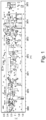
- Fig. 1 Based on the conventional approach with established state-of-the-art and Fig. 1 The result of the determination of the defect geometry shown above results in the mentioned maximum burst pressure of 4744.69 kPa.
Landscapes
- Chemical & Material Sciences (AREA)
- Life Sciences & Earth Sciences (AREA)
- Health & Medical Sciences (AREA)
- Physics & Mathematics (AREA)
- General Physics & Mathematics (AREA)
- Immunology (AREA)
- Pathology (AREA)
- General Health & Medical Sciences (AREA)
- Biochemistry (AREA)
- Analytical Chemistry (AREA)
- Chemical Kinetics & Catalysis (AREA)
- Engineering & Computer Science (AREA)
- Electrochemistry (AREA)
- Theoretical Computer Science (AREA)
- Software Systems (AREA)
- Crystallography & Structural Chemistry (AREA)
- Medicinal Chemistry (AREA)
- Food Science & Technology (AREA)
- Medical Informatics (AREA)
- Evolutionary Computation (AREA)
- General Engineering & Computer Science (AREA)
- Computing Systems (AREA)
- Data Mining & Analysis (AREA)
- Mathematical Physics (AREA)
- Artificial Intelligence (AREA)
- Computer Vision & Pattern Recognition (AREA)
- Management, Administration, Business Operations System, And Electronic Commerce (AREA)
- Investigating Or Analyzing Materials By The Use Of Magnetic Means (AREA)
- Testing Of Devices, Machine Parts, Or Other Structures Thereof (AREA)
- Monitoring And Testing Of Nuclear Reactors (AREA)
Claims (15)
- Procédé permettant de déterminer la géométrie d'une ou de plusieurs imperfections examinées, réelles, d'un objet magnétisable, en particulier d'un tuyau ou d'un réservoir, avec un jeu de données de référence généré sur la base d'une ou de plusieurs mesures MFL de l'objet,comprenant une représentation au moins partielle de l'objet au moyen d'une unité informatique, en particulier sur ou par une grille d'objet au moins tridimensionnelle, ainsi que comprenant une détermination d'une géométrie d'imperfection initiale en tant que géométrie d'imperfection de sortie, en particulier sur la grille d'objet ou une grille de défaut (15) au moins bidimensionnelle,une détermination d'un premier jeu de données de prédiction MFL en tant que jeu de données de prédiction de sortie sur la base de la géométrie d'imperfection de sortie, en particulier par une simulation d'une mesure MFL ou l'attribution d'un jeu de données MFL,et une adaptation itérative de la géométrie d'imperfection de sortie à la géométrie de la ou des imperfections réelles au moyen de l'unité informatique et au moyen de plusieurs routines expertes (11) s'exécutant en concurrence et de préférence en parallèle les unes aux autres de telle sorte que les routines expertes se font concurrence pour les ressources de l'unité informatique, dans lequel une géométrie d'imperfection experte est générée dans des routines expertes (11) respectives au moyen d'au moins un algorithme propre et sur la base de la géométrie d'imperfection de sortie,un jeu de données de prédiction expert respectif est déterminé sur la base de la géométrie d'imperfection experte respective, en particulier par la simulation d'une mesure MFL ou l'attribution d'un jeu de données MFL,et la géométrie d'imperfection experte à la base du jeu de données de prédiction expert respectif est mise à la disposition au moins de plusieurs, en particulier de toutes les routines expertes (11) en tant que nouvelle géométrie d'imperfection de sortie pour une adaptation supplémentaire à la géométrie de la ou des imperfections réelles,lorsque le jeu de données de prédiction expert ressemble plus au jeu de données de référence que le jeu de données de prédiction de sortie, et ensuite le jeu de données de prédiction expert appartenant à la nouvelle géométrie d'imperfection de sortie est utilisé en tant que nouveau jeu de données de prédiction de sortie,dans lequel l'adaptation itérative est effectuée au moyen des routines expertes jusqu'à ce qu'un critère d'arrêt soit satisfait.
- Procédé selon la revendication 1, caractérisé en que les routines expertes (11) s'exécutent en concurrence les unes avec les autres de telle sorte qu'une distribution des ressources de l'unité informatique à une routine experte respective, en particulier sous la forme d'un temps de calcul, de préférence d'un temps de CPU et/ou de GPU, est effectuée en fonction d'un taux de réussite, dans laquelle en particulier le nombre de géométries d'imperfection de sortie calculées par cette routine experte et mises à la disposition d'une ou de plusieurs autres routines expertes (11) est pris en compte, et/ou est effectuée en fonction d'une réduction d'une fonction de pertinence dans laquelle en particulier le nombre des jeux de données de prédiction experts générés pour la réduction est pris en compte.
- Procédé selon l'une quelconque des revendications précédentes, caractérisé en ce qu'une fonction de pertinence est utilisée en tant que mesure de la similitude des jeux de données de prédiction experts et de référence.
- Procédé selon l'une quelconque des revendications précédentes, caractérisé en ce que pour la détermination de la géométrie de la ou des imperfections, en plus un jeu de données de référence supplémentaire, indépendant linéairement du premier jeu de données de référence en ce qui concerne la magnétisation, est utilisé, et sur la base de la géométrie d'imperfection de sortie, un jeu de données de prédiction de sortie supplémentaire est déterminé en particulier au moyen d'une simulation MFL supplémentaire tenant compte de l'indépendance linéaire, et une géométrie d'imperfection experte n'est utilisée en tant que géométrie d'imperfection de sortie que si les jeux de données de prédiction experts associés, déterminés pour les deux magnétisations indépendantes, ressemblent plus aux jeux de données de référence respectifs que les jeux de données de prédiction de sortie déterminés pour les deux magnétisations et/ou une fonction de pertinence tenant compte des deux jeux de données de prédiction experts est améliorée.
- Procédé selon la revendication 4, caractérisé en ce que le premier jeu de données de référence a été généré par l'intermédiaire d'une mesure MFL avec une magnétisation axiale, et le deuxième jeu de données de référence a été généré par l'intermédiaire d'une mesure MFL avec une magnétisation dans la direction circonférentielle du tuyau.
- Procédé selon l'une quelconque des revendications précédentes, caractérisé en ce que les jeux de données de prédiction de sortie et/ou experts sont générés sur la base d'un modèle direct pour la simulation de la mesure MFL et en particulier au moyen d'un modèle à éléments finis.
- Procédé selon l'une quelconque des revendications précédentes, caractérisé en ce que la géométrie d'imperfection initiale est générée au moyen d'une table de recherche par l'une des routines expertes (11) et/ou par un algorithme d'apprentissage machine.
- Procédé selon l'une quelconque des revendications précédentes, caractérisé en ce que la grille de défaut (5) est affinée dans des zones où la profondeur de la ou des imperfections simulées dépasse une valeur seuil.
- Procédé selon l'une quelconque des revendications précédentes, caractérisé en ce que la grille d'objet et/ou de défaut (15) est affinée avant le calcul d'un jeu de données de prédiction expert respectif.
- Procédé selon l'une quelconque des différences précédentes, caractérisé en ce que la géométrie d'imperfection de sortie ou un pointeur s'y référant est sauvegardé(e) dans une zone de mémoire (12) accessible à toutes les routines expertes (11) de l'unité informatique.
- Procédé selon l'une quelconque des revendications précédentes, caractérisé en ce qu'une absence de modification de la géométrie d'imperfection de sortie et/ou de la géométrie de la grille d'objet et/ou de défaut (15) et/ou du jeu de données de prédiction de sortie et/ou d'au moins un jeu de données de prédiction expert après une pluralité d'itérations est adoptée en tant que critère d'arrêt.
- Procédé selon la revendication 11, caractérisé en ce qu'une comparaison de la variation du jeu de données de prédiction expert avec la dispersion de mesure du jeu de données réel est utilisée en tant que critère d'arrêt.
- Procédé selon l'une quelconque des revendications précédentes, caractérisé en ce que plusieurs algorithmes d'adaptation de la géométrie d'imperfection experte, comprenant un apprentissage machine, une optimisation stochastique, des fonctions modèles empiriques et/ou numériques, sont attribués à une routine experte (11).
- Procédé selon la revendication 13, caractérisé en ce que dans une routine experte (11), un algorithme est généré de manière aléatoire ou est sélectionné et/ou modifié par une fonction de sélection.
- Procédé permettant de déterminer une limite de capacité de charge d'un objet sous pression au moins en cours de fonctionnement, et réalisé en particulier sous forme d'oléoduc, de gazoduc ou d'aqueduc, dans lequel un jeu de données décrivant une ou plusieurs imperfections est utilisé comme jeu de données d'entrée dans un calcul de la limite de capacité de charge, caractérisé en ce que le jeu de données d'entrée est d'abord déterminé selon un procédé selon l'une quelconque des revendications précédentes.
Priority Applications (14)
| Application Number | Priority Date | Filing Date | Title |
|---|---|---|---|
| ES17195267T ES3040734T3 (en) | 2017-10-06 | 2017-10-06 | Method for determining the geometry of a defect and for determining a load capacity limit |
| EP17195267.4A EP3467489B1 (fr) | 2017-10-06 | 2017-10-06 | Procédé de détermination de la géométrie d'un défaut et de détermination de la capacité de charge |
| CN201880078530.4A CN111448453B (zh) | 2017-10-06 | 2018-09-28 | 确定缺陷的几何结构的方法以及确定负荷能力极限的方法 |
| CN202411159762.6A CN119165042A (zh) | 2017-10-06 | 2018-09-28 | 确定缺陷的几何结构的方法以及确定负荷能力极限的方法 |
| PCT/EP2018/076514 WO2019068588A1 (fr) | 2017-10-06 | 2018-09-28 | Procédé de détermination de la géométrie d'un défaut et de détermination de la limite de charge |
| CA3109990A CA3109990A1 (fr) | 2017-10-06 | 2018-09-28 | Procede de determination de la geometrie d'un defaut et de determination de la limite de charge |
| MX2020003580A MX2020003580A (es) | 2017-10-06 | 2018-09-28 | Procedimiento para determinar la geometria de un defecto y para determinar un limite de carga. |
| AU2018344386A AU2018344386B2 (en) | 2017-10-06 | 2018-09-28 | Method for determining the geometry of a defect and for determining a load limit |
| EP18782929.6A EP3692362A1 (fr) | 2017-10-06 | 2018-09-28 | Procédé de détermination de la géométrie d'un défaut et de détermination de la limite de charge |
| UAA202002574A UA126485C2 (uk) | 2017-10-06 | 2018-09-28 | Способи визначення геометрії дефекту матеріалу і визначення межі навантажувальної здатності |
| US16/753,919 US11624728B2 (en) | 2017-10-06 | 2018-09-28 | Method for determining the geometry of a defect and for determining a load limit |
| RU2020114878A RU2763344C2 (ru) | 2017-10-06 | 2018-09-28 | Способы определения геометрии дефекта материала и определения предела нагрузочной способности |
| US18/184,304 US20230258599A1 (en) | 2017-10-06 | 2023-03-15 | Method for determining the geometry of a defect and for determining a load limit |
| AU2024220204A AU2024220204B2 (en) | 2017-10-06 | 2024-09-30 | Method for determining the geometry of a defect and for determining a load limit |
Applications Claiming Priority (1)
| Application Number | Priority Date | Filing Date | Title |
|---|---|---|---|
| EP17195267.4A EP3467489B1 (fr) | 2017-10-06 | 2017-10-06 | Procédé de détermination de la géométrie d'un défaut et de détermination de la capacité de charge |
Publications (3)
| Publication Number | Publication Date |
|---|---|
| EP3467489A1 EP3467489A1 (fr) | 2019-04-10 |
| EP3467489C0 EP3467489C0 (fr) | 2025-06-25 |
| EP3467489B1 true EP3467489B1 (fr) | 2025-06-25 |
Family
ID=60117492
Family Applications (2)
| Application Number | Title | Priority Date | Filing Date |
|---|---|---|---|
| EP17195267.4A Active EP3467489B1 (fr) | 2017-10-06 | 2017-10-06 | Procédé de détermination de la géométrie d'un défaut et de détermination de la capacité de charge |
| EP18782929.6A Pending EP3692362A1 (fr) | 2017-10-06 | 2018-09-28 | Procédé de détermination de la géométrie d'un défaut et de détermination de la limite de charge |
Family Applications After (1)
| Application Number | Title | Priority Date | Filing Date |
|---|---|---|---|
| EP18782929.6A Pending EP3692362A1 (fr) | 2017-10-06 | 2018-09-28 | Procédé de détermination de la géométrie d'un défaut et de détermination de la limite de charge |
Country Status (10)
| Country | Link |
|---|---|
| US (2) | US11624728B2 (fr) |
| EP (2) | EP3467489B1 (fr) |
| CN (2) | CN119165042A (fr) |
| AU (2) | AU2018344386B2 (fr) |
| CA (1) | CA3109990A1 (fr) |
| ES (1) | ES3040734T3 (fr) |
| MX (1) | MX2020003580A (fr) |
| RU (1) | RU2763344C2 (fr) |
| UA (1) | UA126485C2 (fr) |
| WO (1) | WO2019068588A1 (fr) |
Families Citing this family (5)
| Publication number | Priority date | Publication date | Assignee | Title |
|---|---|---|---|---|
| ES2998810T3 (en) * | 2019-04-09 | 2025-02-21 | Rosen Ip Ag | Method for determining the geometry of an object based on data from nondestructive measurement methods |
| ES2903199T3 (es) * | 2019-04-09 | 2022-03-31 | Rosen Swiss Ag | Método para la determinación de la geometría de un punto defectuoso y para la determinación de un límite de la capacidad de carga |
| CN111444628B (zh) * | 2020-04-13 | 2022-06-24 | 中国石油大学(北京) | 射流清管器结构阻力计算方法及装置 |
| CN117009869A (zh) * | 2023-07-31 | 2023-11-07 | 广东利元亨智能装备股份有限公司 | 一种电芯外观检测方法、装置、计算机设备及存储介质 |
| CN119846052A (zh) * | 2025-03-18 | 2025-04-18 | 成都理工大学 | 一种适用于多尺寸连续油管损伤检测的试验测试系统 |
Citations (1)
| Publication number | Priority date | Publication date | Assignee | Title |
|---|---|---|---|---|
| US20160245779A1 (en) * | 2014-07-11 | 2016-08-25 | Halliburton Energy Services, Inc. | Evaluation tool for concentric wellbore casings |
Family Cites Families (34)
| Publication number | Priority date | Publication date | Assignee | Title |
|---|---|---|---|---|
| EP0164057A3 (fr) * | 1984-06-08 | 1988-05-04 | Mecapec S.A. | Procédés et appareils pour détecter des défauts de surface sur un objet ferromagnétique en forme de barre |
| US5223114A (en) * | 1987-06-17 | 1993-06-29 | Board Of Trustees Of The Leland Stanford Junior University | On-column conductivity detector for microcolumn electrokinetic separations |
| JPH08228632A (ja) * | 1995-02-27 | 1996-09-10 | Kyoei Seisakusho:Kk | 鑑賞魚用水槽の水質表示方式と水質表示装置 |
| US6208983B1 (en) * | 1998-01-30 | 2001-03-27 | Sarnoff Corporation | Method and apparatus for training and operating a neural network for detecting breast cancer |
| US6316937B1 (en) * | 1999-10-13 | 2001-11-13 | Oilfield Equipment Marketing, Inc. | Method and apparatus for detecting and measuring axially extending defects in ferrous tube |
| US6519535B1 (en) * | 2000-06-05 | 2003-02-11 | The University Of Chicago | Eddy current technique for predicting burst pressure |
| US7013224B2 (en) * | 2002-07-15 | 2006-03-14 | General Electric Company | Method and apparatus to perform crack estimations for nuclear reactor |
| US8050874B2 (en) * | 2004-06-14 | 2011-11-01 | Papadimitriou Wanda G | Autonomous remaining useful life estimation |
| US7414395B2 (en) * | 2006-03-27 | 2008-08-19 | General Electric Company | Method and apparatus inspecting pipelines using magnetic flux sensors |
| CN100483126C (zh) * | 2006-12-08 | 2009-04-29 | 清华大学 | 基于三维有限元神经网络的缺陷识别和量化评价方法 |
| US7987150B1 (en) * | 2007-02-09 | 2011-07-26 | Siglaz | Method and apparatus for automated rule-based sourcing of substrate microfabrication defects |
| JP5186837B2 (ja) * | 2007-08-23 | 2013-04-24 | Jfeスチール株式会社 | 微小凹凸表面欠陥の検出方法及び装置 |
| JP4938695B2 (ja) * | 2008-01-23 | 2012-05-23 | 富士通株式会社 | き裂進展評価装置及びき裂進展評価方法 |
| US8494827B2 (en) * | 2009-09-25 | 2013-07-23 | Exxonmobil Upstream Research Company | Method of predicting natural fractures and damage in a subsurface region |
| DE102010020149A1 (de) * | 2010-05-11 | 2011-11-17 | Frank Hoffmann | System zur automatischen Überprüfung von schadhaften Bauteilen an Maschinen und Anlagen |
| US9305121B2 (en) * | 2010-06-28 | 2016-04-05 | Exxonmobil Upstream Research Company | Method and system for modeling fractures in ductile rock |
| CN102368283A (zh) * | 2011-02-21 | 2012-03-07 | 麦克奥迪实业集团有限公司 | 一种基于数字切片的数字病理远程诊断系统及其方法 |
| DE102011000917B4 (de) * | 2011-02-24 | 2017-08-17 | Vallourec Deutschland Gmbh | Streuflusssonde zur zerstörungsfreien Streuflussprüfung von Körpern aus magnetisierbarem Werkstoff |
| US11029283B2 (en) * | 2013-10-03 | 2021-06-08 | Schlumberger Technology Corporation | Pipe damage assessment system and method |
| US9892219B2 (en) * | 2014-01-28 | 2018-02-13 | Rolls-Royce Corporation | Using fracture mechanism maps to predict time-dependent crack growth behavior under dwell conditions |
| CN104034794B (zh) * | 2014-06-12 | 2017-01-04 | 东北大学 | 一种基于极限学习机的管道漏磁缺陷检测方法 |
| US10613244B2 (en) * | 2014-07-11 | 2020-04-07 | Halliburton Energy Services, Inc. | Focused symmetric pipe inspection tools |
| RU2586261C2 (ru) * | 2014-08-13 | 2016-06-10 | Открытое акционерное общество "Акционерная компания по транспорту нефти "Транснефть" (ОАО "АК "Транснефть") | Устройство магнитного дефектоскопа и способ уменьшения погрешности определения размеров дефектов трубопровода магнитными дефектоскопами |
| CN104514987B (zh) * | 2014-12-19 | 2017-02-22 | 清华大学 | 管道三维漏磁成像缺陷量化方法 |
| CN104897771B (zh) * | 2015-05-12 | 2018-01-23 | 清华大学 | 三维漏磁检测缺陷轮廓重构方法及装置 |
| CN104899440B (zh) * | 2015-06-02 | 2017-09-29 | 上海电力学院 | 一种基于万有引力搜索算法的漏磁缺陷重构方法 |
| CN104990977B (zh) * | 2015-06-29 | 2018-02-09 | 清华大学 | 三维漏磁检测缺陷神经网络迭代反演成像方法 |
| US9715034B2 (en) * | 2015-12-18 | 2017-07-25 | Schlumberger Technology Corporation | Method for multi-tubular evaluation using induction measurements |
| CN105807743A (zh) * | 2016-03-15 | 2016-07-27 | 国网江苏省电力公司电力科学研究院 | 变电站设备故障缺陷分析远程支撑系统 |
| EP3475769B1 (fr) * | 2016-06-22 | 2020-05-13 | Saudi Arabian Oil Company | Systèmes et procédés pour la prédiction rapide de la fissuration induite par l'hydrogène (hic) dans des pipelines, des récipients sous pression et des systèmes de tuyauterie et pour entreprendre une action en rapport avec celle-ci |
| CN106018545B (zh) * | 2016-06-29 | 2019-05-14 | 东北大学 | 一种基于Adaboost-RBF协同的管道缺陷漏磁反演方法 |
| CN106709522B (zh) * | 2016-12-29 | 2020-03-10 | 武汉大学 | 一种基于改进模糊三角数的高压电缆施工缺陷分级方法 |
| CN106950276B (zh) * | 2017-03-21 | 2020-05-05 | 东北大学 | 一种基于卷积神经网络的管道缺陷深度的反演方法 |
| CN106975736A (zh) * | 2017-05-16 | 2017-07-25 | 南通江中光电有限公司 | 一种复杂薄壁铝合金梯级压铸成型技术 |
-
2017
- 2017-10-06 ES ES17195267T patent/ES3040734T3/es active Active
- 2017-10-06 EP EP17195267.4A patent/EP3467489B1/fr active Active
-
2018
- 2018-09-28 US US16/753,919 patent/US11624728B2/en active Active
- 2018-09-28 CA CA3109990A patent/CA3109990A1/fr active Pending
- 2018-09-28 EP EP18782929.6A patent/EP3692362A1/fr active Pending
- 2018-09-28 MX MX2020003580A patent/MX2020003580A/es unknown
- 2018-09-28 WO PCT/EP2018/076514 patent/WO2019068588A1/fr not_active Ceased
- 2018-09-28 UA UAA202002574A patent/UA126485C2/uk unknown
- 2018-09-28 AU AU2018344386A patent/AU2018344386B2/en active Active
- 2018-09-28 RU RU2020114878A patent/RU2763344C2/ru active
- 2018-09-28 CN CN202411159762.6A patent/CN119165042A/zh active Pending
- 2018-09-28 CN CN201880078530.4A patent/CN111448453B/zh active Active
-
2023
- 2023-03-15 US US18/184,304 patent/US20230258599A1/en active Pending
-
2024
- 2024-09-30 AU AU2024220204A patent/AU2024220204B2/en active Active
Patent Citations (1)
| Publication number | Priority date | Publication date | Assignee | Title |
|---|---|---|---|---|
| US20160245779A1 (en) * | 2014-07-11 | 2016-08-25 | Halliburton Energy Services, Inc. | Evaluation tool for concentric wellbore casings |
Also Published As
| Publication number | Publication date |
|---|---|
| AU2024220204A1 (en) | 2024-10-17 |
| EP3467489C0 (fr) | 2025-06-25 |
| AU2018344386A1 (en) | 2020-05-07 |
| ES3040734T3 (en) | 2025-11-04 |
| US20200340948A1 (en) | 2020-10-29 |
| MX2020003580A (es) | 2020-09-21 |
| EP3467489A1 (fr) | 2019-04-10 |
| CN111448453B (zh) | 2024-09-13 |
| AU2024220204B2 (en) | 2026-02-19 |
| RU2020114878A3 (fr) | 2021-11-08 |
| US20230258599A1 (en) | 2023-08-17 |
| CN111448453A (zh) | 2020-07-24 |
| AU2018344386B2 (en) | 2024-07-04 |
| EP3692362A1 (fr) | 2020-08-12 |
| UA126485C2 (uk) | 2022-10-12 |
| WO2019068588A1 (fr) | 2019-04-11 |
| CA3109990A1 (fr) | 2019-04-11 |
| RU2020114878A (ru) | 2021-11-08 |
| CN119165042A (zh) | 2024-12-20 |
| RU2763344C2 (ru) | 2021-12-28 |
| US11624728B2 (en) | 2023-04-11 |
Similar Documents
| Publication | Publication Date | Title |
|---|---|---|
| EP3467489B1 (fr) | Procédé de détermination de la géométrie d'un défaut et de détermination de la capacité de charge | |
| EP3722800B1 (fr) | Procédé de détermination de la géométrie d'un point défectueux sur la base d'un procédé de mesure non destructive à l'aide d'une inversion directe | |
| EP2999998B1 (fr) | Méthode de détermination d'un modèle d'une grandeur de sortie d'un système technique | |
| DE102018108778B4 (de) | Beschleunigungs- und verzögerungssteuereinheit, maschinenlernvorrichtung und maschinenlernverfahren | |
| EP3268713B1 (fr) | Procédé de réalisation d'un ensemble de modèles permettant d'étalonner un appareil de commande | |
| DE112012001851T5 (de) | Ermitteln von Fluid-Leckagevolumen in Pipelines | |
| DE102019209540A1 (de) | Verfahren und Vorrichtung zur optimalen Aufteilung von Testfällen auf unterschiedliche Testplattformen | |
| EP3722798B1 (fr) | Procédé de détermination de la géométrie d'un point défectueux et de détermination de la capacité de charge | |
| EP3267338A1 (fr) | Procede de calcul de contraintes en fond d'entaille dans un cordon de soudure | |
| EP1830235A2 (fr) | Conception d'outils et de processus pour technique de formage | |
| EP4222470B1 (fr) | Procede et dispositif informatiques pour la prediction de vitesse basee sur la probabilite pour des vehicules | |
| DE102016201559A1 (de) | Verfahren und Vorrichtung zum Vermessen eines zu testenden Systems | |
| EP3708945B1 (fr) | Évaluation des données de mesure d'une mesure d'une pluralité de pièces | |
| EP3740904B1 (fr) | Procédé de fonctionnement d'un réseau neuronal artificiel | |
| DE102020205962B3 (de) | Vorrichtung und Verfahren zum Betreiben eines Prüfstands | |
| DE10146901A1 (de) | Verfahren und System zur Bearbeitung von Fehlerhypothesen | |
| DE102023134513A1 (de) | Statistische visualisierungen und anomaliedetektion für fahrzeugkalibrierungssätze | |
| EP3722799A1 (fr) | Procédé de détermination de la géométrie d'un objet en fonction des données du procédé de mesure non destructive | |
| EP3980850B1 (fr) | Génération de données actives en tenant compte des incertitudes | |
| EP2996001A1 (fr) | Procédé d'analyse assisté par ordinateur d'un ensemble de données provenant d'observations | |
| DE102019002506A1 (de) | Gerät zum Anpassen von Messvorgangsparametern, maschinelle Lernvorrichtung und System | |
| EP4075223A1 (fr) | Analyse des causes en cas d'anomalies du fonctionnement d'une installation technique | |
| DE102024204014A1 (de) | Systematische auswahl repräsentativer muster für serienprodukte | |
| DE102019129385A1 (de) | Verfahren zur automatisierten Ermittlung von Kennlinien und/oder Kennfeldern | |
| DE102023203628A1 (de) | Verfahren zur Vorverarbeitung von Codedaten für eine anschließende Auswertung |
Legal Events
| Date | Code | Title | Description |
|---|---|---|---|
| PUAI | Public reference made under article 153(3) epc to a published international application that has entered the european phase |
Free format text: ORIGINAL CODE: 0009012 |
|
| STAA | Information on the status of an ep patent application or granted ep patent |
Free format text: STATUS: THE APPLICATION HAS BEEN PUBLISHED |
|
| AK | Designated contracting states |
Kind code of ref document: A1 Designated state(s): AL AT BE BG CH CY CZ DE DK EE ES FI FR GB GR HR HU IE IS IT LI LT LU LV MC MK MT NL NO PL PT RO RS SE SI SK SM TR |
|
| AX | Request for extension of the european patent |
Extension state: BA ME |
|
| STAA | Information on the status of an ep patent application or granted ep patent |
Free format text: STATUS: REQUEST FOR EXAMINATION WAS MADE |
|
| 17P | Request for examination filed |
Effective date: 20190906 |
|
| RBV | Designated contracting states (corrected) |
Designated state(s): AL AT BE BG CH CY CZ DE DK EE ES FI FR GB GR HR HU IE IS IT LI LT LU LV MC MK MT NL NO PL PT RO RS SE SI SK SM TR |
|
| STAA | Information on the status of an ep patent application or granted ep patent |
Free format text: STATUS: EXAMINATION IS IN PROGRESS |
|
| 17Q | First examination report despatched |
Effective date: 20200508 |
|
| RAP1 | Party data changed (applicant data changed or rights of an application transferred) |
Owner name: ROSEN IP AG |
|
| GRAP | Despatch of communication of intention to grant a patent |
Free format text: ORIGINAL CODE: EPIDOSNIGR1 |
|
| STAA | Information on the status of an ep patent application or granted ep patent |
Free format text: STATUS: GRANT OF PATENT IS INTENDED |
|
| GRAS | Grant fee paid |
Free format text: ORIGINAL CODE: EPIDOSNIGR3 |
|
| INTG | Intention to grant announced |
Effective date: 20240913 |
|
| GRAJ | Information related to disapproval of communication of intention to grant by the applicant or resumption of examination proceedings by the epo deleted |
Free format text: ORIGINAL CODE: EPIDOSDIGR1 |
|
| GRAL | Information related to payment of fee for publishing/printing deleted |
Free format text: ORIGINAL CODE: EPIDOSDIGR3 |
|
| STAA | Information on the status of an ep patent application or granted ep patent |
Free format text: STATUS: EXAMINATION IS IN PROGRESS |
|
| GRAP | Despatch of communication of intention to grant a patent |
Free format text: ORIGINAL CODE: EPIDOSNIGR1 |
|
| STAA | Information on the status of an ep patent application or granted ep patent |
Free format text: STATUS: GRANT OF PATENT IS INTENDED |
|
| INTC | Intention to grant announced (deleted) | ||
| INTG | Intention to grant announced |
Effective date: 20250203 |
|
| GRAA | (expected) grant |
Free format text: ORIGINAL CODE: 0009210 |
|
| STAA | Information on the status of an ep patent application or granted ep patent |
Free format text: STATUS: THE PATENT HAS BEEN GRANTED |
|
| AK | Designated contracting states |
Kind code of ref document: B1 Designated state(s): AL AT BE BG CH CY CZ DE DK EE ES FI FR GB GR HR HU IE IS IT LI LT LU LV MC MK MT NL NO PL PT RO RS SE SI SK SM TR |
|
| REG | Reference to a national code |
Ref country code: GB Ref legal event code: FG4D Free format text: NOT ENGLISH |
|
| REG | Reference to a national code |
Ref country code: CH Ref legal event code: EP |
|
| REG | Reference to a national code |
Ref country code: CH Ref legal event code: EP |
|
| REG | Reference to a national code |
Ref country code: IE Ref legal event code: FG4D Free format text: LANGUAGE OF EP DOCUMENT: GERMAN |
|
| REG | Reference to a national code |
Ref country code: DE Ref legal event code: R096 Ref document number: 502017016917 Country of ref document: DE |
|
| U01 | Request for unitary effect filed |
Effective date: 20250722 |
|
| U07 | Unitary effect registered |
Designated state(s): AT BE BG DE DK EE FI FR IT LT LU LV MT NL PT RO SE SI Effective date: 20250729 |
|
| PG25 | Lapsed in a contracting state [announced via postgrant information from national office to epo] |
Ref country code: GR Free format text: LAPSE BECAUSE OF FAILURE TO SUBMIT A TRANSLATION OF THE DESCRIPTION OR TO PAY THE FEE WITHIN THE PRESCRIBED TIME-LIMIT Effective date: 20250926 |
|
| PG25 | Lapsed in a contracting state [announced via postgrant information from national office to epo] |
Ref country code: HR Free format text: LAPSE BECAUSE OF FAILURE TO SUBMIT A TRANSLATION OF THE DESCRIPTION OR TO PAY THE FEE WITHIN THE PRESCRIBED TIME-LIMIT Effective date: 20250625 |
|
| PG25 | Lapsed in a contracting state [announced via postgrant information from national office to epo] |
Ref country code: RS Free format text: LAPSE BECAUSE OF FAILURE TO SUBMIT A TRANSLATION OF THE DESCRIPTION OR TO PAY THE FEE WITHIN THE PRESCRIBED TIME-LIMIT Effective date: 20250925 |
|
| REG | Reference to a national code |
Ref country code: CH Ref legal event code: U11 Free format text: ST27 STATUS EVENT CODE: U-0-0-U10-U11 (AS PROVIDED BY THE NATIONAL OFFICE) Effective date: 20251101 |
|
| REG | Reference to a national code |
Ref country code: ES Ref legal event code: FG2A Ref document number: 3040734 Country of ref document: ES Kind code of ref document: T3 Effective date: 20251104 |
|
| U20 | Renewal fee for the european patent with unitary effect paid |
Year of fee payment: 9 Effective date: 20251027 |
|
| PG25 | Lapsed in a contracting state [announced via postgrant information from national office to epo] |
Ref country code: IS Free format text: LAPSE BECAUSE OF FAILURE TO SUBMIT A TRANSLATION OF THE DESCRIPTION OR TO PAY THE FEE WITHIN THE PRESCRIBED TIME-LIMIT Effective date: 20251025 |
|
| PGFP | Annual fee paid to national office [announced via postgrant information from national office to epo] |
Ref country code: GB Payment date: 20251024 Year of fee payment: 9 |
|
| PGFP | Annual fee paid to national office [announced via postgrant information from national office to epo] |
Ref country code: NO Payment date: 20251022 Year of fee payment: 9 |
|
| PG25 | Lapsed in a contracting state [announced via postgrant information from national office to epo] |
Ref country code: SM Free format text: LAPSE BECAUSE OF FAILURE TO SUBMIT A TRANSLATION OF THE DESCRIPTION OR TO PAY THE FEE WITHIN THE PRESCRIBED TIME-LIMIT Effective date: 20250625 |
|
| PGFP | Annual fee paid to national office [announced via postgrant information from national office to epo] |
Ref country code: CH Payment date: 20251101 Year of fee payment: 9 |
|
| PG25 | Lapsed in a contracting state [announced via postgrant information from national office to epo] |
Ref country code: CZ Free format text: LAPSE BECAUSE OF FAILURE TO SUBMIT A TRANSLATION OF THE DESCRIPTION OR TO PAY THE FEE WITHIN THE PRESCRIBED TIME-LIMIT Effective date: 20250625 |
|
| PG25 | Lapsed in a contracting state [announced via postgrant information from national office to epo] |
Ref country code: PL Free format text: LAPSE BECAUSE OF FAILURE TO SUBMIT A TRANSLATION OF THE DESCRIPTION OR TO PAY THE FEE WITHIN THE PRESCRIBED TIME-LIMIT Effective date: 20250625 |
|
| PG25 | Lapsed in a contracting state [announced via postgrant information from national office to epo] |
Ref country code: SK Free format text: LAPSE BECAUSE OF FAILURE TO SUBMIT A TRANSLATION OF THE DESCRIPTION OR TO PAY THE FEE WITHIN THE PRESCRIBED TIME-LIMIT Effective date: 20250625 |
|
| PGFP | Annual fee paid to national office [announced via postgrant information from national office to epo] |
Ref country code: ES Payment date: 20251114 Year of fee payment: 9 |