EP3637139A1 - Simulation de faisceaux de détection et de télémétrie de lumière - Google Patents
Simulation de faisceaux de détection et de télémétrie de lumière Download PDFInfo
- Publication number
- EP3637139A1 EP3637139A1 EP18199900.4A EP18199900A EP3637139A1 EP 3637139 A1 EP3637139 A1 EP 3637139A1 EP 18199900 A EP18199900 A EP 18199900A EP 3637139 A1 EP3637139 A1 EP 3637139A1
- Authority
- EP
- European Patent Office
- Prior art keywords
- ray
- intersection
- reflected
- energy
- rays
- Prior art date
- Legal status (The legal status is an assumption and is not a legal conclusion. Google has not performed a legal analysis and makes no representation as to the accuracy of the status listed.)
- Withdrawn
Links
Images

Classifications
-
- G—PHYSICS
- G01—MEASURING; TESTING
- G01S—RADIO DIRECTION-FINDING; RADIO NAVIGATION; DETERMINING DISTANCE OR VELOCITY BY USE OF RADIO WAVES; LOCATING OR PRESENCE-DETECTING BY USE OF THE REFLECTION OR RERADIATION OF RADIO WAVES; ANALOGOUS ARRANGEMENTS USING OTHER WAVES
- G01S17/00—Systems using the reflection or reradiation of electromagnetic waves other than radio waves, e.g. lidar systems
- G01S17/006—Theoretical aspects
-
- G—PHYSICS
- G06—COMPUTING OR CALCULATING; COUNTING
- G06F—ELECTRIC DIGITAL DATA PROCESSING
- G06F30/00—Computer-aided design [CAD]
- G06F30/20—Design optimisation, verification or simulation
Definitions
- the present invention is related to a method of simulating a LIght Detection And Ranging (LIDAR) beam.
- the present invention is related to simulating a LIDAR beam through ray-tracing.
- LIDAR LIght Detection And Ranging
- LIDAR is an optical method for measuring distance and velocity as well as for measuring atmospheric parameters. Laser rays or beams of several rays are used for the measuring.
- LIDAR is used as a measuring instrument for stationary and mobile speed monitoring. In the field of construction and surveying, LIDAR is used for distance measuring. Further, in Automatic Driver Assistance Systems (ADAS), and in autonomous vehicles, LIDAR is used for both measuring distance, e.g. to detect objects in the surroundings of a vehicle and to create a virtual map of said surroundings, and measuring velocity, e.g. to implement a collision warning. Moreover, in the field of aviation, LIDAR is also used for detecting turbulences and wind shear. Consequently, the measurements done with LIDAR must be reliable and precise because critical decisions are based thereon.
- ADAS Automatic Driver Assistance Systems
- LIDAR is also used for detecting turbulences and wind shear. Consequently, the measurements done with LIDAR must be reliable and precise because critical decisions are based thereon.
- a method of simulating a LIght Detection And Ranging (LIDAR) beam of a LIDAR sensor in a scene comprises the following sequential steps:
- a LIDAR beam is characterised by several parameters: e.g. the beam cross-section, the beam divergence, the beam emission pattern and the beam pulse pattern.
- a LIDAR beam commonly used in automotive has a rectangular or square cross-section within which a laser or multiple lasers have a emission pattern comprising horizontal or vertical rows/stripes or any other suitable pattern including meander shapes, circles, ellipses, spirals, a Gaussian configuration and the like.
- the beam may originate from a point source or several point sources defining a source area. From the point source or the source area the beam diverges with a certain divergence angle or divergence angles, which may be measured relative to the emission direction of the point source or source area, respectively.
- the beam has a certain initial source area some distance away from the actual point source.
- the beam is always simulated starting from a source area.
- the source area is discretised into separate origins.
- the source area may be discretised into 100.000 or less, preferably 10.000 or less and most preferably 4000 or less origins.
- Each origin can be the origin of one single ray of the LIDAR beam.
- Each ray has a certain emitting direction such that the LIDAR beam is simulated as a truncated pyramid of arbitrary cross-sectional shape like a frustum originating at the source area and diverging with a certain angle of divergence from the emission direction of the source area.
- the direction of each ray may be characterised by two divergence angles, ⁇ and ⁇ .
- the two divergence angles may each be within one of two perpendicular planes spanned by the emission direction and a respective radial direction perpendicular to the emission direction.
- rays are selected based on the origins.
- Each of the origins may emit one single ray of the LIDAR beam that is simulated as a truncated pyramid of arbitrary cross-sectional shape (e.g. frustum). Thereby, each ray has a certain direction along which the ray radiates from the source area.
- the number of rays, that is selected based on the respective origins may be deliberately predetermined. Consequently only a subset of the whole LIDAR beam is selected. However, increasing the number of rays also increases the precision of the simulation results.
- the rays may be selected according to a certain pattern or rule or randomly.
- the rays originating from the source area are simulated with a time varying energy distribution.
- the energy distribution is modelled as the time based energy distribution of a laser pulse. This energy distribution is contained in a vector of time bins, where every time bin contains a certain energy value of the ray.
- the time bins may have a size of about 1 ps [Picosecond] to about 1 ns [Nanosecond], preferably of about 1 ps, more preferably of about 10 ps and most preferably of about 100 ps.
- Each of the selected rays is simulated propagating through the scene or environment and interacting with the objects in the scene.
- ray-tracing is a method to sample geometry in a virtual scene known from computer graphics.
- ray-tracing is used to create an image by shooting rays from a camera and instantaneously (no propagation time) accumulate light on a sensor pixel.
- the selected rays (of the laser) are shot originating from the respective origin of the source area and connected to the LIDAR sensor, where light energy is accumulated in the (time varying) signal.
- ray-tracing in the present invention does not ignore propagation time of the rays.
- step c2) for each of the rays the reflected energy of the current ray is determined.
- the current ray interacts with the surface of the object.
- One part of the energy of the current ray is reflected back towards the LIDAR sensor as the reflected energy.
- the amount of energy that is reflected back depends on a material and surface of the object.
- the interactions with the objects in the scene may be calculated based on radiance rather than energy with the Bidirectional Scattering Distribution Function (BSDF). If the BSDF is used, the radiance is only converted into the unit of energy when the reflected energy is added to the signal.
- BSDF Bidirectional Scattering Distribution Function
- the reflected energy represents a time varying energy distribution.
- the energy distribution of the reflected energy corresponds to the energy (or radiance) of the laser pulse that is reflected from the surface object at the intersection.
- the reflected energy (distribution) is sent back to the (virtual) LIDAR sensor where it is sensed over time. Additionally, there may be a check whether the path along which the reflected energy travels from the intersection to the (virtual) LIDAR sensor is not blocked or occluded by an object or other occlusion.
- the visibility of the intersection from the view point of the (virtual) LIDAR sensor is determined with a shadow ray cast from the (virtual) LIDAR sensor to the respective intersection.
- the energy distribution of the reflected energy is contained in a vector of time bins.
- the time bins may have a size of about 1 ps to about 1 ns, preferably of about 1 ps, more preferably of about 10 ps and most preferably of about 100 ps.
- the reflected energy is added to the signal, representing the signal of the real LIDAR sensor.
- step c3 If no intersection of a current ray occurs during ray-tracing in step c1) then according to step c3) for each of the rays, the next ray is ray-traced in step c1). Consequently, each of the selected rays is ray-traced and, if an intersection is found, the reflected energy based on the current ray is added to the signal of the LIDAR sensor.
- the resulting signal containing the summed up reflected energies is outputted to another method or system or a user.
- the signal can alternatively or additionally be stored in a storage device.
- the energy distribution of the LIDAR beam with all its rays is considered in the simulation such that a full physics based simulation is enabled, where the LIDAR beam is fully simulated.
- arbitrary material properties can be used in the simulation and a full-waveform signal is computed.
- This enables a more precise simulation of the actual signal of the real LIDAR sensor because all interactions of the beam and its scattered rays with the environment (objects in the scene) are simulated. Consequently, LIDAR systems can be configured with better tolerance and be tested and validated with higher precision. This adds to security for example in autonomous vehicles and ADAS systems for modern vehicles.
- step b) the rays are randomly selected.
- the rays are randomly selected based on at least one random number and preferably based on two random numbers.
- the selection of rays used for the simulation of the LIDAR beam can be effected with the help of one single random number.
- the origins of the discretised surface area can be consecutively numbered and the rays can be selected by randomly choosing numbers of the origins.
- the selection of rays can be based on two random numbers. For example two random numbers each for one of the two deflection angles can be randomly chosen or the origins can be numbered according to their position in a x direction (dim x) and a perpendicular y direction (dim y) and the origins of the rays can be randomly chosen based on these two dimensions.
- Selecting the rays based on one or two random numbers is a very efficient way of determining the set of rays used for simulation of the LIDAR beam.
- the rays are randomly selected by importance sampling, low discrepancy sampling patterns or deterministic sampling patterns.
- Importance sampling is a general technique for estimating properties of the LIDAR beam, while only having samples generated from a different distribution namely the selected rays than the distribution of interest namely the whole beam.
- Low-discrepancy sampling patterns are quasi-random or sub-random patterns, due to their use as a replacement of uniformly distributed random numbers for choosing the rays.
- quasi-Monte-Carlo method the lower discrepancy of the low-discrepancy sampling patterns is an important advantage.
- the deterministic character of deterministic sampling patterns the latter can be used instead of a random selection scheme and nevertheless produce a suitably distributed selection of rays just like the random schemes mentioned before.
- step b) at least two, preferably at least 100, more preferably at least 500 and most preferably at least 1000 rays are selected.
- step b) at most 100000, preferably at most 10000, more preferably at most 5000 and most preferably at most 2000 rays are selected.
- the signal is distributed over time represented by a vector of time bins.
- the vector has a length corresponding to a predetermined sampling time T S .
- the rays have an energy that is represented as a time varying energy distribution which is contained in a vector of time bins.
- the signal is represented by a vector with a length corresponding to the sampling time Ts.
- the sampling time Ts can be about 100 ns to 50000 ns and preferably about 500 ns to 2000 ns.
- the time bins may have a size of about 1 ps [Picosecond] to about 1 ns [Nanosecond], preferably of about 1 ps, more preferably of about 10 ps and most preferably of about 100 ps.
- the energy distributions of the reflected energies are sampled at the time point when they hit the LIDAR sensor and added bin-wise to the signal.
- step c2) further comprises the following steps if an intersection is found:
- step c1 If an intersection of the current ray (originally emitted ray or scattered ray, respectively) is detected in step c1) the total length of the current ray from the respective origin to the intersection or the total length of the scattered ray from the respective origin to the last intersection (along all preceding intersections) s I is used together with the speed of light c to calculate the travel time of the respective ray.
- the respective intersection time point t I is then calculated based on the time point of radiation t R , which is the time point, when the respective ray was emitted from the source area.
- t I t R + s I c
- the sensing time point ts when the reflected energy is sensed at the LIDAR sensor is calculated based on the intersection time point t I and the length between the intersection and the LIDAR sensor s S , wherein the length of path along which the reflected energy travels from the intersection to the LIDAR sensor is also determined by ray-tracing.
- t S t I + s S c
- the reflected energy is added to the signal at said sensing time point t S .
- step of determining a scattered ray comprises reducing the current ray by the reflected energy.
- the current ray or the scattered ray, respectively is reduced by the determined reflected energy that is reflected back to the LIDAR sensor from the surface of the object.
- the interactions between the current ray (originally emitted ray or scattered ray, respectively) and the objects in the scene may be calculated using the BSDF, using the unit of radiance rather than the unit of energy.
- the current ray may be "continued" in the scattered direction reduced by the reflected energy.
- step c2) further comprises the following steps if an intersection is found:
- step c2) for each of the rays the scattered ray is additionally determined.
- the current ray interacts with the surface of the object.
- One part of the energy of the current ray is reflected back towards the LIDAR sensor as the reflected energy.
- the remaining energy of the current ray is scattered into a different direction with a certain scattering angle that depends on the material and surface of the object.
- the scattered ray is continued to be simulated. So, instead of continuing with the next ray of the LIDAR beam, the scattered ray is ray-traced through the scene, by continuing with step c1) for the scattered ray.
- the reflected energy is determined, this time based on the scattered ray, and added to the signal. There may be a check whether the reflected energy can propagate from the intersection to the (virtual) LIDAR sensor without any occlusion. Thereto, via a shadow ray the visibility of the respective intersection from the view point of the (virtual) LIDAR sensor is checked, wherein the shadow ray is cast from the (virtual) LIDAR sensor to the respective intersection.
- the scattered ray (which is the current ray in this iteration) is also scattered such that a (twofold) scattered ray is continued to be simulated.
- step c1) is executed for the newly (twofold) scattered ray.
- the ray-tracing for scattered rays continues as long as an intersection at the surface of an object in the scene occurs for the scattered rays.
- a lower threshold for the energy of the scattered ray down to which it is simulated and/or a maximal number of reflections/bounces e.g. 10 reflections
- step c3 If no (more) intersection of a current ray (originally emitted ray or scattered ray, respectively) occurs during ray-tracing in step c1) then according to step c3) for each of the rays, the next ray is ray-traced in step c1). Consequently, each of the selected rays is ray-traced and, if an intersection is found, scattered and, in turn, the resulting scattered ray is traced until no more intersection with an object in the scene occurs or optionally until the lower threshold for the energy of the ray or the maximal number of reflections is reached. At each intersection the reflected energy based on the current ray (originally emitted or scattered ray, respectively) is added to the signal of the LIDAR sensor.
- the resulting signal containing the summed up reflected energies is outputted to another method or system or a user.
- the signal can alternatively or additionally be stored in a storage device.
- step of determining a scattered ray comprises reducing the current ray by the reflected energy.
- the current ray or the scattered ray, respectively is reduced by the determined reflected energy that is reflected back to the LIDAR sensor from the surface of the object.
- the interactions between the current ray (originally emitted ray or scattered ray, respectively) and the objects in the scene may be calculated using the BSDF, using the unit of radiance rather than the unit of energy.
- the current ray may be "continued" in the scattered direction reduced by the reflected energy.
- the reflected energies of precedent beams are accounted for in the present beam.
- the processing unit may be controlled by a program implementing the method as described above.
- a flow chart of a method 10 of simulating a LIght Detection And Ranging (LIDAR) beam of a LIDAR sensor in a scene is schematically depicted.
- the method comprises a first step a) of discretising 11 a source area, a subsequent second step b) of selecting 12 rays, a subsequent third iteration step c) for ray-tracing 13 and a fourth step of storing and/or outputting 14.
- the third iteration step c) for ray-tracing 13 comprises a first step c1) of finding 15 an intersection, a subsequent second iteration step c2) for signal calculation 16 and a third step c3) of continuing 17 with step c1).
- the second iteration step c2) for signal calculation comprises a step of determining 16.1 a reflected energy, a step of calculating 16.2 an intersection time point t I , a step of calculating 16.3 a sensing time point ts, a step of adding 16.4 the reflected energy, a step of determining 16.5 a scattered ray and a step of continuing 16.6 with step c1).
- the source area of the LIDAR beam is discretised into origins in the first step a) of discretising 11.
- Each origin is the basis from which one single ray of the LIADR beam is emitted in a specific direction.
- the direction is given by two divergence angles ⁇ and ⁇ measured against the emission direction on the source area.
- each ray represents a time varying energy distribution of a laser pulse.
- the energy distribution of the laser pulse is simulated as a normal distribution contained in a vector of time bins.
- the time bins have a size of 100 ps [Picoseconds].
- the vector of the ray has a total length of 10 ns [Nanoseconds] containing 100 bins.
- each of the (originally emitted) rays or scattered rays is traced and an intersection with an object in a virtual scene is searched according to the first step c1) of finding 15. If an intersection is found the second iteration step c2) for signal calculation 16 is executed.
- a reflected energy is determined based on the material and surface of the object in the step of determining 16.1 for the current ray or the scattered ray (see below).
- the reflected energy represents a time varying energy distribution of the reflected energy corresponding to the energy of the laser pulse that is reflected from the surface object at the intersection.
- the reflected energy (distribution) is sent back to the (virtual) LIDAR sensor where it is sensed over time.
- the energy distribution of the reflected energy is contained in a vector of time bins.
- the time bins have a size of 100 ps and the vector of the reflected energy has a total length of 10 ns containing 100 bins.
- the reflected energy is added to the signal representing the signal of the real LIDAR sensor.
- an intersection time point t I is calculated in the step of calculating 16.2 based on a radiation time point t R of the respective ray, which is the time point, when the respective ray was emitted from the source area, and a total length of the current ray from the respective origin to the intersection or the total length of a scattered ray (see below) from the respective origin to the last intersection (along all preceding intersections) s I together with the speed of light c.
- t I t R + s I c
- a sensing time point ts giving the time point when the reflected energy is sensed at the LIDAR sensor, is calculated based on the intersection time point t I and the length between the intersection and the LIDAR sensor s S , wherein the length of path along which the reflected energy travels from the intersection to the LIDAR sensor is also determined by ray-tracing.
- t S t I + s S c
- the vector of the reflected energy (100 bins of 100 ps each) is added in the step of adding 16.4 to the signal at said sensing time point t S .
- the signal is distributed over time represented by a vector of time bins of 100 ps.
- the vector has a total length corresponding to a sampling time T S of 700 ns and containing 7000 bins.
- a scattered ray is determined based on the surface and material of the object at the intersection.
- the scattered ray has an energy distribution according to the ray but reduced by the scattered energy.
- the scattered ray leaves the intersection under a scattering angle depending on the surface and material of the object at the intersection.
- step c1) of finding 15 If an intersection was found in step c1) of finding 15 the method 10 is continued in the step of continuing 16.6 at step c1) of finding 15 with the scattered ray as current ray.
- step c1) of finding 15 If no intersection is found in step c1) of finding 15, then the method is continued in the step c3) of continuing 17 at step c1) of finding 15 with the next ray as current ray until all rays are processed.
- the method is continued at the step d) of storing or outputting 14, where the added up signal is output to another method and/or system and/or to a user and/or stored in a storage.
- the method 10 may also consider reflected energies from (originally emitted) rays or scattered rays of preceding beams in the step of adding 16.5, when the reflected energy arrives at the (virtual) LIDAR sensor after the sampling time T s .
- reflected energies that are not considered in the signal of the beam that effected the reflected energies because they arrive "belated" after the sampling time Ts can be considered in the signal of the next beam.
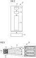
- a system 20 for simulating a LIDAR beam of a LIDAR sensor in a scene comprises a processing unit 21 and a storage and/or output 22.
- the processing unit has a discretising module 23 configured for discretising a source area of the LIDAR beam into separate origins, a selecting module 24 configured for selecting rays based on the origins, wherein each ray represents a time varying energy distribution of a laser pulse contained in a vector of time bins, and a ray-tracing module 25.
- the ray-tracing module 25 is configured for finding an intersection of the current ray with an object of the scene through ray-tracing for each ray.
- the ray-tracing module is further configured for determining a reflected energy of the current ray that is reflected from the object at the intersection back to the LIDAR sensor if an intersection is found, wherein the reflected energy represents a time varying energy distribution corresponding to the energy of the laser pulse reflected from the object at the intersection back over time contained in a vector of time bins.
- the ray-tracing module 25 is configured for calculating an intersection time point t I based on a radiation time point t R of the current ray and on a length of the current ray from its origin to the intersection s I and for calculating a sensing time point ts of sensing the reflected energy at the LIDAR sensor based on the intersection time point t I and on the length of a distance from the intersection to the LIDAR sensor s S , wherein in the step of adding the reflected energy, the reflected energy is added to the signal at the sensing time point t S . Additionally, the ray-tracing module 25 is configured for adding the reflected energy to a signal if an intersection is found.
- the ray-tracing module 25 is configured for determining a scattered ray based on the current ray scattered from the object at the intersection if an intersection is found and for reducing the current ray by the reflected energy as well as for continuing with finding an intersection of the current ray for the scattered ray. Lastly, the ray-tracing module is also configured for continuing with finding an intersection of the current ray for the next ray.
- the storage 22 is configured for storing the added up signal and the output 22 configured for outputting the added up signal.
- the processing unit 21 can be a Central Processing Unit (CPU) or Graphics Processing Unit (GPU) like a Microcontroller (pC), an integrated circuit, an Application-Specific Integrated Circuit (ASIC), an Application-Specific Standard Product (ASSP), a Digital Signal Processor (DSP), a Field Programmable Gate Array (FPGA) and the like.
- the processing unit 21 may be controlled by a program implementing the method of Fig. 1 or as described above.
- the modules 23 to 25 may be part of the processing unit 21 or implemented on the processing unit 21 or separate units in communicative connection with the processing unit 21.
- the storage 22 can be a data storage like a magnetic storage/memory (e.g.
- magnetic-core memory magnetic tape, magnetic card, magnet strip, magnet bubble storage, drum storage, hard disc drive, floppy disc or removable storage
- an optical storage/memory e.g. holographic memory, optical tape, Tesa tape, Laserdisc, Phasewriter (Phasewriter Dual, PD), Compact Disc (CD), Digital Video Disc (DVD), High Definition DVD (HD DVD), Bluray Disc (BD) or Ultra Density Optical (UDO)
- a magneto-optical storage/memory e.g. MiniDisc or Magneto-Optical Disk (MO-Disk)
- a volatile semiconductor/solid state memory e.g.
- RAM Random Access Memory
- DRAM Dynamic RAM
- SRAM Static RAM
- a non-volatile semiconductor/solid state memory e.g. Read Only Memory (ROM), Programmable ROM (PROM), Erasable PROM (EPROM), Electrically EPROM (EEPROM), Flash-EEPROM (e.g. USB-Stick), Ferroelectric RAM (FRAM), Magnetoresistive RAM (MRAM) or Phase-change RAM
- the output 22 may be any kind of port or link or interface capable of communicating information to another (e.g. WLAN, Bluetooth, ZigBee, Profibus, ETHERNET etc.) system or to a user (Display, Printer, Speaker etc.).
- a LIDAR beam 30 is schematically depicted.
- the LIDAR beam 30 has a rectangular source area 31 with a first dimension dim X and a second dimension dim Y.
- the LIDAR beam is made up by three striped emission pattern of a single laser diode scanning the environment or scene.
- the LIDAR beam 30 is made up by rays 33 originating from the source area 31 and each projecting from one origin of the source area 31 in a unique direction defined by ⁇ and ⁇ .
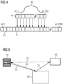
- each ray of the LIDAR beam may be represented by an energy distribution.
- This energy distribution corresponds to an energy distribution of a laser pulse of a LIDAR sensor.
- the energy distribution of the laser pulse is simulated as a normal distribution.
- the energy distribution 40 of the reflected energy is also a normal distribution.
- multi-bounce ray-tracing is schematically depicted.
- a ray 32 originating from the source area 31 is scattered at an object 50 one part of its energy is reflected back to the LIDAR sensor as reflected energy 52.
- the ray is also continued as scattered ray 51 reduced by the reflected energy 52.
- the scattered ray is scattered at another object 50 and part of the energy of the scattered ray 51 is reflected back to the LIDAR sensor as another reflected energy 53.
- This multi-bounce ray-tracing may be executed for any arbitrary number of scatterings of one ray 33.
Landscapes
- Engineering & Computer Science (AREA)
- Physics & Mathematics (AREA)
- General Physics & Mathematics (AREA)
- Theoretical Computer Science (AREA)
- Evolutionary Computation (AREA)
- General Engineering & Computer Science (AREA)
- Geometry (AREA)
- Computer Hardware Design (AREA)
- Computer Networks & Wireless Communication (AREA)
- Electromagnetism (AREA)
- Radar, Positioning & Navigation (AREA)
- Remote Sensing (AREA)
- Optical Radar Systems And Details Thereof (AREA)
Priority Applications (2)
| Application Number | Priority Date | Filing Date | Title |
|---|---|---|---|
| EP18199900.4A EP3637139A1 (fr) | 2018-10-11 | 2018-10-11 | Simulation de faisceaux de détection et de télémétrie de lumière |
| PCT/EP2019/076532 WO2020074311A1 (fr) | 2018-10-11 | 2019-10-01 | Simulation de faisceaux de détection et télémétrie par ondes lumineuses |
Applications Claiming Priority (1)
| Application Number | Priority Date | Filing Date | Title |
|---|---|---|---|
| EP18199900.4A EP3637139A1 (fr) | 2018-10-11 | 2018-10-11 | Simulation de faisceaux de détection et de télémétrie de lumière |
Publications (1)
| Publication Number | Publication Date |
|---|---|
| EP3637139A1 true EP3637139A1 (fr) | 2020-04-15 |
Family
ID=63833933
Family Applications (1)
| Application Number | Title | Priority Date | Filing Date |
|---|---|---|---|
| EP18199900.4A Withdrawn EP3637139A1 (fr) | 2018-10-11 | 2018-10-11 | Simulation de faisceaux de détection et de télémétrie de lumière |
Country Status (2)
| Country | Link |
|---|---|
| EP (1) | EP3637139A1 (fr) |
| WO (1) | WO2020074311A1 (fr) |
Families Citing this family (1)
| Publication number | Priority date | Publication date | Assignee | Title |
|---|---|---|---|---|
| CN119644300A (zh) * | 2023-09-18 | 2025-03-18 | 上海禾赛科技有限公司 | 用于对激光雷达的工作过程进行仿真的方法和计算设备 |
-
2018
- 2018-10-11 EP EP18199900.4A patent/EP3637139A1/fr not_active Withdrawn
-
2019
- 2019-10-01 WO PCT/EP2019/076532 patent/WO2020074311A1/fr not_active Ceased
Non-Patent Citations (2)
| Title |
|---|
| ANGELA M. KIM: "SIMULATING FULL-WAVEFORM LIDAR", THESES AND DISSERTATIONS, 1 September 2010 (2010-09-01), XP055574612, Retrieved from the Internet <URL:https://calhoun.nps.edu/bitstream/handle/10945/4538/09Sep_Kim.pdf?sequence=1&isAllowed=y> [retrieved on 20190326] * |
| PETER SHIRLEY ET AL: "Monte Carlo techniques for direct lighting calculations", ACM TRANSACTIONS ON GRAPHICS (TOG), ACM, US, vol. 15, no. 1, 1 January 1996 (1996-01-01), pages 1 - 36, XP058303297, ISSN: 0730-0301, DOI: 10.1145/226150.226151 * |
Also Published As
| Publication number | Publication date |
|---|---|
| WO2020074311A1 (fr) | 2020-04-16 |
Similar Documents
| Publication | Publication Date | Title |
|---|---|---|
| US11460562B2 (en) | Methods to simulate continuous wave lidar sensors | |
| US7652620B2 (en) | RCS signature generation for closely spaced multiple objects using N-point models | |
| US10133834B2 (en) | Method for simulating wave propagation; simulator, computer program and recording medium for implementing the method | |
| CN107003398B (zh) | 针对机动车安全雷达系统的使用虚拟雷达特征信号的测试方法 | |
| Hanke et al. | Generation and validation of virtual point cloud data for automated driving systems | |
| US11846727B2 (en) | System and method for emulating echo signals for a LiDAR sensor | |
| CN112505643A (zh) | 一种雷达与红外复合导引头开环半实物仿真方法及系统 | |
| Ngo et al. | A multi-layered approach for measuring the simulation-to-reality gap of radar perception for autonomous driving | |
| CN112652045A (zh) | 一种面向自动驾驶虚实融合测试的点云融合方法及其应用 | |
| Hasirlioglu et al. | A model-based approach to simulate rain effects on automotive surround sensor data | |
| EP3637138A1 (fr) | Simulation de faisceaux de détection et de télémétrie de lumière | |
| Rosenberger et al. | Benchmarking and functional decomposition of automotive lidar sensor models | |
| Rosenberger et al. | Analysis of real world sensor behavior for rising fidelity of physically based lidar sensor models | |
| CN115731350A (zh) | 车辆的虚拟激光雷达的仿真方法及其装置 | |
| EP3637139A1 (fr) | Simulation de faisceaux de détection et de télémétrie de lumière | |
| Chen et al. | Analysis of real-time lidar sensor simulation for testing automated driving functions on a vehicle-in-the-loop testbench | |
| CN116628953A (zh) | 一种虚拟点云的模拟方法及装置 | |
| US12164031B2 (en) | Method and system for a threshold noise filter | |
| US11995761B2 (en) | Methods and system for generating virtual sensor data of a virtual single-photon avalanche diode (SPAD) lidar sensor of a virtual vehicle simulator | |
| Hofrichter et al. | Fmcw lidar simulation with ray tracing and standardized interfaces | |
| CN115542294A (zh) | 一种基于时域路径追踪的激光雷达脉冲回波仿真方法 | |
| US20240427021A1 (en) | Real-time simulation of a laser beam scanning of a complex of small objects | |
| Schabus et al. | Object-Based Lidar Model for Enhanced Sensor Simulation in Automated Driving | |
| JPH02300692A (ja) | 降水量計量方法 | |
| Prabakaran et al. | Simulation of weather conditions perturbation for an automotive LIDAR sensor |
Legal Events
| Date | Code | Title | Description |
|---|---|---|---|
| PUAI | Public reference made under article 153(3) epc to a published international application that has entered the european phase |
Free format text: ORIGINAL CODE: 0009012 |
|
| STAA | Information on the status of an ep patent application or granted ep patent |
Free format text: STATUS: THE APPLICATION HAS BEEN PUBLISHED |
|
| AK | Designated contracting states |
Kind code of ref document: A1 Designated state(s): AL AT BE BG CH CY CZ DE DK EE ES FI FR GB GR HR HU IE IS IT LI LT LU LV MC MK MT NL NO PL PT RO RS SE SI SK SM TR |
|
| AX | Request for extension of the european patent |
Extension state: BA ME |
|
| STAA | Information on the status of an ep patent application or granted ep patent |
Free format text: STATUS: THE APPLICATION IS DEEMED TO BE WITHDRAWN |
|
| 18D | Application deemed to be withdrawn |
Effective date: 20201016 |