EP3658018B1 - Systèmes et procédés d'imagerie en écho de gradient acquise de façon stratégique - Google Patents
Systèmes et procédés d'imagerie en écho de gradient acquise de façon stratégique Download PDFInfo
- Publication number
- EP3658018B1 EP3658018B1 EP17918854.5A EP17918854A EP3658018B1 EP 3658018 B1 EP3658018 B1 EP 3658018B1 EP 17918854 A EP17918854 A EP 17918854A EP 3658018 B1 EP3658018 B1 EP 3658018B1
- Authority
- EP
- European Patent Office
- Prior art keywords
- map
- processor
- transmit
- field
- anatomical region
- Prior art date
- Legal status (The legal status is an assumption and is not a legal conclusion. Google has not performed a legal analysis and makes no representation as to the accuracy of the status listed.)
- Active
Links
Images






Classifications
-
- A—HUMAN NECESSITIES
- A61—MEDICAL OR VETERINARY SCIENCE; HYGIENE
- A61B—DIAGNOSIS; SURGERY; IDENTIFICATION
- A61B5/00—Measuring for diagnostic purposes; Identification of persons
- A61B5/0033—Features or image-related aspects of imaging apparatus, e.g. for MRI, optical tomography or impedance tomography apparatus; Arrangements of imaging apparatus in a room
- A61B5/004—Features or image-related aspects of imaging apparatus, e.g. for MRI, optical tomography or impedance tomography apparatus; Arrangements of imaging apparatus in a room adapted for image acquisition of a particular organ or body part
- A61B5/0042—Features or image-related aspects of imaging apparatus, e.g. for MRI, optical tomography or impedance tomography apparatus; Arrangements of imaging apparatus in a room adapted for image acquisition of a particular organ or body part for the brain
-
- A—HUMAN NECESSITIES
- A61—MEDICAL OR VETERINARY SCIENCE; HYGIENE
- A61B—DIAGNOSIS; SURGERY; IDENTIFICATION
- A61B5/00—Measuring for diagnostic purposes; Identification of persons
- A61B5/05—Detecting, measuring or recording for diagnosis by means of electric currents or magnetic fields; Measuring using microwaves or radio waves
- A61B5/055—Detecting, measuring or recording for diagnosis by means of electric currents or magnetic fields; Measuring using microwaves or radio waves involving electronic [EMR] or nuclear [NMR] magnetic resonance, e.g. magnetic resonance imaging
-
- G—PHYSICS
- G01—MEASURING; TESTING
- G01R—MEASURING ELECTRIC VARIABLES; MEASURING MAGNETIC VARIABLES
- G01R33/00—Arrangements or instruments for measuring magnetic variables
- G01R33/20—Arrangements or instruments for measuring magnetic variables involving magnetic resonance
- G01R33/44—Arrangements or instruments for measuring magnetic variables involving magnetic resonance using nuclear magnetic resonance [NMR]
- G01R33/48—NMR imaging systems
- G01R33/4818—MR characterised by data acquisition along a specific k-space trajectory or by the temporal order of k-space coverage, e.g. centric or segmented coverage of k-space
-
- G—PHYSICS
- G01—MEASURING; TESTING
- G01R—MEASURING ELECTRIC VARIABLES; MEASURING MAGNETIC VARIABLES
- G01R33/00—Arrangements or instruments for measuring magnetic variables
- G01R33/20—Arrangements or instruments for measuring magnetic variables involving magnetic resonance
- G01R33/44—Arrangements or instruments for measuring magnetic variables involving magnetic resonance using nuclear magnetic resonance [NMR]
- G01R33/48—NMR imaging systems
- G01R33/50—NMR imaging systems based on the determination of relaxation times, e.g. T1 measurement by IR sequences; T2 measurement by multiple-echo sequences
-
- G—PHYSICS
- G01—MEASURING; TESTING
- G01R—MEASURING ELECTRIC VARIABLES; MEASURING MAGNETIC VARIABLES
- G01R33/00—Arrangements or instruments for measuring magnetic variables
- G01R33/20—Arrangements or instruments for measuring magnetic variables involving magnetic resonance
- G01R33/44—Arrangements or instruments for measuring magnetic variables involving magnetic resonance using nuclear magnetic resonance [NMR]
- G01R33/48—NMR imaging systems
- G01R33/54—Signal processing systems, e.g. using pulse sequences ; Generation or control of pulse sequences; Operator console
- G01R33/56—Image enhancement or correction, e.g. subtraction or averaging techniques, e.g. improvement of signal-to-noise ratio and resolution
- G01R33/5608—Data processing and visualization specially adapted for MR, e.g. for feature analysis and pattern recognition on the basis of measured MR data, segmentation of measured MR data, edge contour detection on the basis of measured MR data, for enhancing measured MR data in terms of signal-to-noise ratio by means of noise filtering or apodization, for enhancing measured MR data in terms of resolution by means for deblurring, windowing, zero filling, or generation of gray-scaled images, colour-coded images or images displaying vectors instead of pixels
-
- G—PHYSICS
- G01—MEASURING; TESTING
- G01R—MEASURING ELECTRIC VARIABLES; MEASURING MAGNETIC VARIABLES
- G01R33/00—Arrangements or instruments for measuring magnetic variables
- G01R33/20—Arrangements or instruments for measuring magnetic variables involving magnetic resonance
- G01R33/44—Arrangements or instruments for measuring magnetic variables involving magnetic resonance using nuclear magnetic resonance [NMR]
- G01R33/48—NMR imaging systems
- G01R33/54—Signal processing systems, e.g. using pulse sequences ; Generation or control of pulse sequences; Operator console
- G01R33/56—Image enhancement or correction, e.g. subtraction or averaging techniques, e.g. improvement of signal-to-noise ratio and resolution
- G01R33/561—Image enhancement or correction, e.g. subtraction or averaging techniques, e.g. improvement of signal-to-noise ratio and resolution by reduction of the scanning time, i.e. fast acquiring systems, e.g. using echo-planar pulse sequences
- G01R33/5613—Generating steady state signals, e.g. low flip angle sequences [FLASH]
-
- G—PHYSICS
- G01—MEASURING; TESTING
- G01R—MEASURING ELECTRIC VARIABLES; MEASURING MAGNETIC VARIABLES
- G01R33/00—Arrangements or instruments for measuring magnetic variables
- G01R33/20—Arrangements or instruments for measuring magnetic variables involving magnetic resonance
- G01R33/44—Arrangements or instruments for measuring magnetic variables involving magnetic resonance using nuclear magnetic resonance [NMR]
- G01R33/48—NMR imaging systems
- G01R33/54—Signal processing systems, e.g. using pulse sequences ; Generation or control of pulse sequences; Operator console
- G01R33/56—Image enhancement or correction, e.g. subtraction or averaging techniques, e.g. improvement of signal-to-noise ratio and resolution
- G01R33/561—Image enhancement or correction, e.g. subtraction or averaging techniques, e.g. improvement of signal-to-noise ratio and resolution by reduction of the scanning time, i.e. fast acquiring systems, e.g. using echo-planar pulse sequences
- G01R33/5615—Echo train techniques involving acquiring plural, differently encoded, echo signals after one RF excitation, e.g. using gradient refocusing in echo planar imaging [EPI], RF refocusing in rapid acquisition with relaxation enhancement [RARE] or using both RF and gradient refocusing in gradient and spin echo imaging [GRASE]
-
- G—PHYSICS
- G01—MEASURING; TESTING
- G01R—MEASURING ELECTRIC VARIABLES; MEASURING MAGNETIC VARIABLES
- G01R33/00—Arrangements or instruments for measuring magnetic variables
- G01R33/20—Arrangements or instruments for measuring magnetic variables involving magnetic resonance
- G01R33/44—Arrangements or instruments for measuring magnetic variables involving magnetic resonance using nuclear magnetic resonance [NMR]
- G01R33/48—NMR imaging systems
- G01R33/54—Signal processing systems, e.g. using pulse sequences ; Generation or control of pulse sequences; Operator console
- G01R33/56—Image enhancement or correction, e.g. subtraction or averaging techniques, e.g. improvement of signal-to-noise ratio and resolution
- G01R33/565—Correction of image distortions, e.g. due to magnetic field inhomogeneities
- G01R33/56554—Correction of image distortions, e.g. due to magnetic field inhomogeneities caused by acquiring plural, differently encoded echo signals after one RF excitation, e.g. correction for readout gradients of alternating polarity in EPI
-
- G—PHYSICS
- G01—MEASURING; TESTING
- G01R—MEASURING ELECTRIC VARIABLES; MEASURING MAGNETIC VARIABLES
- G01R33/00—Arrangements or instruments for measuring magnetic variables
- G01R33/20—Arrangements or instruments for measuring magnetic variables involving magnetic resonance
- G01R33/44—Arrangements or instruments for measuring magnetic variables involving magnetic resonance using nuclear magnetic resonance [NMR]
- G01R33/48—NMR imaging systems
- G01R33/54—Signal processing systems, e.g. using pulse sequences ; Generation or control of pulse sequences; Operator console
- G01R33/56—Image enhancement or correction, e.g. subtraction or averaging techniques, e.g. improvement of signal-to-noise ratio and resolution
- G01R33/567—Image enhancement or correction, e.g. subtraction or averaging techniques, e.g. improvement of signal-to-noise ratio and resolution gated by physiological signals, i.e. synchronization of acquired MR data with periodical motion of an object of interest, e.g. monitoring or triggering system for cardiac or respiratory gating
- G01R33/5676—Gating or triggering based on an MR signal, e.g. involving one or more navigator echoes for motion monitoring and correction
-
- A—HUMAN NECESSITIES
- A61—MEDICAL OR VETERINARY SCIENCE; HYGIENE
- A61B—DIAGNOSIS; SURGERY; IDENTIFICATION
- A61B2576/00—Medical imaging apparatus involving image processing or analysis
- A61B2576/02—Medical imaging apparatus involving image processing or analysis specially adapted for a particular organ or body part
- A61B2576/026—Medical imaging apparatus involving image processing or analysis specially adapted for a particular organ or body part for the brain
-
- A—HUMAN NECESSITIES
- A61—MEDICAL OR VETERINARY SCIENCE; HYGIENE
- A61B—DIAGNOSIS; SURGERY; IDENTIFICATION
- A61B5/00—Measuring for diagnostic purposes; Identification of persons
- A61B5/72—Signal processing specially adapted for physiological signals or for diagnostic purposes
- A61B5/7203—Signal processing specially adapted for physiological signals or for diagnostic purposes for noise prevention, reduction or removal
-
- A—HUMAN NECESSITIES
- A61—MEDICAL OR VETERINARY SCIENCE; HYGIENE
- A61B—DIAGNOSIS; SURGERY; IDENTIFICATION
- A61B5/00—Measuring for diagnostic purposes; Identification of persons
- A61B5/72—Signal processing specially adapted for physiological signals or for diagnostic purposes
- A61B5/7235—Details of waveform analysis
- A61B5/7264—Classification of physiological signals or data, e.g. using neural networks, statistical classifiers, expert systems or fuzzy systems
-
- G—PHYSICS
- G01—MEASURING; TESTING
- G01R—MEASURING ELECTRIC VARIABLES; MEASURING MAGNETIC VARIABLES
- G01R33/00—Arrangements or instruments for measuring magnetic variables
- G01R33/20—Arrangements or instruments for measuring magnetic variables involving magnetic resonance
- G01R33/24—Arrangements or instruments for measuring magnetic variables involving magnetic resonance for measuring direction or magnitude of magnetic fields or magnetic flux
- G01R33/246—Spatial mapping of the RF magnetic field B1
Definitions
- the present disclosure relates generally to the field of magnetic resonance imaging (MRI).
- this disclosure relates to methods and systems for quantitative magnetic resonance imaging (qMRI) using variable flip angle (VFA) techniques.
- Magnetic resonance imaging is an imaging modality that uses magnetic fields to reconstruct a structure of scanned objects of interest.
- An MRI scanner includes a magnet for generating a strong static magnetic field, such as a magnetic field in the range of 0.10 Tesla (T) to 7 T, and radio frequency (RF) transceivers for transmitting and/or receiving RF signals.
- a strong static magnetic field such as a magnetic field in the range of 0.10 Tesla (T) to 7 T
- RF radio frequency
- sampling time or echo time, or gradient echo time
- data is collected and the received signal is used to reconstruct an image of the scanned body or a part thereof.
- VFA techniques for reconstructing MR images based on collected MR datasets are described. N. Weiskopf et al "Unified segmentation based correction of R1 brain maps for RF transmit field inhomogeneities (UNICORT)" Neuroimage, vol.
- (2011 ) relates to simultaneous estimation of B1(+) inhomogeneities and R1 values from uncorrected R1 maps in the human brain without the need for B1(+) mapping by employing a probabilistic framework for unified segmentation based correction of R1 maps for B1(+) inhomogeneities.
- a magnetic resonance imaging (MRI) system can include a MRI scanner, at least one processor, and a memory, with computer code instructions stored thereon.
- the MRI scanner can be configured to acquire a first magnetic resonance (MR) dataset corresponding to a first flip angle and a second MR dataset corresponding to a second flip angle by imaging an anatomical region using at least one echo time.
- the computer code instructions when executed by the at least one processor, cause the at least one processor to generate an apparent longitudinal relaxation time (T 1app ) map, representing a spatial distribution of T1app within the anatomical region using the first MR dataset and the second MR dataset.
- the at least one processor can estimate a first transmit RF field map by scaling the T 1app map by a first constant value of longitudinal relaxation time (T 1 ).
- the first constant value of T 1 can be associated with a first tissue type within the anatomical region.
- the at least one processor can estimate a second transmit RF field map by scaling the T 1app map by a second constant value of T 1 .
- the second constant value of T 1 can be associated with a second tissue type within the anatomical region.
- the processor can generate a third transmit RF field map using the estimated first transmit RF field map and the estimated second transmit RF field map.
- the third transmit RF field map can represent a spatial distribution of the transmit RF field within the anatomical region.
- the anatomical region can be a human brain where the first tissue type can be white matter, and the second tissue type can be gray matter.
- the at least one processor can estimate a fourth transmit RF field map by scaling the T 1app map by a third constant value of T 1 .
- the third constant value of T 1 can be associated with a third tissue type within the anatomical region.
- Generating the third transmit RF field map can include using the estimated first transmit RF field map, the estimated second transmit RF field map, and the estimated fourth transmit RF field map.
- the anatomical region can be a human brain where the first tissue type can be white matter, the second tissue type can be gray matter, and the third tissue type can be cerebro-spinal fluid.
- the at least one processor can generate a first longitudinal relaxation time (T 1 ) map by dividing the T 1app map by the square of the third transmit RF field map.
- the first T 1 map can represent the spatial distribution of T 1 within the anatomical region.
- the at least one processor can generate an apparent spin density (SD app ) map using the first MR dataset and the second MR dataset.
- the SD app map can represent a spatial distribution of SD app within the anatomical region.
- the at least one processor can generate a first spin density (SD) map by scaling the SD app map by the third transmit RF field map.
- the at least one processor can synthesize, using the third transmit RF field map, the first T 1 map, and the first SD map, a third MR dataset corresponding to a third flip angle such that at least a first sub-region of the anatomical region corresponding to the first tissue type and a second sub-region of the anatomical region corresponding to the second tissue type are isointense.
- the at least one processor can estimate a receive RF field map using the synthesized third MR dataset.
- the receive RF field map can represent a spatial distribution of a receive RF field within the anatomical region.
- the at least one processor can generate a second SD map by scaling the first SD map by the estimated receive RF field map.
- the at least one processor can scale the first MR dataset by the receive RF field map, scale the second MR data set by the receive MR dataset, and generate an image representing a weighted subtraction of the scaled first MR dataset from the scaled second MR dataset.
- the at least one processor can generate an image representing a weighted subtraction of the first MR dataset from the second MR dataset.
- the at least one processor can estimate a plurality of transmit RF field maps for a plurality of subjects, and generate a transmit RF field template using an averaging of the estimated plurality of transmit RF field maps for the plurality of subjects.
- the at least one processor can generate a second T 1 map using the T 1app map and the transmit RF field template.
- the at least one processor can generate a spin density (SD) map using an estimated SD app map, the transmit RF field template, and an estimated receive RF field map.
- SD spin density
- a method for magnetic resonance imaging can include at least one processor receiving a first magnetic resonance (MR) dataset corresponding to a first flip angle and a second MR dataset corresponding to a second flip angle.
- the first MR dataset and the second MR dataset can be acquired by imaging an anatomical region using at least one echo time.
- the method can include the at least one processor generating an apparent longitudinal relaxation time (T 1app ) map, representing a spatial distribution of T 1app within the anatomical region using the first MR dataset and the second MR dataset within the anatomical region.
- the method can include the at least one processor estimating a first transmit RF field map by scaling the T 1app map by a first constant value of longitudinal relaxation time (T 1 ).
- the first constant value of T 1 can be associated with a first tissue type within the anatomical region.
- the method can include the at least one processor estimating a second transmit RF field map by scaling the T 1app map by a second constant value of T 1 .
- the second constant value of T 1 can be associated with a second tissue type within the anatomical region.
- the method can include the at least one processor generating a third transmit RF field map using the estimated first transmit RF field map and the estimated second transmit RF field map.
- the third transmit RF field map can represent a spatial distribution of the transmit RF field within the anatomical region.
- the method can further include the at least one processor estimating a fourth transmit RF field map by scaling the T 1app map by a third constant value of T 1 .
- the third constant value of T 1 can be associated with a third tissue type within the anatomical region.
- Generating the third transmit RF field map can include using the estimated first transmit RF field map, the estimated second transmit RF field map, and the estimated fourth transmit RF field map.
- the anatomical region can be a human brain where the first tissue type can be white matter, the second tissue type can be gray matter, and the third tissue type can be cerebro-spinal fluid.
- the method can further include the at least one processor generating a first longitudinal relaxation time (T 1 ) map by dividing the T 1app map by the square of the third transmit RF field map.
- the first T 1 map can represent the spatial distribution of T 1 within the anatomical region.
- the method can further include the at least one processor generating an apparent spin density (SD app ) map using the first MR dataset and the second MR dataset.
- the SD app map can represent a spatial distribution of SD app within the anatomical region.
- the at least one processor can generate a first spin density (SD) map by scaling the SD app map by the third transmit RF field map.
- the at least one processor can synthesize, using the third transmit RF field map, the first T 1 map, and the first SD map, a third MR dataset corresponding to a third flip angle such that at least a first sub-region of the anatomical region corresponding to the first tissue type and a second sub-region of the anatomical region corresponding to the second tissue type are isointense.
- the at least one processor can estimate a receive RF field map using the synthesized third MR dataset.
- the receive RF field map can represent a spatial distribution of a receive RF field within the anatomical region.
- the at least one processor can generate a second SD map by scaling the first SD map by the estimated receive RF field map.
- the method can further include the at least one processor scaling the first MR dataset by the receive RF field map, scaling the second MR data set by the receive MR dataset, and generating an image representing a weighted subtraction of the scaled first MR dataset from the scaled second MR dataset.
- the method can further include the at least one processor generating an image representing a weighted subtraction of the first MR dataset from the second MR dataset.
- the method can further include the at least one processor estimating a plurality of transmit RF field maps for a plurality of subjects, and generating a transmit RF field template using an averaging of the estimated plurality of transmit RF field maps for the plurality of subjects.
- the method can further include the at least one processor generating a second T 1 map using the T 1app map and the transmit RF field template.
- the method can further include the at least one processor generating a spin density (SD) map using an estimated SD app map, the transmit RF field template, and an estimated receive RF field map.
- SD spin density
- a computer-readable medium includes computer code instructions stored thereon.
- the computer code instructions when executed by at least one processor cause a method for magnetic resonance imaging (MRI) to be performed.
- the method can include the at least one processor receiving a first magnetic resonance (MR) dataset corresponding to a first flip angle and a second MR dataset corresponding to a second flip angle.
- the first MR dataset and the second MR dataset can be acquired by imaging an anatomical region using at least one echo time.
- the method can include the at least one processor generating an apparent longitudinal relaxation time (T 1app ) map, representing a spatial distribution of T 1app within the anatomical region using the first MR dataset, the second MR dataset and a constant value for a transmit radio frequency (RF) field within the anatomical region.
- T 1app apparent longitudinal relaxation time
- the method can include the at least one processor estimating a first transmit RF field map by scaling the T 1app map by a first constant value of longitudinal relaxation time (T 1 ).
- the first constant value of T 1 can be associated with a first tissue type within the anatomical region.
- the method can include the at least one processor estimating a second transmit RF field map by scaling the T 1app map by a second constant value of T 1 .
- the second constant value of T 1 can be associated with a second tissue type within the anatomical region.
- the method can include the at least one processor generating a third transmit RF field map using the estimated first transmit RF field map and the estimated second transmit RF field map.
- the third transmit RF field map can represent a spatial distribution of the transmit RF field within the anatomical region.
- Quantitative magnetic resonance imaging involves measuring and/or using signal intensities or relative signal intensities to distinguish between different types of tissues or to identify abnormal tissues. By quantifying the tissue properties, it becomes easier to develop methods to both segment and classify normal and abnormal tissue types.
- quantitative spin density SD
- T 1 longitudinal relaxation time
- T 2 * transverse magnetization decay rate
- QSM quantitative susceptibility mapping
- quantitative T 1 imaging has potential utility in studying atherosclerosis in cardiovascular imaging, tumors, stroke, and multiple sclerosis.
- quantitative SD mapping plays a significant role and has been used to study edema and changes in tissue water content after treatment. Generally, this type of tissue quantification makes it possible to follow the response of the tissue to treatment in a more rigorous fashion.
- VFA variable flip angle
- reconstruction of the SD map involves the use of the receive RF field (B 1r ) map.
- a MRI scanner or a respective processor can compute the transmit RF field B 1t by using acquired datasets for at least three different flip angles (FAs) including a dataset associated with a relatively large FA, for example, compared to the other two FAs.
- FAs flip angles
- Using datasets corresponding to less than three FAs or relatively small FAs can render the problem of constructing the transmit RF field B 1t ill-posed and can call for additional constraints to remedy the ill-posedness of the problem. Examples of such constraints to address the ill-posedness can include using a single tissue such as fat to determine the B 1t field distribution for breast imaging, or using constraints on the relationship between T 1 and SD for white matter and gray matter.
- STAGE imaging can allow for comprehensive rapid imaging using acquired datasets corresponding to two FAs. Also, the systems and methods for STAGE imaging described herein allow for reliable and accurate reconstruction of T1 and SD maps.
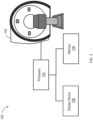
- FIG. 1 is a block diagram illustrating a magnetic resonance imaging (MRI) system 100, according to an aspect of the invention.
- the MRI system 100 includes a MRI scanner 102, a processor 104, a memory 106, and a display device 108.
- the processor 104 is communicatively coupled to the MRI scanner 102, the memory 106 and the display device 108.
- the MRI scanner 102 can include a magnet (not shown in FIG. 1 ) for generating a strong static magnetic field, such as a magnetic field in the range of 0.1 Tesla (T) to 7 T, and a plurality of radio frequency (RF) coils (not shown in FIG. 1 ) for transmitting and/or receiving RF signals.
- the RF coils can include transmit RF coils and receive RF coils.
- the RF transmit coils can emit RF pulses to excite a subject, such as an anatomical region of a patient, according to a MRI pulse sequence.
- the receive RF coils can record MRI signals generated by the subject following the emission of the RF pulses.
- the RF coils may include RF transceivers capable of alternately transmitting and receiving RF signals.
- the RF coils can acquire MRI data according to an RF spoiled gradient data acquisition.
- the recorded MRI signals can be associated with two different FAs.
- the imaging system 100 includes one or more processors 104.
- the one or more processors 104 can include a processor integrated within the MRI scanner 102, a processor of a computing device communicatively coupled to the MRI scanner 102, or a combination thereof.
- the memory 106 can include a memory component of the MRI scanner 102, a memory component of a computing device communicatively coupled to the MRI scanner 102, or a combination thereof.
- the memory 106 includes computer executable instructions, which when executed by the one or more processors 104, cause the one or more processors 104 to perform methods for STAGE imaging described herein.
- the memory 106 can store MRI data acquired by the MRI scanner 102, and the processor(s) 104 can access such data from the memory 106.
- the memory 106 can receive and store images generated by the processor(s) 104 based on the MRI data acquired by the scanner 102.
- the display device 108 can include a cathode ray tube (CRT) display, a light emitting diode (LED) display, an organic light emitting diode (OLED) display, a plasma display panel (PDP), a liquid crystal display (LCD), or other display known to a person of ordinary skill in the art.
- the display device 108 may be a stand-alone device or a display of a computing device (e.g., a desktop, laptop, or tablet) communicatively coupled to the MRI scanner 102.
- the display device 108 can include a touch screen.
- the display device 108 can receive image data from the processor 104 or the memory 106 and display the received image data.
- the processor 104 can provide the reconstructed images for display on the display device 108.
- T1 is the longitudinal relation time
- SD is the spin density
- TR is the repetition time
- TE the echo time
- B 1t is the transmit RF field
- B 1r is the receive RF field (also referred to as RF coil sensitivity or bias field)
- E1 exp(-TR/T 1 ).
- S ⁇ sin B 1 t ⁇ can be viewed as a linear function of S ⁇ tan B 1 t ⁇ .
- FIG. 2 is a flowchart illustrating a method 200 for magnetic resonance imaging (MRI).
- the method 200 includes obtaining (or receiving) a first magnetic resonance (MR) dataset corresponding to a first flip angle and a second MR dataset corresponding to a second flip angle (step 202), and generating an apparent longitudinal relaxation time (T 1app ) map using the first MR data, the second MR data and a constant value for a transmit radio frequency (RF) field within the anatomical region (step 204).
- MR magnetic resonance
- T 1app apparent longitudinal relaxation time
- the method 200 also includes estimating a first transmit RF field map by scaling the T 1app map by a first constant value of longitudinal relaxation time (T 1 ) (step 206), estimating a second transmit RF field map by scaling the T1app map by a second constant value of T 1 (step 208), and generating a third transmit RF field map using the estimated first transmit RF field map and the estimated second transmit RF field map (step 210).
- the method 200 includes obtaining (or receiving) a first magnetic resonance (MR) dataset corresponding to a first flip angle and a second MR dataset corresponding to a second flip angle (step 202).
- the scanner 102 can acquire the first MR dataset and the second MR dataset by imaging an anatomical region using at least one echo time TE.
- the processor 104 can provide a user interface (UI), e.g., on the display device 108, to allow a user to select settings for MR data acquisition.
- the processor 102 can cause the MR scanner 102 to image the anatomical region according to the selected settings.
- the selected settings can indicate MR data acquisitions using two separate FAs.
- the selected settings may be indicative of spoiled gradient echo MR data acquisition (e.g., using one or more spoiled gradient echo MR sequences).
- the anatomical region to be imaged can include a human brain or other organ or part of a patient's body.
- the processor 104 can cause the MR scanner 102 (or the respective RF coils) to excite the anatomical region with RF pulses and record MR signals generated by the anatomical region according to the selected settings.
- the receive RF coils of the MR scanner 102 can record a first set of MR signals associated with a first FA and a second set of MR signals associated with a second FA.
- the relationship between the recorded MR signals and the corresponding FAs satisfies equation (1) and/or (2).
- Obtaining the first and second MR data sets can include the processor 104 receiving the recorded signals from the MR scanner 102 and generating a respective MR image for each MR dataset (or set of MR signals).
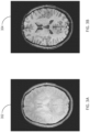
- FIGS. 3A and 3B two MR images of a brain corresponding to two different FAs are shown.
- FIG. 3A shows an image 302 of MR data acquired using a FA equal to 6°
- FIG. 3B shows an image 304 of MR data acquired using a FA equal to 24°.
- the repetition time TR used in acquiring the MR data illustrated in FIGS. 3A and 3B is equal to 25 milliseconds (ms).
- the values of the FAs associated with the images in FIGS. 3A and 3B are chosen for illustrative purposes and are not to be interpreted as limiting.
- angle values can be used for MR data acquisition given that the low FA (among the two FAs) is less than the Ernst angle and the large FA is greater than the Ernst angle.
- the processor 104 can reconstruct the images shown in FIGS. 3A and 3B by taking the inverse Fourier transform of the recorded signals associated with the corresponding FAs, respectively.
- the method 200 includes generating an apparent longitudinal relaxation time (T 1app ) map using the first MR dataset, the second MR dataset, and a constant value for a transmit RF field B 1t within the anatomical region (step 204).
- the T 1app map represents a spatial distribution of T 1app within the anatomical region.
- T 1app can be spatially varying even within a region associated with a single tissue due to the spatial inhomogeneity of B 1t .
- T 1app values can have a relatively large variance within a region representing one tissue. If there is a standard B 1t available for all people, then that can be used to find local T 1 values from person to person.
- Generating the T 1app map (step 204) can be viewed as determining a first estimate of the T 1app map to be used to reconstruct the B 1t map.
- the processor 104 can calculate T 1app on a pixel-by-pixel basis using equation (2) and assuming a normalized constant value for B 1t , e.g., equal to 1, within the anatomical region. Specifically, the processor 104 can first determine E1 for each pixel as the slope in equation (2) of a line defined based on the data points associated with the different FAs.
- E1 S ⁇ 1 sin B 1 t ⁇ 1 ⁇ S ⁇ 2 sin B 1 t ⁇ 2 / S ⁇ 1 tan B 1 t ⁇ 1 ⁇ S ⁇ 2 tan B 1 t ⁇ 2 .
- the processor 104 can then compute T 1app for each pixel according to equation (5) using the estimated value of T 1 and the constant value of B 1t , and therefore generate the T 1app map. Referring to FIG.
- FIG. 4A an image 402 of the T 1app map is depicted.
- the T 1app map shown in FIG. 4A is computed as described above on a pixel by pixel basis using the MR data shown in FIGS. 3A and 3B and a normalized constant value of B 1t equal to 1.
- the MR data is acquired using a value of TR equal to 25 ms.
- the method 200 includes the processor 104 estimating a first transmit RF field map by scaling the T 1app map by a first constant value of T 1 (step 206), and estimating a second transmit RF field map by scaling the T 1app map by a second constant value of T 1 (step 208).
- the first constant value of T 1 corresponds to a first tissue type within the anatomical region and the second constant value of T 1 corresponds to a second tissue type within the anatomical region.
- the first tissue type can be white matter and the second tissue type can be gray matter.
- 3D three-dimensional
- T 1 can be influenced by many factors, such as temperature, chemical exchange and perfusion.
- T 1 values for both gray matter and white matter recorded by various researchers show substantial variations. However, despite such variations, the ratio of T 1 values for gray matter divided by T 1 values for white matter appears fairly stable across various measurements by different researchers. Specifically, the ratio is about 1.7. Accordingly, the first constant value of T 1 can be set to 1000 ms, whereas the second constant value of T 1 can be set to 1700 ms. In some implementations, other values of T 1 for the white matter and gray matter can be selected. For example, the T 1 value for the white matter can be set to any value in the range of 800 to 1200 ms, and the T 1 value for the gray matter can be set to be equal 1.7 times the T 1 value for the whit matter. Also, for other types of tissue (e.g., other than gray matter and/or white matter), different T 1 values can be used.
- the processor 104 can generate the first estimate of the B 1t map by scaling (or dividing) the T 1app value at each pixel by the first constant value of T 1 .
- an image 404 of the first estimate of the B 1t map generated using the T 1app map shown in FIG. 4A is computed using a constant value of T 1 equal to 1000 ms and corresponding to white matter.
- the processor 104 can generate the second estimate of the B 1t map by scaling (or dividing) the T 1app value at each pixel by the second constant value of T 1 .
- the processor 104 can also generate masks for the first issue type and the second issue type within the anatomical region using at least one of the first estimate and the second estimate of the B 1t map. For instance, the processor 104 can use the first estimate of the B 1t map determined using a constant value of T 1 corresponding to white matter to generate a mask of white matter and a mask of gray matter.
- the estimates of the B 1t map are characterized by low spatial frequency content and can be adequate for segmenting the anatomical region into various regions corresponding to different tissue types.
- the processor 104 can apply a high-pass filter to the first estimate of the B 1t map to distinguish between white matter and gray matter regions.
- the processor 104 may apply a low-pass filter to the first estimate of the B 1t map to determine the white matter region, and apply a high-pass filter to the first estimate of the B 1t map to determine the gray matter region.
- the processor 104 can also apply an erosion algorithm to each mask to avoid interference or overlap between regions associated with different tissue types. For each of the masks generated by the processor 104, pixels associated with the corresponding tissue type can have a value equal to 1 (or a non-zero value) whereas other pixels can have a value equal to zero.
- FIGS. 5A and 5B images representing masks for white matter and gray matter are shown.
- the image 502 represents a mask of the white matter
- the image 504 represents a mask of the gray matter. Both masks are generated using the first estimate of the B 1t map shown in FIG. 4B .
- the processor 104 generates a third B 1t map using the estimated first B 1t and the estimated second B 1t map.
- FIG. 6A plots of the first estimate of B 1t and the second estimate of B 1t across a line within the anatomical region are shown.
- the plot 602 represents the first estimate of B 1t (or an estimate of B 1t using a constant value of T 1 corresponding to white matter) across the line within the anatomical region.
- the plot 604 represents the second estimate of B 1t (or an estimate of B 1t using a constant value of T 1 corresponding to gray matter) across the line within the anatomical region.
- Generating the third B 1t map can include the processor 104 shifting at least one of the first and second estimated maps of B 1t until both the first and second estimated maps of B 1t substantially overlap.
- the processor 104 can shift the first estimated map of B 1t by a shift value such that the mean square error between the shifted first estimated map of B 1t and the second estimated map of B 1t is minimized.
- the processor 104 can generate the third B 1t map using the shifted first estimated map of B 1t , the second estimated map of B 1t , and the masks corresponding to the first and second tissue types.
- the processor can (i) multiply (i.e., pixel by pixel multiplication) the mask corresponding to the first tissue type (e.g., white matter) with the shifted first estimated map of B 1t , (ii) multiply (i.e., pixel by pixel multiplication) the mask corresponding to the second tissue type (e.g., gray matter) with the second estimated map of B 1t , and (iii) merge the results of these multiplications to form a merged map of B 1t (or the third B 1t map).
- the processor 104 may apply local quadratic fitting to the merged map of B 1t (or the third B 1t map) to fill in (or assign values to) any pixels that do not belong to any of the generated masks.
- plots associated with the merged B 1t map with and without local quadratic fitting are depicted.
- the plot 606 represents values of the merged B 1t across a line within the anatomical region.
- the plot 608 represents the same values of the merged B 1t across the line within the anatomical region after applying local quadratic fitting.
- Local quadratic fitting can be achieved using a local quadratic fitting matrix of size m x m, where m is an integer. is used to create a smooth less noisy result throughout the entire n x n image. As illustrated in FIG. 6B , the local quadratic fitting operation leads to a smooth and less noise map of B 1t .
- an image 702 illustrating an example merged B 1t map is shown.
- the image 702 represents the resulting image when merging the multiplicative product of the mask 502 corresponding to the white matter and the shifted first estimated map of B 1t and the multiplicative product of the mask 504 corresponding to the gray matter and the second estimated map of B 1t .
- the black regions in the image 702 represent pixels or regions that belong neither to mask 502 nor to mask 504.
- an image 704 of B 1t map obtained after applying local quadratic fitting to image 702 is shown.
- the local quadratic fitting allows for filling in the gaps in the merged B 1t shown in FIG. 702.
- the B 1t map shown in image 704 provides a reliable estimate of B 1t within the anatomical region and allows for accurate reconstruction of the T 1 map and/or the SD map.
- the anatomical region can include more than two different tissue types.
- the anatomical region can include three distinct tissue types.
- the processor 104 can further determine another estimate of the B 1t map by scaling the T 1app map (generated at step 204) by a third constant value of T 1 associated with the third tissue type within the anatomical region.
- the processor 104 can also generate a third mask representative of the region occupied by the third tissue type within the anatomical region.
- the processor 104 can use different filters (e.g., low-pass filter(s), band-pass filter(s), and/or a high-pass filter(s)) to generate each of the three masks.
- the processor 104 can update the third B 1t map using the map of B 1t estimated based on the third constant value of T 1 (e.g., according to the third mask). Alternatively, the processor 104 can (initially) generate the third B 1t map using the three estimates of the B 1t map (e.g., based on the three masks corresponding to the three tissue types).
- the third tissue type can be cerebro-spinal fluid and the processor 104 can (i) multiply the first B 1t map estimated based the constant T 1 value for white matter by the first mask, (ii) multiply the second B 1t map estimated using the constant T 1 value for gray matter by the second mask, (iii) multiply the B 1t map estimated using the constant T 1 value for cerebro-spinal fluid by the third mask, and (iv) so on for other tissues.
- the constant T 1 value for cerebro-spinal fluid can be equal to 4500 ms.
- the processor 104 can then merge the resulting images (from the multiplications with masks) to create a single more accurate B 1t map image.
- the processor 104 may remove local noise spikes by using, for example, a sliding window to calculate the mean and standard deviation in the window and remove those points (or pixels) that lie beyond a given threshold value (e.g., three standard deviations of the noise) above or below the mean.
- the processor 104 can apply local quadratic fitting as described above with regard to FIG. 6B to the merged B 1t map using, for example, a local quadratic fitting matrix of size m x m to provide a smooth and less noisy B 1t map image, where m is an integer.
- the integer m can be equal to 20. However, other values for m may be used.
- tissue types can include white matter, gray matter, and cerebro-spinal fluid
- the methods and systems are to be interpreted as limited to the human brain or to these tissue types.
- the methods described herein are not to be restricted to a specific anatomical region or to a specific number of tissue types within the anatomical region.
- the method 200 can further include the processor 104 using the B 1t map determined at step 210 to generate a first estimate of the T 1 map.
- the processor 104 can generate a map of SD eff by dividing the value corresponding to the intersection with the x-axis by 1 - E 1 at each pixel, and multiply the SDeff map by the constant value of B 1t assumed at step 204 to generate the SD app map.
- the processor 104 can generate a first estimate of the SD map by dividing the determined SD app map by the B 1t map determined at step 210. According to Equation (4), for each pixel or voxel within the anatomical region, the processor 104 can scale (or divide) the SD app value at that pixel by the B 1t value at the same pixel (from the B 1t map generated at step 210).
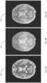
- images 802, 804 and 806 illustrate examples of an estimate of a T 1 map, an estimate of a SD app map, and an estimate of a SD map, respectively.
- the T 1 map shown in image 802 is generated by scaling (on a pixel by pixel basis) the T 1app map in in image 402 (shown in FIG. 4A ) by the square of B 1t shown in image 704 ( FIG. 7B ).
- the estimate of the SD app map in image 804 is generated using Equation (3), one of the datasets illustrated in images 302 or 304 ( FIGS. 3A and 3B ).
- the estimate of the SD map (or SD eff map) of image 806 is generated by dividing the SD app map of image 704 by the B 1t map of image 704 ( FIG. 7B ).
- the processor 104 can use the estimated B 1t map (determined at step 210), the corrected T 1 map and the corrected SD map to estimate (or generate) a map of B 1r .
- the processor 104 can employ the estimated B 1t map as well as the corrected T 1 and SD maps to synthesize a MR dataset corresponding to a specific flip angle that can make a first region associated with a first tissue type (e.g., white matter) and a second region associated with a second tissue type (e.g., gray matter) isointense.
- the processor 104 can synthesize such a MR dataset without additional MR data acquisition via the MRI scanner 102, but rather by using Equation (1).
- the processor 104 may further vary the echo time TE to create a MR dataset where three regions corresponding to three different tissue types (e.g., white matter, gray matter, and cerebro-spinal fluid) are isointense.
- the processor 104 can scale the SD map estimate (e.g., the SD map shown in image 806 of FIG. 8C ) by the estimated B 1r map to alleviate the effect of the spatial variation of B 1r within the anatomical region and achieve an improved estimate of the SD map.
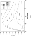
- example signals corresponding to different tissue types over a range of FAs are shown.
- the signal 902 corresponds to white matter (or WM)
- signal 904 corresponds to gray matter (or GM)
- signal 906 corresponds to cerebro-spinal fluid (or CSF).
- the signal 908 represents the difference between signals 902 and 904
- the signal 910 represents the difference between signals 904 and 906,
- the signal 912 represents the difference between signals 902 and 906.
- the signals 902, 904, and 906 were generated using constant T 1 values equal to 1000 ms within white matter, 1700 ms within gray matter, and 4500 ms within cerebro-spinal fluid.
- the repetition time TR is equal to 30 ms
- the white matter SD is equal to 0.68
- the SD of gray matter is equal to 0.82.
- the T 2 * values of 44 ms and 51 ms were used for white matter and gray matter, respectively.
- signals 902 and 904 intersect at a FA about (or slightly above) 10°.
- the processor 104 can avoid the need to determine the local spin density. Since all signals are isointense, the amplitude variation in the synthesized dataset represents the variation in the B 1r field. Accordingly, the processor 104 can determine (or generate) a B 1r map based on the synthesized data set.
- the processor 104 may also employ local quadratic fitting in estimating the B 1r map.
- the B 1r map used to correct the initial images can be defined as the signal from the isointense image normalized to the value of B 1r in the center of the image.
- Image 1002 represents a double isointense MR dataset where the FA is selected such that the white matter and the gray matter are isointense.
- the image 1004 represents a B 1r map generated (or estimated) based on the isointense MR dataset of image 1002.
- the isointense MR dataset in image 1002 includes gaps (black regions or pixels). Such gaps are eliminated in the B 1r map of image 1004 by using local quadratic fitting.
- the processor 104 may scale the SD map estimate (e.g., the SD map shown in image 806 of FIG.
- the image 1006 represents a scaling (pixel-by-pixel scaling) of the SD map in image 806 by the B 1r map of image 1004. Comparing the images 1006 and 806, one can see that the SD map in image 1006 provides an improved representation of the various sub-regions within the anatomical region compared to image 806.
- the processor 104 can estimate a plurality of B 1t maps for a plurality of subjects (e.g., patients or volunteers).
- the processor 104 may estimate the B 1t map for each subject as described above with regard to method 200.
- the processor 104 can transform the corresponding B 1t map for each subject into a respective template of the anatomical region (e.g., brain).
- the processor 104 can accomplish this by first transforming the magnitude image of the first dataset into a template brain (e.g., using Insight Segmentation, and Registration Toolkit (ITK)).
- ITK Insight Segmentation, and Registration Toolkit
- the processor 104 can then average the B 1t values in the templates associated with the plurality of subjects into a common B 1t template.
- the averaging can be a weighted averaging. For example, some templates associated with some subjects may be weighted more or less than other templates.
- the processor 104 can use the common (or average) B 1t template as an estimate of the B 1t map for various patients by performing an inverse transform back to the patient space.
- the common (or average) B 1t template can be computed offline and used in reconstructing T 1 maps or SD maps (as described above with regard to the B 1t map generated at step 201) for various patients.
- the processor 104 may avoid generating a B 1t map for each new scanned subject and instead use the pre-computed common (or average) B 1t template.
- the processor can use both the precomputed common (or average) B 1t template and an estimate of the B 1t map specific to the patient to generate separate images of the anatomical region (e.g., separate images of the T 1 map).
- the common (or average) B 1r template can be computed offline, and the processor 104 can use the common (or average) B 1r template as an estimate of the B 1r map for various patients.
- the availability of a precomputed common (or average) B 1r template can allow avoiding the construction (or computation) of a respective B 1r map for each newly scanned patient.
- the processor can use both the precomputed common (or average) B 1r template and an estimate of the B 1r map specific to the patient to generate separate images of the anatomical region.
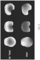
- Examples of brain templates for the B 1t and B 1r map are shown.
- the upper row of images illustrates an example common (or average) brain template for the B 1t map.
- This common (or average) template represents an estimate of the B 1t map that can be used for various subjects.
- the lower row of images illustrates an example common (or average) brain template for the B 1r map.
- This common (or average) template represents an estimate of the B 1r map that can be used for various subjects.
- the processor 104 can inverse transform the average B 1t template (e.g., using ITK) and/or the average B 1r template for that specific subject. For instance, the processor can adjust the common (or average) B 1t template and/or the common (or average) B 1r template to conform with the size of the anatomical region (e.g., brain) for a specific patient. The processor 104 may use the inverse transformed common (or average) B 1t template to estimate the T 1 map for that specific patient.
- the processor 104 can scale (or divide on a pixel-by-pixel or voxel-by-voxel basis) the T 1app map for the patient by the square of the inverse transformed common (or average) B 1t template to generate an estimate of the T 1 map.
- Such estimate can either substitute the estimate based on an estimated B 1t map specific to the patient or can be an additional (or second) estimate of the T 1 map.
- the processor 104 may also use the common (or average) B 1t when estimating the SD (or SD eff ) map for the patient.
- the processor 104 may scale (or divide on a pixel-by-pixel or voxel-by-voxel basis) the SD app map for the patient by the inverse transformed common (or average) B 1t template to generate an estimate of the SD map.
- the processor 104 can also scale the original datasets (corresponding to FAs ⁇ 1 and ⁇ 2 ) acquired at step 202 by the B 1r map estimated based on the synthesized dataset, and generate a MR image of the anatomical region by subtracting the scaled datasets.
- the generated MR image can illustrate the various tissue types within the anatomical regions based on the respective T 1 values.
- the processor 104 can employ a weighted subtraction when subtracting a first scaled MR dataset corresponding to the first FA from the other scaled dataset corresponding to the second FA.
- the processor 104 can scale the original datasets (corresponding to FAs ⁇ 1 and ⁇ 2 ) acquired at step 202 by the common (or average) B 1r template computed or reconstructed offline (or an inverse transformation thereof). In some implementations, the processor 104 may scale the SD map estimate (e.g., the SD map shown in image 806 of FIG. 8C ) by the common (or average) B 1r template to alleviate the effect of the spatial variation of B 1r within the anatomical region on the estimated SD map.
- the SD map estimate e.g., the SD map shown in image 806 of FIG. 8C
- the processor 104 can subtract (without scaling) images corresponding to the original datasets (corresponding to FAs ⁇ 1 and ⁇ 2 ) acquired at step 202 to generate another (or an alternative) MR image of the anatomical region.
- Such MR images can illustrate the various tissue types within the anatomical regions based on the respective T 1 values.
- Images 1202 and 1204 represent scalings of images 302 and 304, respectively, by the B 1r map in image 1002.
- the images 1202 and 1204 represent an improvement over the corresponding original images 302 and 304 since the scaling by the B 1r map alleviates the effect of the spatial variation of B 1r within the anatomical region.
- images 1202 and 1204 still suffer from the effect of the spatial variation of B 1t within the anatomical region.
- the image 1206 represents a subtraction between the images 302 and 304 (e.g., subtracting the image corresponding to the low FA from the image corresponding to the large FA) corresponding to the original acquired datasets for the two FAs.
- the image 1208 represents a subtraction between the scaled images 1202 and 1204 (e.g., subtracting the image corresponding to the low FA from the image corresponding to the large FA). While both images 1206 and 1208 provide an improved representation of the various tissues within the anatomical region compared to the images 302 and 304 corresponding to the original acquired data, the image 1208 represents an improvement over image 1206 since the effect of the spatial variation of B 1r within the anatomical region is eliminated (or alleviated) in the former image 1208.
- the methods and system described herein provide various techniques for generating improved images of anatomical regions scanned using two flip angles. These methods and system are not to be interpreted as limited to human brain and can be used for other anatomical regions. Also, while this disclosure describes various techniques described for generating various MR images (e.g., of the estimated T 1 map, the estimated SD map, the scaled SD map, the subtraction MR image, the scaled subtraction MR image, the estimated B 1t map, the estimated B 1r map, the common B 1t template, or the common B 1r template), this disclosure should be interpreted as encompassing various combinations of such techniques or corresponding MR images. Furthermore, the process 104 can apply the techniques for generating various MR images described herein for multiple echo times.
- the processor 104 can apply averaging or weighted averaging to MR images (e.g., B 1t maps, B 1r maps, T 1app maps, T 1 maps, SD app maps, SD maps, etc.) generated based on datasets associated with the various echo times to provide improved images of anatomical regions.
- MR images e.g., B 1t maps, B 1r maps, T 1app maps, T 1 maps, SD app maps, SD maps, etc.
- processes described in this disclosure can be implemented using computer code instructions executable by a processor.
- the computer code instructions can be stored on a non-transitory or tangible computer-readable medium such as a random access memory (RAM), a read only memory (ROM), a cache memory, a disc memory, any other memory, or any other computer readable medium.
- Processes described in this disclosure can be implemented by an apparatus including at least one processor and/or memory storing executable code instructions.
- the code instructions when executed by the at least one processor can cause performing at least one of the processes or operations described in this disclosure.
- the apparatus can for example be a MRI scanner, a computer device or other electronic device associated with a MRI scanner.
Landscapes
- Physics & Mathematics (AREA)
- Health & Medical Sciences (AREA)
- Engineering & Computer Science (AREA)
- Life Sciences & Earth Sciences (AREA)
- Nuclear Medicine, Radiotherapy & Molecular Imaging (AREA)
- High Energy & Nuclear Physics (AREA)
- General Health & Medical Sciences (AREA)
- Radiology & Medical Imaging (AREA)
- General Physics & Mathematics (AREA)
- Condensed Matter Physics & Semiconductors (AREA)
- Signal Processing (AREA)
- Biophysics (AREA)
- Public Health (AREA)
- Surgery (AREA)
- Animal Behavior & Ethology (AREA)
- Molecular Biology (AREA)
- Medical Informatics (AREA)
- Veterinary Medicine (AREA)
- Heart & Thoracic Surgery (AREA)
- Biomedical Technology (AREA)
- Pathology (AREA)
- Artificial Intelligence (AREA)
- Physiology (AREA)
- Computer Vision & Pattern Recognition (AREA)
- Psychiatry (AREA)
- Cardiology (AREA)
- Power Engineering (AREA)
- Pulmonology (AREA)
- Neurology (AREA)
- Evolutionary Computation (AREA)
- Fuzzy Systems (AREA)
- Mathematical Physics (AREA)
- Magnetic Resonance Imaging Apparatus (AREA)
Claims (13)
- Procédé d'imagerie par résonance magnétique (IRM), comprenant :la réception (202), par au moins un processeur (104), d'un premier ensemble de données d'écho de gradient de résonance magnétique (RM) correspondant à un premier angle de bascule et à une première séquence RM d'écho de gradient rapide avec spoiler et un deuxième ensemble de données d'écho de gradient RM correspondant à un deuxième angle de bascule et à une deuxième séquence RM d'écho de gradient rapide avec spoiler, le premier ensemble de données d'écho de gradient RM et le deuxième ensemble de données d'écho de gradient RM acquis par imagerie d'une région anatomique en utilisant au moins un temps d'écho, le premier angle de bascule étant différent du deuxième angle de bascule ;la génération (204), par au moins un processeur (104), d'une carte de temps de relaxation longitudinale apparente (T1app), représentant une distribution spatiale de T1app dans la région anatomique en utilisant le premier ensemble de données d'écho de gradient RM, le deuxième ensemble de données d'écho de gradient RM et une valeur constante pour un champ de radiofréquence (RF) d'émission dans la région anatomique ;l'estimation (206), par l'au moins un processeur (104), d'une première carte de champ RF d'émission en mettant à l'échelle la carte T1app par une première valeur constante de temps de relaxation longitudinale (T1), la première valeur constante de T1 étant associée à un premier type de tissu dans la région anatomique ;l'estimation (208), par l'au moins un processeur (104), d'une deuxième carte de champ RF d'émission en mettant à l'échelle la carte T1app par une deuxième valeur constante de T1, la deuxième valeur constante de T1 étant associée à un deuxième type de tissu dans la région anatomique ; etla génération (210), par l'au moins un processeur (104), d'une troisième carte de champ RF d'émission en utilisant une première région de la première carte de champ RF d'émission estimée correspondant au premier type de tissu dans la région anatomique et une deuxième région de la deuxième carte de champ RF d'émission estimée correspondant au deuxième type de tissu dans la région anatomique, la troisième carte de champ RF d'émission représentant une distribution spatiale du champ RF d'émission dans la région anatomique.
- Procédé selon la revendication 1, dans lequel la région anatomique est un cerveau humain, le premier type de tissu est la matière blanche, et le deuxième type de tissu est la matière grise.
- Procédé selon la revendication 1 comprenant en outre :l'estimation, par l'au moins un processeur, d'une quatrième carte de champ RF d'émission en mettant à l'échelle la carte T1app par une troisième valeur constante de T1, la troisième valeur constante de T1 étant associée à un troisième type de tissu dans la région anatomique,dans lequel la génération de la troisième carte de champ RF d'émission inclut l'utilisation de la première carte de champ RF d'émission estimée, de la deuxième carte de champ RF d'émission estimée et de la quatrième carte de champ RF d'émission estimée.
- Procédé selon la revendication 3, dans lequel la région anatomique est un cerveau humain, le premier type de tissu est la matière blanche, le deuxième type de tissu est la matière grise et le troisième type de tissu est le liquide cérébro-spinal.
- Procédé selon la revendication 1 comprenant en outre :
la génération, par l'au moins un processeur, d'une première carte de temps de relaxation longitudinale (T1) en divisant la carte T1app par le carré de la troisième carte de champ RF d'émission, la première carte T1 représentant une distribution spatiale de T1 au sein de la région anatomique. - Procédé selon la revendication 5 comprenant en outre :la génération, par l'au moins un processeur, d'une carte de densité apparente de spin (SDapp) en utilisant le premier ensemble de données d'écho de gradient RM, le deuxième ensemble de données d'écho de gradient RM et la valeur constante du champ RF d'émission, la carte SDapp représentant une distribution spatiale de SDapp dans la région anatomique ; etla génération, par l'au moins un processeur, d'une première carte de densité de spin (SD) en mettant à l'échelle la carte SDapp par la troisième carte de champ RF d'émission ;la synthèse, par l'au moins un processeur, en utilisant la troisième carte de champ RF, la première carte T1 et la première carte SD, d'un troisième ensemble de données d'écho de gradient RM correspondant à un troisième angle de bascule de sorte qu'au moins une première sous-région de la région anatomique correspondant au premier type de tissu et une deuxième sous-région de la région anatomique correspondant au deuxième type de tissu soient iso-intenses ;l'estimation, par l'au moins un processeur, d'une carte de champ RF de réception en utilisant le troisième ensemble de données d'écho de gradient MR synthétisé, la carte de champ RF de réception représentant une distribution spatiale d'un champ RF de réception dans la région anatomique ; etla génération, par l'au moins un processeur, d'une deuxième carte SD en mettant à l'échelle la première carte SD avec la carte estimée du champ RF de réception.
- Procédé selon la revendication 1 comprenant en outre :l'estimation, par l'au moins un processeur, d'une pluralité de cartes de champ RF d'émission pour une pluralité de sujets ; etla génération, par l'au moins un processeur, d'un modèle de champ RF d'émission en utilisant une moyenne de la pluralité estimée de cartes de champ RF d'émission pour la pluralité de sujets.
- Procédé selon la revendication 7 comprenant en outre :
la génération, par l'au moins un processeur, d'une carte de densité de spin (SD) en utilisant une carte SDapp estimée, le modèle de champ RF de transmission et une carte de champ RF de réception estimée. - Procédé selon la revendication 7 comprenant en outre :
la génération, par l'au moins un processeur, d'une deuxième carte T1 en utilisant la carte T1app et le modèle de champ RF d'émission. - Procédé selon la revendication 6 comprenant en outre :la mise à l'échelle, par l'au moins un processeur, du premier ensemble de données d'écho de gradient MR par la carte de champ RF de réception ;la mise à l'échelle, par l'au moins un processeur, du deuxième ensemble de données d'écho de gradient MR par la carte de champ RF de réception ; etla génération, par l'au moins un processeur, d'une image représentant une soustraction pondérée de l'ensemble de données du premier écho de gradient RM mis à l'échelle et de l'ensemble de données du deuxième écho de gradient RM mis à l'échelle.
- Procédé selon la revendication 1 comprenant en outre la génération d'une image représentant une soustraction pondérée du premier ensemble de données d'écho de gradient RM du deuxième ensemble de données d'écho de gradient RM.
- Support non transitoire lisible par ordinateur comprenant des instructions de code informatique stockées sur celui-ci, les instructions de code informatique, lorsqu'elles sont exécutées par au moins un processeur, amènent l'au moins un processeur à mettre en oeuvre un procédé selon l'une quelconque des revendications 1 à 11.
- Système d'imagerie par résonance magnétique (IRM) comprenant :un scanner IRM (102) configuré pour acquérir le premier ensemble de données d'écho de gradient de résonance magnétique (RM) correspondant à un premier angle de bascule et le deuxième ensemble de données d'écho de gradient de RM correspondant à un deuxième angle de bascule par imagerie d'une région anatomique en utilisant au moins un temps d'écho ;au moins un processeur (104) ; etune mémoire (106), comportant des instructions de code informatique stockées en son sein, les instructions de code informatique, lorsqu'elles sont exécutées par l'au moins un processeur, amènent l'au moins un processeur à réaliser un procédé selon l'une quelconque des revendications 1 à 11.
Applications Claiming Priority (2)
| Application Number | Priority Date | Filing Date | Title |
|---|---|---|---|
| US15/659,353 US10451697B2 (en) | 2017-07-25 | 2017-07-25 | Systems and methods for strategically acquired gradient echo imaging |
| PCT/US2017/043991 WO2019022733A1 (fr) | 2017-07-25 | 2017-07-26 | Systèmes et procédés d'imagerie en écho de gradient acquise de façon stratégique |
Publications (4)
| Publication Number | Publication Date |
|---|---|
| EP3658018A1 EP3658018A1 (fr) | 2020-06-03 |
| EP3658018A4 EP3658018A4 (fr) | 2021-04-07 |
| EP3658018B1 true EP3658018B1 (fr) | 2025-02-19 |
| EP3658018C0 EP3658018C0 (fr) | 2025-02-19 |
Family
ID=65037799
Family Applications (1)
| Application Number | Title | Priority Date | Filing Date |
|---|---|---|---|
| EP17918854.5A Active EP3658018B1 (fr) | 2017-07-25 | 2017-07-26 | Systèmes et procédés d'imagerie en écho de gradient acquise de façon stratégique |
Country Status (6)
| Country | Link |
|---|---|
| US (1) | US10451697B2 (fr) |
| EP (1) | EP3658018B1 (fr) |
| JP (1) | JP6872079B2 (fr) |
| KR (1) | KR102353790B1 (fr) |
| CN (1) | CN111065328B (fr) |
| WO (1) | WO2019022733A1 (fr) |
Families Citing this family (9)
| Publication number | Priority date | Publication date | Assignee | Title |
|---|---|---|---|---|
| WO2020123788A1 (fr) * | 2018-12-14 | 2020-06-18 | The Board Of Trustees Of The Leland Stanford Junior University | Irm qualitative et quantitative utilisant un apprentissage profond |
| US11119170B1 (en) | 2020-06-11 | 2021-09-14 | Spintech, Inc. | Systems and methods for enhancement of resolution for strategically acquired gradient echo (STAGE) imaging |
| US11249159B2 (en) | 2020-06-11 | 2022-02-15 | Spintech, Inc. | Systems and methods for enhancement of resolution for strategically acquired gradient echo (stage) imaging |
| KR20230164161A (ko) * | 2021-04-02 | 2023-12-01 | 스핀테크, 인크. | 해부학적 구조의 템플릿 기반 자동 검출을 위한 시스템 및 방법 |
| US11435424B1 (en) * | 2021-08-27 | 2022-09-06 | Spintech, Inc. | Systems and methods of constrained reconstruction of images with white noise |
| KR102782813B1 (ko) * | 2022-06-07 | 2025-03-19 | 가천대학교 산학협력단 | 자기공명영상의 뇌 분할 시스템 및 방법 |
| JP2023180392A (ja) * | 2022-06-09 | 2023-12-21 | キヤノンメディカルシステムズ株式会社 | 磁気共鳴イメージング装置、位相補正方法、および撮像制御方法 |
| CN115184852B (zh) * | 2022-07-18 | 2025-07-25 | 沈阳工业大学 | 一种磁共振成像的方法及系统 |
| CN118105055A (zh) * | 2022-11-30 | 2024-05-31 | 西门子(深圳)磁共振有限公司 | 确定多组织磁共振扫描的翻转角的方法及装置 |
Family Cites Families (19)
| Publication number | Priority date | Publication date | Assignee | Title |
|---|---|---|---|---|
| US6603989B1 (en) | 2000-03-21 | 2003-08-05 | Dmitriy A. Yablonskiy | T2 contrast in magnetic resonance imaging with gradient echoes |
| US6819952B2 (en) * | 2001-03-23 | 2004-11-16 | The Board Of Trustees Of The Leland Stanford Junior University | Magnetic resonance spectroscopic imaging method to monitor progression and treatment of neurodegenerative conditions |
| DE102006018413A1 (de) * | 2006-04-20 | 2007-10-25 | Siemens Ag | MR-Tomograph mit einem System zur Kontrastoptimierung von MRT-Bildern |
| GB0619269D0 (en) | 2006-09-29 | 2006-11-08 | King S College London | Method of mapping a magnetic field for use in magnetic resonance imaging |
| CN101981462B (zh) * | 2008-03-27 | 2014-12-24 | 皇家飞利浦电子股份有限公司 | 具有针对多rf发射系统的改进的b1映射的翻转角成像 |
| EP2141506B1 (fr) * | 2008-07-01 | 2019-04-03 | The Regents of The University of California | Identification de trajets de fibres par imagerie à résonance magnétique (IRM) |
| US8502538B2 (en) | 2009-03-19 | 2013-08-06 | Kabushiki Kaisha Toshiba | B1 and/or B0 mapping in MRI system using k-space spatial frequency domain filtering with complex pixel by pixel off-resonance phase in the B0 map |
| US9271651B2 (en) * | 2009-11-30 | 2016-03-01 | General Electric Company | System and method for integrated quantifiable detection, diagnosis and monitoring of disease using patient related time trend data |
| DE102010020770A1 (de) * | 2010-05-17 | 2011-11-17 | Siemens Aktiengesellschaft | Verfahren zur Reduzierung von Bildartefakten, insbesondere von Metallartefakten, in CT-Bilddaten |
| WO2012060192A1 (fr) | 2010-11-05 | 2012-05-10 | 株式会社 日立メディコ | Dispositif d'imagerie par résonance magnétique et procédé de mesure du champ magnétique d'irradiation |
| US9002428B2 (en) * | 2011-01-28 | 2015-04-07 | The Board Of Trustees Of The Leland Stanford Junior University | Methods for detecting abnormalities and degenerative processes in soft tissue using magnetic resonance imaging (MRI) |
| US9921283B2 (en) * | 2011-01-28 | 2018-03-20 | The Board Of Trustees Of The Leland Stanford Junior University | Methods for detecting abnormalities and degenerative processes in soft tissue using magnetic resonance imaging |
| US9201158B2 (en) * | 2012-01-24 | 2015-12-01 | Schlumberger Technology Corporation | Estimating and displaying molecular size information of a substance |
| US9625547B2 (en) | 2013-03-28 | 2017-04-18 | Universitatsspital Basel | Magnetic resonance imaging method for the quantification of the T1 and/or T2 relaxation times in a sample |
| CN104856676B (zh) * | 2014-02-26 | 2017-10-03 | 西门子(深圳)磁共振有限公司 | 磁共振成像方法和装置 |
| US9530219B2 (en) * | 2014-07-02 | 2016-12-27 | Covidien Lp | System and method for detecting trachea |
| US10598750B2 (en) * | 2015-04-02 | 2020-03-24 | The General Hospital Corporation | 3D balanced EPI magnetic resonance fingerprinting |
| WO2017022136A1 (fr) * | 2015-08-06 | 2017-02-09 | 株式会社日立製作所 | Dispositif d'imagerie par résonance magnétique |
| WO2017053799A1 (fr) | 2015-09-25 | 2017-03-30 | Oregon Health & Science University | Systèmes et procédés pour l'imagerie fonctionnelle du placenta |
-
2017
- 2017-07-25 US US15/659,353 patent/US10451697B2/en active Active
- 2017-07-26 JP JP2020527724A patent/JP6872079B2/ja active Active
- 2017-07-26 CN CN201780094537.0A patent/CN111065328B/zh active Active
- 2017-07-26 KR KR1020207005227A patent/KR102353790B1/ko active Active
- 2017-07-26 EP EP17918854.5A patent/EP3658018B1/fr active Active
- 2017-07-26 WO PCT/US2017/043991 patent/WO2019022733A1/fr not_active Ceased
Non-Patent Citations (1)
| Title |
|---|
| WEISKOPF N ET AL: "Unified segmentation based correction of R1 brain maps for RF transmit field inhomogeneities (UNICORT)", NEUROIMAGE, ELSEVIER, AMSTERDAM, NL, vol. 54, no. 3, 1 February 2011 (2011-02-01), pages 2116 - 2124, XP027564683, ISSN: 1053-8119, [retrieved on 20101217] * |
Also Published As
| Publication number | Publication date |
|---|---|
| CN111065328B (zh) | 2023-10-10 |
| CN111065328A (zh) | 2020-04-24 |
| JP2020530805A (ja) | 2020-10-29 |
| EP3658018A1 (fr) | 2020-06-03 |
| KR102353790B1 (ko) | 2022-01-19 |
| JP6872079B2 (ja) | 2021-05-19 |
| KR20200032167A (ko) | 2020-03-25 |
| WO2019022733A1 (fr) | 2019-01-31 |
| US10451697B2 (en) | 2019-10-22 |
| EP3658018C0 (fr) | 2025-02-19 |
| US20190033418A1 (en) | 2019-01-31 |
| EP3658018A4 (fr) | 2021-04-07 |
Similar Documents
| Publication | Publication Date | Title |
|---|---|---|
| EP3658018B1 (fr) | Systèmes et procédés d'imagerie en écho de gradient acquise de façon stratégique | |
| Marques et al. | Studying cyto and myeloarchitecture of the human cortex at ultra-high field with quantitative imaging: R1, R2* and magnetic susceptibility | |
| US9797974B2 (en) | Nonrigid motion correction in 3D using autofocusing with localized linear translations | |
| JP6085545B2 (ja) | 磁気共鳴イメージング装置、画像処理装置および磁化率画像算出方法 | |
| US10605883B2 (en) | System and method for producing distortion free magnetic resonance images using dual-echo echo-planar imaging | |
| US20090206838A1 (en) | Systems and Methods for Correction of Inhomogeneities in Magnetic Resonance Images | |
| US20150145514A1 (en) | System and method for object-based initialization of magnetic field inhomogeneity in magnetic resonance imaging | |
| US9733329B2 (en) | System and method for field map estimation | |
| US20140314293A1 (en) | System and method for joint degradation estimation and image reconstruction in magnetic resonance imaging | |
| US8995738B2 (en) | System and method for magnetic resonance imaging parametric mapping using confidence maps | |
| Chung et al. | An improved PSF mapping method for EPI distortion correction in human brain at ultra high field (7T) | |
| Nachmani et al. | The effect of motion correction interpolation on quantitative T1 mapping with MRI | |
| US11241163B2 (en) | Measuring blood vessel characteristics with MRI | |
| US11249159B2 (en) | Systems and methods for enhancement of resolution for strategically acquired gradient echo (stage) imaging | |
| US11467238B2 (en) | Method for uniform reconstruction of multi-channel surface-coil magnetic resonance data without use of a reference scan | |
| Park et al. | Development of a bias field-based uniformity correction in magnetic resonance imaging with various standard pulse sequences | |
| Zhao et al. | k-space weighted image average (KWIA) for ASL-based dynamic MR angiography and perfusion imaging | |
| HK40028698B (zh) | 用於有策略地获取的梯度回波成像的系统和方法 | |
| HK40028698A (en) | Systems and methods for strategically acquired gradient echo imaging | |
| Huang et al. | Physics-Informed Implicit Neural Representations for Joint B0 Estimation and Echo Planar Imaging | |
| US10132890B2 (en) | System and method for controlling undesired magnetic field effects in magnetic resonance imaging | |
| US11119170B1 (en) | Systems and methods for enhancement of resolution for strategically acquired gradient echo (STAGE) imaging | |
| JP6776217B2 (ja) | 画像処理装置、画像処理方法、画像処理プログラム及び磁気共鳴イメージング装置 | |
| Raja et al. | Extended neighbourhood based linear reconstruction of Diffusion Kurtosis Imaging | |
| Rohde et al. | Estimating intensity variance due to noise in registered images |
Legal Events
| Date | Code | Title | Description |
|---|---|---|---|
| STAA | Information on the status of an ep patent application or granted ep patent |
Free format text: STATUS: THE INTERNATIONAL PUBLICATION HAS BEEN MADE |
|
| PUAI | Public reference made under article 153(3) epc to a published international application that has entered the european phase |
Free format text: ORIGINAL CODE: 0009012 |
|
| STAA | Information on the status of an ep patent application or granted ep patent |
Free format text: STATUS: REQUEST FOR EXAMINATION WAS MADE |
|
| 17P | Request for examination filed |
Effective date: 20200224 |
|
| AK | Designated contracting states |
Kind code of ref document: A1 Designated state(s): AL AT BE BG CH CY CZ DE DK EE ES FI FR GB GR HR HU IE IS IT LI LT LU LV MC MK MT NL NO PL PT RO RS SE SI SK SM TR |
|
| AX | Request for extension of the european patent |
Extension state: BA ME |
|
| DAV | Request for validation of the european patent (deleted) | ||
| DAX | Request for extension of the european patent (deleted) | ||
| REG | Reference to a national code |
Ref country code: DE Ref legal event code: R079 Ref document number: 602017087945 Country of ref document: DE Free format text: PREVIOUS MAIN CLASS: A61B0005055000 Ipc: G01R0033500000 |
|
| A4 | Supplementary search report drawn up and despatched |
Effective date: 20210304 |
|
| RIC1 | Information provided on ipc code assigned before grant |
Ipc: G01R 33/50 20060101AFI20210301BHEP Ipc: G01R 33/24 20060101ALI20210301BHEP |
|
| STAA | Information on the status of an ep patent application or granted ep patent |
Free format text: STATUS: EXAMINATION IS IN PROGRESS |
|
| 17Q | First examination report despatched |
Effective date: 20230119 |
|
| GRAP | Despatch of communication of intention to grant a patent |
Free format text: ORIGINAL CODE: EPIDOSNIGR1 |
|
| STAA | Information on the status of an ep patent application or granted ep patent |
Free format text: STATUS: GRANT OF PATENT IS INTENDED |
|
| RIC1 | Information provided on ipc code assigned before grant |
Ipc: A61B 5/00 20060101ALN20240403BHEP Ipc: G01R 33/56 20060101ALI20240403BHEP Ipc: G01R 33/24 20060101ALI20240403BHEP Ipc: G01R 33/50 20060101AFI20240403BHEP |
|
| INTG | Intention to grant announced |
Effective date: 20240425 |
|
| GRAJ | Information related to disapproval of communication of intention to grant by the applicant or resumption of examination proceedings by the epo deleted |
Free format text: ORIGINAL CODE: EPIDOSDIGR1 |
|
| STAA | Information on the status of an ep patent application or granted ep patent |
Free format text: STATUS: EXAMINATION IS IN PROGRESS |
|
| GRAP | Despatch of communication of intention to grant a patent |
Free format text: ORIGINAL CODE: EPIDOSNIGR1 |
|
| STAA | Information on the status of an ep patent application or granted ep patent |
Free format text: STATUS: GRANT OF PATENT IS INTENDED |
|
| INTC | Intention to grant announced (deleted) | ||
| RIC1 | Information provided on ipc code assigned before grant |
Ipc: A61B 5/00 20060101ALN20240903BHEP Ipc: G01R 33/56 20060101ALI20240903BHEP Ipc: G01R 33/24 20060101ALI20240903BHEP Ipc: G01R 33/50 20060101AFI20240903BHEP |
|
| INTG | Intention to grant announced |
Effective date: 20240912 |
|
| GRAS | Grant fee paid |
Free format text: ORIGINAL CODE: EPIDOSNIGR3 |
|
| GRAA | (expected) grant |
Free format text: ORIGINAL CODE: 0009210 |
|
| STAA | Information on the status of an ep patent application or granted ep patent |
Free format text: STATUS: THE PATENT HAS BEEN GRANTED |
|
| AK | Designated contracting states |
Kind code of ref document: B1 Designated state(s): AL AT BE BG CH CY CZ DE DK EE ES FI FR GB GR HR HU IE IS IT LI LT LU LV MC MK MT NL NO PL PT RO RS SE SI SK SM TR |
|
| REG | Reference to a national code |
Ref country code: GB Ref legal event code: FG4D |
|
| REG | Reference to a national code |
Ref country code: CH Ref legal event code: EP |
|
| REG | Reference to a national code |
Ref country code: IE Ref legal event code: FG4D |
|
| REG | Reference to a national code |
Ref country code: DE Ref legal event code: R096 Ref document number: 602017087945 Country of ref document: DE |
|
| U01 | Request for unitary effect filed |
Effective date: 20250317 |
|
| U07 | Unitary effect registered |
Designated state(s): AT BE BG DE DK EE FI FR IT LT LU LV MT NL PT RO SE SI Effective date: 20250324 |
|
| PG25 | Lapsed in a contracting state [announced via postgrant information from national office to epo] |
Ref country code: RS Free format text: LAPSE BECAUSE OF FAILURE TO SUBMIT A TRANSLATION OF THE DESCRIPTION OR TO PAY THE FEE WITHIN THE PRESCRIBED TIME-LIMIT Effective date: 20250519 |
|
| PG25 | Lapsed in a contracting state [announced via postgrant information from national office to epo] |
Ref country code: PL Free format text: LAPSE BECAUSE OF FAILURE TO SUBMIT A TRANSLATION OF THE DESCRIPTION OR TO PAY THE FEE WITHIN THE PRESCRIBED TIME-LIMIT Effective date: 20250219 |
|
| PG25 | Lapsed in a contracting state [announced via postgrant information from national office to epo] |
Ref country code: ES Free format text: LAPSE BECAUSE OF FAILURE TO SUBMIT A TRANSLATION OF THE DESCRIPTION OR TO PAY THE FEE WITHIN THE PRESCRIBED TIME-LIMIT Effective date: 20250219 |
|
| PG25 | Lapsed in a contracting state [announced via postgrant information from national office to epo] |
Ref country code: IS Free format text: LAPSE BECAUSE OF FAILURE TO SUBMIT A TRANSLATION OF THE DESCRIPTION OR TO PAY THE FEE WITHIN THE PRESCRIBED TIME-LIMIT Effective date: 20250619 Ref country code: NO Free format text: LAPSE BECAUSE OF FAILURE TO SUBMIT A TRANSLATION OF THE DESCRIPTION OR TO PAY THE FEE WITHIN THE PRESCRIBED TIME-LIMIT Effective date: 20250519 |
|
| PG25 | Lapsed in a contracting state [announced via postgrant information from national office to epo] |
Ref country code: HR Free format text: LAPSE BECAUSE OF FAILURE TO SUBMIT A TRANSLATION OF THE DESCRIPTION OR TO PAY THE FEE WITHIN THE PRESCRIBED TIME-LIMIT Effective date: 20250219 |
|
| PG25 | Lapsed in a contracting state [announced via postgrant information from national office to epo] |
Ref country code: GR Free format text: LAPSE BECAUSE OF FAILURE TO SUBMIT A TRANSLATION OF THE DESCRIPTION OR TO PAY THE FEE WITHIN THE PRESCRIBED TIME-LIMIT Effective date: 20250520 |
|
| U20 | Renewal fee for the european patent with unitary effect paid |
Year of fee payment: 9 Effective date: 20250723 |
|
| PG25 | Lapsed in a contracting state [announced via postgrant information from national office to epo] |
Ref country code: SM Free format text: LAPSE BECAUSE OF FAILURE TO SUBMIT A TRANSLATION OF THE DESCRIPTION OR TO PAY THE FEE WITHIN THE PRESCRIBED TIME-LIMIT Effective date: 20250219 |
|
| PGFP | Annual fee paid to national office [announced via postgrant information from national office to epo] |
Ref country code: GB Payment date: 20250717 Year of fee payment: 9 |
|
| PG25 | Lapsed in a contracting state [announced via postgrant information from national office to epo] |
Ref country code: CZ Free format text: LAPSE BECAUSE OF FAILURE TO SUBMIT A TRANSLATION OF THE DESCRIPTION OR TO PAY THE FEE WITHIN THE PRESCRIBED TIME-LIMIT Effective date: 20250219 |
|
| PG25 | Lapsed in a contracting state [announced via postgrant information from national office to epo] |
Ref country code: SK Free format text: LAPSE BECAUSE OF FAILURE TO SUBMIT A TRANSLATION OF THE DESCRIPTION OR TO PAY THE FEE WITHIN THE PRESCRIBED TIME-LIMIT Effective date: 20250219 |
|
| PLBE | No opposition filed within time limit |
Free format text: ORIGINAL CODE: 0009261 |
|
| STAA | Information on the status of an ep patent application or granted ep patent |
Free format text: STATUS: NO OPPOSITION FILED WITHIN TIME LIMIT |
|
| REG | Reference to a national code |
Ref country code: CH Ref legal event code: L10 Free format text: ST27 STATUS EVENT CODE: U-0-0-L10-L00 (AS PROVIDED BY THE NATIONAL OFFICE) Effective date: 20251231 |
|
| 26N | No opposition filed |
Effective date: 20251120 |
|
| REG | Reference to a national code |
Ref country code: CH Ref legal event code: H13 Free format text: ST27 STATUS EVENT CODE: U-0-0-H10-H13 (AS PROVIDED BY THE NATIONAL OFFICE) Effective date: 20260224 |
|
| PG25 | Lapsed in a contracting state [announced via postgrant information from national office to epo] |
Ref country code: CH Free format text: LAPSE BECAUSE OF NON-PAYMENT OF DUE FEES Effective date: 20250731 |
|
| U1N | Appointed representative for the unitary patent procedure changed after the registration of the unitary effect |
Representative=s name: MARKS & CLERK LLP; GB |