EP3677978B1 - Procédé et dispositif de traitement de données - Google Patents
Procédé et dispositif de traitement de données Download PDFInfo
- Publication number
- EP3677978B1 EP3677978B1 EP18857990.8A EP18857990A EP3677978B1 EP 3677978 B1 EP3677978 B1 EP 3677978B1 EP 18857990 A EP18857990 A EP 18857990A EP 3677978 B1 EP3677978 B1 EP 3677978B1
- Authority
- EP
- European Patent Office
- Prior art keywords
- vector
- state vector
- constraint equation
- linearized
- state
- Prior art date
- Legal status (The legal status is an assumption and is not a legal conclusion. Google has not performed a legal analysis and makes no representation as to the accuracy of the status listed.)
- Not-in-force
Links
Images





Classifications
-
- G—PHYSICS
- G05—CONTROLLING; REGULATING
- G05D—SYSTEMS FOR CONTROLLING OR REGULATING NON-ELECTRIC VARIABLES
- G05D1/00—Control of position, course, altitude or attitude of land, water, air or space vehicles, e.g. using automatic pilots
- G05D1/02—Control of position or course in two dimensions
- G05D1/021—Control of position or course in two dimensions specially adapted to land vehicles
- G05D1/0268—Control of position or course in two dimensions specially adapted to land vehicles using internal positioning means
- G05D1/0274—Control of position or course in two dimensions specially adapted to land vehicles using internal positioning means using mapping information stored in a memory device
-
- G—PHYSICS
- G05—CONTROLLING; REGULATING
- G05D—SYSTEMS FOR CONTROLLING OR REGULATING NON-ELECTRIC VARIABLES
- G05D1/00—Control of position, course, altitude or attitude of land, water, air or space vehicles, e.g. using automatic pilots
- G05D1/02—Control of position or course in two dimensions
- G05D1/021—Control of position or course in two dimensions specially adapted to land vehicles
- G05D1/0231—Control of position or course in two dimensions specially adapted to land vehicles using optical position detecting means
- G05D1/0246—Control of position or course in two dimensions specially adapted to land vehicles using optical position detecting means using a video camera in combination with image processing means
-
- G—PHYSICS
- G06—COMPUTING OR CALCULATING; COUNTING
- G06N—COMPUTING ARRANGEMENTS BASED ON SPECIFIC COMPUTATIONAL MODELS
- G06N7/00—Computing arrangements based on specific mathematical models
- G06N7/01—Probabilistic graphical models, e.g. probabilistic networks
-
- G—PHYSICS
- G01—MEASURING; TESTING
- G01C—MEASURING DISTANCES, LEVELS OR BEARINGS; SURVEYING; NAVIGATION; GYROSCOPIC INSTRUMENTS; PHOTOGRAMMETRY OR VIDEOGRAMMETRY
- G01C21/00—Navigation; Navigational instruments not provided for in groups G01C1/00 - G01C19/00
- G01C21/26—Navigation; Navigational instruments not provided for in groups G01C1/00 - G01C19/00 specially adapted for navigation in a road network
- G01C21/28—Navigation; Navigational instruments not provided for in groups G01C1/00 - G01C19/00 specially adapted for navigation in a road network with correlation of data from several navigational instruments
-
- G—PHYSICS
- G05—CONTROLLING; REGULATING
- G05D—SYSTEMS FOR CONTROLLING OR REGULATING NON-ELECTRIC VARIABLES
- G05D1/00—Control of position, course, altitude or attitude of land, water, air or space vehicles, e.g. using automatic pilots
- G05D1/02—Control of position or course in two dimensions
- G05D1/021—Control of position or course in two dimensions specially adapted to land vehicles
- G05D1/0212—Control of position or course in two dimensions specially adapted to land vehicles with means for defining a desired trajectory
- G05D1/0221—Control of position or course in two dimensions specially adapted to land vehicles with means for defining a desired trajectory involving a learning process
-
- G—PHYSICS
- G05—CONTROLLING; REGULATING
- G05D—SYSTEMS FOR CONTROLLING OR REGULATING NON-ELECTRIC VARIABLES
- G05D1/00—Control of position, course, altitude or attitude of land, water, air or space vehicles, e.g. using automatic pilots
- G05D1/02—Control of position or course in two dimensions
- G05D1/021—Control of position or course in two dimensions specially adapted to land vehicles
- G05D1/0268—Control of position or course in two dimensions specially adapted to land vehicles using internal positioning means
- G05D1/027—Control of position or course in two dimensions specially adapted to land vehicles using internal positioning means comprising intertial navigation means, e.g. azimuth detector
-
- G—PHYSICS
- G05—CONTROLLING; REGULATING
- G05D—SYSTEMS FOR CONTROLLING OR REGULATING NON-ELECTRIC VARIABLES
- G05D1/00—Control of position, course, altitude or attitude of land, water, air or space vehicles, e.g. using automatic pilots
- G05D1/02—Control of position or course in two dimensions
- G05D1/021—Control of position or course in two dimensions specially adapted to land vehicles
- G05D1/0276—Control of position or course in two dimensions specially adapted to land vehicles using signals provided by a source external to the vehicle
- G05D1/0285—Control of position or course in two dimensions specially adapted to land vehicles using signals provided by a source external to the vehicle using signals transmitted via a public communication network, e.g. GSM network
-
- G—PHYSICS
- G06—COMPUTING OR CALCULATING; COUNTING
- G06N—COMPUTING ARRANGEMENTS BASED ON SPECIFIC COMPUTATIONAL MODELS
- G06N20/00—Machine learning
-
- G—PHYSICS
- G06—COMPUTING OR CALCULATING; COUNTING
- G06T—IMAGE DATA PROCESSING OR GENERATION, IN GENERAL
- G06T7/00—Image analysis
- G06T7/20—Analysis of motion
- G06T7/246—Analysis of motion using feature-based methods, e.g. the tracking of corners or segments
Definitions
- This application relates to the field of artificial intelligence, and more specifically, to a data processing method and apparatus.
- a simultaneous localization and mapping (Simultaneous Localization And Mapping, SLAM) technology is a key capability that a robot relies on to explore an unknown environment.
- the robot observes characteristics in an environment by using a sensor (for example, a camera or a laser) carried by the robot, and continuously models the environment in a moving process, to estimate system state vectors, namely, environmental characteristic positions and robot poses, and implement mapping and self-localization.
- a sensor for example, a camera or a laser
- a relatively commonly used method is a Schur complement based marginalization method.
- state vectors namely, robot poses and landmark characteristic points
- optimized by a back end are continuously marginalized by using Schur complements, and a new objective function constructed by using marginalized state vectors is used as input for next optimization.
- the Schur complement based marginalization method after the back end performs optimization, the back end needs to optimize all state vectors, and an information matrix needs to be inverted during marginalization of the state vectors. This results in relatively high overheads of calculation resources and calculation time.
- US 2014/0333741 relates to constrained key frame localization and mapping for vision-aided inertial navigation.
- US 2016/0327395 relates to inverse sliding-window filters for vision-aided inertial navigation systems.
- This application provides a data processing method.
- a state vector is marginalized before optimization, to help reduce overheads of calculation resources and calculation time in a SLAM state vector estimation process, thereby improving running efficiency of an entire SLAM process and avoiding a system crash caused by a continuous increase in the state vector.
- a data processing method includes: obtaining a state vector set of an intelligent device, where the state vector set includes at least one pose vector of the intelligent device and/or at least one landmark characteristic vector of an environment in which the intelligent device is located, and the at least one pose vector and/or the at least one landmark characteristic vector are/is used to locate the intelligent device and map the environment in which the intelligent device is located; determining a first linearized constraint equation, where the first linearized constraint equation represents a linearized constraint relationship between the at least one pose vector and/or the at least one landmark characteristic vector; determining a first state vector, where the first state vector is a to-be-marginalized state vector in the state vector set; marginalizing the first state vector in the first linearized constraint equation to obtain a second linearized constraint equation, where the second linearized constraint equation represents a linearized constraint relationship of second state vectors, and the second state vector is a state vector other than the first state vector in the state vector set; determining an
- the state vector is marginalized before optimization, to help reduce overheads of calculation resources and calculation time in a SLAM state vector estimation process, thereby improving running efficiency of an entire SLAM process and avoiding a system crash caused by a continuous increase in the state vector.
- At least some of the at least one pose vector may be selected as the to-be-marginalized state vector, or at least some of the at least one landmark characteristic vector may be selected as the to-be-marginalized state vector, or at least some of the at least one pose vector and at least some of the at least one landmark characteristic vector may be selected as to-be-marginalized state vectors.
- the marginalizing the first state vector in the first linearized constraint equation to obtain a second linearized constraint equation includes: marginalizing the first state vector in the first linearized constraint equation based on a null space of a Jacobian matrix of the first state vector, to obtain the second linearized constraint equation.
- the state vector is marginalized based on the null space, and a non-key state vector is removed from state vectors without losing information, to avoid optimizing all the state vectors.
- This helps reduce the overheads of calculation resources and calculation time in the SLAM state vector estimation process, thereby improving the running efficiency of the entire SLAM process and avoiding the system crash caused by the continuous increase in the state vector.
- the marginalizing the first state vector in the first linearized constraint equation based on a null space of a Jacobian matrix of the first state vector, to obtain the second linearized constraint equation includes: determining the Jacobian matrix of the first state vector; determining a left null space of the Jacobian matrix of the first state vector based on the Jacobian matrix of the first state vector; and left-multiplying the left null space of the Jacobian matrix of the first state vector by the first linearized constraint equation to obtain the second linearized constraint equation.
- H m is the Jacobian matrix of the first state vector
- U m is the left null space of the Jacobian matrix of the first state vector
- the second linearized constraint equation is: U m T z ⁇ ⁇ U m T H u x ⁇ u + U m T n , where x ⁇ u is an error vector of the second state vector, H u is a Jacobian matrix of the second state vector, U m is the null space of the Jacobian matrix of the first state vector, z ⁇ is a residual vector of an observed vector, and n is a white Gaussian noise vector.
- the method before the marginalizing the first state vector in the first linearized constraint equation to obtain a second linearized constraint equation, the method further includes: rearranging the first linearized constraint equation based on the first state vector, where the first state vector in the rearranged first linearized constraint equation is separated from the second state vector in the rearranged first linearized constraint equation.
- the rearranged first linearized constraint equation is: z ⁇ ⁇ H u x ⁇ u + H m x ⁇ m + n
- x ⁇ u is the error vector of the second state vector
- x ⁇ m is an error vector of the first state vector
- H m is the Jacobian matrix of the first state vector
- H u is the Jacobian matrix of the second state vector
- z ⁇ is the residual vector of the observed vector
- n is the white Gaussian noise vector.
- the method further includes: determining an information matrix based on the objective function, where the information matrix is a constraint for next data processing.
- the method before the determining a first linearized constraint equation of the at least one pose vector and/or the at least one landmark characteristic vector, the method further includes: determining a nonlinearized constraint equation of the at least one pose vector and/or the at least one landmark characteristic vector; and linearizing the nonlinearized constraint equation based on a Jacobian matrix of the at least one pose vector and/or the at least one landmark characteristic vector, to obtain the first linearized constraint equation.
- the nonlinearized constraint equation is linearly optimized by using a Gauss-Newton method, to obtain the first linearized constraint equation.
- the method further includes: determining an information matrix based on the objective function, where the information matrix is used to optimize and update the second state vector; and constructing a new constraint term based on an optimized and updated second state vector, where the constraint term is used to constrain a linearized constraint equation established during next data processing.
- the prior constraint is added to an entire pose graph as a new constraint for next data processing, thereby improving optimization of the entire graph, where x ⁇ u is an error vector of a to-be-preserved state vector, x ⁇ u is a previous estimate of the to-be-preserved state vector, and x ⁇ u ⁇ is an updated estimate of the to-be-preserved state vector.
- the state vector is marginalized based on the null space before the objective function is optimized, and the non-key state vector is removed from the state vectors without losing information, to avoid optimizing all the state vectors. This helps reduce the overheads of calculation resources and calculation time in the SLAM state vector estimation process, thereby improving the running efficiency of the entire SLAM process and avoiding the system crash caused by the continuous increase in the state vector.
- a data processing apparatus configured to perform any one of the first aspect or the possible implementations of the first aspect.
- the data processing apparatus may include units configured to perform the method according to any one of the first aspect or the possible implementations of the first aspect.
- a computer readable storage medium configured to store a computer program.
- the computer program includes an instruction for performing the method according to any one of the first aspect or the possible implementations of the first aspect.
- the state vector is marginalized based on the null space before the objective function is optimized, and the non-key state vector is removed from the state vectors without losing information, to avoid optimizing all the state vectors. This helps reduce the overheads of calculation resources and calculation time in the SLAM state vector estimation process, thereby improving the running efficiency of the entire SLAM process and avoiding the system crash caused by the continuous increase in the state vector.
- Null space It is known that A is an m ⁇ n matrix.
- the embodiments of this application are applicable to the field of simultaneous localization and mapping (Simultaneous Localization And Mapping, SLAM) and any intelligent device (Intelligent Equipment) used for state marginalization in a nonlinear estimation problem.
- simultaneous localization and mapping Simultaneous Localization And Mapping, SLAM
- Intelligent Device Intelligent Equipment
- an intelligent device is any device, instrument, or machine that has a calculation processing capability.
- An intelligent device in the embodiments of this application may be a robot (Robot), an autonomous vehicle (Autonomous Vehicles), an unmanned aerial vehicle (Unmanned Aerial Vehicle), a smart household (Smart Home), a mobile phone terminal, or the like. This application does not impose any limitation on the intelligent device.
- FIG 1 is a schematic diagram of an application scenario of the technical solutions in the embodiments of this application.
- the technical solutions in the embodiments of this application are applicable to a SLAM system 100 of a robot.
- the SLAM system includes a front end (Front-end) 110 and a back end (Back-end) 120.
- the front end 110 is mainly for implementing data acquisition of a sensor and data association, and a main function of the back end 120 is to perform parameter estimation and optimization on a model generated by the front end.
- the following describes the technical solutions in the embodiments of this application by using the robot as an example.
- FIG 2 is a schematic flowchart of a data processing method 200 according to an embodiment of this application. As shown in FIG 2 , the method 200 may be performed by the SLAM system 100 in FIG 1 , and the method 200 includes the following steps.
- S210 Obtain a state vector set of an intelligent device, where the state vector set includes at least one pose vector of the intelligent device and/or at least one landmark characteristic vector of an environment in which the intelligent device is located, and the at least one pose vector and/or the at least one landmark characteristic vector are/is used to locate the intelligent device and map the environment in which the intelligent device is located.
- the front end 110 in the SLAM system 100 of the robot obtains data from a visual sensor and an inertial sensor IMU, extracts at least one pose vector of the robot, performs time synchronization on an obtained image and obtained IMU data, extracts, from visual image information, at least one landmark characteristic vector of an environment in which the robot is located, and performs characteristic matching.
- characteristic matching means determining which of image data obtained at two different times corresponds to a same landmark characteristic.
- the robot generates a track ( x 1 , x 2 , . . . , x k ) in a moving process.
- IMU inertial Measurement Unit
- the visual sensor extracts the landmark characteristic vector, but the visual sensor can calculate a pose vector of the robot by using data of a previous frame and a current frame, and the inertial sensor extracts the pose vector of the robot.
- the state vector set may be obtained by the front end 110 in the SLAM system 100 in FIG 1 .
- noise meets Gaussian distribution N (0, ⁇ 2 ), where 0 represents a mean, and ⁇ 2 represents a variance.
- Q k is a variance of noise corresponding to a specific motion equation
- R k is a variance of noise corresponding to a specific observation equation.
- S220 Determine a first linearized constraint equation, where the first linearized constraint equation represents a linearized constraint relationship between the at least one pose vector and/or the at least one landmark characteristic vector.
- the at least one pose vector of the robot and/or the at least one landmark characteristic vector of the environment in which the robot is located are/is obtained in S210;
- the established motion equation (1) and the established observation equation (2) are nonlinearized equations of the at least one pose vector and/or the at least one landmark characteristic vector; and the nonlinearized equations are linearized based on a Jacobian matrix of the at least one pose vector and/or the at least one landmark characteristic vector.
- constructing a linear constraint equation is mainly to convert a nonlinearized constraint representation of a state vector into a linearized mathematical expression to simplify a solving process.
- the first linearized constraint equation of the at least one pose vector and/or the at least one landmark characteristic vector may be determined by the back end 120 in the SLAM system 100.
- the constraint equation is linearized based on the Jacobian matrix, to obtain the first linearized constraint equation:
- S230 Determine a first state vector, where the first state vector is a to-be-marginalized state vector in the state vector set.
- one of the pose vector of the robot and the landmark characteristic vector may be selected as a specific to-be-marginalized state vector, or both of the pose vector and the landmark characteristic vector may be used as to-be-marginalized state vectors.
- linearized constraint equation is rearranged by using a determined to-be-optimized state vector, to prepare for a subsequent marginalization operation.
- the first state vector may be determined by the back end 120 in the SLAM system 100.
- a sliding window method may be used, to use a point in a window as an actually to-be-marginalized point, where the point is earlier than a current state point of the robot by a relatively long time.
- a size of a sliding window is set to D (which is executed only during system initialization), and a pose vector and all landmark characteristic vectors at a moment (k-D) that are observed in a current window are used as to-be-marginalized state vectors.
- a parallax method may be used, to use a point with a relatively small observation parallax from a current state point of the robot, as an actually to-be-marginalized point.
- the first linearized constraint equation may be determined before the to-be-marginalized state vector is determined, or the to-be-marginalized state vector may be determined before the first linearized constraint equation is determined. This is not limited in this application.
- S240 Marginalize the first state vector in the first linearized constraint equation to obtain a second linearized constraint equation, where the second linearized constraint equation represents a linearized constraint relationship of second state vectors, and the second state vector is a state vector other than the first state vector in the state vector set.
- the method further includes: rearranging the first linearized constraint equation based on the first state vector, where the first state vector in the rearranged first linearized constraint equation is separated from the second state vector in the rearranged first linearized constraint equation.
- the pose vector and all the landmark characteristic vectors at the moment (k-D) that are observed in the current window are determined as the to-be-marginalized state vectors in S230.
- the rearranged first linearized constraint equation is denoted as: z ⁇ ⁇ H u x ⁇ u + H m x ⁇ m + n
- x ⁇ u is an error vector of a to-be-preserved state vector
- H u is a Jacobian matrix of the to-be-preserved state vector
- x ⁇ m is an error vector of a to-be-marginalized state vector
- H m is a Jacobian matrix of the to-be-marginalized state vector
- z ⁇ is a residual vector of an observed vector
- n is a white Gaussian noise vector.
- the second linearized constraint equation may be determined by the back end 120 in the SLAM system 100.
- state vector data needs to be limited, to reduce calculation overheads and calculation time. Therefore, the state vector is marginalized before optimization, and a non-key state vector is determined in the state vector set, to avoid optimizing all the state vectors.
- the second linearized constraint equation of the second state vector is obtained by marginalizing the to-be-marginalized state vector in the first linearized constraint equation, so that only a required state vector is preserved in the second linearized constraint equation.
- the marginalizing the first state vector in the first linearized constraint equation to obtain a second linearized constraint equation of a second state vector includes: marginalizing the first state vector in the first linearized constraint equation based on a null space of a Jacobian matrix of the first state vector, to obtain the second linearized constraint equation.
- FIG 3 is a schematic flowchart of a null-space based marginalization method 300 according to an embodiment of this application. As shown in FIG 3 , the null-space based marginalization method 300 may be performed by the back end 120 in the SLAM system in FIG 1 , and the method 300 includes the following steps.
- H m in the formula (7) is the Jacobian matrix of the to-be-marginalized state vector.
- S320 Determine a left null space of the Jacobian matrix of the first state vector based on the Jacobian matrix of the first state vector.
- a left null space of the Jacobian matrix of the to-be-marginalized state vector is calculated, and a left null space U m corresponding to H m is solved based on the linearized constraint equation (7).
- the left null space U m obtained through calculation is left-multiplied by the rearranged first linearized constraint equation, and an equation is as follows: U m T z ⁇ ⁇ U m T H u x ⁇ u + U m T H m x ⁇ m + U m T n
- a non-key state vector is removed from state vectors based on the null space of the to-be-marginalized state vector, to help reduce calculation time.
- S250 Determine an objective function for maximum likelihood estimation of the state vector based on the second linearized constraint equation.
- maximum likelihood estimation (Maximum Likelihood, ML), also referred to as maximum probability estimation, is a theoretical point estimation method.
- a basic idea of the method is that after n sets of sample observed values are randomly extracted from a model, a most proper parameter estimator should make a probability of extracting the n sets of sample observed values from the model highest.
- the newly to-be-optimized objective function can be constructed for optimization performed by the back end 120 in the SLAM system 100.
- the data processing method 100 further includes:
- the method further includes: determining an information matrix based on the objective function, where the information matrix is used to optimize and update the second state vector; and constructing a new constraint term based on the optimized and updated second state vector, where the constraint term is used to constrain a linearized constraint equation established during next data processing.
- an optimal value of the second state vector is estimated by using a graph optimization method, and the information matrix is determined, where both the optimal value and the information matrix are used as constraints for next data processing.
- S260 Optimize the at least one pose vector and/or the at least one landmark characteristic vector based on the objective function, to output a track of the intelligent device and a map of the environment in which the intelligent device is located.
- optimal estimation and optimization are performed on all state vectors (the pose vector of the robot and the landmark characteristic vector of the environment in which the robot is currently located) by using an extended Kalman filter (Extended Kalman Filter, EKF) method or a nonlinear optimization method, to obtain a track of the robot and a map of the environment in which the robot is located.
- EKF Extended Kalman Filter
- a prior constraint for next graph optimization is constructed based on the obtained information matrix, where the prior constraint is: ⁇ X u ⁇ X u ⁇ ⁇ ⁇ ⁇ 1 2
- the prior constraint is added to an entire pose graph as a new constraint for next optimization, thereby improving optimization of the entire graph, where x ⁇ u is an error vector of a to-be-preserved state vector, x ⁇ u is a previous estimate of the to-be-preserved state vector, and x ⁇ u ⁇ is an updated estimate of the to-be-preserved state vector.
- the state vector is marginalized based on the null space before the objective function is optimized, and the non-key state vector is removed from the state vectors without losing information, to avoid optimizing all the state vectors. This helps reduce overheads of calculation resources and calculation time in a SLAM state vector estimation process, thereby improving running efficiency of an entire SLAM process and avoiding a system crash caused by a continuous increase in the state vector.
- FIG. 4 is a schematic flowchart of a data processing method 400 according to an embodiment of this application. As shown in FIG. 4 , the method 400 includes the following steps.
- Information is collected from sensors such as a camera and an IMU, image information in the camera is predicted, and data in the sensors such as the camera and the IMU is synchronized, to obtain an observed state variable of a current pose of an intelligent device.
- a constraint relationship between sensor data of adjacent frames is established by using the foregoing motion equation (1) and observation equation (2), and a nonlinearized constraint relationship between all state vectors is further established through transfer of the constraint relationship.
- S430 Perform marginalization based on a null space.
- the nonlinearized constraint relationship between all the state vectors that is established in S420 is linearized, a non-key state vector is removed from the state vectors by using a left null space, and a to-be-optimized objective function is constructed based on a constraint of a to-be-preserved state vector.
- optimal estimation and optimization are performed on all state vectors by using an EKF method or a nonlinear optimization method, to obtain a track and a map that are globally consistent.
- S410 and S420 may be processed by the front end 110 in the SLAM system 100, and S430 and S440 may be processed by the back end 120 in the SLAM system 100.
- FIG. 5 is a schematic flowchart of a null-space based marginalization method 500 according to an embodiment of this application. As shown in FIG. 5 , the method 500 includes the following steps.
- Constructing a linear constraint equation is mainly to convert a nonlinearized constraint representation of a state vector into a linearized mathematical expression to simplify a solving process.
- the linearized constraint equation is rearranged by using a determined to-be-optimized state vector, to prepare for a subsequent marginalization operation. This mainly includes the following two steps.
- S511 Determine a to-be-marginalized state vector.
- a Jacobian matrix of the state vector is calculated, the linearized constraint equation of the state vector is constructed by using the Jacobian matrix, and the linearized equation is rearranged based on the determined to-be-marginalized state vector.
- Calculating the left null space is mainly to complete a calculation operation on the left null space of a Jacobian matrix of the to-be-marginalized state vector.
- Reducing the objective function is mainly to left-multiply the null space by the linearized equation to remove a non-key state vector from the linearized constraint equation, to obtain a marginalized linearized constraint equation, and a newly to-be-optimize objective function is constructed based on the marginalized linearized equation. This mainly includes the following two steps.
- the null space of the Jacobian matrix of the to-be-marginalized state vector is left-multiplied by the linearized constraint equation to remove the non-key state vector from the linearized equation.
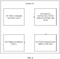
- FIG. 6 is a schematic flowchart of a data processing method 600 according to an embodiment of this application. As shown in FIG. 6 , the method 600 includes the following steps.
- S601 Obtain data from a visual sensor and an inertial sensor IMU, and perform time synchronization on an obtained image and obtained IMU data.
- S602 Extract an environment landmark characteristic vector from visual image information, and perform characteristic matching.
- S603 Establish a nonlinearized constraint equation of the at least one pose vector and/or at least one landmark characteristic vector, where the constraint equation includes a motion equation and an observation equation; the motion equation of an intelligent device is established based on the IMU data in S601 and a motion model; and the observation equation is established based on the landmark characteristic vector extracted in S602, an observation model, and a pose obtained through optimization of a previous frame that are used as prior information.
- S604 Determine a to-be-marginalized state vector, to be specific, determine the to-be-marginalized state vector in the pose vector and the landmark characteristic vector by using a sliding window method or a parallax method.
- S605 Linearize the nonlinearized constraint equation established in S603, to be specific, calculate Jacobian matrices of the motion equation and the observation equation in S603, and linearize the nonlinearized constraint equation in S603 based on the Jacobian matrices to obtain a first linearized constraint equation.
- S606 Rearrange the linearized constraint equation established in S605, and separate the to-be-marginalized state vector from other state vectors in the linearized constraint equation, to be specific, rearrange, based on the to-be-marginalized state vector determined in S604, the first linearized constraint equation established in S605, and separate a to-be-preserved state vector in the first linearized constraint equation from the to-be-marginalized state vector in the first linearized constraint equation.
- S607 Calculate a left null space of a Jacobian matrix of the to-be-marginalized vector, to be specific, calculate the left null space of the to-be-marginalized state vector based on a rearranged first linearized constraint equation obtained in S606.
- S608 Marginalize the state vector, and determine a reduced linearized constraint equation, to be specific, left-multiply the left null space of the to-be-marginalized state vector obtained through calculation in S607, by the rearranged first linearized constraint equation obtained in S606, to obtain a reduced second linearized constraint equation.
- S609 Construct an objective function based on the reduced second linearized constraint equation determined in S608, and calculate a marginalized information matrix.
- S610 Perform graph optimization on the objective function, and construct, based on the information matrix obtained in S609, a prior constraint for next optimization.
- Table 1 shows a calculation time comparison between a Schur complement based marginalization method and a null-space based marginalization method according to an embodiment of this application. It can be learned from Table 1 that running efficiency of the null-space based marginalization method is 4.6 times that of the Schur complement based marginalization method.
- Table 1 Marginalization algorithm Average running time (s) Schur complement based marginalization algorithm 0.0440574 Null-space based marginalization algorithm 0.00953969
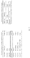
- FIG. 7 shows a calculation step comparison between a null space method according to an embodiment of this application and a Schur complement method.
- calculation complexity of the two methods is compared and analyzed. It is assumed that n landmark characteristics are tracked for m robot poses. Black boxes represent steps that are most time consuming in the two marginalization methods. Usually, n is much greater than m. It can be learned that calculation complexity of the null space method is less than that of the Schur complement method.
- FIG. 8 is a schematic block diagram of a data processing apparatus 700 according to an embodiment of this application. As shown in FIG. 8 , the apparatus 700 includes:
- the marginalization unit 730 is specifically configured to: marginalize the first state vector in the first linearized constraint equation based on a null space of a Jacobian matrix of the first state vector, to obtain the second linearized constraint equation.
- the marginalization unit is specifically configured to:
- the second linearized constraint equation is: U m T z ⁇ ⁇ U m T H u x ⁇ u + U m T n , where x ⁇ u is an error vector of the second state vector, H u is a Jacobian matrix of the second state vector, U m is the null space of the Jacobian matrix of the first state vector, z ⁇ is a residual vector of an observed vector, and n is a white Gaussian noise vector.
- the apparatus 700 further includes: a rearrangement unit, configured to rearrange the first linearized constraint equation based on the first state vector, where the first state vector in the rearranged first linearized constraint equation is separated from the second state vector in the rearranged first linearized constraint equation.
- a rearrangement unit configured to rearrange the first linearized constraint equation based on the first state vector, where the first state vector in the rearranged first linearized constraint equation is separated from the second state vector in the rearranged first linearized constraint equation.
- the rearranged first linearized constraint equation is: z ⁇ ⁇ H u x ⁇ u + H m x ⁇ m + n , where x ⁇ u is the error vector of the second state vector, x ⁇ m is an error vector of the first state vector, H m is the Jacobian matrix of the first state vector, H u is the Jacobian matrix of the second state vector, z ⁇ is the residual vector of the observed vector, and n is the white Gaussian noise vector.
- the determining unit 720 is further configured to: determine an information matrix based on the objective function, where the information matrix is a constraint for next data processing.
- the determining unit is further configured to:
- the determining unit 720 is further configured to: determine an information matrix based on the objective function, where the information matrix is used to optimize and update the second state vector; and construct a new constraint term based on the optimized and updated second state vector, where the constraint term is used to constrain a linearized constraint equation established during next data processing.
- the data processing apparatus 700 may correspond to the SLAM system in the data processing method 200 in the embodiment of this application.
- the data processing apparatus 700 may include modules configured to perform the method performed by the SLAM system in the data processing method 200 in FIG. 2 .
- the modules in the data processing apparatus 700 and the foregoing and other operations and/or functions are respectively used for implementing corresponding procedures in the data processing method 200 in FIG. 2 .
- the obtaining unit 710 is configured to perform step 210 in the method 200;
- the determining unit 720 is configured to perform steps 220, 230, and 250 in the method 200;
- the marginalization unit 730 is configured to perform step 240 in the method 200;
- the optimization unit 740 is configured to perform step 260 in the method 200.
- Specific processes of performing the corresponding steps by the units are already described in detail in the method 200. For brevity, details are not described herein again.
- FIG. 9 is a schematic structural diagram of a data processing apparatus 800 according to an embodiment of this application.
- the data processing apparatus 800 includes a processor 810, a memory 820, and a communications interface 830.
- the memory 820 stores an instruction
- the processor 810 is configured to execute the instruction in the memory 820.
- the processor 510 is configured to perform the method provided in the foregoing method embodiment.
- the processor 810 is further configured to control the communications interface 830 to communicate with the outside.
- the data processing apparatus 800 may correspond to the SLAM system 100 according to the embodiments of this application.
- the data processing apparatus 800 may include modules configured to perform the method performed by the SLAM system 100 in the data processing method 200 in FIG. 2 .
- the modules in the data processing apparatus 800 and the foregoing and other operations and/or functions are respectively used for implementing corresponding procedures in the data processing method 200 in FIG. 2 . Specific processes of performing the corresponding steps by the modules are described in detail in the method 200. For brevity, details are not described herein again.
- An embodiment of this application further provides a computer readable storage medium.
- the computer readable storage medium includes a computer program. When the computer program is run on a computer, the computer is enabled to perform the method provided in the foregoing method embodiment.
- An embodiment of this application further provides a computer program product including an instruction.
- the computer program product When the computer program product is run on a computer, the computer is enabled to perform the method provided in the foregoing method embodiment.
- the processor in the embodiments of this application may be a central processing unit (central processing unit, CPU), or the processor may be another general purpose processor, a digital signal processor (digital signal processor, DSP), an application-specific integrated circuit (application specific integrated circuit, ASIC), a field programmable gate array (field programmable gate array, FPGA) or another programmable logic device, a discrete gate or a transistor logic device, a discrete hardware component, or the like.
- the general purpose processor may be a microprocessor, or the processor may be any conventional processor or the like.
- the memory in the embodiments of this application may be a volatile memory or a nonvolatile memory, or may include both a volatile memory and a nonvolatile memory.
- the nonvolatile memory may be a read-only memory (read-only memory, ROM), a programmable read-only memory (programmable ROM, PROM), an erasable programmable read-only memory (erasable PROM, EPROM), an electrically erasable programmable read-only memory (electrically EPROM, EEPROM), or a flash memory.
- the volatile memory may be a random access memory (random access memory, RAM), used as an external cache.
- random access memory random access memory
- static random access memory static random access memory
- DRAM dynamic random access memory
- SDRAM synchronous dynamic random access memory
- double data rate SDRAM double data rate SDRAM
- DDR SDRAM double data rate SDRAM
- enhanced SDRAM enhanced synchronous dynamic random access memory
- synchlink dynamic random access memory synchlink DRAM, SLDRAM
- direct rambus RAM direct rambus RAM, DR RAM
- the disclosed system, apparatus, and method may be implemented in other manners.
- the described apparatus embodiment is merely an example.
- the unit division is merely logical function division and may be other division in actual implementation.
- a plurality of units or components may be combined or may be integrated into another system, or some features may be ignored or not performed.
- the displayed or discussed mutual couplings or direct couplings or communication connections may be implemented by using some interfaces.
- the indirect couplings or communication connections between the apparatuses or units may be implemented in electrical, mechanical, or other forms.
- the units described as separate parts may or may not be physically separate, and parts displayed as units may or may not be physical units, may be located in one position, or may be distributed on a plurality of network units. Some or all of the units may be selected according to actual requirements, to achieve the objectives of the solutions in the embodiments.
- the functions When the functions are implemented in a form of a software functional unit and sold or used as an independent product, the functions may be stored in a computer readable storage medium. Based on such an understanding, the technical solutions of this application essentially, or the part contributing to the prior art, or some of the technical solutions may be implemented in a form of a software product.
- the computer software product is stored in a storage medium, and includes several instructions for instructing a computer device (which may be a personal computer, a server, a network device, or the like) to perform all or some of the steps of the methods described in the embodiments of this application.
- the foregoing storage medium includes any medium that can store program code, such as a USB flash drive, a removable hard disk, a read-only memory (Read-Only Memory, ROM), a random access memory (Random Access Memory, RAM), a magnetic disk, or an optical disc.
- program code such as a USB flash drive, a removable hard disk, a read-only memory (Read-Only Memory, ROM), a random access memory (Random Access Memory, RAM), a magnetic disk, or an optical disc.
Landscapes
- Engineering & Computer Science (AREA)
- Physics & Mathematics (AREA)
- Radar, Positioning & Navigation (AREA)
- General Physics & Mathematics (AREA)
- Remote Sensing (AREA)
- Automation & Control Theory (AREA)
- Aviation & Aerospace Engineering (AREA)
- Theoretical Computer Science (AREA)
- Computer Vision & Pattern Recognition (AREA)
- Software Systems (AREA)
- Multimedia (AREA)
- Evolutionary Computation (AREA)
- Artificial Intelligence (AREA)
- Mathematical Physics (AREA)
- Data Mining & Analysis (AREA)
- Computing Systems (AREA)
- General Engineering & Computer Science (AREA)
- Electromagnetism (AREA)
- Medical Informatics (AREA)
- Mathematical Optimization (AREA)
- Computational Mathematics (AREA)
- Mathematical Analysis (AREA)
- Algebra (AREA)
- Pure & Applied Mathematics (AREA)
- Probability & Statistics with Applications (AREA)
- Control Of Position, Course, Altitude, Or Attitude Of Moving Bodies (AREA)
- Business, Economics & Management (AREA)
- Health & Medical Sciences (AREA)
- Game Theory and Decision Science (AREA)
Claims (15)
- Procédé de traitement de données, comprenant :l'obtention (210) d'un ensemble de vecteurs d'état d'un dispositif intelligent, dans lequel l'ensemble de vecteurs d'état comprend au moins un vecteur de pose du dispositif intelligent et/ou au moins un vecteur caractéristique de repère d'un environnement dans lequel se trouve le dispositif intelligent, et l'au moins un vecteur de pose et/ou l'au moins un vecteur caractéristique de repère est/sont utilisé(s) pour localiser le dispositif intelligent et cartographier l'environnement dans lequel se trouve l'appareil intelligent ;la détermination (220) d'une première équation de contrainte linéarisée, dans lequel la première équation de contrainte linéarisée est une représentation de contrainte linéarisée de l'au moins un vecteur de pose et/ou de l'au moins un vecteur caractéristique de repère ;la détermination (230) d'un premier vecteur d'état, dans lequel le premier vecteur d'état est un vecteur d'état à marginaliser dans l'ensemble de vecteurs d'état ;la marginalisation (240) du premier vecteur d'état dans la première équation de contrainte linéarisée pour obtenir une seconde équation de contrainte linéarisée, dans lequel la seconde équation de contrainte linéarisée représente une relation de contrainte linéarisée de seconds vecteurs d'état, et le second vecteur d'état est un vecteur d'état autre que le premier vecteur d'état dans l'ensemble de vecteurs d'état ;la détermination (250) d'une fonction objective pour une estimation de probabilité maximale du vecteur d'état sur la base de la seconde équation de contrainte linéarisée ; etl'optimisation (260) de l'au moins un vecteur de pose et/ou de l'au moins un vecteur caractéristique de repère sur la base de la fonction objective, pour émettre une trace du dispositif intelligent et une carte de l'environnement dans lequel se trouve le dispositif intelligent ;le procédé caractérisé par :la détermination d'une matrice d'informations ∑ sur la base de la fonction objective, dans lequel la matrice d'informations est utilisée pour optimiser et mettre à jour le second vecteur d'état ; et la construction d'un nouveau terme de contrainte sur la base du second vecteur d'état optimisé et mis à jour, dans lequel le terme de contrainte est utilisé pour contraindre une équation de contrainte linéarisée établie pendant le traitement de données suivant ; etla réalisation d'une optimisation de graphe sur le second vecteur d'état et la mise à jour du second vecteur d'état en tant que

 où X̃u est un vecteur d'erreur d'un vecteur d'état à conserver, X̂u est une estimation précédente du vecteur d'état à conserver, et
- Procédé selon la revendication 1, dans lequel la marginalisation du premier vecteur d'état dans la première équation de contrainte linéarisée pour obtenir une seconde équation de contrainte linéarisée comprend :la marginalisation du premier vecteur d'état dans la première équation de contrainte linéarisée sur la base d'un espace nul d'une matrice jacobienne du premier vecteur d'état, pour obtenir la seconde équation de contrainte linéarisée.
- Procédé selon la revendication 2, dans lequel la marginalisation du premier vecteur d'état dans la première équation de contrainte linéarisée sur la base d'un espace nul d'une matrice jacobienne du premier vecteur d'état, pour obtenir la seconde équation de contrainte linéarisée, comprend :la détermination de la matrice jacobienne du premier vecteur d'état ;la détermination d'un espace nul gauche de la matrice jacobienne du premier vecteur d'état sur la base de la matrice jacobienne du premier vecteur d'état ; etla multiplication à gauche de l'espace nul gauche de la matrice jacobienne du premier vecteur d'état par la première équation de contrainte linéarisée pour obtenir la seconde équation de contrainte linéarisée.
- Procédé selon la revendication 2 ou 3, dans lequel la seconde équation de contrainte linéarisée est :

X̃u est un vecteur d'erreur du second vecteur d'état, Hu est une matrice jacobienne du second vecteur d'état, Um est l'espace nul de la matrice jacobienne du premier vecteur d'état, Z̃ est un vecteur résiduel d'un vecteur observé, et n est un vecteur de bruit blanc gaussien. - Procédé selon l'une quelconque des revendications 1 à 4, dans lequel, avant la marginalisation du premier vecteur d'état dans la première équation de contrainte linéarisée pour obtenir une seconde équation de contrainte linéarisée, le procédé comprend en outre :la réorganisation de la première équation de contrainte linéarisée sur la base du premier vecteur d'état, dans lequel le premier vecteur d'état dans la première équation de contrainte linéarisée réorganisée est séparé du second vecteur d'état dans la première équation de contrainte linéarisée réorganisée.
- Procédé selon la revendication 5, dans lequel la première équation de contrainte linéarisée réorganisée est :

X̃u est le vecteur d'erreur du second vecteur d'état, X̃m est un vecteur d'erreur du premier vecteur d'état, Hm est la matrice jacobienne du premier vecteur d'état, Hu est la matrice jacobienne du second vecteur d'état, Z̃ est le vecteur résiduel du vecteur observé, et n est le vecteur de bruit blanc gaussien. - Procédé selon l'une quelconque des revendications 1 à 6, dans lequel, avant la détermination d'une première équation de contrainte linéarisée, le procédé comprend en outre :la détermination d'une équation de contrainte non linéarisée de l'au moins un vecteur de pose et/ou de l'au moins un vecteur caractéristique de repère ; etla linéarisation de l'équation de contrainte non linéarisée sur la base d'une matrice jacobienne de l'au moins un vecteur de pose et/ou de l'au moins un vecteur caractéristique de repère, pour obtenir la première équation de contrainte linéarisée.
- Appareil de traitement de données, comprenant :une unité d'obtention (710), configurée pour obtenir un ensemble de vecteurs d'état d'un dispositif intelligent, dans lequel l'ensemble de vecteurs d'état comprend au moins un vecteur de pose du dispositif intelligent et/ou au moins un vecteur caractéristique de repère d'un environnement dans lequel se trouve le dispositif intelligent, et l'au moins un vecteur de pose et/ou l'au moins un vecteur caractéristique de repère est/sont utilisé(s) pour localiser le dispositif intelligent et cartographier l'environnement dans lequel se trouve le dispositif intelligent ;une unité de détermination (720), configurée pour déterminer une première équation de contrainte linéarisée, dans lequel la première équation de contrainte linéarisée est une représentation de contrainte linéarisée de l'au moins un vecteur de pose et/ou de l'au moins un vecteur caractéristique de repère, dans lequell'unité de détermination est en outre configurée pour déterminer un premier vecteur d'état, dans lequel le premier vecteur d'état est un vecteur d'état à marginaliser dans l'ensemble de vecteurs d'état ;une unité de marginalisation (730), configurée pour marginaliser le premier vecteur d'état dans la première équation de contrainte linéarisée pour obtenir une seconde équation de contrainte linéarisée, dans lequel la seconde équation de contrainte linéarisée représente une relation de contrainte linéarisée de seconds vecteurs d'état, et le second vecteur d'état est un vecteur d'état autre que le premier vecteur d'état dans l'ensemble de vecteurs d'état, dans lequell'unité de détermination est en outre configurée pour déterminer une fonction objective pour une estimation de probabilité maximale du vecteur d'état sur la base de la seconde équation de contrainte linéarisée ; etune unité d'optimisation (740), configurée pour optimiser l'au moins un vecteur de pose et/ou l'au moins un vecteur caractéristique de repère sur la base de la fonction objective, pour émettre une trace du dispositif intelligent et une carte de l'environnement dans lequel se trouve le dispositif intelligent ;caractérisé en ce que l'unité de détermination est en outre configurée pour :déterminer une matrice d'informations Σ sur la base de la fonction objective, dans lequel la matrice d'informations est utilisée pour optimiser et mettre à jour le second vecteur d'état ; et la construction d'un nouveau terme de contrainte sur la base du second vecteur d'état optimisé et mis à jour, dans lequel le terme de contrainte est utilisé pour contraindre une équation de contrainte linéarisée établie pendant le traitement de données suivant ; etréaliser une optimisation de graphe sur le second vecteur d'état et la mise à jour du second vecteur d'état en tant que

 où X̃u est un vecteur d'erreur d'un vecteur d'état à conserver, Xu est une estimation précédente du vecteur d'état à conserver, et
- Appareil selon la revendication 8, dans lequel l'unité de marginalisation est spécifiquement configurée pour marginaliser le premier vecteur d'état dans la première équation de contrainte linéarisée sur la base d'un espace nul d'une matrice jacobienne du premier vecteur d'état, pour obtenir la seconde équation de contrainte linéarisée.
- Appareil selon la revendication 9, dans lequel l'unité de marginalisation est configurée spécifiquement pour :déterminer la matrice jacobienne du premier vecteur d'état ;déterminer un espace nul gauche de la matrice jacobienne du premier vecteur d'état sur la base de la matrice jacobienne du premier vecteur d'état ; etmultiplier à gauche l'espace nul gauche de la matrice jacobienne du premier vecteur d'état par la première équation de contrainte linéarisée pour obtenir la seconde équation de contrainte linéarisée.
- Appareil selon la revendication 9 ou 10, dans lequel la seconde équation de contrainte linéarisée est :

X̃u est un vecteur d'erreur du second vecteur d'état, Hu est une matrice jacobienne du second vecteur d'état, Um est l'espace nul de la matrice jacobienne du premier vecteur d'état, Z̃ est un vecteur résiduel d'un vecteur observé, et n est un vecteur de bruit blanc gaussien. - Appareil selon l'une quelconque des revendications 8 à 11, dans lequel l'appareil comprend en outre :
une unité de réorganisation, configurée pour réorganiser la première équation de contrainte linéarisée sur la base du premier vecteur d'état, dans lequel le premier vecteur d'état dans la première équation de contrainte linéarisée réorganisée est séparé du second vecteur d'état dans la première équation de contrainte linéarisée réorganisée. - Appareil selon la revendication 12, dans lequel la première équation de contrainte linéarisée réorganisée est :

X̃u est le vecteur d'erreur du second vecteur d'état, X̃m est un vecteur d'erreur du premier vecteur d'état, Hm est la matrice jacobienne du premier vecteur d'état, Hu est la matrice jacobienne du second vecteur d'état, Z̃ est le vecteur résiduel du vecteur observé, et n est le vecteur de bruit blanc gaussien. - Appareil selon l'une quelconque des revendications 8 à 13, dans lequel l'unité de détermination est en outre configurée pour :déterminer une équation de contrainte non linéarisée de l'au moins un vecteur de pose et/ou de l'au moins un vecteur caractéristique de repère ; etlinéariser l'équation de contrainte non linéarisée sur la base d'une matrice jacobienne de l'au moins un vecteur de pose et/ou de l'au moins un vecteur caractéristique de repère, pour obtenir la première équation de contrainte linéarisée.
- Support de stockage lisible par ordinateur, comprenant un programme informatique, dans lequel, lorsque le programme informatique est exécuté sur un ordinateur, l'ordinateur est capable de mettre en œuvre le procédé de traitement de données selon l'une quelconque des revendications 1 à 7.
Applications Claiming Priority (2)
| Application Number | Priority Date | Filing Date | Title |
|---|---|---|---|
| CN201710868757.6A CN109542093B (zh) | 2017-09-22 | 2017-09-22 | 一种处理数据的方法和装置 |
| PCT/CN2018/106910 WO2019057146A1 (fr) | 2017-09-22 | 2018-09-21 | Procédé et dispositif de traitement de données |
Publications (3)
| Publication Number | Publication Date |
|---|---|
| EP3677978A1 EP3677978A1 (fr) | 2020-07-08 |
| EP3677978A4 EP3677978A4 (fr) | 2020-08-05 |
| EP3677978B1 true EP3677978B1 (fr) | 2022-04-06 |
Family
ID=65811099
Family Applications (1)
| Application Number | Title | Priority Date | Filing Date |
|---|---|---|---|
| EP18857990.8A Not-in-force EP3677978B1 (fr) | 2017-09-22 | 2018-09-21 | Procédé et dispositif de traitement de données |
Country Status (4)
| Country | Link |
|---|---|
| US (1) | US20200219000A1 (fr) |
| EP (1) | EP3677978B1 (fr) |
| CN (1) | CN109542093B (fr) |
| WO (1) | WO2019057146A1 (fr) |
Families Citing this family (4)
| Publication number | Priority date | Publication date | Assignee | Title |
|---|---|---|---|---|
| CN108876854B (zh) * | 2018-04-27 | 2022-03-08 | 腾讯科技(深圳)有限公司 | 相机姿态追踪过程的重定位方法、装置、设备及存储介质 |
| CN111238497B (zh) | 2018-11-29 | 2022-05-06 | 华为技术有限公司 | 一种高精度地图的构建方法及装置 |
| CN111256689B (zh) * | 2020-01-15 | 2022-01-21 | 北京智华机器人科技有限公司 | 一种机器人定位方法、机器人和存储介质 |
| US20250027773A1 (en) * | 2023-07-18 | 2025-01-23 | Qualcomm Incorporated | Inertial navigation aided with multi-interval pose measurements |
Family Cites Families (13)
| Publication number | Priority date | Publication date | Assignee | Title |
|---|---|---|---|---|
| KR100601960B1 (ko) * | 2004-08-05 | 2006-07-14 | 삼성전자주식회사 | 로봇의 위치 추적 및 지도 작성 방법 |
| CN102402225B (zh) * | 2011-11-23 | 2013-09-04 | 中国科学院自动化研究所 | 一种实现移动机器人同时定位与地图构建的方法 |
| CN102706342A (zh) * | 2012-05-31 | 2012-10-03 | 重庆邮电大学 | 一种智能移动机器人的定位与环境建模方法 |
| WO2014130854A1 (fr) * | 2013-02-21 | 2014-08-28 | Regents Of The Univesity Of Minnesota | Étalonnage de paramètre intrinsèque d'un système de navigation inertielle à vision assistée |
| US9607401B2 (en) * | 2013-05-08 | 2017-03-28 | Regents Of The University Of Minnesota | Constrained key frame localization and mapping for vision-aided inertial navigation |
| US20140341465A1 (en) * | 2013-05-16 | 2014-11-20 | The Regents Of The University Of California | Real-time pose estimation system using inertial and feature measurements |
| US10306206B2 (en) * | 2013-07-23 | 2019-05-28 | The Regents Of The University Of California | 3-D motion estimation and online temporal calibration for camera-IMU systems |
| CN103644903B (zh) * | 2013-09-17 | 2016-06-08 | 北京工业大学 | 基于分布式边缘无味粒子滤波的同步定位与地图构建方法 |
| CN103631264A (zh) * | 2013-12-04 | 2014-03-12 | 苏州大学张家港工业技术研究院 | 一种同时定位与地图创建方法及装置 |
| US9658070B2 (en) * | 2014-07-11 | 2017-05-23 | Regents Of The University Of Minnesota | Inverse sliding-window filters for vision-aided inertial navigation systems |
| CN104574387B (zh) * | 2014-12-29 | 2017-11-21 | 张家港江苏科技大学产业技术研究院 | 水下视觉slam系统中的图像处理方法 |
| CN106289181B (zh) * | 2015-05-22 | 2018-12-18 | 北京雷动云合智能技术有限公司 | 一种基于视觉测量的实时slam方法 |
| CN106197428B (zh) * | 2016-07-10 | 2019-03-22 | 北京工业大学 | 一种利用测量信息优化分布式ekf估计过程的slam方法 |
-
2017
- 2017-09-22 CN CN201710868757.6A patent/CN109542093B/zh not_active Expired - Fee Related
-
2018
- 2018-09-21 WO PCT/CN2018/106910 patent/WO2019057146A1/fr not_active Ceased
- 2018-09-21 EP EP18857990.8A patent/EP3677978B1/fr not_active Not-in-force
-
2020
- 2020-03-20 US US16/825,694 patent/US20200219000A1/en not_active Abandoned
Also Published As
| Publication number | Publication date |
|---|---|
| EP3677978A1 (fr) | 2020-07-08 |
| WO2019057146A1 (fr) | 2019-03-28 |
| CN109542093A (zh) | 2019-03-29 |
| CN109542093B (zh) | 2022-06-07 |
| EP3677978A4 (fr) | 2020-08-05 |
| US20200219000A1 (en) | 2020-07-09 |
Similar Documents
| Publication | Publication Date | Title |
|---|---|---|
| US20200219000A1 (en) | Data Processing Method And Apparatus | |
| Wu et al. | A Square Root Inverse Filter for Efficient Vision-aided Inertial Navigation on Mobile Devices. | |
| US9709404B2 (en) | Iterative Kalman Smoother for robust 3D localization for vision-aided inertial navigation | |
| CN111814719B (zh) | 一种基于3d时空图卷积的骨架行为识别方法 | |
| US10748061B2 (en) | Simultaneous localization and mapping with reinforcement learning | |
| CN110118556A (zh) | 一种基于协方差交叉融合slam的机器人定位方法及装置 | |
| US10907971B2 (en) | Square root inverse Schmidt-Kalman filters for vision-aided inertial navigation and mapping | |
| US9317923B2 (en) | Stereo vision apparatus and method | |
| CN104346811B (zh) | 基于视频图像的目标实时追踪方法及其装置 | |
| Ciarfuglia et al. | Evaluation of non-geometric methods for visual odometry | |
| EP2854104A1 (fr) | Localisation et cartographie simultanées semi-denses | |
| CN107369166A (zh) | 一种基于多分辨率神经网络的目标跟踪方法及系统 | |
| CN108073857A (zh) | 动态视觉传感器dvs事件处理的方法及装置 | |
| CN106815594A (zh) | 立体匹配方法及装置 | |
| CN110422175B (zh) | 车辆状态估计方法以及装置、电子设备、存储介质、车辆 | |
| US10019801B2 (en) | Image analysis system and method | |
| Hashemifar et al. | Augmenting visual SLAM with Wi-Fi sensing for indoor applications | |
| CN109685830B (zh) | 目标跟踪方法、装置和设备及计算机存储介质 | |
| CN107657627A (zh) | 基于人脑记忆机制的时空上下文目标跟踪方法 | |
| US10115208B2 (en) | Image characteristic estimation method and device | |
| Guo et al. | Video denoising via online sparse and low-rank matrix decomposition | |
| US12524896B2 (en) | Method and apparatus for estimating depth of image | |
| CN115908481A (zh) | 目标跟踪方法、装置、电子设备和计算机可读存储介质 | |
| Lu et al. | Event-based fast visual-inertial odometry by adaptive slicing of time surface | |
| Tran et al. | A Flexible Multi-camera Visual-inertial Architecture for Robust State Estimation in Challenging Scenarios |
Legal Events
| Date | Code | Title | Description |
|---|---|---|---|
| STAA | Information on the status of an ep patent application or granted ep patent |
Free format text: STATUS: THE INTERNATIONAL PUBLICATION HAS BEEN MADE |
|
| PUAI | Public reference made under article 153(3) epc to a published international application that has entered the european phase |
Free format text: ORIGINAL CODE: 0009012 |
|
| STAA | Information on the status of an ep patent application or granted ep patent |
Free format text: STATUS: REQUEST FOR EXAMINATION WAS MADE |
|
| 17P | Request for examination filed |
Effective date: 20200330 |
|
| AK | Designated contracting states |
Kind code of ref document: A1 Designated state(s): AL AT BE BG CH CY CZ DE DK EE ES FI FR GB GR HR HU IE IS IT LI LT LU LV MC MK MT NL NO PL PT RO RS SE SI SK SM TR |
|
| AX | Request for extension of the european patent |
Extension state: BA ME |
|
| A4 | Supplementary search report drawn up and despatched |
Effective date: 20200707 |
|
| RIC1 | Information provided on ipc code assigned before grant |
Ipc: G06F 17/10 20060101ALI20200701BHEP Ipc: G01C 21/28 20060101ALI20200701BHEP Ipc: G06T 7/246 20170101ALI20200701BHEP Ipc: G06T 7/579 20170101ALI20200701BHEP Ipc: G05D 1/02 20200101AFI20200701BHEP |
|
| DAV | Request for validation of the european patent (deleted) | ||
| DAX | Request for extension of the european patent (deleted) | ||
| STAA | Information on the status of an ep patent application or granted ep patent |
Free format text: STATUS: EXAMINATION IS IN PROGRESS |
|
| 17Q | First examination report despatched |
Effective date: 20210225 |
|
| GRAP | Despatch of communication of intention to grant a patent |
Free format text: ORIGINAL CODE: EPIDOSNIGR1 |
|
| STAA | Information on the status of an ep patent application or granted ep patent |
Free format text: STATUS: GRANT OF PATENT IS INTENDED |
|
| INTG | Intention to grant announced |
Effective date: 20211118 |
|
| INTG | Intention to grant announced |
Effective date: 20211118 |
|
| GRAS | Grant fee paid |
Free format text: ORIGINAL CODE: EPIDOSNIGR3 |
|
| GRAA | (expected) grant |
Free format text: ORIGINAL CODE: 0009210 |
|
| STAA | Information on the status of an ep patent application or granted ep patent |
Free format text: STATUS: THE PATENT HAS BEEN GRANTED |
|
| AK | Designated contracting states |
Kind code of ref document: B1 Designated state(s): AL AT BE BG CH CY CZ DE DK EE ES FI FR GB GR HR HU IE IS IT LI LT LU LV MC MK MT NL NO PL PT RO RS SE SI SK SM TR |
|
| REG | Reference to a national code |
Ref country code: GB Ref legal event code: FG4D |
|
| REG | Reference to a national code |
Ref country code: CH Ref legal event code: EP |
|
| REG | Reference to a national code |
Ref country code: AT Ref legal event code: REF Ref document number: 1481954 Country of ref document: AT Kind code of ref document: T Effective date: 20220415 |
|
| REG | Reference to a national code |
Ref country code: DE Ref legal event code: R096 Ref document number: 602018033585 Country of ref document: DE |
|
| REG | Reference to a national code |
Ref country code: IE Ref legal event code: FG4D |
|
| REG | Reference to a national code |
Ref country code: LT Ref legal event code: MG9D |
|
| REG | Reference to a national code |
Ref country code: NL Ref legal event code: MP Effective date: 20220406 |
|
| REG | Reference to a national code |
Ref country code: AT Ref legal event code: MK05 Ref document number: 1481954 Country of ref document: AT Kind code of ref document: T Effective date: 20220406 |
|
| PG25 | Lapsed in a contracting state [announced via postgrant information from national office to epo] |
Ref country code: NL Free format text: LAPSE BECAUSE OF FAILURE TO SUBMIT A TRANSLATION OF THE DESCRIPTION OR TO PAY THE FEE WITHIN THE PRESCRIBED TIME-LIMIT Effective date: 20220406 |
|
| PG25 | Lapsed in a contracting state [announced via postgrant information from national office to epo] |
Ref country code: SE Free format text: LAPSE BECAUSE OF FAILURE TO SUBMIT A TRANSLATION OF THE DESCRIPTION OR TO PAY THE FEE WITHIN THE PRESCRIBED TIME-LIMIT Effective date: 20220406 Ref country code: PT Free format text: LAPSE BECAUSE OF FAILURE TO SUBMIT A TRANSLATION OF THE DESCRIPTION OR TO PAY THE FEE WITHIN THE PRESCRIBED TIME-LIMIT Effective date: 20220808 Ref country code: NO Free format text: LAPSE BECAUSE OF FAILURE TO SUBMIT A TRANSLATION OF THE DESCRIPTION OR TO PAY THE FEE WITHIN THE PRESCRIBED TIME-LIMIT Effective date: 20220706 Ref country code: LT Free format text: LAPSE BECAUSE OF FAILURE TO SUBMIT A TRANSLATION OF THE DESCRIPTION OR TO PAY THE FEE WITHIN THE PRESCRIBED TIME-LIMIT Effective date: 20220406 Ref country code: HR Free format text: LAPSE BECAUSE OF FAILURE TO SUBMIT A TRANSLATION OF THE DESCRIPTION OR TO PAY THE FEE WITHIN THE PRESCRIBED TIME-LIMIT Effective date: 20220406 Ref country code: GR Free format text: LAPSE BECAUSE OF FAILURE TO SUBMIT A TRANSLATION OF THE DESCRIPTION OR TO PAY THE FEE WITHIN THE PRESCRIBED TIME-LIMIT Effective date: 20220707 Ref country code: FI Free format text: LAPSE BECAUSE OF FAILURE TO SUBMIT A TRANSLATION OF THE DESCRIPTION OR TO PAY THE FEE WITHIN THE PRESCRIBED TIME-LIMIT Effective date: 20220406 Ref country code: ES Free format text: LAPSE BECAUSE OF FAILURE TO SUBMIT A TRANSLATION OF THE DESCRIPTION OR TO PAY THE FEE WITHIN THE PRESCRIBED TIME-LIMIT Effective date: 20220406 Ref country code: BG Free format text: LAPSE BECAUSE OF FAILURE TO SUBMIT A TRANSLATION OF THE DESCRIPTION OR TO PAY THE FEE WITHIN THE PRESCRIBED TIME-LIMIT Effective date: 20220706 Ref country code: AT Free format text: LAPSE BECAUSE OF FAILURE TO SUBMIT A TRANSLATION OF THE DESCRIPTION OR TO PAY THE FEE WITHIN THE PRESCRIBED TIME-LIMIT Effective date: 20220406 |
|
| PG25 | Lapsed in a contracting state [announced via postgrant information from national office to epo] |
Ref country code: RS Free format text: LAPSE BECAUSE OF FAILURE TO SUBMIT A TRANSLATION OF THE DESCRIPTION OR TO PAY THE FEE WITHIN THE PRESCRIBED TIME-LIMIT Effective date: 20220406 Ref country code: PL Free format text: LAPSE BECAUSE OF FAILURE TO SUBMIT A TRANSLATION OF THE DESCRIPTION OR TO PAY THE FEE WITHIN THE PRESCRIBED TIME-LIMIT Effective date: 20220406 Ref country code: LV Free format text: LAPSE BECAUSE OF FAILURE TO SUBMIT A TRANSLATION OF THE DESCRIPTION OR TO PAY THE FEE WITHIN THE PRESCRIBED TIME-LIMIT Effective date: 20220406 Ref country code: IS Free format text: LAPSE BECAUSE OF FAILURE TO SUBMIT A TRANSLATION OF THE DESCRIPTION OR TO PAY THE FEE WITHIN THE PRESCRIBED TIME-LIMIT Effective date: 20220806 |
|
| REG | Reference to a national code |
Ref country code: DE Ref legal event code: R097 Ref document number: 602018033585 Country of ref document: DE |
|
| PG25 | Lapsed in a contracting state [announced via postgrant information from national office to epo] |
Ref country code: SM Free format text: LAPSE BECAUSE OF FAILURE TO SUBMIT A TRANSLATION OF THE DESCRIPTION OR TO PAY THE FEE WITHIN THE PRESCRIBED TIME-LIMIT Effective date: 20220406 Ref country code: SK Free format text: LAPSE BECAUSE OF FAILURE TO SUBMIT A TRANSLATION OF THE DESCRIPTION OR TO PAY THE FEE WITHIN THE PRESCRIBED TIME-LIMIT Effective date: 20220406 Ref country code: RO Free format text: LAPSE BECAUSE OF FAILURE TO SUBMIT A TRANSLATION OF THE DESCRIPTION OR TO PAY THE FEE WITHIN THE PRESCRIBED TIME-LIMIT Effective date: 20220406 Ref country code: EE Free format text: LAPSE BECAUSE OF FAILURE TO SUBMIT A TRANSLATION OF THE DESCRIPTION OR TO PAY THE FEE WITHIN THE PRESCRIBED TIME-LIMIT Effective date: 20220406 Ref country code: DK Free format text: LAPSE BECAUSE OF FAILURE TO SUBMIT A TRANSLATION OF THE DESCRIPTION OR TO PAY THE FEE WITHIN THE PRESCRIBED TIME-LIMIT Effective date: 20220406 Ref country code: CZ Free format text: LAPSE BECAUSE OF FAILURE TO SUBMIT A TRANSLATION OF THE DESCRIPTION OR TO PAY THE FEE WITHIN THE PRESCRIBED TIME-LIMIT Effective date: 20220406 |
|
| PLBE | No opposition filed within time limit |
Free format text: ORIGINAL CODE: 0009261 |
|
| STAA | Information on the status of an ep patent application or granted ep patent |
Free format text: STATUS: NO OPPOSITION FILED WITHIN TIME LIMIT |
|
| 26N | No opposition filed |
Effective date: 20230110 |
|
| PG25 | Lapsed in a contracting state [announced via postgrant information from national office to epo] |
Ref country code: AL Free format text: LAPSE BECAUSE OF FAILURE TO SUBMIT A TRANSLATION OF THE DESCRIPTION OR TO PAY THE FEE WITHIN THE PRESCRIBED TIME-LIMIT Effective date: 20220406 |
|
| PG25 | Lapsed in a contracting state [announced via postgrant information from national office to epo] |
Ref country code: MC Free format text: LAPSE BECAUSE OF FAILURE TO SUBMIT A TRANSLATION OF THE DESCRIPTION OR TO PAY THE FEE WITHIN THE PRESCRIBED TIME-LIMIT Effective date: 20220406 |
|
| REG | Reference to a national code |
Ref country code: CH Ref legal event code: PL |
|
| REG | Reference to a national code |
Ref country code: BE Ref legal event code: MM Effective date: 20220930 |
|
| PG25 | Lapsed in a contracting state [announced via postgrant information from national office to epo] |
Ref country code: SI Free format text: LAPSE BECAUSE OF FAILURE TO SUBMIT A TRANSLATION OF THE DESCRIPTION OR TO PAY THE FEE WITHIN THE PRESCRIBED TIME-LIMIT Effective date: 20220406 |
|
| P01 | Opt-out of the competence of the unified patent court (upc) registered |
Effective date: 20230524 |
|
| PG25 | Lapsed in a contracting state [announced via postgrant information from national office to epo] |
Ref country code: LU Free format text: LAPSE BECAUSE OF NON-PAYMENT OF DUE FEES Effective date: 20220921 |
|
| PG25 | Lapsed in a contracting state [announced via postgrant information from national office to epo] |
Ref country code: LI Free format text: LAPSE BECAUSE OF NON-PAYMENT OF DUE FEES Effective date: 20220930 Ref country code: IE Free format text: LAPSE BECAUSE OF NON-PAYMENT OF DUE FEES Effective date: 20220921 Ref country code: CH Free format text: LAPSE BECAUSE OF NON-PAYMENT OF DUE FEES Effective date: 20220930 |
|
| PG25 | Lapsed in a contracting state [announced via postgrant information from national office to epo] |
Ref country code: BE Free format text: LAPSE BECAUSE OF NON-PAYMENT OF DUE FEES Effective date: 20220930 |
|
| PGFP | Annual fee paid to national office [announced via postgrant information from national office to epo] |
Ref country code: GB Payment date: 20230803 Year of fee payment: 6 |
|
| REG | Reference to a national code |
Ref country code: DE Ref legal event code: R079 Ref document number: 602018033585 Country of ref document: DE Free format text: PREVIOUS MAIN CLASS: G05D0001020000 Ipc: G05D0001430000 |
|
| PGFP | Annual fee paid to national office [announced via postgrant information from national office to epo] |
Ref country code: FR Payment date: 20230808 Year of fee payment: 6 Ref country code: DE Payment date: 20230802 Year of fee payment: 6 |
|
| PG25 | Lapsed in a contracting state [announced via postgrant information from national office to epo] |
Ref country code: IT Free format text: LAPSE BECAUSE OF FAILURE TO SUBMIT A TRANSLATION OF THE DESCRIPTION OR TO PAY THE FEE WITHIN THE PRESCRIBED TIME-LIMIT Effective date: 20220406 |
|
| PG25 | Lapsed in a contracting state [announced via postgrant information from national office to epo] |
Ref country code: CY Free format text: LAPSE BECAUSE OF FAILURE TO SUBMIT A TRANSLATION OF THE DESCRIPTION OR TO PAY THE FEE WITHIN THE PRESCRIBED TIME-LIMIT Effective date: 20220406 |
|
| PG25 | Lapsed in a contracting state [announced via postgrant information from national office to epo] |
Ref country code: MK Free format text: LAPSE BECAUSE OF FAILURE TO SUBMIT A TRANSLATION OF THE DESCRIPTION OR TO PAY THE FEE WITHIN THE PRESCRIBED TIME-LIMIT Effective date: 20220406 Ref country code: HU Free format text: LAPSE BECAUSE OF FAILURE TO SUBMIT A TRANSLATION OF THE DESCRIPTION OR TO PAY THE FEE WITHIN THE PRESCRIBED TIME-LIMIT; INVALID AB INITIO Effective date: 20180921 |
|
| PG25 | Lapsed in a contracting state [announced via postgrant information from national office to epo] |
Ref country code: TR Free format text: LAPSE BECAUSE OF FAILURE TO SUBMIT A TRANSLATION OF THE DESCRIPTION OR TO PAY THE FEE WITHIN THE PRESCRIBED TIME-LIMIT Effective date: 20220406 |
|
| PG25 | Lapsed in a contracting state [announced via postgrant information from national office to epo] |
Ref country code: MT Free format text: LAPSE BECAUSE OF FAILURE TO SUBMIT A TRANSLATION OF THE DESCRIPTION OR TO PAY THE FEE WITHIN THE PRESCRIBED TIME-LIMIT Effective date: 20220406 |
|
| PG25 | Lapsed in a contracting state [announced via postgrant information from national office to epo] |
Ref country code: BG Free format text: LAPSE BECAUSE OF FAILURE TO SUBMIT A TRANSLATION OF THE DESCRIPTION OR TO PAY THE FEE WITHIN THE PRESCRIBED TIME-LIMIT Effective date: 20220406 |
|
| PG25 | Lapsed in a contracting state [announced via postgrant information from national office to epo] |
Ref country code: BG Free format text: LAPSE BECAUSE OF FAILURE TO SUBMIT A TRANSLATION OF THE DESCRIPTION OR TO PAY THE FEE WITHIN THE PRESCRIBED TIME-LIMIT Effective date: 20220406 |
|
| REG | Reference to a national code |
Ref country code: DE Ref legal event code: R119 Ref document number: 602018033585 Country of ref document: DE |
|
| GBPC | Gb: european patent ceased through non-payment of renewal fee |
Effective date: 20240921 |
|
| PG25 | Lapsed in a contracting state [announced via postgrant information from national office to epo] |
Ref country code: DE Free format text: LAPSE BECAUSE OF NON-PAYMENT OF DUE FEES Effective date: 20250401 |
|
| PG25 | Lapsed in a contracting state [announced via postgrant information from national office to epo] |
Ref country code: GB Free format text: LAPSE BECAUSE OF NON-PAYMENT OF DUE FEES Effective date: 20240921 |
|
| PG25 | Lapsed in a contracting state [announced via postgrant information from national office to epo] |
Ref country code: FR Free format text: LAPSE BECAUSE OF NON-PAYMENT OF DUE FEES Effective date: 20240930 |