EP3695378B1 - Suivi en imagerie ultrasonore - Google Patents
Suivi en imagerie ultrasonore Download PDFInfo
- Publication number
- EP3695378B1 EP3695378B1 EP18788835.9A EP18788835A EP3695378B1 EP 3695378 B1 EP3695378 B1 EP 3695378B1 EP 18788835 A EP18788835 A EP 18788835A EP 3695378 B1 EP3695378 B1 EP 3695378B1
- Authority
- EP
- European Patent Office
- Prior art keywords
- contrast
- frames
- contrast element
- element signal
- optionally
- Prior art date
- Legal status (The legal status is an assumption and is not a legal conclusion. Google has not performed a legal analysis and makes no representation as to the accuracy of the status listed.)
- Active
Links
Images



Classifications
-
- G—PHYSICS
- G06—COMPUTING OR CALCULATING; COUNTING
- G06T—IMAGE DATA PROCESSING OR GENERATION, IN GENERAL
- G06T7/00—Image analysis
- G06T7/20—Analysis of motion
- G06T7/246—Analysis of motion using feature-based methods, e.g. the tracking of corners or segments
- G06T7/248—Analysis of motion using feature-based methods, e.g. the tracking of corners or segments involving reference images or patches
-
- A—HUMAN NECESSITIES
- A61—MEDICAL OR VETERINARY SCIENCE; HYGIENE
- A61B—DIAGNOSIS; SURGERY; IDENTIFICATION
- A61B8/00—Diagnosis using ultrasonic, sonic or infrasonic waves
- A61B8/08—Clinical applications
- A61B8/0891—Clinical applications for diagnosis of blood vessels
-
- A—HUMAN NECESSITIES
- A61—MEDICAL OR VETERINARY SCIENCE; HYGIENE
- A61B—DIAGNOSIS; SURGERY; IDENTIFICATION
- A61B8/00—Diagnosis using ultrasonic, sonic or infrasonic waves
- A61B8/46—Ultrasonic, sonic or infrasonic diagnostic devices with special arrangements for interfacing with the operator or the patient
- A61B8/461—Displaying means of special interest
- A61B8/466—Displaying means of special interest adapted to display 3D data
-
- A—HUMAN NECESSITIES
- A61—MEDICAL OR VETERINARY SCIENCE; HYGIENE
- A61B—DIAGNOSIS; SURGERY; IDENTIFICATION
- A61B8/00—Diagnosis using ultrasonic, sonic or infrasonic waves
- A61B8/48—Diagnostic techniques
- A61B8/481—Diagnostic techniques involving the use of contrast agents, e.g. microbubbles introduced into the bloodstream
-
- A—HUMAN NECESSITIES
- A61—MEDICAL OR VETERINARY SCIENCE; HYGIENE
- A61B—DIAGNOSIS; SURGERY; IDENTIFICATION
- A61B8/00—Diagnosis using ultrasonic, sonic or infrasonic waves
- A61B8/48—Diagnostic techniques
- A61B8/483—Diagnostic techniques involving the acquisition of a 3D volume of data
-
- A—HUMAN NECESSITIES
- A61—MEDICAL OR VETERINARY SCIENCE; HYGIENE
- A61B—DIAGNOSIS; SURGERY; IDENTIFICATION
- A61B8/00—Diagnosis using ultrasonic, sonic or infrasonic waves
- A61B8/52—Devices using data or image processing specially adapted for diagnosis using ultrasonic, sonic or infrasonic waves
- A61B8/5207—Devices using data or image processing specially adapted for diagnosis using ultrasonic, sonic or infrasonic waves involving processing of raw data to produce diagnostic data, e.g. for generating an image
-
- A—HUMAN NECESSITIES
- A61—MEDICAL OR VETERINARY SCIENCE; HYGIENE
- A61B—DIAGNOSIS; SURGERY; IDENTIFICATION
- A61B8/00—Diagnosis using ultrasonic, sonic or infrasonic waves
- A61B8/52—Devices using data or image processing specially adapted for diagnosis using ultrasonic, sonic or infrasonic waves
- A61B8/5215—Devices using data or image processing specially adapted for diagnosis using ultrasonic, sonic or infrasonic waves involving processing of medical diagnostic data
- A61B8/5223—Devices using data or image processing specially adapted for diagnosis using ultrasonic, sonic or infrasonic waves involving processing of medical diagnostic data for extracting a diagnostic or physiological parameter from medical diagnostic data
-
- A—HUMAN NECESSITIES
- A61—MEDICAL OR VETERINARY SCIENCE; HYGIENE
- A61B—DIAGNOSIS; SURGERY; IDENTIFICATION
- A61B8/00—Diagnosis using ultrasonic, sonic or infrasonic waves
- A61B8/52—Devices using data or image processing specially adapted for diagnosis using ultrasonic, sonic or infrasonic waves
- A61B8/5215—Devices using data or image processing specially adapted for diagnosis using ultrasonic, sonic or infrasonic waves involving processing of medical diagnostic data
- A61B8/5238—Devices using data or image processing specially adapted for diagnosis using ultrasonic, sonic or infrasonic waves involving processing of medical diagnostic data for combining image data of patient, e.g. merging several images from different acquisition modes into one image
- A61B8/5246—Devices using data or image processing specially adapted for diagnosis using ultrasonic, sonic or infrasonic waves involving processing of medical diagnostic data for combining image data of patient, e.g. merging several images from different acquisition modes into one image combining images from the same or different imaging techniques, e.g. color Doppler and B-mode
-
- G—PHYSICS
- G06—COMPUTING OR CALCULATING; COUNTING
- G06T—IMAGE DATA PROCESSING OR GENERATION, IN GENERAL
- G06T7/00—Image analysis
- G06T7/0002—Inspection of images, e.g. flaw detection
- G06T7/0012—Biomedical image inspection
- G06T7/0014—Biomedical image inspection using an image reference approach
-
- G—PHYSICS
- G06—COMPUTING OR CALCULATING; COUNTING
- G06T—IMAGE DATA PROCESSING OR GENERATION, IN GENERAL
- G06T7/00—Image analysis
- G06T7/10—Segmentation; Edge detection
-
- G—PHYSICS
- G06—COMPUTING OR CALCULATING; COUNTING
- G06T—IMAGE DATA PROCESSING OR GENERATION, IN GENERAL
- G06T7/00—Image analysis
- G06T7/20—Analysis of motion
-
- G—PHYSICS
- G06—COMPUTING OR CALCULATING; COUNTING
- G06T—IMAGE DATA PROCESSING OR GENERATION, IN GENERAL
- G06T7/00—Image analysis
- G06T7/70—Determining position or orientation of objects or cameras
- G06T7/73—Determining position or orientation of objects or cameras using feature-based methods
-
- G—PHYSICS
- G16—INFORMATION AND COMMUNICATION TECHNOLOGY [ICT] SPECIALLY ADAPTED FOR SPECIFIC APPLICATION FIELDS
- G16H—HEALTHCARE INFORMATICS, i.e. INFORMATION AND COMMUNICATION TECHNOLOGY [ICT] SPECIALLY ADAPTED FOR THE HANDLING OR PROCESSING OF MEDICAL OR HEALTHCARE DATA
- G16H30/00—ICT specially adapted for the handling or processing of medical images
- G16H30/40—ICT specially adapted for the handling or processing of medical images for processing medical images, e.g. editing
-
- G—PHYSICS
- G16—INFORMATION AND COMMUNICATION TECHNOLOGY [ICT] SPECIALLY ADAPTED FOR SPECIFIC APPLICATION FIELDS
- G16H—HEALTHCARE INFORMATICS, i.e. INFORMATION AND COMMUNICATION TECHNOLOGY [ICT] SPECIALLY ADAPTED FOR THE HANDLING OR PROCESSING OF MEDICAL OR HEALTHCARE DATA
- G16H50/00—ICT specially adapted for medical diagnosis, medical simulation or medical data mining; ICT specially adapted for detecting, monitoring or modelling epidemics or pandemics
- G16H50/30—ICT specially adapted for medical diagnosis, medical simulation or medical data mining; ICT specially adapted for detecting, monitoring or modelling epidemics or pandemics for calculating health indices; for individual health risk assessment
-
- G—PHYSICS
- G16—INFORMATION AND COMMUNICATION TECHNOLOGY [ICT] SPECIALLY ADAPTED FOR SPECIFIC APPLICATION FIELDS
- G16H—HEALTHCARE INFORMATICS, i.e. INFORMATION AND COMMUNICATION TECHNOLOGY [ICT] SPECIALLY ADAPTED FOR THE HANDLING OR PROCESSING OF MEDICAL OR HEALTHCARE DATA
- G16H50/00—ICT specially adapted for medical diagnosis, medical simulation or medical data mining; ICT specially adapted for detecting, monitoring or modelling epidemics or pandemics
- G16H50/50—ICT specially adapted for medical diagnosis, medical simulation or medical data mining; ICT specially adapted for detecting, monitoring or modelling epidemics or pandemics for simulation or modelling of medical disorders
-
- A—HUMAN NECESSITIES
- A61—MEDICAL OR VETERINARY SCIENCE; HYGIENE
- A61B—DIAGNOSIS; SURGERY; IDENTIFICATION
- A61B8/00—Diagnosis using ultrasonic, sonic or infrasonic waves
- A61B8/06—Measuring blood flow
-
- G—PHYSICS
- G06—COMPUTING OR CALCULATING; COUNTING
- G06T—IMAGE DATA PROCESSING OR GENERATION, IN GENERAL
- G06T2207/00—Indexing scheme for image analysis or image enhancement
- G06T2207/10—Image acquisition modality
- G06T2207/10016—Video; Image sequence
-
- G—PHYSICS
- G06—COMPUTING OR CALCULATING; COUNTING
- G06T—IMAGE DATA PROCESSING OR GENERATION, IN GENERAL
- G06T2207/00—Indexing scheme for image analysis or image enhancement
- G06T2207/10—Image acquisition modality
- G06T2207/10132—Ultrasound image
-
- G—PHYSICS
- G06—COMPUTING OR CALCULATING; COUNTING
- G06T—IMAGE DATA PROCESSING OR GENERATION, IN GENERAL
- G06T2207/00—Indexing scheme for image analysis or image enhancement
- G06T2207/30—Subject of image; Context of image processing
- G06T2207/30004—Biomedical image processing
- G06T2207/30101—Blood vessel; Artery; Vein; Vascular
Definitions
- the spatial resolution of conventional ultrasound imaging systems may be determined by the diffraction limit.
- the interference of emitted wave-fronts may reduce the focussing capability of an aperture.
- Objects that are smaller than the diffraction limit may be resolved, but due to the diffraction of the beam and the duration of transmitted pulses they may appear to have a size of the Point Spread Function (PSF).
- the PSF may be comparable to the wavelength of the applied sound wave.
- Contrast Enhanced Ultrasound is a known method involving injecting a suitable contrast medium, for example microbubbles, into a vascular system of a subject, in order to provide video data of their kinetics in the vascular bed.
- a suitable contrast medium for example microbubbles
- the usage of microbubbles as ultrasound contrast agents is well known, see for example: V. Sboros, "Response of contrast agents to ultrasound," Adv Drug Deliv Rev, vol. 60, pp. 1117-36, Jun 30 2008 and V. Sboros and M. X. Tang.
- the contrast of the microbubbles can be enhanced using signal processing, for example, by phase or amplitude modulated pulse sequences, to achieve tissue echo cancellation. Microbubble contrast-only images may be produced.
- CEUS During CEUS, data capture typically lasts for an extended period of time. The data may be processed to macroscopically assess the blood flow and/or a volume in large regions of interest in the image that normally encompass large parts of organs.
- CEUS is limited to qualitative or relative measurements of flow and volume. Furthermore, the resolution provided by CEUS is limited to within the diffraction limit.
- the structure of the vascular bed can be probed in a resolution that is beyond the diffraction limit at a near microscopic level.
- Point source localisation shows promising results using CEUS and the first in vivo images show at least a 5-fold resolution improvement at diagnostic frequencies (6.5MHz), as shown in O. M. Viessmann, R. J. Eckersley, K. Christensen-Jeffries, M. X. Tang, and C. Dunsby, "Acoustic super-resolution with ultrasound and microbubbles," Phys Med Biol, vol. 58, pp. 6447-58, Sep 21 2013 .
- a super-resolution vascular imaging technique using ultrafast ultrasound in the rat cortex is discussed in: C. Errico, J. Pierre, S. Pezet, Y. Desailly, Z. Lenkei, O. Couture, et al., "Ultrafast ultrasound localization microscopy for deep super-resolution vascular imaging," Nature, vol. 527, pp. 499-502, Nov 26 2015 .
- the technique exploits microbubble spatial overlap in successive frames with autocorrelation algorithms to extract quantitative measures of velocity.
- the frame rates used require plane wave transmission with limited penetration depth meaning that clinical applications are likely to be limited to small regions of interest.
- the use of plane wave imaging may also be limited in quantifying the vascular dynamics. This is because the microbubble detection efficiency will vary across the image as a result of the large variation of the acoustic field.
- Another MCMC data association algorithm is implemented in D. Ackermann and G. Schmitz, "Detection and Tracking of Multiple Microbubbles in Ultrasound B-Mode Images," IEEE Trans. Ultrason., Ferroelec., Freq. Contr, vol. vol. 63, no. 1, pp. pp. 72-82,, Jan. 2016 .
- This method is based on linking multiple instances of single particles based on the location of single microbubbles.
- Each of the frames may represent a view of the region of the subject, and for at least some of the multiple contrast element signal portions, the multiple contrast element signal portion may be representative of separated contrast elements that appear to overlap according to said view.
- Each of the multiple contrast element signal portions may be representative of separated contrast elements that appear in front of or behind each other according to said view.
- the method may further comprise classifying for each of the frames the one or more identified signal portions as either being a single contrast element signal portion or a multiple contrast element signal portion.
- the linking model may be configured to determine whether there has been a contrast element merging event and/or a contrast element splitting event and/or a contrast element disappearance event and/or a contrast element movement event between at least one of the frames and at least one other of the frames.
- the linking model may be operable to link at least one single contrast element signal portion in at least one of the frames to a multiple contrast element signal portion in a subsequent at least one other of the frames.
- the linking model may be operable to link a multiple contrast element signal portion in at least one of the frames to at least one single contrast element signal portion in a subsequent at least one other of the frames.
- the linking model may be operable to link a multiple contrast element signal portion representing a first number of contrast elements in at least one of the frames to a multiple contrast element signal portion representing a second, different number of contrast elements in at least one of the frames.
- the assigning of position data to each of the single contrast element signal portions and each of the multiple contrast element signal portions may comprise assigning a respective single position value to each of the single contrast element signal portions and each of the multiple contrast element signal portions.
- the ultrasound imaging data may represent intensity as a function of position with a first position resolution
- the assigning of position data to a contrast element signal portion may be based on the variation of intensity with position for said contrast element signal portion
- the assigned position data may have a second position resolution that is greater than said first position resolution
- the second position resolution may be at least 4 times the first position resolution optionally at least 9 times the first position resolution.
- the assigning of position data to a contrast element signal portion may comprise fitting a mathematical function to determine a position using at least one of: intensity, shape and size of signal portion.
- the method may further comprise assigning velocity or speed data to the one or more signal portions.
- the identifying may comprise performing a segmentation process to determine the presence of single or multiple microbubbles.
- the segmentation process may comprise applying at least one of a fitting, filtering and/ or transform process, optionally a watershed transform process.
- the segmentation process may be performed on a modified version of the data of each frame, optionally a smoothed and/or filtered and/or inverted version of the data of each frame.
- the identifying of one or more portions of the ultrasound imaging data as being representative of a contrast element or plurality of contrast elements may comprise identifying candidate contrast element signal portions and optionally performing a thresholding or filtering process to exclude at least some of said candidate contrast element signal portions.
- the identifying of one or more portions of the ultrasound imaging data as being representative of a contrast element or plurality of contrast elements may be at least partially unconstrained by the number of portions of ultrasound imaging data identified as being representative of a contrast element or plurality of contrast elements for at least one other of the frames, optionally such that the number of contrast elements identified can be different for different ones of frames, optionally such that the number of contrast elements identified for at least one of the frames is substantially independent of a number of contrast elements identified for at least one other of the frames.
- the method may further comprise identifying, for at least some of the frames, each of more than 10, optionally more than 100, optionally more than 500, optionally more than 1,000 portions of the ultrasound imaging data per frame as being representative of respective single or multiple contrast elements.
- the sequence of frames may represent a measurement period having a duration in between at least one of: 1 second and 10 seconds; 10 seconds and 30 seconds; 30 seconds and 1 minute; less than 5 minutes.
- the sequence of frames may comprise a frame rate in the range of 10 frames per second to 50 frames per second, optionally higher than 50 frames per second.
- At least some of the contrast elements may be present in vessels in the human or animal subject.
- the method may comprise using said tracking said movement of contrast elements through said region to track the paths of at least some of said vessels.
- At least some of the contrast elements may be present outside vessels in the human or animal subject, and the method may comprise tracking said movement of contrast elements outside the vessels.
- the method may further comprise using said tracking to provide a measure of pulsatile motion or other motion of the subject.
- the vessels may comprise blood vessels and the method may comprise using said tracking of said movement of contrast elements through said region to track passage of blood into, out of, or through at least one anatomical feature of interest, optionally the anatomical feature comprises at least one tumour or organ.
- the vessels may have a range of sizes
- the method may comprise, for at least some of the frames, identifying contrast elements in vessels that have a range of different sizes, optionally at least some of said vessels of said range having cross-sections and/or flow rates that are at least 2 times, optionally 5 times, optionally 10 times, optionally 100 times larger than at least other of said vessels.
- the sequence of frames may each comprise ultrasound imaging data obtained by ultrasound measurements on a living human or animal subject.
- the linking of single or multiple contrast element signal portions thereby to track movement of contrast elements may comprise forming track segments between consecutive frames using the position data for the single and multiple contrast element signal portions and joining the formed track segments to produce a plurality of contrast element tracks.
- the joining of the track segments may comprise at least one of gap closing, merging and splitting, optionally based on at least one of size, distance, signal intensity and motion direction.
- the method may further comprise introducing the contrast elements into the subject, optionally using at least one of bolus or continuous infusion.
- an image processing system comprising a processing resource configured to: receive a sequence of frames each comprising ultrasound or other medical imaging data representing an anatomical region of a human or animal subject at a respective different time; for each frame, identify one or more portions of the ultrasound or other medical imaging data wherein the identified portions comprise both at least one single contrast element signal portion and at least one multiple contrast element signal portion, each single contrast element signal portion being representative of a contrast element and each multiple contrast element signal portion being representative of a plurality of contrast elements; assign respective position data to each of the single contrast element signal portions and assign respective position data to each of the multiple contrast element signal portions; and use a linking model that uses at least said assigned position data to link single or multiple contrast element signal portions represented in at least one of the frames to single or multiple contrast element signal portions represented in at least one other of the frames thereby to track movement of contrast elements through said region of the subject.
- An imaging system comprising: an ultrasound scanner, or other scanner, configured to perform a scan of a human or animal subject to obtained a sequence of frames; and an image processing system as claimed or described herein configured to receive and process the sequence of frames to track movement of contrast elements through a region of the subject.
- a computer program product comprising computer-readable instructions that are executable to perform a method as claimed or described herein.
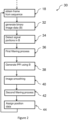
- Figure 1 shows a flowchart outlining the main steps of an ultrasound imaging method 10.
- the method 10 is directed to processing medical images of an anatomical region of a human or animal subject, following administration of a suitable contrast medium, for example microbubbles, to the subject.
- the medical images are captured over a period of time to allow the movement of the contrast medium through the anatomical region to be analysed.
- the period of time may have a duration of, for example, seconds to minutes. Signals from microbubbles can be sensed using ultrasound methods.
- the contrast elements may be microbubbles or any suitable contrast media, for example, nanoparticles or contrast agent particles (CAP).
- suitable imaging techniques other than ultrasound may be used, for example, CT scans, magnetic resonance (MR) scans, positron emission tomography (PET) scans.
- a first step 12 of method 10 is obtaining a plurality of frames of a frame sequence, that have been acquired using ultrasound imaging. Each frame represents ultrasound image data.
- Method 10 is described using ultrasound image data representing microbubbles, however, other image data may be obtained using other medical imaging techniques, for example, computerised tomography (CT) scans, magnetic resonance (MR), positron emission tomography (PET) and suitable contrast media may be used.
- CT computerised tomography
- MR magnetic resonance
- PET positron emission tomography
- suitable contrast media may be used.
- the frame sequence and image data are representative of the anatomical region of the human or animal subject, captured over a period of time.
- Each frame therefore comprises ultrasound imaging data that represents the anatomical region at a different time.
- the sequence of frames is captured by performing ultrasound measurements on the living human or animal subject.
- the ultrasound measurements represent the presence of microbubbles administered to the subject.
- the data capture may take place at the same time as the frame processing, or data capture and frame processing may take place at different times.
- the sequence of frames may be stored and later obtained for the frame processing.
- An example ultrasound apparatus for capturing a sequence of frames is illustrated in Figure 1 .
- Microbubbles are contrast enhancing agents that act as targets in ultrasound methods.
- a microbubble may comprise a bubble that, on average, has a size of less than 1 one millimetre in diameter but larger than one micrometre.
- a solution of microbubbles will contain microbubbles that vary in size and shape.
- Microbubbles may have a diameter of 1 to 10 micrometres.
- microbubbles are introducing into the subject using either bolus or continuous infusion.
- the microbubbles are infused into the subject at a rate that enables a sparse distribution of particles in the frames.
- a suitable infusion rate may be determined experimentally or pre-determined. Infusion rate is determined and dependent on a number of factors, for example, human physiology, microbubble suspension density, imaging system.
- the suspension density has to be such that the microbubbles can be separated, for example, as shown in Figure 3(a) . In some embodiments, any suitable suspension density is used.
- the region to be imaged is part of the vascular bed of the subject.
- the microbubbles travel through the vascular bed and by imaging the microbubbles the structure of the vascular bed is revealed.
- a typical vessel has a size of millimetres to a few microns.
- the vessels comprise blood vessels and the method uses tracking of said movement of microbubbles through said region to track passage of blood into, out of, or through the anatomical feature of interest.
- the anatomical feature may be a tumour or organ.
- Each frame is composed of pixels.
- the pixel size is typically 100 micrometres. In some embodiments, the pixel size is in the range of about 10 to about 1000 micrometres. The pixel size is therefore larger than the microbubble to be imaged. However, the signal from the microbubble may have the size of several pixels in the image. This is because it will occupy the size of the point spread function (PSF).
- PSF point spread function
- the point spread function is the response of the imaging system to the imaged microbubble.
- Each frame represents a view of the region of the subject.
- microbubbles may appear to overlap in the obtained ultrasound image.
- the position resolution can be selected to be greater than the pixel resolution.
- the sequence of frames may be characterised using the period of time which they represent. Any time period suitable to gather the data to image the region of interest can be used.
- the sequence of frames may be characterised using a frame rate.
- the frame rate may take any suitable value.
- a second step 14 is directed to pre-processing the obtained sequence of frames.
- the second step 14 has three main components.
- a first component is an image registration process. This process is performed on each frame of the sequence of frames.
- the image registration process is a rigid image registration. The image registration process acts to generate a substantially motionless sequence of frames or video loop.
- the registration process acts to substantially remove image deformation or image artefacts from externally induced motion, for example, operator probe movement.
- an alternative image registration process is performed, for example, a non-rigid image registration.
- the image registration process may be optional.
- a second component of the pre-processing step is a filtering process performed on each frame of the sequence of frames.
- the filtering process removes image artefacts, noise and other speckle.
- the filtering process may be optional, or may be performed in part, depending on the quality of the data and image.
- the next step 16 is a training process.
- the training process allows determination of an optimized parameter set for the subsequent detection and classification process.
- the training process is performed using the same apparatus as the method and ensure than an initial optimized parameter set is used.
- the training process is optional or may be performed separately from the other steps of the method.
- one or more pre-determined parameters may be used in place of the training process or in place of part of the training process. Without the training process, the remaining steps of the method may be performed to produce results.
- the training process may be replaced by a manual training process or manual selection of parameters. Any suitable method for selection of parameters may be used.
- the training process is optional.
- the training process may not be performed and the method carried out using a pre-selected parameter set.
- the training process forms part of the other steps of the method.
- the training process determines an optimized parameter set.
- the set of parameters determined and used are described in further detail below.
- an initial manual assessment is required.
- the training process may be performed on a subset of the frame sequence or on a separately provided training set of frames.
- the training data may be obtained separately.
- the method 10 involves selecting a first frame from the frame sequence, and then, at step 20, performing a detection and classification process for the frame for the first frame.
- the detection and classification process is described in further detail with reference to Figure 2 and includes identifying one or more signal portions of the ultrasound imaging data of the frame as being representative of a microbubble or plurality of microbubbles and classifying the one or more identified signal portions as either being representative of a single microbubble (a single microbubble signal portion) or multiple microbubbles (a multiple microbubble signal portion).
- position data is assigned to each of the single microbubble signal portions and to each of the multiple microbubble signal portions.
- the stored information may include, for example particle and path position data, velocity and classification data.
- particle segmentation e.g. localization
- particle position update e.g. with Kalman filter
- particle paths e.g. density map
- particle velocity e.g. speed map
- particle motion direction e.g. one, two or any suitable number of rose diagrams.
- Step 18 Following detection and classification process for the first frame, the process returns to step 18, and a second frame is obtained. The detection and classification process is then performed on the second frame. Steps 18 and step 20 are repeated until all frames of the frame sequence, or until a pre-set number of frames of the frame sequence have undergone the detection and classification process.
- each frame has corresponding stored data related to a number of identified and classified single or multiple microbubble signal portions within the frame.
- signal portions representing microbubbles across the different frames are linked together using a linking model.
- the linking model takes at least some of the corresponding stored data of the frame as input.
- the linking model uses at least said assigned position data to link single or multiple microbubble signal portions represented in at least one of the frames to single or multiple microbubble signal portions represented in at least one other of the frames.
- Step 24 includes either further processing the results for purposes of display or for diagnostic purposes.
- each pixel of the image is subdivided into sub-pixels at a sub-pixel resolution.
- the sub-pixel resolution is pre-determined.
- each original pixel is subdivided into a 3x3 grid of sub-pixels.
- each original pixel is subdivided into a 5x5 grid of sub-pixels.
- each original pixel is subdivided into a 2x2 grid of sub-pixels.
- the sub-pixel resolution is determined by the accuracy of the localisation process. For example, assigning a position to a signal portion may have an intrinsic accuracy that can be used in selecting the sub-pixel resolution. The effect of subdivision of the pixels is shown later, with reference to Figure 7 .
- a position can be assigned to a signal portion at a position resolution that is greater than the pixel resolution of the original image.
- a measured signal portion representing a single microbubble is a selection of connected pixels with different intensities (see for example, Figure 3(a) ).
- a central point or other related point of the signal portion can be assigned.
- the assigning of this position can be at a higher resolution that the pixel resolution of the original image.
- pixel sub-division may be performed at other stages of the method. However, it is found that it may be optimal, or at least that the computational time used may be reduced, if this is performed at the end of the process.
- Further processing may include generating a graphical representation of the tracks generated by the previous steps.
- a density map or other suitable graphical representation may be created.
- An example of a density map is shown in Figures 5 , 6 and 7 .
- Each pixel corresponds to a position of the anatomical region being probed.
- the colour of each pixel represents a number of microbubbles that have passed through that position during the examination period or during the period of time that characterises the sequence of processed frames.
- the contrast agents may move outside the vascular space. Therefore another application is to track movement of the contrast agents outside the vessels. This movement may be slower.
- Further processing may include generating a velocity or speed map.
- Velocity or speed information can be determined using the information held for the tracks.
- Speed may be a useful when imaging an abnormal vascular structure or a type of tumour. Blood speed is regulated by the heart rate and the blood pressure regulation system. This regulation is available to increase the delivery of oxygen and nutrients. In normal tissue the delivery rate of oxygen and nutrients may occur slower when delivery of blood is at higher speeds. However, the net delivery increases at higher speeds. Speed may change in abnormal vascular networks and may be a useful marker for their physiological or disease state. For example, a fast growing and messy tumour vasculature may provide much larger blood speeds compared to normal tissue nearby. This topic is the subject of ongoing research.
- the method may be used for a diagnostic process of any disease or inflammation or malignancy or pathology. In some embodiments, the method may be used for a diagnostic process involving diabetes or cirrhosis or other disease where peripheral blood flow may be affected.
- FIG. 2 shows a flowchart showing in further detail the steps of detection and classification of microbubble signal portions in the frame.
- the first step of flowchart 30 is step 18, which corresponds to step 18 of Figure 1 .
- Step 32 corresponds to generating a binary image from an original greyscale image.
- An example of a grayscale image is shown in Figure 3(a) .
- This step involves generating multi-scale Haar-like features which measure local contrast in different shapes and sizes. Haar-like features are formed using non-local and statistic mapping of the original greyscale image and leads to the binary image.
- step 34 corresponds to identifying one or more signal portions in the generated binary image that are representative of a microbubble or plurality of microbubbles. Signal portions that represent microbubbles of every size and intensity are identified. The signal portions identified at this stage are candidate signal portions. Some candidate signal portions may correspond to noise.
- a final number of signal regions, and therefore the number of microbubbles represented, is determined by later filtering and selection stages.
- a first number of signal portions/microbubbles identified in a first frame can be different to a second number of signal portions/microbubbles identified in a second frame, and the first number and the second number can be independent.
- Step 36 corresponds to a first filtering and/or thresholding process applied to the generated binary image that acts to exclude signal portions that do not correspond to microbubbles or do not meet other criteria.
- the first filtering process filters any detected pixels that are isolated.
- a strict or less strict connectivity filter is applied.
- the first filtering process also includes a thresholding process.
- the size of signal region is determined and compared to a pre-determined threshold value. If the size of the signal region is less that a minimum size, the signal region is discarded.
- the intensity of the signal region is also determined and compared to a pre-determined threshold value. The intensity of the signal region may be determined, for example, by summing the intensity of all the pixels of the signal region. If the intensity of the signal region is lower than the threshold intensity value, the signal region is discarded.
- the filtering and/or thresholding process may not be performed, or may be performed only in part, depending on the quality of the data and image.
- a particle probability image is generated from the binary image.
- Each detected signal portion is enhanced.
- Each signal portion of the binary image can be refined based on foreground and background values of the PPI.
- an image smoothing process is applied to the original grayscale image.
- the smoothing process includes using a Gaussian smoothing kernel on the original image to provide a convolved image.
- local maxima are found and refined using the following criteria: the local maxima must be in a segmented region and have a PPI value must be above a pre-determined particle region threshold.
- a second filtering process is applied.
- the second filtering process includes generating a watershed transform and discarding any detected signal portions that are too large.
- a position is assigned to each remaining signal portion.
- a geometric weighted centroid is determined for each signal portion using both the size and intensity of the signal portion. Values of size, shape and intensity may be determined at this step or may be re-used from a previous step, for example, those determined at step 36. Determining and assigning a position to each signal portion is described in further detail with reference to Figure 4 . Position may be assigned at a resolution that is higher than the resolution of the original image.
- An optional step is classifying the identified signal portion as corresponding to a single or multiple microbubble event.
- the classification may be based on the size, intensity and shape of the signal portion.
- linking step 22 includes several stages.
- the first stage of the linking step involves linking of identified single or multiple microbubble signal portions to track movement of microbubbles between consecutive frames to form track segments using the position data for the single and multiple microbubble signal portions.
- the second stage involves joining the formed track segments to produce a plurality of microbubble tracks
- the first stage of linking signal portions frame to frame to form track segments is based on a parameter, the maximum displacement, labelled MD, which controls the number of pixels which are permitted for a particle to move from a frame to a subsequent frame in the sequence.
- the first stage of the linking step 22 includes calculating an energy matrix based on a cost analysis process. The energy matrix is determined using a nearest neighbour method between signal portions of consecutive frames. Each neighbourhood is defined by a value MD, which is the maximum allowable displacement between frames.
- the energy matrix may include information such as particle intensity, size and shape in order to facilitate the recognition of a particle in its next location.
- the linking model is operable to link at least one single microbubble signal portion in at least one of the frames to a multiple microbubble signal portion in a subsequent at least one other of the frames or vice versa.
- the linking model is also operable to link multiple microbubble signal portion representing a different number of microbubbles in different frames.
- the energy matrix is optimized and updated using a multiple Kalman filter and the assumption that the microbubbles represented by the signal portions move according to a linear motion model.
- a different motion model is implemented as part of the energy matrix updating.
- a non-linear motion model may be used based on the assumption that the microbubbles represented by the signal portions move according to a non-linear motion model.
- a motion model specifically tailored to the architecture and physiology of the vascular bed may be used.
- the formed track segments are processed using gap closing, merging and splitting operations.
- the final stage of the linking step 22 is therefore to determine whether there has been at least one of: a microbubble merging event, a microbubble splitting event, a microbubble disappearance event and a microbubble movement event between at least one of the frames and at least one other of the frames.
- the determination of these different events may be based on at least one of the size, shape and intensity and the localization of the start and end point of each track segment, and the angle between directions of motion of two linear track segments (motion direction). Distance based cut-offs may also be used.
- a microbubble disappearance event corresponds to a dead track, when a microbubble disappears from a first frame to a subsequent frame.
- a microbubble splitting event corresponds to a track splitting into two or more daughter events having a similar intensity, shape and sum size similar to the parent event.
- the event corresponds to a link from the parent to each of the daughter events.
- the daughter events may be single microbubble events or daughter microbubble events.
- the daughter events are treated as new and independent tracks.
- a microbubble event may correspond to more than one event joining to create a parent event.
- the parent event is a multiple microbubble event.
- the events that join together may be single events or multiple events.
- a microbubble movement event may link single microbubbles between frames or multiple microbubble between frames.
- the linked events have similar characteristics.
- Figure 3(a) shows a grayscale image, with a single or multiple microbubble event indicated by the circle, that has an axial size 1089 ⁇ m and a lateral size of 817 ⁇ m.
- Figure 3(b) shows a corresponding histology image. The cross-section of the feeding corpus luteum CL artery is shown in Figure 3(b) and is 269 ⁇ m at the location of the bubble in Figure 3(a) .
- detected signal portions representative of microbubbles may occupy an area of the image that is larger than the size of the vessel that the microbubbles are inside.
- the signal portions may also be bigger than the pixels of the images that are generated. It is observed that, compared to a signal portion representing more than one microbubble, a signal portion representing a single microbubble generally has an intensity profile closer to that of noise and is smaller in size.
- the single microbubble signal portion may have a better defined morphology (usually elliptical) than the multiple microbubble signal region.
- a signal portion representing multiple microbubbles will have a larger size, intensity and tend to be less regular in shape. In large vessels, laminar flow is also possible and therefore the microbubbles will generally move closer to the centre of a vessel. It is also possible that the vessel is much larger than the microbubble and the signal portions representative of the microbubble.
- Figure 4 is a schematic diagram that illustrates multiple microbubbles.
- Each frame of the sequence of frames represents a view of the region of the subject.
- ultrasound signals from microbubbles may overlap.
- the signal from different microbubbles may overlap to produce an overlapping signal portion.
- the microbubbles may be in front or behind each other.
- an overlapping signal portion may result from microbubbles clustered together, for example, microbubbles moving together or squeezed together due to geometry of the vascular bed. Using known methods, it is difficult to resolve such overlapping signal portions, and it proves difficult to distinguish boundaries.
- Figure 4(a) is a schematic diagram representative of three microbubbles that, in an ultrasound detection method, contribute to an overlapping signal portion.
- the microbubbles are denoted by numerals 1, 2 and 3 and are closely spaced together.
- Each microbubble provides a contribution (52a, 52b, 52c) to the total point spread function 50.
- the point spread function of microbubble 1 is labelled 52a
- the point spread function of microbubble 2 is labelled 52a
- the point spread function of microbubble 3 is labelled 52c.
- the point spread functions are indicated as ellipses centred on each microbubble.
- Figure 4 is a schematic diagram.
- the point spread functions shown represent the size and shape of the microbubbles if the microbubbles were isolated. However, the point spread function resulting from the more than one microbubble is not simply a linear sum of individual point spread functions, as shown in Figure 4 .
- Figure 4(b) is a schematic diagram that shows the point spread function 54 that is detected during an ultrasound process.
- Each microbubble 1, 2 and 3 of Figure 4(a) contributes to the single point spread function 54 such that the single point spread function 54 emerges from the scatter of the three microbubbles.
- Also indicated on Figure 4(b) is the position of the microbubbles as they would be determined by the detection and localisation method above. These determined positions are denoted by numerals 1, 2 and 3.
- the size of the point spread function depends on the interference of ultrasound signals as well as the distance between microbubbles. So although the microbubbles are closely spaced together, as shown in Figure 4(a) , their loud echo may be picked up by adjacent ultrasound beams and therefore it may register as a much larger structure than each of the point spread functions of the individual microbubbles shown in Figure 4(a) .
- the method can be used to assign a position to each of the microbubbles, as shown in Figure 4(b) .
- a large systematic error may be introduced and the resolution spoiled.
- the position of the single microbubbles may be incorrectly determined as being outside the vessel. Therefore, the representation of the vessel would be larger than the size of the vessel. In other words, the vessel size would be overestimated.
- the microbubbles may be localised outside of the vessels.
- Figure 4(c) shows how a multiple microbubble is treated according to the method of Figures 1 and Figure 2 .
- a single location (labelled by numeral 1) is assigned at the intensity weighted geometric centre of the point spread function.
- the single point does not coincide with any of the positions of the microbubbles.
- the distances between this single location and the actual centres of the microbubbles are likely to be smaller than the distance between the determined positions of Figure 4(b) and the actual centres of the microbubbles.
- signal portions corresponding to multiple microbubbles are assigned only a single position, they may remain classified as multiple microbubble events to enable multiple paths in the later linking stage and assign a particle density that is closer to the correct one.
- Figure 5 shows a comparison between density maps generated by detecting single microbubbles only ( Figure 5(a)) and by detecting single and multiple microbubbles ( Figure 5(b)).
- Figure 5(a) shows that a number of larger vessels are omitted or severely underestimated in the density map. In total 23% of the tracks are missed using an algorithm that detects only single events. The two feeder arteries that surround the CL do not appear continuously in Figure 5(a).
- Figure 6 shows a comparison between density map generated using known optical microscopy techniques and a density map generated by a method for tracking microbubbles using ultrasound.
- Figure 6(a) shows a density map using known optical microscopy techniques.
- the software detects both single and multiple events with 6130 tracks.
- the optical microscopy technique lacks an automatic determination of particle number as described above. Therefore, a lot of data are generated from noise.
- Figure 6(b) shows a density map using an ultrasound method as described with reference to Figure 1 and Figure 2 .
- Single and multiple events are detected with 3247 tracks.
- the colour-bars indicate the density of the tracks in each pixel.
- Fig. 6(a) the paths correctly remain in the anatomical structure.
- a box surrounds an area than is shown in Figure 6(c) .
- Figure 6(c) is an expanded view of the density map of Figure 6(b) corresponding to the area outlined by the box.
- Figure 6(d) shows an image obtained using histology corresponding to the area mapped in Figure 6(c) .
- the artery cross section in black shows that the diameter is 269 ⁇ m (an estimated location of the artery cross section is indicated by a small black line in Fig. 6(d) ).
- the arrows shown in Figure 6(c) and 6(d) show the termination of 200-300 ⁇ m feeder arteries that surround the corpus luteum. Scale bar in Figures 5(a) to 5(d) is 1000 ⁇ m.
- Known optical microscopy methods use a pre-determined number of microbubbles in the image.
- the present method allows for a variable number of detected microbubbles per image. This may reduce erroneous detections (as in Figure 6(a) ) and provides a good correspondence of particle location with the histology image (see Figures 6(c) and 6(d) .
- Figure 6(a) represents a vessel width. This is measured as the average lateral full width at half maximum (FWHM) of the intensity values of the pixels across the box.
- Figure 6(a) provided a FWHM value of 480 ⁇ m while Figure 6(c) provided a value of 373 ⁇ m.
- Figure 7 shows a comparison of density maps to illustrate the effect of including pixel subdivision.
- Figure 7 (a) shows a density map generated using a method without the step of subdividing pixels
- Figure 7(b) shows a density map generated using a method with the step of subdividing pixels.
- the scale bar corresponds to 1000 ⁇ m.
- the box covers the same area (10x10 pixels) in both Figures 7(a), Figure 7(b), Figure 7(c) and Figure 7(d) and therefore the same part of the vessel.
- the average lateral FWHM is around 879 ⁇ m, which is a more than a double overestimate of the thickness of this vessel. It is clear from a comparison of Figure 7(a) and Figure 7(b) that sub-division of pixels provides a higher resolution density map, effectively utilizing the accuracy of the localisation.
- Figure 7(b) and Figure 7 (c) show images that include this refining step.
- Figure 7(b) has 9 pixel sub-divisions (pixel size 45 ⁇ m) and
- Figure 7(c) has 25 pixel sub-divisions (pixel size 27 ⁇ m) respectively. Both images have 3237 tracks.
- the average lateral FWHM on the refined density map ( Figure 7(b) ) is equal to 373 ⁇ m while in Figure 7(c) it is 317 ⁇ m. This means that Figure 7(b) overestimates vessel width by 18% (56 ⁇ m).
- the track refinement provides the detection of an additional vessel within this region that was previously undetected.
- the size of the vessel is only 15% different to the histology measurement (as shown in Figure 3(b) ). Note that histology provides size and shape distortion compared to the original in vivo sample that are the origin of large measurement errors
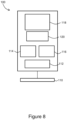
- a linear array transducer 110 is configured to transmit energy into an object to be imaged (for example, a part of the human or animal body) and to receive ultrasound echoes from the object.
- any suitable transducer may be used to receive 2D or 3D ultrasound data and may not be a linear array.
- the transducer may be a phased array, curvilinear array, or other suitable array.
- the received ultrasound echoes are digitized by an analogue to digital converter (ADC) 112.
- ADC analogue to digital converter
- the digitized ultrasound data is stored in memory 116.
- the digitized ultrasound data is processed by a processor 114 and the resulting processed data may also be stored in memory 116, or in another memory.
- the processor 114 may be configured to perform beamforming of the digitized echo data. In some embodiments, more than one processor 114 may be used.
- the ultrasound imaging apparatus 100 also includes a screen 118 for the display of ultrasound images (which results from further post-processing that is tailored to the display requirements) and one or more user input devices 120 (for example, a keyboard, mouse or trackball) for receiving input from a user of the ultrasound imaging apparatus 112, for example a sonographer.
- a screen 118 for the display of ultrasound images (which results from further post-processing that is tailored to the display requirements)
- one or more user input devices 120 for example, a keyboard, mouse or trackball
- a sonographer for example, a sonographer.
- the ultrasound imaging apparatus 100 is configured to obtain ultrasound data using the linear array transducer 110 and to process that data.
- a separate processing apparatus for example, a workstation or general purpose computer
- the organs imaged by the may include any human or animal organ, for example: organs of the digestive system including, for example, liver, pancreas; organs of the urinary system including, for example, kidneys or bladder; organs of the cardiovascular system, including the heart; any sensory organ; organ of the central nervous system, including the brain.
- the anatomical feature may include any component of the lymphatic system, including, for example, lymphatic vessels and lymph nodes.
- the anatomical feature may include any component of the cardiovascular system, including, for example, the heart, arteries, veins, capillaries, a part of the vascular bed.
- detection and classification processes performed according to certain embodiments in order to identify and determine the location of single microbubbles or multiple microbubble elements (for example, multiple microbubbles that appear to overlap in a view provided by the frame or frames in question).
- the detection and classification processes can be considered to include or comprise a segmentation process that determines the parts of the image that correspond to single or multiple microbubbles.
- a semi-automatic detection process is used in some embodiments to detect image particles (e.g. contrast elements) with a range of sizes and ensure that noise was rejected using an adaptive non-local means (NLM) filter, which has shown to work well with super-resolution ultrasound microvessel imaging.
- NLM adaptive non-local means
- the manual input of 4 parameters is used in some embodiments: the average microbubble (MB) echo intensity, the minimum, the maximum and the typical MB echo size. These may for example be roughly estimated in an initial observation of a video loop.
- the algorithm preserves the intensity of each MB signal by using of a particle probability image (PPI), a non-local mapping of the original greyscale image through the use of multi-scale Haar-like features.
- PPI particle probability image
- the resulting Haar feature image is the linear combination of the maximum value of each spatial scale at each pixel.
- the pixels with higher values may be considered as statistically significant, which means that they have a large probability of belonging to a MB rather than the background.
- the pixels of the Haar feature image are classified in two categories based on a noise threshold.
- This threshold is determined by the number of pixels in the original image that have intensity above the average noise level of the whole frame sequence creating a binary image which is used to calculate the PPI.
- the noise threshold in the first instance is adapted to the data.
- the manual input of minimum particle size is a secondary noise classifier as all particles below the minimum size are effectively considered as noise.
- the particle probability in each pixel in its binary image, within this area is the ratio of the number of pixels that have value equal to one divided by the total number of pixels of the particle area.
- a region threshold of 1/e is applied to the normalised PPI, which has unity as its maximum value, to roughly estimate the target regions.
- This enables the discrimination of the foreground and the background and generates an initial segmented image.
- the input image is convolved with a Gaussian kernel to create a Gaussian smoothed image which is used to extract the local maxima of the image. Only the local maxima points that belong to a segmented region and have particle probability value above the threshold (1/e) are preserved creating final watershed seed points. These points determine the regions that the final segmentation process is based on.
- the final detection is refined by an automatic update in the last step of the detection process.
- MB echo regions with a size below the minimum input size and input average intensity and above the maximum input size, which depended on the signal to noise ratio (SNR) of the frame sequence, may be eliminated.
- SNR signal to noise ratio
- the above process created conditions for detection based on the MB signal enhancement and enabled the automatic MB detection update from frame to frame.
- the algorithm can perform well even in low SNR environments which are common in CEUS imaging.
- Segmentation can in some cases be a key step to accurate localisation.
- Markercontrolled watershed segmentation as described, can work efficiently in optical microscopy, where the PSF of the system is known and is generally symmetric and constant in a frame sequence.
- the algorithm implements segmentation by using the gradient image of the Gaussian smoothed image, which is restricted by the dilated regions of the watershed seed points. These regions and the gradient image represent the input values of the watershed transform.
- These two input values on the one hand result in a reduction of the particle boundaries if watershed is applied to a single, separated enough, particle and on the other hand, in low SNR images, where the gradient is unreliable, restrict the segmentation up to dilated regions.
- the change in particle area does not affect the localisation accuracy as the intensity-weighted centre of mass method works well in a circular and constant PSF.
- the PSF is variable not only between different frames but also within the same frame as the acoustic field and aberrations change across the image.
- MB echoes have non-regular shapes which can make the accurate segmentation of each region important for efficient localisation.
- the gradient image is replaced by a Gaussian smoothed and inverted image as the input variable of the watershed transform. The latter can better recover the MB echo area and avoid the reduction caused by the gradient image. This can be particularly useful for MBs that have low intensity and thus low SNR as well as multiple MBs that are close to each other and were difficult to discriminate.
- CEUS differs significantly from optical microscopy. In live cell imaging accurate knowledge of the PSF permits the differentiation of particles that partially overlap in the image. The strong PSF variability in CEUS can make such techniques difficult to implement.
- the overlapping MBs can require a different processing in CEUS.
- the fact that MBs are flowing inside a branching vascular network permits the basic assumption that in a sparse MB infusion the occurrence of overlapping MBs would mostly occur in larger vessels and rarely in capillaries. This is because the MB concentration is much larger in the larger vessels.
- the overlapping MBs may be treated in the detection and segmentation process as a single event.
- the algorithm can determine the size and the neighbourhood of the detected MBs by adjusting two parameters; the Gaussian smoothing and the local maxima width. Fewer detections may occur if either the Gaussian smoothing, or the width are increased. Since in an overlapping event there may be low confidence as to whether the local maxima truly represent single MBs, the choice of larger values in the Gaussian width and the local maxima width enables a single detection.
- the possibility of overlapping MBs that are found in different vessels needs to be accommodated. In this case, the group of overlapping MBs does not travel together in the vascular bed but rather happen to be located in distances below the image resolution limit. In this case, during the frame sequence the overlapping MB echo emerges from or results in a number of single or overlapping events. For this, the birth and death of a particle within the algorithm allows for the splitting and merging of particles, which may occur in consecutive frames.
- the final segmented regions can be used for the localisation of each MB.
- An intensity-weighted centre of mass is used in certain embodiments. This is because the final segmented regions can preserve all the original information to deploy this method.
- Alternative methods include the use the full width half maximum (FWHM), a deconvolution of the PSF or the local maxima to calculate the centre of the PSF. These methods may, for example, not deploy the intensity of the segmented regions or rely heavily on the assumption that the PSF is constant.
- FWHM full width half maximum
- MB linking in consecutive frames is completed utilising the nearest neighbour method.
- a track density map and a velocity map can be generated in a pixel resolution of choice, which can be at standard resolution or super resolution.
- all the tracks may be superimposed in one figure to create a final density map.
- the value of each pixel of this map can indicate the number of tracks that passed through this pixel.
- the algorithm can provide information about the speed of the MBs and a MB velocity map can be generated. First of all the average velocity of each track can be calculated. Given that several tracks may cross within each pixel, the velocity map may be the mean of the average values of the tracks that pass through this pixel.
- Performance metrics/criteria have been calculated for synthetic and in-vivo data.
- Synthetic data The detection efficiency and localisation accuracy of the algorithm according to an embodiment was tested by means of five statistical measurements on the synthetic data. These are as follows: Root Mean Square Error (RMSE).
- Missed Events Any event from the ground truth that does not pair with a detection event, is counted as a missed event.
- Spurious Events On the other hand, all the detection result events which do not find a ground truth pair are counted as spurious events. This is a measure of detection accuracy.
- In-vivo data The accuracy and efficiency of the methodology was evaluated by comparing features on the final density maps with those identifiable on optical microscopy, OPT or OCT. Large measurements from features such as follicle cross-section area were measurement as well as smaller features such as follicle walls and vessel diameters.
- Table 1 below provides statistical results for the detection and localisation accuracy on synthetic ultrasound data (5663 single MB events in 200 frames) using the gradient and the inverted Gaussian image as the input variable of the watershed transform.
- Table 1 Gradient Inverted Gaussian Detected Events (%) 906 (16%) 5659 (99.93%) Missed Events (%) 4757 (84%) 4 (0.07%) Spurious Events 0 0 Minimum Distance (pixels) 0.01 (1.23 ⁇ m) 0 Maximum Distance (pixels) 2.73 (335.28 ⁇ m) 1.56 (191.59 ⁇ m) RMSE (pixels) 0.64 78.6 ⁇ m ⁇ ⁇ 3 0.21 25.8 ⁇ m ⁇ ⁇ 10
- Table 1 summarises differences between the two segmentation approaches, detecting 5663 single MBs on 200 synthetic frames. Better size and shape recovery of the original microbubbles led to the significant improvement in localization accuracy.
- the RMSE was 3 times lower using the inverted Gaussian (25.8 ⁇ m) compared to the gradient image (78.6 ⁇ m).
- the inverted Gaussian method there was a significant decrease of the missed events using the inverted Gaussian method to 0.07% (Table 1).
- the high occurrence of missed events using the Gradient image is explained by the removal of scatterers by the algorithm that were significantly reduced in size using the gradient image as they have size below the MB echo input size, which is set noise cancellation.
- training process 16 of Figure 1 an example implementation of the training process is now described. However, alternative training processes may be implemented or the training process may be optional.
- the user chooses an initial parameter set (corresponding to parameters D2 to D6 below) according to the density (D6) of the micro-bubbles per frame and the Signal to Noise Ratio (SNR) (D5) and the rough understanding that exists on size (D3, D4) and intensity (D2) of the microbubbles. These determine the rest of the parameters (D7 to D11).
- An automatic training of the algorithm based on a 2D Gaussian fitting distribution process is implemented in order to get the optimized parameter set for the software.
- a 2D Gaussian fitting is chosen because this fitting is closest to the shape of single microbubbles in vivo.
- the training process includes firstly, identifying microbubbles of a few frames (with the initial parameter set) following the detection process described above and the 2D Gaussian distributions are fitted to each detected microbubble and the total root mean square error (RMSE) of the fit is calculated. Then this process is repeated testing each time a different parameter combination.
- the combination that gives the smallest total RMSE is selected to be the optimised parameter combination (corresponding to parameters D2-D11) that is used for the detection, while the linking parameter (MD below) is fixed and depends on the motion of the MBs and is defined separately.
- the training process may be carried out on a subset of frame or on a separately captured training set.
- the parameter set is as follows:
Landscapes
- Health & Medical Sciences (AREA)
- Engineering & Computer Science (AREA)
- Life Sciences & Earth Sciences (AREA)
- Medical Informatics (AREA)
- Public Health (AREA)
- Physics & Mathematics (AREA)
- General Health & Medical Sciences (AREA)
- Biomedical Technology (AREA)
- Pathology (AREA)
- Radiology & Medical Imaging (AREA)
- Nuclear Medicine, Radiotherapy & Molecular Imaging (AREA)
- Veterinary Medicine (AREA)
- Surgery (AREA)
- Animal Behavior & Ethology (AREA)
- Biophysics (AREA)
- Molecular Biology (AREA)
- Heart & Thoracic Surgery (AREA)
- Computer Vision & Pattern Recognition (AREA)
- Theoretical Computer Science (AREA)
- General Physics & Mathematics (AREA)
- Primary Health Care (AREA)
- Epidemiology (AREA)
- Databases & Information Systems (AREA)
- Data Mining & Analysis (AREA)
- Hematology (AREA)
- Multimedia (AREA)
- Vascular Medicine (AREA)
- Quality & Reliability (AREA)
- Computer Graphics (AREA)
- General Engineering & Computer Science (AREA)
- Physiology (AREA)
- Ultra Sonic Daignosis Equipment (AREA)
Claims (15)
- Procédé de suivi d'un élément de contraste, mis en œuvre par ordinateur, comprenant les étapes consistant à :obtenir une séquence de trames comprenant chacune des données d'imagerie par ultrasons ou d'une autre imagerie médicale représentant une région anatomique d'un sujet humain ou animal à un moment différent respectif ;pour chaque trame, identifier une ou plusieurs portions des données d'imagerie par ultrasons ou d'une autre imagerie médicale, dans lequel les portions identifiées comprennent à la fois au moins une portion de signal d'élément de contraste unique et au moins une portion de signal d'élément de contraste multiple, chaque portion de signal d'élément de contraste unique étant représentative d'un élément de contraste et chaque portion de signal d'élément de contraste multiple étant représentative d'une pluralité d'éléments de contraste ;attribuer des données de position respectives à chacune des portions de signal d'élément de contraste uniques et attribuer des données de position respectives à chacune des portions de signal d'élément de contraste multiples ; etutiliser un modèle de liaison qui utilise au moins lesdites données de position attribuées pour lier des portions de signal d'élément de contraste uniques ou multiples représentées dans au moins l'une des trames à des portions de signal d'élément de contraste uniques ou multiples représentées dans au moins une autre des trames pour suivre ainsi un mouvement d'éléments de contraste à travers ladite région du sujet.
- Procédé selon la revendication 1, dans lequel les éléments de contraste comprennent des microbulles.
- Procédé selon la revendication 1 ou 2, dans lequel :chacune des trames représente une vue de la région du sujet, et pour au moins certaines des portions de signal d'élément de contraste multiples, la portion de signal d'élément de contraste multiple est représentative d'éléments de contraste séparés qui semblent se chevaucher selon ladite vue ;
et/ouchacune des portions de signal d'élément de contraste multiples est représentative d'éléments de contraste séparés qui apparaissent à l'avant ou à l'arrière l'un de l'autre selon ladite vue ;
et/oule procédé comprend en outre la classification pour chacune des trames des une ou plusieurs portions de signal identifiées comme soit étant une portion de signal d'élément de contraste unique soit une portion de signal d'élément de contraste multiple. - Procédé selon l'une quelconque des revendications précédentes, dans lequel le modèle de liaison est configuré pour déterminer s'il s'est ou ne s'est pas produit un évènement de fusion d'élément de contraste et/ou un évènement de dissociation d'élément de contraste et/ou un évènement de disparition d'élément de contraste et/ou un évènement de mouvement d'élément de contraste entre au moins l'une des trames et au moins une autre des trames.
- Procédé selon l'une quelconque des revendications précédentes, dans lequel :le modèle de liaison peut fonctionner pour lier au moins une portion de signal d'élément de contraste unique dans au moins l'une des trames à une portion de signal d'élément de contraste multiple dans au moins une autre ultérieure des trames ;
et/oudans lequel le modèle de liaison peut fonctionner pour lier une portion de signal d'élément de contraste multiple dans au moins l'une des trames à au moins une portion de signal d'élément de contraste unique dans au moins une autre ultérieure des trames ;
et/oule modèle de liaison peut fonctionner pour lier une portion de signal d'élément de contraste multiple représentant un premier nombre d'éléments de contraste dans au moins l'une des trames à une portion de signal d'élément de contraste multiple représentant un second nombre différent d'éléments de contraste dans au moins l'une des trames. - Procédé selon l'une quelconque des revendications précédentes, dans lequel :l'attribution de données de position à chacune des portions de signal d'élément de contraste uniques et à chacune des portions de signal d'élément de contraste multiples comprenant l'attribution d'une valeur de position unique respective à chacune des portions de signal d'élément de contraste uniques et à chacune des portions de signal d'élément de contraste multiples ;
et/oules données d'imagerie par ultrasons représentent une intensité comme une fonction de position avec une première résolution de position, l'attribution de données de position à une portion de signal d'élément de contraste est basée sur la variation d'intensité avec une position pour ladite portion de signal d'élément de contraste, et les données de position attribuées présentent une seconde résolution de position qui est supérieure à ladite première résolution de position, facultativement dans lequel la seconde résolution de position est au moins 4 fois la première résolution de position, facultativement au moins 9 fois la première résolution de position ;
et/oul'attribution de données de position à une portion de signal d'élément de contraste comprend l'ajustement d'une fonction mathématique pour déterminer une position en utilisant au moins l'une parmi : une intensité, une forme et une taille de portion de signal, facultativement dans lequel la fonction mathématique est une fonction gaussienne, en outre facultativement dans lequel la position déterminée correspond à un pic de la fonction gaussienne. - Procédé selon l'une quelconque des revendications précédentes, comprenant en outre l'attribution de données de vélocité ou de vitesse aux une ou plusieurs portions de signal.
- Procédé selon l'une quelconque des revendications précédentes, dans lequel l'identification comprend la réalisation d'un processus de segmentation pour déterminer la présence de microbulles uniques ou multiples, et facultativement le processus de segmentation comprend l'application d'au moins l'un parmi un processus d'ajustement, de filtrage et/ou de transformation, facultativement un processus de transformation par ligne de partage des eaux ;
et/oule processus de segmentation comprend la détermination de la présence de microbulles uniques et de microbulles multiples, et facultativement le processus d'ajustement, de filtrage et/ou de transformation, ou au moins un paramètre du processus d'ajustement, de filtrage et/ou de transformation, est différent pour des microbulles uniques que pour des microbulles multiples ;
et/oule processus de segmentation est réalisé sur une version modifiée des données de chaque trame, facultativement une version lissée et/ou filtrée et/ou inversée des données de chaque trame. - Procédé selon l'une quelconque des revendications précédentes, dans lequel :l'identification d'une ou de plusieurs portions des données d'imagerie par ultrasons comme étant représentatives d'un élément de contraste ou d'une pluralité d'éléments de contraste comprend l'identification de portions de signal d'élément de contraste candidates et la réalisation d'un processus de seuillage ou de filtrage pour exclure au moins certaines desdites portions de signal d'élément de contraste candidates ;
et/oupour chaque trame, l'identification d'une ou de plusieurs portions des données d'imagerie par ultrasons comme étant représentatives d'un élément de contraste ou d'une pluralité d'éléments de contraste est au moins partiellement non contrainte par le nombre de portions de données d'imagerie par ultrasons identifiées comme étant représentatives d'un élément de contraste ou d'une pluralité d'éléments de contraste pour au moins une autre des trames, de sorte que le nombre d'éléments de contraste identifiés peut être différent pour des trames différentes, facultativement de sorte que le nombre d'éléments de contraste identifiés pour au moins l'une des trames est sensiblement indépendant d'un nombre d'éléments de contraste identifiés pour au moins une autre des trames ;
et/oule procédé comprend en outre l'identification, pour au moins certaines des trames, de chacune de plus de 10, facultativement plus de 100, facultativement plus de 500, facultativement plus de 1 000 portions des données d'imagerie par ultrasons par trame comme étant représentatives d'éléments de contraste uniques ou multiples respectifs ;
et/oula séquence de trames représente une période de mesure ayant une durée entre au moins l'une parmi : 1 seconde et 10 secondes ; 10 secondes et 30 secondes ; 30 secondes et 1 minute ; de moins de 5 minutes ;
et/oula séquence de trames comprend un taux de trame dans la plage de 10 trames par seconde à 50 trames par seconde, facultativement de plus de 50 trames par seconde. - Procédé selon l'une quelconque des revendications précédentes, dans lequel :au moins certains des éléments de contraste sont présents dans des vaisseaux chez le sujet humain ou animal, et le procédé comprend l'utilisation dudit suivi dudit mouvement d'éléments de contraste à travers ladite région pour suivre les trajets d'au moins certains desdits vaisseaux ;
et/ouau moins certains des éléments de contraste sont présents à l'extérieur de vaisseaux chez le sujet humain ou animal, et le procédé comprend l'utilisation dudit suivi dudit mouvement d'éléments de contraste hors des vaisseaux ;
et/oule procédé comprend en outre l'utilisation dudit suivi pour fournir une mesure de mouvement pulsatile ou d'un autre mouvement du sujet. - Procédé selon l'une quelconque des revendications précédentes, dans lequel :le procédé comprend l'utilisation dudit suivi dudit mouvement d'éléments de contraste à travers ladite région pour suivre un passage du sang dans, hors de, ou à travers, au moins une caractéristique anatomique d'intérêt, facultativement la caractéristique anatomique comprend au moins une tumeur ou un organe ;
et/ouau moins certains des éléments de contraste sont présents dans des vaisseaux chez le sujet humain ou animal, et les vaisseaux ont une plage de tailles, et le procédé comprend, pour au moins certaines des trames, l'identification d'éléments de contraste dans des vaisseaux qui présentent une plage de différentes tailles, facultativement au moins certains desdits vaisseaux de ladite plage ayant des sections transversales et/ou des débits d'écoulement qui sont au moins 2 fois, facultativement 5 fois, facultativement 10 fois, facultativement 100 fois supérieurs à au moins un autre desdits vaisseaux ;
et/oula séquence de trames comprenant chacune des données d'imagerie par ultrasons sont obtenues par des mesures par ultrasons sur un sujet humain ou animal vivant. - Procédé selon l'une quelconque des revendications précédentes, dans lequel la liaison de portions de signal d'élément de contraste uniques ou multiples pour suivre ainsi un mouvement d'éléments de contraste comprend la formation de segments de suivi entre des trames consécutives en utilisant les données de position pour les portions de signal d'élément de contraste uniques et multiples et la jonction des segments de suivi formés pour produire une pluralité de suivis d'élément de contraste, et facultativement : la j onction des segments de suivi comprend au moins l'une parmi une fermeture, une fusion et une dissociation d'espace, facultativement sur la base d'au moins l'un parmi une taille, une distance, une intensité de signal et un sens de mouvement ;
et/ou
le procédé comprend en outre l'introduction des éléments de contraste chez le sujet, facultativement en utilisant au moins l'une parmi une perfusion en bolus ou continue. - Système de traitement d'image (100) comprenant
une ressource de traitement (114) configurée pour :recevoir une séquence de trames comprenant chacune des données d'imagerie par ultrasons ou d'une autre imagerie médicale représentant une région anatomique d'un sujet humain ou animal à un moment différent respectif ;pour chaque trame,identifier une ou plusieurs portions des données d'imagerie par ultrasons ou d'une autre imagerie médicale, dans lequel les portions identifiées comprennent à la fois au moins une portion de signal d'élément de contraste unique et au moins une portion de signal d'élément de contraste multiple, chaque portion de signal d'élément de contraste unique étant représentative d'un élément de contraste et chaque portion de signal d'élément de contraste multiple étant représentative d'une pluralité d'éléments de contraste ;attribuer des données de position respectives à chacune des portions de signal d'élément de contraste uniques et attribuer des données de position respectives à chacune des portions de signal d'élément de contraste multiples ; etutiliser un modèle de liaison qui utilise au moins lesdites données de position attribuées pour lier des portions de signal d'élément de contraste uniques ou multiples représentées dans au moins l'une des trames à des portions de signal d'élément de contraste uniques ou multiples représentées dans au moins une autre des trames pour suivre ainsi un mouvement d'éléments de contraste à travers ladite région du sujet. - Système d'imagerie comprenant :un scanner par ultrasons (110), ou un autre scanner, configuré pour réaliser un balayage d'un sujet humain ou animal pour obtenir une séquence de trames ; etun système de traitement d'image selon la revendication 13, configuré pour recevoir et traiter la séquence de trames pour suivre un mouvement d'éléments de contraste à travers une région du sujet.
- Progiciel informatique comprenant des instructions pouvant être lues par ordinateur qui peuvent être exécutées pour réaliser un procédé selon l'une quelconque des revendications 1 à 12.
Applications Claiming Priority (2)
| Application Number | Priority Date | Filing Date | Title |
|---|---|---|---|
| GBGB1716606.7A GB201716606D0 (en) | 2017-10-10 | 2017-10-10 | Tracking in ultrasound imaging |
| PCT/GB2018/052895 WO2019073227A1 (fr) | 2017-10-10 | 2018-10-10 | Suivi en imagerie ultrasonore |
Publications (3)
| Publication Number | Publication Date |
|---|---|
| EP3695378A1 EP3695378A1 (fr) | 2020-08-19 |
| EP3695378C0 EP3695378C0 (fr) | 2025-05-07 |
| EP3695378B1 true EP3695378B1 (fr) | 2025-05-07 |
Family
ID=60326923
Family Applications (1)
| Application Number | Title | Priority Date | Filing Date |
|---|---|---|---|
| EP18788835.9A Active EP3695378B1 (fr) | 2017-10-10 | 2018-10-10 | Suivi en imagerie ultrasonore |
Country Status (4)
| Country | Link |
|---|---|
| US (1) | US11944499B2 (fr) |
| EP (1) | EP3695378B1 (fr) |
| GB (1) | GB201716606D0 (fr) |
| WO (1) | WO2019073227A1 (fr) |
Families Citing this family (15)
| Publication number | Priority date | Publication date | Assignee | Title |
|---|---|---|---|---|
| EP3905960B1 (fr) * | 2019-01-03 | 2024-09-25 | Koninklijke Philips N.V. | Systèmes et procédés d'imagerie à amélioration de contraste |
| CN110458836A (zh) * | 2019-08-16 | 2019-11-15 | 深圳开立生物医疗科技股份有限公司 | 一种超声造影成像方法、装置和设备及可读存储介质 |
| CN115066196B (zh) * | 2020-02-06 | 2025-05-13 | 富士胶片株式会社 | 医用图像处理装置、内窥镜系统、医用图像处理方法及记录介质 |
| CN111598965B (zh) * | 2020-05-18 | 2023-07-14 | 南京超维景生物科技有限公司 | 超声造影图像的超分辨重建预处理方法和超分辨重建方法 |
| CN111598782B (zh) * | 2020-05-18 | 2022-05-17 | 南京超维景生物科技有限公司 | 超分辨流场重建方法及其装置 |
| US12175662B2 (en) * | 2020-09-03 | 2024-12-24 | Mayo Foundation For Medical Education And Research | Methods for extracting and quantifying diagnostic biomarkers from ultrasound microvessel images |
| US12217428B2 (en) * | 2020-09-17 | 2025-02-04 | Motilent Limited | Motion analysis of the digestive tract |
| CN116568222B (zh) * | 2020-12-17 | 2026-04-21 | 富士胶片株式会社 | 超声波诊断装置及超声波诊断装置的控制方法 |
| US12343208B2 (en) * | 2021-09-09 | 2025-07-01 | Roger Zemp | Ultrasound imaging using a bias-switchable row-column array transducer |
| US12569881B2 (en) | 2021-09-09 | 2026-03-10 | Roger Zemp | Bias-switchable ultrasonic transducer array |
| CN114463653B (zh) * | 2022-04-12 | 2022-06-28 | 浙江大学 | 一种高浓度微群泡形态识别及轨迹追踪测速方法 |
| CN116115268B (zh) * | 2023-02-14 | 2025-09-16 | 西安交通大学 | 一种新型的快速超声超分辨成像方法、系统、设备及介质 |
| EP4665237A1 (fr) * | 2023-02-15 | 2025-12-24 | Heriot-Watt University | Procédé et appareil de suivi |
| US20250143674A1 (en) * | 2023-09-27 | 2025-05-08 | Canon Medical Systems Corporation | Ultrasonic diagnostic apparatus, medical information processing apparatus, and medical information processing method |
| US12396706B2 (en) | 2023-10-04 | 2025-08-26 | Clinisonix Inc. | Synthetic phase alternating row-column transducer array |
Family Cites Families (4)
| Publication number | Priority date | Publication date | Assignee | Title |
|---|---|---|---|---|
| DE102005039685B4 (de) * | 2005-08-22 | 2007-10-11 | Siemens Ag | Verfahren zur Identifizierung eines kontrastierten Blutgefäßes in digitalen Bilddaten |
| US9913624B2 (en) * | 2013-02-28 | 2018-03-13 | Wisconsin Alumni Research Foundation | Method and apparatus for rapid acquisition of elasticity data in three dimensions |
| EP3097432B1 (fr) * | 2014-01-23 | 2022-07-06 | Supersonic Imagine | Procédé pour déterminer une caractéristique physique sur un emplacement ponctuel à l'intérieur d'un support, procédé pour déterminer une image d'un support et appareil mettant en oeuvre lesdits procédés |
| US11589840B2 (en) * | 2017-05-31 | 2023-02-28 | Mayo Foundation For Medical Education And Research | Methods for super-resolution ultrasound imaging of microvessels |
-
2017
- 2017-10-10 GB GBGB1716606.7A patent/GB201716606D0/en not_active Ceased
-
2018
- 2018-10-10 US US16/755,334 patent/US11944499B2/en active Active
- 2018-10-10 EP EP18788835.9A patent/EP3695378B1/fr active Active
- 2018-10-10 WO PCT/GB2018/052895 patent/WO2019073227A1/fr not_active Ceased
Also Published As
| Publication number | Publication date |
|---|---|
| EP3695378C0 (fr) | 2025-05-07 |
| GB201716606D0 (en) | 2017-11-22 |
| EP3695378A1 (fr) | 2020-08-19 |
| US11944499B2 (en) | 2024-04-02 |
| WO2019073227A1 (fr) | 2019-04-18 |
| US20200305840A1 (en) | 2020-10-01 |
Similar Documents
| Publication | Publication Date | Title |
|---|---|---|
| EP3695378B1 (fr) | Suivi en imagerie ultrasonore | |
| US8958618B2 (en) | Method and system for identification of calcification in imaged blood vessels | |
| CN105913432B (zh) | 基于ct序列图像的主动脉提取方法及装置 | |
| US9119559B2 (en) | Method and system of generating a 3D visualization from 2D images | |
| Ghavami et al. | Quantification of morphological features in non-contrast-enhanced ultrasound microvasculature imaging | |
| Sameh et al. | Narrowed coronary artery detection and classification using angiographic scans | |
| Özdemir et al. | Three-dimensional visualization and improved quantification with super-resolution ultrasound imaging-validation framework for analysis of microvascular morphology using a chicken embryo model | |
| Kamra et al. | Performance comparison of image segmentation techniques for lung nodule detection in CT images | |
| Gu et al. | Ultrafast ultrasound localization microscopy by conditional generative adversarial network | |
| Vasanthselvakumar et al. | Detection and classification of kidney disorders using deep learning method | |
| Alzahrani et al. | Deep learning approach for breast ultrasound image segmentation | |
| Edmund et al. | Artificial intelligence-assisted Internet of Medical Things enabling medical image processing | |
| Sankaranarayanan et al. | Detection of oral tumor based on marker controlled watershed algorithm | |
| US12315141B2 (en) | Systems and methods for quantifying vessel features in ultrasound doppler images | |
| Anwar et al. | Segmentation of liver tumor for computer aided diagnosis | |
| Vashishtha et al. | Nerve segmentation in ultrasound images | |
| Almi'ani et al. | Automatic segmentation algorithm for brain MRA images | |
| Kulathilake et al. | Region growing segmentation method for extracting vessel structures from coronary cine-angiograms | |
| Saénz et al. | Brain hematoma computational segmentation | |
| Gayanga et al. | Detecting and Capturing the Intensity of a Brain Tumor using MRI Images | |
| Bukenya et al. | 3D segmentation of the whole heart vasculature using improved multi-threshold Otsu and white top-hat scale space hessian based vessel filter | |
| Zimmer et al. | Image segmentation in obstetrics and gynecology | |
| Fu et al. | A new automatic segmentation algorithm for carotid artery ultrasound images | |
| Reeja et al. | A study on detection and segmentation of ischemic stroke in MRI and CT images | |
| Bautista et al. | Feasibility of deep learning-based cancer detection in ultrasound microvascular images |
Legal Events
| Date | Code | Title | Description |
|---|---|---|---|
| STAA | Information on the status of an ep patent application or granted ep patent |
Free format text: STATUS: UNKNOWN |
|
| STAA | Information on the status of an ep patent application or granted ep patent |
Free format text: STATUS: THE INTERNATIONAL PUBLICATION HAS BEEN MADE |
|
| PUAI | Public reference made under article 153(3) epc to a published international application that has entered the european phase |
Free format text: ORIGINAL CODE: 0009012 |
|
| STAA | Information on the status of an ep patent application or granted ep patent |
Free format text: STATUS: REQUEST FOR EXAMINATION WAS MADE |
|
| 17P | Request for examination filed |
Effective date: 20200415 |
|
| AK | Designated contracting states |
Kind code of ref document: A1 Designated state(s): AL AT BE BG CH CY CZ DE DK EE ES FI FR GB GR HR HU IE IS IT LI LT LU LV MC MK MT NL NO PL PT RO RS SE SI SK SM TR |
|
| AX | Request for extension of the european patent |
Extension state: BA ME |
|
| DAV | Request for validation of the european patent (deleted) | ||
| DAX | Request for extension of the european patent (deleted) | ||
| RIN1 | Information on inventor provided before grant (corrected) |
Inventor name: SBOROS, VASSILIS Inventor name: LU, WEIPING Inventor name: WILSON, RHODRI Inventor name: KANOULAS, EVANGELOS |
|
| STAA | Information on the status of an ep patent application or granted ep patent |
Free format text: STATUS: EXAMINATION IS IN PROGRESS |
|
| 17Q | First examination report despatched |
Effective date: 20220408 |
|
| GRAP | Despatch of communication of intention to grant a patent |
Free format text: ORIGINAL CODE: EPIDOSNIGR1 |
|
| STAA | Information on the status of an ep patent application or granted ep patent |
Free format text: STATUS: GRANT OF PATENT IS INTENDED |
|
| RIC1 | Information provided on ipc code assigned before grant |
Ipc: G16H 50/30 20180101ALI20241122BHEP Ipc: A61B 8/08 20060101ALI20241122BHEP Ipc: A61B 8/06 20060101ALI20241122BHEP Ipc: A61B 8/00 20060101ALI20241122BHEP Ipc: G06T 7/246 20170101AFI20241122BHEP |
|
| INTG | Intention to grant announced |
Effective date: 20241206 |
|
| GRAS | Grant fee paid |
Free format text: ORIGINAL CODE: EPIDOSNIGR3 |
|
| GRAA | (expected) grant |
Free format text: ORIGINAL CODE: 0009210 |
|
| STAA | Information on the status of an ep patent application or granted ep patent |
Free format text: STATUS: THE PATENT HAS BEEN GRANTED |
|
| AK | Designated contracting states |
Kind code of ref document: B1 Designated state(s): AL AT BE BG CH CY CZ DE DK EE ES FI FR GB GR HR HU IE IS IT LI LT LU LV MC MK MT NL NO PL PT RO RS SE SI SK SM TR |
|
| REG | Reference to a national code |
Ref country code: GB Ref legal event code: FG4D |
|
| REG | Reference to a national code |
Ref country code: CH Ref legal event code: EP |
|
| REG | Reference to a national code |
Ref country code: DE Ref legal event code: R096 Ref document number: 602018081760 Country of ref document: DE |
|
| REG | Reference to a national code |
Ref country code: IE Ref legal event code: FG4D |
|
| U01 | Request for unitary effect filed |
Effective date: 20250602 |
|
| U07 | Unitary effect registered |
Designated state(s): AT BE BG DE DK EE FI FR IT LT LU LV MT NL PT RO SE SI Effective date: 20250610 |
|
| PG25 | Lapsed in a contracting state [announced via postgrant information from national office to epo] |
Ref country code: ES Free format text: LAPSE BECAUSE OF FAILURE TO SUBMIT A TRANSLATION OF THE DESCRIPTION OR TO PAY THE FEE WITHIN THE PRESCRIBED TIME-LIMIT Effective date: 20250507 |
|
| PG25 | Lapsed in a contracting state [announced via postgrant information from national office to epo] |
Ref country code: NO Free format text: LAPSE BECAUSE OF FAILURE TO SUBMIT A TRANSLATION OF THE DESCRIPTION OR TO PAY THE FEE WITHIN THE PRESCRIBED TIME-LIMIT Effective date: 20250807 Ref country code: GR Free format text: LAPSE BECAUSE OF FAILURE TO SUBMIT A TRANSLATION OF THE DESCRIPTION OR TO PAY THE FEE WITHIN THE PRESCRIBED TIME-LIMIT Effective date: 20250808 |
|
| PG25 | Lapsed in a contracting state [announced via postgrant information from national office to epo] |
Ref country code: PL Free format text: LAPSE BECAUSE OF FAILURE TO SUBMIT A TRANSLATION OF THE DESCRIPTION OR TO PAY THE FEE WITHIN THE PRESCRIBED TIME-LIMIT Effective date: 20250507 |
|
| U20 | Renewal fee for the european patent with unitary effect paid |
Year of fee payment: 8 Effective date: 20250909 |
|
| PGFP | Annual fee paid to national office [announced via postgrant information from national office to epo] |
Ref country code: GB Payment date: 20250821 Year of fee payment: 8 |
|
| PG25 | Lapsed in a contracting state [announced via postgrant information from national office to epo] |
Ref country code: HR Free format text: LAPSE BECAUSE OF FAILURE TO SUBMIT A TRANSLATION OF THE DESCRIPTION OR TO PAY THE FEE WITHIN THE PRESCRIBED TIME-LIMIT Effective date: 20250507 |
|
| PG25 | Lapsed in a contracting state [announced via postgrant information from national office to epo] |
Ref country code: RS Free format text: LAPSE BECAUSE OF FAILURE TO SUBMIT A TRANSLATION OF THE DESCRIPTION OR TO PAY THE FEE WITHIN THE PRESCRIBED TIME-LIMIT Effective date: 20250807 |
|
| PG25 | Lapsed in a contracting state [announced via postgrant information from national office to epo] |
Ref country code: IS Free format text: LAPSE BECAUSE OF FAILURE TO SUBMIT A TRANSLATION OF THE DESCRIPTION OR TO PAY THE FEE WITHIN THE PRESCRIBED TIME-LIMIT Effective date: 20250907 |
|
| PG25 | Lapsed in a contracting state [announced via postgrant information from national office to epo] |
Ref country code: SM Free format text: LAPSE BECAUSE OF FAILURE TO SUBMIT A TRANSLATION OF THE DESCRIPTION OR TO PAY THE FEE WITHIN THE PRESCRIBED TIME-LIMIT Effective date: 20250507 |
|
| PG25 | Lapsed in a contracting state [announced via postgrant information from national office to epo] |
Ref country code: CZ Free format text: LAPSE BECAUSE OF FAILURE TO SUBMIT A TRANSLATION OF THE DESCRIPTION OR TO PAY THE FEE WITHIN THE PRESCRIBED TIME-LIMIT Effective date: 20250507 |
|
| PG25 | Lapsed in a contracting state [announced via postgrant information from national office to epo] |
Ref country code: SK Free format text: LAPSE BECAUSE OF FAILURE TO SUBMIT A TRANSLATION OF THE DESCRIPTION OR TO PAY THE FEE WITHIN THE PRESCRIBED TIME-LIMIT Effective date: 20250507 |
|
| PLBE | No opposition filed within time limit |
Free format text: ORIGINAL CODE: 0009261 |
|
| STAA | Information on the status of an ep patent application or granted ep patent |
Free format text: STATUS: NO OPPOSITION FILED WITHIN TIME LIMIT |
|
| REG | Reference to a national code |
Ref country code: CH Ref legal event code: L10 Free format text: ST27 STATUS EVENT CODE: U-0-0-L10-L00 (AS PROVIDED BY THE NATIONAL OFFICE) Effective date: 20260318 |
|
| 26N | No opposition filed |
Effective date: 20260210 |
|
| U1N | Appointed representative for the unitary patent procedure changed after the registration of the unitary effect |
Representative=s name: MARKS & CLERK LLP; GB |