EP3997665B1 - Verfahren zur erzeugung von oberflächendaten und vorrichtung hierzu - Google Patents
Verfahren zur erzeugung von oberflächendaten und vorrichtung hierzu Download PDFInfo
- Publication number
- EP3997665B1 EP3997665B1 EP20739954.4A EP20739954A EP3997665B1 EP 3997665 B1 EP3997665 B1 EP 3997665B1 EP 20739954 A EP20739954 A EP 20739954A EP 3997665 B1 EP3997665 B1 EP 3997665B1
- Authority
- EP
- European Patent Office
- Prior art keywords
- node
- projection images
- auxiliary points
- density
- detector unit
- Prior art date
- Legal status (The legal status is an assumption and is not a legal conclusion. Google has not performed a legal analysis and makes no representation as to the accuracy of the status listed.)
- Active
Links
Images

Classifications
-
- G—PHYSICS
- G06—COMPUTING OR CALCULATING; COUNTING
- G06T—IMAGE DATA PROCESSING OR GENERATION, IN GENERAL
- G06T12/00—Tomographic reconstruction from projections
- G06T12/30—Image post-processing, e.g. metal artefact correction
-
- G—PHYSICS
- G06—COMPUTING OR CALCULATING; COUNTING
- G06T—IMAGE DATA PROCESSING OR GENERATION, IN GENERAL
- G06T17/00—Three-dimensional [3D] modelling for computer graphics
- G06T17/20—Finite element generation, e.g. wire-frame surface description, tesselation
- G06T17/205—Re-meshing
-
- G—PHYSICS
- G06—COMPUTING OR CALCULATING; COUNTING
- G06T—IMAGE DATA PROCESSING OR GENERATION, IN GENERAL
- G06T2211/00—Image generation
- G06T2211/40—Computed tomography
- G06T2211/416—Exact reconstruction
-
- G—PHYSICS
- G06—COMPUTING OR CALCULATING; COUNTING
- G06T—IMAGE DATA PROCESSING OR GENERATION, IN GENERAL
- G06T2211/00—Image generation
- G06T2211/40—Computed tomography
- G06T2211/424—Iterative
Definitions
- the invention relates to a method for generating surface data of an object with projection images which were acquired by computer tomographic measurement of the object positioned in the beam path between a radiation source and a detector unit, as well as a device suitable for carrying out the method.
- Measuring devices for the computed tomographic measurement of an object are now increasingly used in industrial environments for the inspection of workpieces.
- a typical measuring device for computed tomography measurement of an object includes at least one radiation source (source of invasive radiation, for example an X-ray source), a positioning device for positioning and moving the object (manipulation system, for example a turntable) and a detector unit (for example a flat panel detector).
- source of invasive radiation for example an X-ray source
- positioning device for positioning and moving the object for example a turntable
- detector unit for example a flat panel detector
- the object is positioned in the beam path between the radiation source and the detector unit, for example using the positioning device.
- the invasive radiation from the radiation source is attenuated to varying degrees when it penetrates the object.
- the detector unit records data (projection images) that represent a two-dimensional image of the object.
- the object is moved to a different position using the positioning device and further data is recorded.
- it is common to record data in up to several hundred different positions of the object, for example by placing the object on a turntable and rotating it by a specified angle between recordings.
- a reconstruction algorithm can be used to calculate a volume data set from the projection images that describes the object in three dimensions.
- the volume data is made up of a large number of individual volume elements, which are often referred to as voxels. Each voxel can store information about the material density of this volume element, among other things.
- the different density data stored in each voxel are represented, for example, by different gray values.
- volume data can be converted into surface data.
- STL meshes surface meshes
- the surface can be defined as the boundary between corresponding areas.
- the surfaces can be defined as the interfaces between the material of the measurement object and the surrounding material (air).
- staircase artifacts often occur when generating surface data based on volume data. This means that even in reality flat material boundaries have a step-like structure, since the calculation is based on the volume elements of the voxel model.
- Step III) can be carried out several times to further optimize the surface data. Preferably, it is repeated until a predefined termination criterion is reached.
- Step III) is repeated for an arbitrarily defined set of nodes of the surface network.
- the defined set can include only one, several or all nodes of the surface network.
- steps a) to c) are first carried out several times for one node or until the termination criterion is met and only then is process step III) started for another node, or whether execution takes place alternately for different nodes or even simultaneously.
- step I) a volume model is reconstructed in the form of a 3D grid of gray values from the projection images of a computed tomography measurement.
- the computed tomography measurement can be carried out as a real measurement. However, it is also conceivable to simulate the computed tomography measurement using a computer.
- the filtered back-projection (FBP) method can be used to create the volume model.
- Gray values that reflect the density of the material can then be stored in the individual voxels of the volume model.
- step II initial surface data is determined using a suitable volume import procedure based on the volume model from step I).
- the surface data is advantageously a surface mesh that has a polygonal surface. A large number of triangles are often used for this purpose, which meet at nodes Ki. However, the method is not restricted to the use of triangles.
- step III the surface data are optimized by changing the positions P(Ki) of one or more nodes Ki.
- auxiliary points Hj (Ki) are defined outside the surface data for a node Ki.
- the density of the material, or a gray value representing the density, is determined at these three-dimensional auxiliary points Hj (Ki), and a new position P ⁇ (Ki) is determined for a node from this.
- This reconstruction will usually require more computing power and therefore more time than interpolating the density or gray values of neighboring nodes, but direct reconstruction usually provides more accurate values.
- the usual assumptions in the interpolation process such as the assumption of a linear density change, can be omitted during reconstruction.
- auxiliary points Hj (Ki) used can be defined in different ways.
- auxiliary points Hj (Ki) of a node Ki are selected along a normal direction of the node Ki.
- n auxiliary points can be selected that are, for example, an m-fold distance of a voxel length from the node. m can not only take on integer values.
- the auxiliary points can also be selected along another function curve. Even a free choice of the auxiliary points in a surrounding volume of the node is conceivable. This free choice can be made either manually by a user or automatically, for example via a suitable computer-implemented random function.
- a new position P ⁇ (Ki) for the corresponding node Ki can be determined on the basis of the gray or density values thus obtained at the auxiliary points Hj (Ki).
- the surface network also changes accordingly.
- one embodiment provides for an additional step to be carried out between steps II) and III), in which the first surface network is pre-optimized by interpolating the density or gray values at selected auxiliary points based on the density and gray values of neighboring nodes that were determined in the volume import process. This determines changed positions for the nodes of the surface network.
- method step III is then applied to the pre-optimized surface data.
- the method can also be used to determine object surfaces in sectional images.
- the first volume model created in step I can be aligned with a plane
- the volume model created by the cut then takes the place of the original first volume model for the further execution of the process, so that you can then continue with step II.
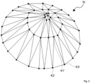
- Figure 1 shows an example surface mesh N of a section of an object.
- the object is made of one material, so that the surface to be determined in this example is the interface between the object material and air.
- the method can also be applied to interfaces between other materials.
- the interior of the cone therefore consists of the material of the object.
- the surface mesh N shown illustrates a surface that was created using a volume import procedure from measurement data (projection images) of a computed tomography survey.
- the surface is described using a large number of triangles that meet at nodes Ki.
- the Figure 1 As an example, three of the nodes K1, K2 and K3 are marked with a label. The nodes K1, K2 and K3 are located at a position P(K1), P(K2), P(K3).
- Figure 2 shows a schematic representation of the conical surface area after an iterative surface optimization has taken place using the projection images.
- the nodes K1, K2 and K3 are no longer at the original positions P(K1), P(K2), P(K3) from Figure 1 , but at the changed positions P ⁇ (K1), P ⁇ (K2) and P ⁇ (K3) and therefore designated here with the designations K1', K2' and K3'.
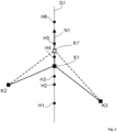
- a normal direction was determined for the node point K1, which is illustrated by the arrow N1.
- Auxiliary points H1 (K1), H2 (K1), H3 (K1), H4 (K1), H5 (K1) and H6 (K1) are defined along a straight line G1 that runs in the normal direction. Since this figure only refers to the node point K1, the auxiliary points are simply referred to as H1 to H6.
- values are determined from the projection images of a computed tomography survey using an arbitrary reconstruction algorithm, which represent the density of the material of the object at these points.
- an optimized position P (K1) can then be determined.
- auxiliary points H1 and H2 are located inside the object because they lie in the negative direction along the normal G1.
- the auxiliary points H5 and H6 are assumed to be outside the object. This means that, for example, the maximum density at the two points H1 and H2 can be assumed to be the density of the object material and the minimum density of the auxiliary points H5 and H6 can be assumed to be the density of the environment.
- the determined density values at the auxiliary points H3 and H4 can now be used to define a position along the normal at which the material transition is assumed. This determined position is assigned to the node point K1 as its changed position P'(K1) and the node point is marked in its new position with K1' in the figure.
- Figure 3 For example, the connecting lines from node K1 to neighboring nodes K2 and K3 are shown as solid lines. After the position of node K1 has been optimized, the dashed connecting lines to the neighboring nodes K2 and K3 result for this optimized position (K1').
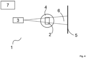
- Figure 4 shows a schematic structure of an exemplary embodiment of a device 1 for computed tomographic measurement of an object 2 and for carrying out a method for generating surface data of an object 2.
- the device 1 has a radiation source 3 (source of invasive radiation, for example an X-ray source), a positioning device 4 for positioning and moving the object 2 (manipulation system, for example a turntable) and a detector unit 5 (for example a flat panel detector).
- a radiation source 3 source of invasive radiation, for example an X-ray source
- a positioning device 4 for positioning and moving the object 2 (manipulation system, for example a turntable)
- a detector unit 5 for example a flat panel detector.
- the object In order to measure an object 2 using computer tomography, the object is positioned in the beam path 6 between the radiation source 3 and the detector unit 5, for example using the positioning device 4. Projection images are recorded in different positions of the object 2 using the detector unit 5, for example by rotating the object 2 by a predetermined angle between the recordings using the turntable 4.
- the evaluation unit 7 is suitable for executing suitable program code means in order to implement a method for Generation of surface data of an object 2 with projection images which were acquired by computer tomographic measurement of the object 2 positioned in the beam path 6 between the radiation source 3 and the detector unit 5.
- the embodiment shown here with a separate evaluation unit 7 is exemplary. Other embodiments are possible.
- the evaluation unit 7 can also be integrated into the device 1.
- the evaluation unit 7 is advantageously integrated into a control unit that is suitable for controlling the computer tomographic measurement.
Landscapes
- Physics & Mathematics (AREA)
- Engineering & Computer Science (AREA)
- General Physics & Mathematics (AREA)
- Theoretical Computer Science (AREA)
- Computer Graphics (AREA)
- Geometry (AREA)
- Software Systems (AREA)
- Analysing Materials By The Use Of Radiation (AREA)
- Apparatus For Radiation Diagnosis (AREA)
Description
- Die Erfindung betrifft ein Verfahren zur Erzeugung von Oberflächendaten eines Objektes mit Projektionsbildern, die durch computertomografische Vermessung des in den Strahlengang zwischen einer Strahlungsquelle und einer Detektoreinheit positionierten Objektes erfasst wurden, sowie eine zur Durchführung des Verfahrens geeignete Vorrichtung.
- Messeinrichtungen zur computertomografischen Vermessung eines Objektes kommen inzwischen verstärkt im industriellen Umfeld zur Prüfung von Werkstücken zum Einsatz.
- Eine typische Messeinrichtung zur computertomografischen Vermessung eines Objektes beinhaltet dabei zumindest eine Strahlungsquelle (Quelle invasiver Strahlung, zum Beispiel eine Röntgenquelle), eine Positionierungsvorrichtung zur Positionierung und Bewegung des Objektes (Manipulationssystem, beispielsweise ein Drehtisch) und eine Detektoreinheit (beispielsweise ein Flat-Panel-Detektor).
- Um ein Objekt computertomografisch zu vermessen, wird dieses beispielsweise mit Hilfe der Positionierungsvorrichtung im Strahlengang zwischen der Strahlungsquelle und der Detektoreinheit positioniert. Je nach Material und Materialstärke wird die invasive Strahlung der Strahlungsquelle unterschiedlich stark beim Durchdringen des Objektes abgeschwächt. Die Detektoreinheit erfasst Daten (Projektionsbilder), die ein zweidimensionales Abbild des Objektes repräsentieren. Das Objekt wird mit Hilfe der Positionierungsvorrichtung in eine andere Position gebracht und es werden weitere Daten aufgenommen. Zur Vermessung eines Objektes ist es üblich, Daten in bis zu mehreren hundert unterschiedlichen Positionen des Objektes aufzunehmen, beispielsweise indem sich das Objekt auf einem Drehtisch befindet und zwischen den Aufnahmen um einen vorgegebenen Winkel rotiert.
- Aus den Projektionsbildern kann mit Hilfe eines Rekonstruktionsalgorithmus ein Volumendatensatz berechnet werden, der das Objekt dreidimensional beschreibt. Die Volumendaten setzen sich dabei aus einer Vielzahl einzelner Volumenelemente zusammen, die häufig auch als Voxel bezeichnet werden. In jedem Voxel kann unter anderem auch die Information über eine Materialdichte dieses Volumenelementes gespeichert sein. Die unterschiedlichen Dichtedaten, die in jedem Voxel gespeichert sind, werden beispielsweise durch unterschiedliche Grauwerte dargestellt.
- Um in der Messtechnik übliche Auswertemethoden einsetzen zu können, wie beispielsweise Form- und Maßanalysen oder Soll-Ist-Vergleiche, ist es vorteilhaft, die Volumendaten in Oberflächendaten umzuwandeln. Beispielsweise können unterschiedliche Materialien eines Objekts dabei als separate Oberflächennetze (STL-Netze) dargestellt werden. So lassen sich auch interne Strukturen für die Analyse nutzen.
- Zur Erstellung der Oberflächendaten sind bereits Verfahren, wie der Marching-Cube-Algorithmus, bekannt.
- Beispielsweise unter der Annahme, dass unterschiedliche Materialen zu unterschiedlichen Abschwächungen der invasiven Strahlung führen und damit zu anderen Messwerten in den einzelnen Volumenelementen, kann die Oberfläche als die Grenze zwischen entsprechenden Bereichen definiert werden. Selbst bei einfachen Messobjekten, die aus einem einheitlichen Material bestehen, können die Oberflächen als die Grenzflächen vom Material des Messobjektes zum Umgebungsmaterial (Luft) bestimmt werden.
- Als Oberflächendaten seien im Folgenden die Daten zu verstehen, die Oberflächen eines Objektes beschreiben, beispielsweise polygonale Oberflächennetze. Als Oberflächen des Objektes können nicht nur die Grenzflächen zwischen dem Objekt und der Umgebung, beispielsweise Luft, verstanden werden, sondern auch Grenzflächen innerhalb des Objektes zwischen unterschiedlichen Dichtebereichen, also zum Beispiel unterschiedlichen Materialien.
- Bei herkömmlichen Verfahren kommt es bei der Erzeugung von Oberflächendaten basierend auf den Volumendaten häufig zu sogenannten Treppenartefakten. Das heißt, selbst in der Realität ebene Materialgrenzen weisen eine treppenförmige Struktur auf, da der Berechnung die Volumenelemente des Voxel-Modells zugrunde liegen.
- Yukie Nagai, Yutaka, Ohtake, und Hiromasa Suzuki: Accurate surface extraction on CT volume using analytical gradient of FDK formula, in: 9th Conference on Industrical Computed Tomography, Padova, Italien, 13.02.2019, Seiten 1 bis 8 beschreibt ein Verfahren zur Optimierung von Isoflächen anhand von computertomographisch ermittelten Werten an dreidimensionalen Punkten eines Objektes. Aus der visuellen Darstellung der CT-Rohdaten (Sinogram) wird ein CT-Volumen erstellt, aus dem eine Isofläche extrahiert wird. Für jeden Knotenpunkt des Netzes werden Gradientenwerte in der Richtung des Gradienten des CT-Wertes ermittelt. Die Knotenpunkte werden in Richtung des größten absoluten Gradientenwertes bewegt. Damit wird die Isofläche optimiert.
- Aufgabe der vorliegenden Erfindung ist es, ein verbessertes Verfahren zu schaffen, um aus den Messdaten einer computertomografischen Messung Oberflächendaten zu erzeugen.
- Diese Aufgabe wird mit einem Verfahren mit den Merkmalen des Anspruchs 1 und einer Vorrichtung mit den Merkmalen des Anspruchs 7 gelöst. Vorteilhafte Ausführungsformen sind in den Unteransprüchen beschrieben.
- Es wird vorgeschlagen, bei der Oberflächenfindung nicht nur die Volumendaten zu verwenden, sondern auch die Projektionsbilder für die Berechnung der Oberflächenpunkte mit einzubeziehen.
- Das Verfahren umfasst die folgenden Schritte:
- I) Erstellen eines ersten Volumenmodells mit den Projektionsbildern;
- II) Erzeugen eines ersten Oberflächennetzes mit Knotenpunkten basierend auf dem Volumenmodell;
- III) Optimieren der Oberflächen des Oberflächennetzes unter Zuhilfenahme von mit der Detektoreinheit erfassten Projektionsbildern.
- Erfindungsgemäß umfasst der Schritt III) dabei die folgenden Schritte:
- a) Festlegen von Hilfspunkten zu einem Knotenpunkt des Oberflächennetzes
- b) erneute Rekonstruktion an den Hilfspunkten auf Basis der Projektionsbilder
- c) Auswerten der Rekonstruktion an den Hilfspunkten und Erzeugung einer angepassten Position des Knotenpunktes des Oberflächennetzes.
- Der Schritt III) kann dabei mehrfach ausgeführt werden, um die Oberflächendaten weiter zu optimieren. Bevorzugt wird er so oft wiederholt, bis ein vordefiniertes Abbruchkriterium erreicht ist.
- Der Schritt III) wird für eine beliebig definierte Menge an Knotenpunkten des Oberflächennetzes wiederholt. Die definierte Menge kann dabei nur einen, mehrere oder auch alle Knotenpunkte des Oberflächennetzes umfassen.
- Auch ist es unerheblich, ob die Schritte a) bis c) erst für einen Knotenpunkt mehrfach oder bis zum Abbruchkriterium durchgeführt werden und erst dann der Verfahrensschritt III) für einen weiteren Knotenpunkt gestartet wird, oder ob eine Ausführung wechselnd für verschiedene Knotenpunkte oder sogar gleichzeitig erfolgt.
- Zur Vorbereitung wird in Schritt I) ein Volumenmodell in Form eines 3D-Rasters an Grauwerten aus den Projektionsbildern einer computertomografischen Vermessung rekonstruiert. Die computertomografische Vermessung kann dabei als reale Messung durchgeführt werden. Es ist aber auch denkbar, die computertomografische Vermessung rechnergestützt zu simulieren.
- Beispielsweise kann zum Erstellen des Volumenmodells die Methode der gefilterten Rückprojektion (filtered back-projection (FBP)) zum Einsatz kommen. In den einzelnen Voxeln des Volumenmodells können dann Grauwerte gespeichert sein, die die Dichte des Materials widerspiegeln.
- In Schritt II) werden mit Hilfe eines geeigneten Volumenimportverfahrens basierend auf dem Volumenmodell aus Schritt I) erste Oberflächendaten bestimmt. Die Oberflächendaten sind vorteilhafterweise ein Oberflächennetz, das eine polygonale Oberfläche darstellt. Häufig wird dazu eine Vielzahl von Dreiecken verwendet, die an Knotenpunkten Ki aneinander treffen. Das Verfahren ist aber nicht auf die Verwendung von Dreiecken eingeschränkt.
- Ein Beispiel für ein mögliches Volumenimportverfahren ist der Marching-Cube-Algorithmus.
- In Schritt III) werden die Oberflächendaten durch eine Veränderung der Positionen P(Ki) einer oder mehrerer Knotenpunkte Ki optimiert. Zur Bestimmung der veränderten Knotenpunktposition P(Ki) werden zu einem Knotenpunkt Ki Hilfspunkte Hj (Ki) außerhalb der Oberflächendaten definiert. An diesen dreidimensionalen Hilfspunkten Hj (Ki) wird die Dichte des Materials, bzw. eines die Dichte repräsentierenden Grauwertes, bestimmt und daraus eine neue Position P`(Ki) für einen Knotenpunkt festgelegt.
- Bereits bekannt sind Verfahren, die die Dichte bzw. den Grauwert an einem Punkt, also beispielsweise einem Hilfspunkt, aus den Dichte- bzw. Grauwerten von benachbarten Knotenpunkten interpolieren. Diese benachbarten Knotenpunkte und ihre Dichte- bzw. Grauwerte stammen dabei beispielsweise aus einem Marching-Cube-Verfahren. Dabei pflanzen sich Ungenauigkeiten, die bei der Erstellung des Volumenmodells in Schritt I sowie des Volumenimportverfahrens in Schritt II) vorhanden sind, weiter fort. Das erfindungsgemäße Verfahren setzt daher an dieser Stelle an den ausgewählten Hilfspunkten Hj (Ki) auf eine Rekonstruktion auf Basis der Messdaten, das heißt die Dichte- bzw. Grauwerte werden direkt an den Hilfspunkten Hj (Ki) aus den Messdaten (Projektionsbildern) berechnet, beispielsweise mittels gefilterter Rückprojektion (FBP).
- Üblicherweise wird diese Rekonstruktion einen höheren Rechenaufwand und damit einen höheren Zeitaufwand hervorrufen als eine Interpolation der Dichte- bzw. Grauwerte von benachbarten Knotenpunkten, dafür liefert die direkte Rekonstruktion aber in der Regel genauere Werte. Beispielsweise können bei der Rekonstruktion die im Interpolationsverfahren üblichen Annahmen, wie beispielsweise die Annahme einer linearen Dichteänderung, entfallen.
- Die verwendeten Hilfspunkte Hj (Ki) können auf verschiedene Weise definiert werden.
- Besonders vorteilhaft ist es, wenn die Hilfspunkte Hj (Ki) eines Knotenpunktes Ki entlang einer Normalen-Richtung des Knotenpunktes Ki gewählt werden. Beispielsweise kann eine Anzahl von n Hilfspunkten gewählt werden, die beispielsweise ein m-faches einer Voxellänge vom Knotenpunkt entfernt liegen. m kann dabei nicht nur ganzzahlige Werte annehmen.
- Statt der Auswahl der Hilfspunkte entlang einer Normalen-Richtung können die Hilfspunkte aber auch entlang einer anderen Funktionskurve gewählt werden. Selbst eine freie Wahl der Hilfspunkte in einem Umgebungsvolumen des Knotenpunktes ist denkbar. Diese freie Wahl kann dabei sowohl manuell durch einen Anwender erfolgen als auch automatisiert beispielsweise über eine geeignete computerimplementierte Zufallsfunktion.
- Ist die Rekonstruktion an den Hilfspunkten Hj (Ki) erfolgt, so kann auf Basis der damit vorliegenden Grau- bzw. Dichtewerte an den Hilfspunkten Hj (Ki) eine neue Position P`(Ki) für den dazu gehörenden Knotenpunkt Ki bestimmt werden.
- Durch die Änderung der Position eines Knotenpunktes ändert sich entsprechend auch das Oberflächennetz.
- Zur Beschleunigung des Verfahrens ist es in einer Ausführungsform vorgesehen, einen zusätzlichen Schritt zwischen den Schritten II) und III) durchzuführen, in dem das erste Oberflächennetz voroptimiert wird, indem an gewählten Hilfspunkten die Dichte- bzw. Grauwerte basierend auf den Dichte- und Grauwerten von benachbarten Knotenpunkten interpoliert werden, die im Volumenimportverfahren ermittelt wurden. Damit werden geänderte Positionen für die Knotenpunkte des Oberflächennetztes bestimmt. Nach der Voroptimierung wird dann der Verfahrensschritt III) auf die voroptimierten Oberflächendaten angewendet.
- Vorteilhafterweise kann das Verfahren auch verwendet werden, um Objektoberflächen in Schnittbildern zu bestimmen. Dazu kann in einem Zwischenschritt das in Schritt I erstellte erste Volumenmodell mit einer Ebene geschnitten werden. Das durch den Schnitt entstandene Volumenmodell tritt dann für die weitere Ausführung des Verfahrens an die Stelle des ursprünglichen ersten Volumenmodells, sodass danach mit Schritt II fortgefahren werden kann.
- Die Erfindung wird nachfolgend anhand von nicht einschränkenden Ausführungsbeispielen mit den beigefügten Zeichnungen näher erläutert. Es zeigt:
- Figur 1
- - schematische Darstellung einer Teils einer Objektoberfläche vor einer Optimierung;
- Figur 2
- - schematische Darstellung einer Teils einer Objektoberfläche nach einer Optimierung;
- Figur 3
- - Veranschaulichung der Positionsänderung eines Knotenpunktes im Zuge der Optimierung;
- Figur 4
- - schematische Darstellung einer beispielhaften Vorrichtung zur computertomografischen Vermessung eines Objektes und zum Erzeugen von Oberflächendaten.
-
Figur 1 zeigt ein beispielhaftes Oberflächennetz N eines Ausschnittes eines Objektes. Das Objekt sei zur Vereinfachung aus einem Material, sodass die in diesem Beispiel zu bestimmende Oberfläche die Grenzfläche von Objektmaterial zu Luft ist. Das Verfahren ist aber auch auf Grenzflächen zwischen anderen Materialien anwendbar. - Dargestellt ist ein kegelförmiger Oberflächenbereich, der aus dem Objekt herausragt. Das Kegelinnere besteht also aus dem Material des Objektes.
- Das dargestellte Oberflächennetz N veranschaulicht eine Oberfläche, die mit einem Volumenimportverfahren aus Messdaten (Projektionsbildern) einer computertomografischen Vermessung erzeugt wurde.
- Die Oberfläche wird mit Hilfe einer Vielzahl von Dreiecken beschrieben, die an Knotenpunkten Ki aneinander treffen. Aus Gründen der Übersichtlichkeit sind in der
Figur 1 nur beispielhaft drei der Knoten K1, K2 und K3 mit einer Kennzeichnung versehen. Die Knotenpunkte K1, K2 und K3 befinden sich dabei an einer Position P(K1), P(K2), P(K3). - Die Auswahl der Knotenpunkte dient hier nur der Veranschaulichung und ist nicht einschränkend zu verstehen.
-
Figur 2 zeigt eine schematische Darstellung des kegelförmigen Oberflächenbereiches, nachdem eine iterative Oberflächenoptimierung unter Zuhilfenahme der Projektionsbilder stattgefunden hat. Infolge der Durchführung des Verfahrens befinden sich die Knotenpunkte K1, K2 und K3 nicht mehr an den ursprünglichen Positionen P(K1), P(K2), P(K3) ausFigur 1 , sondern an den veränderten Positionen P`(K1), P`(K2) und P`(K3) und daher hier mit den Bezeichnungen K1', K2' und K3' versehen. - Die Durchführung des Optimierungsschrittes wird in
Figur 3 veranschaulicht. - Für den Knotenpunkt K1 wurde eine Normalen-Richtung bestimmt, die durch den Pfeil N1 veranschaulicht wird. Entlang einer Geraden G1, die in Normalen-Richtung verläuft, werden Hilfspunkte H1 (K1), H2 (K1), H3 (K1), H4 (K1), H5 (K1) und H6 (K1) festgelegt. Da in dieser Figur nur auf den Knotenpunkt K1 Bezug genommen wird, seien die Hilfspunkte vereinfacht nur mit H1 bis H6 bezeichnet.
- An diesen Hilfspunkten H1 bis H6 werden mit Hilfe eines beliebigen Rekonstruktionsalgorithmus aus den Projektionsbildern einer computertomografischen Vermessung Werte bestimmt, die die Dichte des Materials des Objektes an diesen Punkten repräsentieren.
- Anhand der ermittelten Dichte aller dieser Hilfspunkte kann dann eine optimierte Position P (K1) bestimmt werden.
- Beispielsweise sei angenommen, dass die Hilfspunkte H1 und H2 sich im Inneren des Objektes befinden, da sie in negativer Richtung entlang der Normalen G1 liegen.
- Die Hilfspunkte H5 und H6 seien als außerhalb des Objektes angenommen. Damit kann beispielsweise das Maximum der Dichte an den beiden Punkten H1 und H2 als die Dichte des Objektmaterials und das Minimum der Dichte der Hilfspunkte H5 und H6 als die Dichte der Umgebung angenommen werden.
- Damit können Schwellwerte definiert werden, die den inneren und äußeren Bereich kennzeichnen.
- Die ermittelten Dichte-Werte an den Hilfspunkten H3 und H4 können jetzt genutzt werden, um eine Position entlang der Normalen zu definieren, an der der Materialübergang angenommen wird. Diese ermittelte Position wird dem Knotenpunkt K1 als seine veränderte Position P'(K1) zugewiesen und der Knotenpunkt ist in seiner neuen Position mit K1' in der Figur gekennzeichnet.
- Zur Veranschaulichung der Änderung der Oberfläche durch die Oberflächenoptimierung nach Schritt III) des Verfahrens sind in
Figur 3 beispielhaft die Verbindungslinien von Knotenpunkt K1 zu benachbarten Knotenpunkten K2 und K3 durchgezogen dargestellt. Nachdem die Position des Knotenpunktes K1 optimiert wurde, ergeben sich für diese optimierte Position (K1') die gestrichelt dargestellten Verbindungslinien zu den benachbarten Knotenpunkten K2 und K3. -
Figur 4 zeigt einen schematischen Aufbau einer beispielhaften Ausführungsform einer Vorrichtung 1 zur computertomografischen Vermessung eines Objektes 2 und zur Durchführung eines Verfahrens zur Erzeugung von Oberflächendaten eines Objektes 2. - Die Vorrichtung 1 hat eine Strahlungsquelle 3 (Quelle invasiver Strahlung, zum Beispiel eine Röntgenquelle), eine Positionierungsvorrichtung 4 zur Positionierung und Bewegung des Objektes 2 (Manipulationssystem, beispielsweise ein Drehtisch) und eine Detektoreinheit 5 (beispielsweise ein Flat-Panel-Detektor).
- Um ein Objekt 2 computertomografisch zu vermessen, wird dieses beispielsweise mit Hilfe der Positionierungsvorrichtung 4 im Strahlengang 6 zwischen der Strahlungsquelle 3 und der Detektoreinheit 5 positioniert. Es werden mit Hilfe der Detektoreinheit 5 Projektionsbilder in unterschiedlichen Positionen des Objektes 2 aufgenommen, beispielsweise indem das Objekt 2 mit Hilfe des Drehtisches 4 zwischen den Aufnahmen um einen vorgegebenen Winkel gedreht wird.
- Des Weiteren ist eine Auswerteeinheit 7 vorhanden. Die Auswerteeinheit 7 ist zur Ausführung geeigneter Programmcodemittel geeignet, um ein Verfahren zur Erzeugung von Oberflächendaten eines Objektes 2 mit Projektionsbildern, die durch computertomografische Vermessung des in den Strahlengang 6 zwischen der Strahlungsquelle 3 und der Detektoreinheit 5 positionierten Objektes 2 erfasst wurden, auszuführen.
- Die hier dargestellte Ausführungsform mit einer getrennten Auswerteeinheit 7 ist beispielhaft. Es sind weitere Ausführungsformen möglich. Beispielsweise kann die Auswerteeinheit 7 auch in die Vorrichtung 1 integriert sein. Vorteilhafterweise ist die Auswerteeinheit 7 in eine Steuereinheit, die zur Steuerung der computertomografischen Vermessung geeignet ist, integriert.
Claims (7)
- Verfahren zur Erzeugung von Oberflächendaten eines Objektes (2) mit Projektionsbildern, die durch computertomografische Vermessung des in den Strahlengang (6) zwischen einer Strahlungsquelle (3) und einer Detektoreinheit (5) positionierten Objektes (2) erfasst wurden, mit den SchrittenI) Erstellen eines ersten Volumenmodells mit den Projektionsbildern;II) Erzeugen eines ersten Oberflächennetzes (N) mit Knotenpunkten basierend auf dem Volumenmodell;III) Optimieren der Oberflächen des Oberflächennetzes (N) unter Zuhilfenahme von mit der Detektoreinheit (5) erfassten Projektionsbildern,dadurch gekennzeichnet, dass
das Optimieren der Oberflächen unter Zuhilfenahme der Projektionsbilder (Schritt III) die folgenden Schritte umfassta) Festlegen von Hilfspunkten zu einem Knotenpunkt des Oberflächennetzes (N);b) erneute Rekonstruktion an den Hilfspunkten auf Basis der Projektionsbilder;c) Auswerten der Rekonstruktion an den Hilfspunkten und Erzeugung einer angepassten Position des Knotenpunktes des Oberflächennetzes (N). - Verfahren nach Anspruch 1, dadurch gekennzeichnet, dass das Optimieren der Oberflächen (Schritt III) mehrfach ausgeführt wird, bis ein vordefiniertes Abbruchkriterium erreicht ist.
- Verfahren nach Anspruch 1 oder 2, dadurch gekennzeichnet, dass die Verfahrensschritte a) bis c) für mehr als einen Knotenpunkt des Oberflächennetzes (N) durchgeführt werden.
- Verfahren nach einem der Ansprüche 1 bis 3, dadurch gekennzeichnet, dass in Schritt a) die Hilfspunkte des Knotenpunktes entlang einer Normalen-Richtung des Knotenpunktes oder entlang einer Funktionskurve gewählt werden.
- Verfahren nach einem der Ansprüche 1 bis 3, dadurch gekennzeichnet, dass in Schritt a) die Hilfspunkte des Knotenpunktes frei im Raum gewählt werden.
- Verfahren nach einem der vorhergehenden Ansprüche, dadurch gekennzeichnet, dass nach Schritt II) eine Voroptimierung des Oberflächennetzes (N) stattfindet, bei der Dichte- bzw. Grauwerte an Hilfspunkten aus den Dichte- bzw. Grauwerten benachbarter Knotenpunkte interpoliert werden und erst dann in Schritt III) die Oberflächenoptimierung unter Zuhilfenahme der Projektionsbilder erfolgt.
- Vorrichtung zur computertomografischen Vermessung eines Objektes (2) mit einer Strahlungsquelle (3), einer Detektoreinheit (5) und einer Auswerteeinheit (7), wobei die Vorrichtung zur Erfassung von Projektionsbildern des in den Strahlengang (6) zwischen der Strahlungsquelle (3) und der Detektoreinheit (5) positionierten Objektes (2) eingerichtet ist, dadurch gekennzeichnet, dass die Auswerteeinheit (7) zur Durchführung eines Verfahrens nach einem der Ansprüche 1 bis 6 eingerichtet ist.
Applications Claiming Priority (2)
| Application Number | Priority Date | Filing Date | Title |
|---|---|---|---|
| DE102019118667.6A DE102019118667A1 (de) | 2019-07-10 | 2019-07-10 | Verfahren zur Erzeugung von Oberflächendaten und Vorrichtung hierzu |
| PCT/EP2020/069479 WO2021005192A1 (de) | 2019-07-10 | 2020-07-10 | Verfahren zur erzeugung von oberflächendaten und vorrichtung hierzu |
Publications (2)
| Publication Number | Publication Date |
|---|---|
| EP3997665A1 EP3997665A1 (de) | 2022-05-18 |
| EP3997665B1 true EP3997665B1 (de) | 2024-09-04 |
Family
ID=71607976
Family Applications (1)
| Application Number | Title | Priority Date | Filing Date |
|---|---|---|---|
| EP20739954.4A Active EP3997665B1 (de) | 2019-07-10 | 2020-07-10 | Verfahren zur erzeugung von oberflächendaten und vorrichtung hierzu |
Country Status (3)
| Country | Link |
|---|---|
| EP (1) | EP3997665B1 (de) |
| DE (1) | DE102019118667A1 (de) |
| WO (1) | WO2021005192A1 (de) |
-
2019
- 2019-07-10 DE DE102019118667.6A patent/DE102019118667A1/de not_active Withdrawn
-
2020
- 2020-07-10 EP EP20739954.4A patent/EP3997665B1/de active Active
- 2020-07-10 WO PCT/EP2020/069479 patent/WO2021005192A1/de not_active Ceased
Also Published As
| Publication number | Publication date |
|---|---|
| DE102019118667A1 (de) | 2021-01-14 |
| EP3997665A1 (de) | 2022-05-18 |
| WO2021005192A1 (de) | 2021-01-14 |
Similar Documents
| Publication | Publication Date | Title |
|---|---|---|
| DE102009003387B4 (de) | Verfahren und System zur Bildrekonstruktion | |
| DE102011087337B4 (de) | Verfahren zur Rekonstruktion eines zweidimensionale virtuelle Röntgenbilder enthaltenden Rekonstruktionsdatensatzes | |
| EP3407299B1 (de) | Verfahren und vorrichtung zur findung einer positionierung und zur datenfusion | |
| DE102006003609B4 (de) | Tomographie-System und Verfahren zur Visualisierung einer tomographischen Darstellung | |
| DE102007026115A1 (de) | Verfahren zum Erzeugen einer 3D-Rekonstruktion eines Körpers | |
| DE102012110497A1 (de) | Verfahren und Vorrichtung für iterative Rekonstruktion | |
| DE102011086456A1 (de) | Rekonstruktion von Bilddaten | |
| DE102011086771A1 (de) | Computertomographieanlage und Verfahren zum Ermitteln von Volumeninformationen zu einem Körper | |
| DE102016219887A1 (de) | Verfahren und System zur Nutzung von Messdaten | |
| EP3542721A1 (de) | Verfahren zur bearbeitung von parametern eines maschinenlernverfahrens sowie rekonstruktionsverfahren | |
| EP3111417A1 (de) | Rauschreduktion in tomogrammen | |
| DE102005051620A1 (de) | Verfahren zur Rekonstruktion einer tomographischen Darstellung eines Objektes | |
| DE102012217163A1 (de) | Verfahren zur Rekonstruktion von CT-Bilddaten mit gewichteter Rückprojektion, einschließlich Recheneinheit und CT-System für dieses Verfahren | |
| DE102006025759A1 (de) | Verfahren zur Bildrekonstruktion eines Objektes mit Projektionen und Vorrichtung zur Durchführung des Verfahrens | |
| DE102005005839A1 (de) | Verfahren und Vorrichtung zur Verminderung von Artefakten bei Kegelstrahl-CT-Bildrekonstruktionen | |
| DE102012217613A1 (de) | Verfahren zur Reduzierung von Artefakten bei der Rekonstruktion von Bilddatensätzen aus Projektionsbildern | |
| DE102012203122A1 (de) | Verfahren und System zur Ermittlung eines Begrenzungsflächennetzes | |
| EP3992620B1 (de) | Computerimplementiertes verfahren zur ermittlung mindestens eines für eine auswertung von messdaten benötigten geometrischen parameters | |
| EP3997665B1 (de) | Verfahren zur erzeugung von oberflächendaten und vorrichtung hierzu | |
| WO2014053256A1 (de) | Isotrope rekonstruktion von bilddaten | |
| DE102010029187A1 (de) | Verfahren zur Rekonstruktion eines einer Schnittebene durch ein aufgenommenes Objekt entsprechenden zweidimensionalen Schichtbildes und Röntgeneinrichtung | |
| DE102014103137A1 (de) | Verfahren zur Bestimmung und Korrektur von Oberflächendaten zur dimensionellen Messung mit einer Computertomografiesensorik | |
| DE102015007934A1 (de) | Verfahren und Computerprogrammprodukt zum Erzeugen eines artefaktreduzierten Voxeldatensatzes | |
| DE102012203117B4 (de) | Verfahren und System zur Ermittlung eines Begrenzungsflächennetzes | |
| DE102009056467A1 (de) | Verfahren zur Bestimmung von Oberflächen in Voxeldaten |
Legal Events
| Date | Code | Title | Description |
|---|---|---|---|
| STAA | Information on the status of an ep patent application or granted ep patent |
Free format text: STATUS: UNKNOWN |
|
| STAA | Information on the status of an ep patent application or granted ep patent |
Free format text: STATUS: THE INTERNATIONAL PUBLICATION HAS BEEN MADE |
|
| PUAI | Public reference made under article 153(3) epc to a published international application that has entered the european phase |
Free format text: ORIGINAL CODE: 0009012 |
|
| STAA | Information on the status of an ep patent application or granted ep patent |
Free format text: STATUS: REQUEST FOR EXAMINATION WAS MADE |
|
| 17P | Request for examination filed |
Effective date: 20220117 |
|
| AK | Designated contracting states |
Kind code of ref document: A1 Designated state(s): AL AT BE BG CH CY CZ DE DK EE ES FI FR GB GR HR HU IE IS IT LI LT LU LV MC MK MT NL NO PL PT RO RS SE SI SK SM TR |
|
| RAP3 | Party data changed (applicant data changed or rights of an application transferred) |
Owner name: CARL ZEISS GOM METROLOGY GMBH |
|
| DAV | Request for validation of the european patent (deleted) | ||
| DAX | Request for extension of the european patent (deleted) | ||
| GRAP | Despatch of communication of intention to grant a patent |
Free format text: ORIGINAL CODE: EPIDOSNIGR1 |
|
| STAA | Information on the status of an ep patent application or granted ep patent |
Free format text: STATUS: GRANT OF PATENT IS INTENDED |
|
| INTG | Intention to grant announced |
Effective date: 20240419 |
|
| GRAS | Grant fee paid |
Free format text: ORIGINAL CODE: EPIDOSNIGR3 |
|
| GRAA | (expected) grant |
Free format text: ORIGINAL CODE: 0009210 |
|
| STAA | Information on the status of an ep patent application or granted ep patent |
Free format text: STATUS: THE PATENT HAS BEEN GRANTED |
|
| AK | Designated contracting states |
Kind code of ref document: B1 Designated state(s): AL AT BE BG CH CY CZ DE DK EE ES FI FR GB GR HR HU IE IS IT LI LT LU LV MC MK MT NL NO PL PT RO RS SE SI SK SM TR |
|
| REG | Reference to a national code |
Ref country code: GB Ref legal event code: FG4D Free format text: NOT ENGLISH |
|
| REG | Reference to a national code |
Ref country code: CH Ref legal event code: EP |
|
| REG | Reference to a national code |
Ref country code: DE Ref legal event code: R096 Ref document number: 502020009121 Country of ref document: DE |
|
| REG | Reference to a national code |
Ref country code: IE Ref legal event code: FG4D Free format text: LANGUAGE OF EP DOCUMENT: GERMAN |
|
| REG | Reference to a national code |
Ref country code: LT Ref legal event code: MG9D |
|
| REG | Reference to a national code |
Ref country code: NL Ref legal event code: MP Effective date: 20240904 |
|
| PG25 | Lapsed in a contracting state [announced via postgrant information from national office to epo] |
Ref country code: NO Free format text: LAPSE BECAUSE OF FAILURE TO SUBMIT A TRANSLATION OF THE DESCRIPTION OR TO PAY THE FEE WITHIN THE PRESCRIBED TIME-LIMIT Effective date: 20241204 |
|
| PG25 | Lapsed in a contracting state [announced via postgrant information from national office to epo] |
Ref country code: PL Free format text: LAPSE BECAUSE OF FAILURE TO SUBMIT A TRANSLATION OF THE DESCRIPTION OR TO PAY THE FEE WITHIN THE PRESCRIBED TIME-LIMIT Effective date: 20240904 Ref country code: GR Free format text: LAPSE BECAUSE OF FAILURE TO SUBMIT A TRANSLATION OF THE DESCRIPTION OR TO PAY THE FEE WITHIN THE PRESCRIBED TIME-LIMIT Effective date: 20241205 Ref country code: FI Free format text: LAPSE BECAUSE OF FAILURE TO SUBMIT A TRANSLATION OF THE DESCRIPTION OR TO PAY THE FEE WITHIN THE PRESCRIBED TIME-LIMIT Effective date: 20240904 |
|
| PG25 | Lapsed in a contracting state [announced via postgrant information from national office to epo] |
Ref country code: BG Free format text: LAPSE BECAUSE OF FAILURE TO SUBMIT A TRANSLATION OF THE DESCRIPTION OR TO PAY THE FEE WITHIN THE PRESCRIBED TIME-LIMIT Effective date: 20240904 |
|
| PG25 | Lapsed in a contracting state [announced via postgrant information from national office to epo] |
Ref country code: LV Free format text: LAPSE BECAUSE OF FAILURE TO SUBMIT A TRANSLATION OF THE DESCRIPTION OR TO PAY THE FEE WITHIN THE PRESCRIBED TIME-LIMIT Effective date: 20240904 |
|
| PG25 | Lapsed in a contracting state [announced via postgrant information from national office to epo] |
Ref country code: HR Free format text: LAPSE BECAUSE OF FAILURE TO SUBMIT A TRANSLATION OF THE DESCRIPTION OR TO PAY THE FEE WITHIN THE PRESCRIBED TIME-LIMIT Effective date: 20240904 |
|
| PG25 | Lapsed in a contracting state [announced via postgrant information from national office to epo] |
Ref country code: ES Free format text: LAPSE BECAUSE OF FAILURE TO SUBMIT A TRANSLATION OF THE DESCRIPTION OR TO PAY THE FEE WITHIN THE PRESCRIBED TIME-LIMIT Effective date: 20240904 Ref country code: RS Free format text: LAPSE BECAUSE OF FAILURE TO SUBMIT A TRANSLATION OF THE DESCRIPTION OR TO PAY THE FEE WITHIN THE PRESCRIBED TIME-LIMIT Effective date: 20241204 |
|
| PG25 | Lapsed in a contracting state [announced via postgrant information from national office to epo] |
Ref country code: RS Free format text: LAPSE BECAUSE OF FAILURE TO SUBMIT A TRANSLATION OF THE DESCRIPTION OR TO PAY THE FEE WITHIN THE PRESCRIBED TIME-LIMIT Effective date: 20241204 Ref country code: PL Free format text: LAPSE BECAUSE OF FAILURE TO SUBMIT A TRANSLATION OF THE DESCRIPTION OR TO PAY THE FEE WITHIN THE PRESCRIBED TIME-LIMIT Effective date: 20240904 Ref country code: NO Free format text: LAPSE BECAUSE OF FAILURE TO SUBMIT A TRANSLATION OF THE DESCRIPTION OR TO PAY THE FEE WITHIN THE PRESCRIBED TIME-LIMIT Effective date: 20241204 Ref country code: LV Free format text: LAPSE BECAUSE OF FAILURE TO SUBMIT A TRANSLATION OF THE DESCRIPTION OR TO PAY THE FEE WITHIN THE PRESCRIBED TIME-LIMIT Effective date: 20240904 Ref country code: HR Free format text: LAPSE BECAUSE OF FAILURE TO SUBMIT A TRANSLATION OF THE DESCRIPTION OR TO PAY THE FEE WITHIN THE PRESCRIBED TIME-LIMIT Effective date: 20240904 Ref country code: GR Free format text: LAPSE BECAUSE OF FAILURE TO SUBMIT A TRANSLATION OF THE DESCRIPTION OR TO PAY THE FEE WITHIN THE PRESCRIBED TIME-LIMIT Effective date: 20241205 Ref country code: FI Free format text: LAPSE BECAUSE OF FAILURE TO SUBMIT A TRANSLATION OF THE DESCRIPTION OR TO PAY THE FEE WITHIN THE PRESCRIBED TIME-LIMIT Effective date: 20240904 Ref country code: ES Free format text: LAPSE BECAUSE OF FAILURE TO SUBMIT A TRANSLATION OF THE DESCRIPTION OR TO PAY THE FEE WITHIN THE PRESCRIBED TIME-LIMIT Effective date: 20240904 Ref country code: BG Free format text: LAPSE BECAUSE OF FAILURE TO SUBMIT A TRANSLATION OF THE DESCRIPTION OR TO PAY THE FEE WITHIN THE PRESCRIBED TIME-LIMIT Effective date: 20240904 |
|
| PG25 | Lapsed in a contracting state [announced via postgrant information from national office to epo] |
Ref country code: NL Free format text: LAPSE BECAUSE OF FAILURE TO SUBMIT A TRANSLATION OF THE DESCRIPTION OR TO PAY THE FEE WITHIN THE PRESCRIBED TIME-LIMIT Effective date: 20240904 |
|
| P01 | Opt-out of the competence of the unified patent court (upc) registered |
Free format text: CASE NUMBER: APP_2162/2025 Effective date: 20250113 |
|
| PG25 | Lapsed in a contracting state [announced via postgrant information from national office to epo] |
Ref country code: IS Free format text: LAPSE BECAUSE OF FAILURE TO SUBMIT A TRANSLATION OF THE DESCRIPTION OR TO PAY THE FEE WITHIN THE PRESCRIBED TIME-LIMIT Effective date: 20250104 Ref country code: PT Free format text: LAPSE BECAUSE OF FAILURE TO SUBMIT A TRANSLATION OF THE DESCRIPTION OR TO PAY THE FEE WITHIN THE PRESCRIBED TIME-LIMIT Effective date: 20250106 |
|
| PG25 | Lapsed in a contracting state [announced via postgrant information from national office to epo] |
Ref country code: RO Free format text: LAPSE BECAUSE OF FAILURE TO SUBMIT A TRANSLATION OF THE DESCRIPTION OR TO PAY THE FEE WITHIN THE PRESCRIBED TIME-LIMIT Effective date: 20240904 Ref country code: SM Free format text: LAPSE BECAUSE OF FAILURE TO SUBMIT A TRANSLATION OF THE DESCRIPTION OR TO PAY THE FEE WITHIN THE PRESCRIBED TIME-LIMIT Effective date: 20240904 |
|
| PG25 | Lapsed in a contracting state [announced via postgrant information from national office to epo] |
Ref country code: EE Free format text: LAPSE BECAUSE OF FAILURE TO SUBMIT A TRANSLATION OF THE DESCRIPTION OR TO PAY THE FEE WITHIN THE PRESCRIBED TIME-LIMIT Effective date: 20240904 |
|
| PG25 | Lapsed in a contracting state [announced via postgrant information from national office to epo] |
Ref country code: CZ Free format text: LAPSE BECAUSE OF FAILURE TO SUBMIT A TRANSLATION OF THE DESCRIPTION OR TO PAY THE FEE WITHIN THE PRESCRIBED TIME-LIMIT Effective date: 20240904 |
|
| PG25 | Lapsed in a contracting state [announced via postgrant information from national office to epo] |
Ref country code: SK Free format text: LAPSE BECAUSE OF FAILURE TO SUBMIT A TRANSLATION OF THE DESCRIPTION OR TO PAY THE FEE WITHIN THE PRESCRIBED TIME-LIMIT Effective date: 20240904 Ref country code: IT Free format text: LAPSE BECAUSE OF FAILURE TO SUBMIT A TRANSLATION OF THE DESCRIPTION OR TO PAY THE FEE WITHIN THE PRESCRIBED TIME-LIMIT Effective date: 20240904 |
|
| REG | Reference to a national code |
Ref country code: DE Ref legal event code: R097 Ref document number: 502020009121 Country of ref document: DE |
|
| PG25 | Lapsed in a contracting state [announced via postgrant information from national office to epo] |
Ref country code: DK Free format text: LAPSE BECAUSE OF FAILURE TO SUBMIT A TRANSLATION OF THE DESCRIPTION OR TO PAY THE FEE WITHIN THE PRESCRIBED TIME-LIMIT Effective date: 20240904 |
|
| PLBE | No opposition filed within time limit |
Free format text: ORIGINAL CODE: 0009261 |
|
| STAA | Information on the status of an ep patent application or granted ep patent |
Free format text: STATUS: NO OPPOSITION FILED WITHIN TIME LIMIT |
|
| 26N | No opposition filed |
Effective date: 20250605 |
|
| PG25 | Lapsed in a contracting state [announced via postgrant information from national office to epo] |
Ref country code: SE Free format text: LAPSE BECAUSE OF FAILURE TO SUBMIT A TRANSLATION OF THE DESCRIPTION OR TO PAY THE FEE WITHIN THE PRESCRIBED TIME-LIMIT Effective date: 20240904 |
|
| PGFP | Annual fee paid to national office [announced via postgrant information from national office to epo] |
Ref country code: DE Payment date: 20250722 Year of fee payment: 6 |
|
| REG | Reference to a national code |
Ref country code: CH Ref legal event code: H13 Free format text: ST27 STATUS EVENT CODE: U-0-0-H10-H13 (AS PROVIDED BY THE NATIONAL OFFICE) Effective date: 20260224 |
|
| PG25 | Lapsed in a contracting state [announced via postgrant information from national office to epo] |
Ref country code: LU Free format text: LAPSE BECAUSE OF NON-PAYMENT OF DUE FEES Effective date: 20250710 |
|
| GBPC | Gb: european patent ceased through non-payment of renewal fee |
Effective date: 20250710 |
|
| REG | Reference to a national code |
Ref country code: BE Ref legal event code: MM Effective date: 20250731 |
|
| PG25 | Lapsed in a contracting state [announced via postgrant information from national office to epo] |
Ref country code: GB Free format text: LAPSE BECAUSE OF NON-PAYMENT OF DUE FEES Effective date: 20250710 |
|
| PG25 | Lapsed in a contracting state [announced via postgrant information from national office to epo] |
Ref country code: BE Free format text: LAPSE BECAUSE OF NON-PAYMENT OF DUE FEES Effective date: 20250731 |
|
| PG25 | Lapsed in a contracting state [announced via postgrant information from national office to epo] |
Ref country code: FR Free format text: LAPSE BECAUSE OF NON-PAYMENT OF DUE FEES Effective date: 20250731 |
|
| PG25 | Lapsed in a contracting state [announced via postgrant information from national office to epo] |
Ref country code: CH Free format text: LAPSE BECAUSE OF NON-PAYMENT OF DUE FEES Effective date: 20250731 |