EP4073554B1 - Stratification pour la géomodélisation - Google Patents
Stratification pour la géomodélisation Download PDFInfo
- Publication number
- EP4073554B1 EP4073554B1 EP20715443.6A EP20715443A EP4073554B1 EP 4073554 B1 EP4073554 B1 EP 4073554B1 EP 20715443 A EP20715443 A EP 20715443A EP 4073554 B1 EP4073554 B1 EP 4073554B1
- Authority
- EP
- European Patent Office
- Prior art keywords
- stratigraphic
- grid
- geological
- layering
- base
- Prior art date
- Legal status (The legal status is an assumption and is not a legal conclusion. Google has not performed a legal analysis and makes no representation as to the accuracy of the status listed.)
- Active
Links
Images







Classifications
-
- G—PHYSICS
- G01—MEASURING; TESTING
- G01V—GEOPHYSICS; GRAVITATIONAL MEASUREMENTS; DETECTING MASSES OR OBJECTS; TAGS
- G01V20/00—Geomodelling in general
Definitions
- the invention relates to the field of geomodeling, and more particularly to computer-implemented methods, programs and systems for performing geomodeling based on a pseudo-stratigraphic grid representing a reservoir, for example for the purpose of geological simulations in the context of oil and/or gas production.
- Geomodeling refers to methods for determining data representing a geological environment, including for example determining data configured for geological simulation and/or performing geological simulation.
- Geological simulation refers to all techniques for performing computer simulations related to a geological environment. These techniques assist actors by providing them with computerized representations of real, estimated or predicted states and/or processes related to the geological environment.
- Geological simulation techniques include geostatistical simulations. Geostatistical simulations may for example determine a distribution of petrophysical properties of the reservoir, e.g. including facies, porosity, permeability, and/or fluid saturations.
- Geological simulation techniques also include dynamic simulations, such as hydrocarbon flow simulation (which may simply be referred to as "flow simulation").
- Flow simulation provides useful information as to how hydrocarbons (i.e. gas and/or oil) flow in a reservoir environment. Flow simulation may for example represent real, estimated or predicted pressure, saturations, flow paths, flow rates, flowing compositions, and/or evolutions of these quantities over time.
- geological simulations are performed based on geological simulation grids (also referred to as "geomodels").
- a geological simulation grid comprises a geometrical grid which represents a geological environment, such as a hydrocarbon reservoir.
- the geometrical grid may conform to shapes of geological structures, such as horizons, fault surfaces, channels and/or reservoirs.
- horizons may correspond to layer structures of the geometrical grid and fault surfaces may correspond to stair-stepped structures of the geometrical grid.
- Geological simulation grids may further comprise parameters (also referred to as "properties") which represent geological properties of the geological structures, such as flow parameters, and which are assigned to geometrical structures of the geometrical grid.
- a geological simulation grid may be inputted to a simulator which performs the simulation, according to the shapes of the geometrical grid and/or to the values of the geological properties conveyed by the parameters.
- Some solutions propose to represent the reservoir with a geometrical grid which is a pure stratigraphic grid, in other words, a grid perfectly consistent with a stratigraphy and which is either hexahedral or tetrahedral or any others 3D closed polygons.
- a geometrical grid which is a pure stratigraphic grid, in other words, a grid perfectly consistent with a stratigraphy and which is either hexahedral or tetrahedral or any others 3D closed polygons.
- the grid is hexahedral
- perfect consistency with the stratigraphy results in cell distortions.
- the grid is tetrahedral, such as proposed by software Petrel and SKUA (registered trademarks)
- the cell-to-cell topology is complex and physics in more difficult to represent. In any cases, simulations perform poorly due to time-consuming computations and/or are inaccurate due to the distortions or topology complexity.
- pseudo-stratigraphic grids in order to represent a reservoir.
- Pseudo-stratigraphic approaches enable to model complex geology (e.g. faults and/or complex stratigraphy) with classical hexahedral grids.
- the use of the pseudo-stratigraphic grid indeed makes it possible to model discordant geological units (also referred to as "stratigraphic units") implicitly in a so-called "sugar box" grid in order to avoid grid distortions, while respecting a stratigraphic filling along isochrones.
- the resulting layering often lacks geological meaning.
- the use of the grid alone to apply simulation algorithms may lead to unsatisfactory results.
- the geological simulation grid may rather be enriched with additional data before the simulation.
- US 2012/215513 A1 discloses a method for generating a three-dimensional simulation grid for a reservoir model, the method comprising providing a geological model comprising horizons, constraints and multiple geological grid cells; constructing a pre-image corresponding to the geological grid cells, said pre-image comprising a surface, said modeling constraints being mapped onto said surface.
- US 2012/022837 A1 discloses a method for smoothing the stair stepped geometry in grids, where the system determines approximately horizontal segments within a stair-stepped pattern that are intersected by the true surface of the geologic feature as defined by model data, and thereby comprises modifying an initial mesh.
- US 2011/310101 A1 discloses a method for defining a pillar grid where pillar nodes of the pillar grid define logical cells of a reservoir model, partition the pillar grid into subvolumes, build surfaces to define boundaries for each of the subvolumes where each of the surfaces includes polygons defined by surface nodes, and generate a mesh of property nodes for each of the subvolumes where at least some of the property nodes include properties derived from properties of the reservoir model.
- the method may comprise one or more of the following:
- the method may further comprise designing a geological simulation grid configured for any geological simulation, for example any geostatistical simulation and/or any dynamic (e.g. flow) simulation.
- designing a geological simulation grid designates any operation participating to reaching a geological simulation grid configured for one or more types of simulations, including but not limited to designs performed from scratch.
- the method may notably comprise providing an initial geological simulation grid, and the provided pseudo-stratigraphic grid may be the geometrical grid of such initial geological simulation grid.
- the method may then comprise configuring the geological simulation grid based on the determined data.
- the method may comprise constructing a geological simulation grid with the pseudo-stratigraphic grid as a geometrical grid, and further configuring the geological simulation grid based on the determined data.
- the method may further comprise performing one or more simulations based on the geological simulation grid.
- the one or more simulations may include any geological simulation, for example any combination of one or more geostatistical simulations and/or one or more dynamic (e.g. flow) simulations.
- a data structure representing any information obtainable by the method, such as a geological simulation grid designable or designed by the method and/or a result of a simulation performable or performed by an example of the method which includes one or more simulations.
- a system comprising a processor coupled to a memory, the memory having recorded thereon the computer program and/or the data structure.
- the system may further comprise a display configured for displaying outputs of the method and/or a graphical user interface for entering inputs of the method.
- hydrocarbon production process which comprises performing one or more iterations of the method.
- the process also comprises producing hydrocarbon based on the one or more iterations.
- the present disclosure relates to different methods, including a so-called "painting method” and a so-called “layering method”.
- the methods are both computer-implemented methods of geomodeling, and they both comprise providing a pseudo-stratigraphic grid representing a reservoir.
- the reservoir has geological units.
- the grid has pillars. Each pillar includes respective cells.
- each cell has a respective stratigraphic layering index.
- the method comprises, after providing the pseudo-stratigraphic grid, providing a surface having a first region and a second region. The second region is complementary to the first region. For each first pillar intercepted by the first region, the method comprises determining a respective first stratigraphic layering value based on the relative position of the surface in the first pillar. And for each second pillar intercepted by the second region, the method comprises determining a respective second stratigraphic layering value by interpolating and/or extrapolating first stratigraphic layering values.
- the painting method forms an improved solution of geomodeling.
- the method allows configuring the pseudo-stratigraphic grid by adding data representative of a surface. This is performed by locating the surface relatively to the pseudo-stratigraphic grid, thanks to determining the first and second stratigraphic layering values. The surface is thereby said to be "painted" in the pseudo-stratigraphic grid.
- Such information can be used to create one or more new geological units delimited by the surface and/or represent the surface during simulations.
- the method allows handling cases where the specifications of the surface are not reliable everywhere for such determination.
- the method handles the case of a surface having a first region and a second region complementary one to another, the method relies on the first region to determine first values, and the method uses the first values determined for the first region to determine the second values for the second region. This is performed specifically by interpolating and/or extrapolating first stratigraphic layering values. Since the second region is complementary to the first region, such interpolating and/or extrapolating yields accurate second stratigraphic layering values, consistent with the first stratigraphic layering values. The global result is thus geologically consistent and representative of a plausible surface.
- each geological unit is represented by a respective portion of the pseudo-stratigraphic grid.
- each geological unit has a respective top, a respective base, and a respective stratigraphic style.
- the method comprises, after providing the pseudo-stratigraphic grid, a scheme (also referred to as "local layering" in the following) performed for at least one geological unit.
- the scheme comprises, for each geological unit of the at least one geological unit, computing a top 2D map representing the respective top (of the geological unit) and a base 2D map representing the respective base (of the geological unit).
- the scheme also comprises defining a gridding constraint depending on the respective stratigraphic style.
- the scheme also comprises, for each cell of the respective portion (representing the geological unit), calculating a respective local stratigraphic layering index based on the top 2D map, on the base 2D map, on the gridding constraint and on the respective stratigraphic style (of the geological unit).
- the layering method forms an improved solution of geomodeling.
- the method allows configuring the pseudo-stratigraphic grid by adding data representative of layering information relative to a respective geological unit. This is performed by determining the stratigraphic layering index for each cell of a portion of the grid representing the respective geological unit.
- the portion of the grid representing the geological unit is said to be "layered" in the stratigraphic domain (i.e. the geological domain).
- Such information can be used to represent stratigraphy during simulations.
- the method obtains such layering information based on the geometrical information relevant to the geological unit (that is, the top 2D map and the base 2D map), and further based on the stratigraphic style (by defining a corresponding gridding constraint). Thanks to this, the layering performed by the method is accurate.
- Both the painting method and the layering method take the approach of performing geomodeling with a pseudo-stratigraphic grid representing a reservoir. As a result, computations involved in simulations are performed relatively simply, and simulations based on the grid are thus relatively rapid, robust and accurate. Both methods allow determining information to add to the grid accurately. As a result, the methods allow accurate configuration of a pseudo-stratigraphic grid for improved simulations, such as geostatistical and/or dynamic simulations.
- the painting method and/or the layering method may in examples comprise performing a display based on results of the method.
- the painting method may comprise displaying a graphical representation of the surface in a graphical representation of the grid, based on the determined first and second values.
- the layering method may comprise displaying a graphical representation of the calculated layering in a graphical representation of the grid (e.g. using different colors to distinguish cells of different layering indices).
- the painting method and the layering method may be performed iteratively and interlaced on the same pseudo-stratigraphic grid, thereby iteratively configuring and enriching the pseudo-stratigraphic grid with surface or layering information at each iteration.
- the provided surface may be a new surface (i.e. different from all surfaces provided at previous iterations).
- the determining may be performed based on existing stratigraphic layering index information, for example coming from a previous iteration of the layering method.
- the at least one geological unit may be new (i.e. comprising at least one geological unit different from all geological units considered at previous iterations).
- the local layering may be performed based on at least one existing geological unit representation, the new at least one geological unit being for example defined based on the painting performed at a previous iteration of the painting method.
- the painting method allows to represent one or more new geological units in the grid which are delimited by the painted surface.
- one or more horizons may be painted in a geological unit already represented in the grid, and the horizons may delimit subunits of the geological unit (a subunit being itself seen as a geological unit).
- the layering method may then be applied to such new subunits.
- the reservoir may be any geological environment of interest, for example any subsoil, for example a subsoil comprising, consisting or forming a part of one or more hydrocarbon fields, such as oil and/or gas field(s).
- any subsoil for example a subsoil comprising, consisting or forming a part of one or more hydrocarbon fields, such as oil and/or gas field(s).
- the geological environment comprises geological structures.
- a geological structure is a formation in the geological environment that is of interest to any geological phenomenon that may occur in the geological environment.
- Any geological structure contemplated by any method herein may be a reservoir, a horizon, an unconformity, an intrusion, a channel, a salt diapirism, a fold, a fault, a geological unit, or yet a zone of steam presence or a front surface thereof in a steam-assisted gravity drainage (SAGD) situation.
- SAGD steam-assisted gravity drainage
- Any geological structure contemplated by any method herein may consist of or be delimited by one or more geological surfaces.
- Any geological surface herein may for example be a fault surface, a horizon surface, a geological body surface - such as a reservoir property boundary surface, a salt diapirism surface, or a channel surface-, or a front surface of a steam presence zone.
- a geological surface may be of a dimension superior to 100, 1000 or 10 000 m 2 and/or inferior to 10 000 000 or 100 000 000 m 2 , for example of the order of 1000 000 000 m 2 or 100 km 2 (e.g. ⁇ 50%, 25% or 10%).
- the pseudo-stratigraphic grid is a data structure that represents the geological environment by a spatial distribution of geometrical cells.
- the pseudo-stratigraphic grid and/or the geometrical cells are three-dimensional.
- Each geometrical cell represents a respective real cell of the geological environment.
- All or a part of the geometrical cells of the geometrical grid may be of a cuboid or an at least substantially cuboid shape (i.e. hexahedral cells).
- One or more of the dimensions of all or a part of the geometrical cells may be superiorto 1 meter, 2 meters, or 5 meters and/or inferior to 1000 meters, 500 meters, or 200 meters.
- the geometrical cells may for example be of a cuboid shape, and/or of dimensions of the order of 80 meters x 80 meters x 10 meters (e.g. ⁇ 50%, 25% or 10% for each dimension).
- the geometrical grid may comprise more than 10 000, 100 000 or yet 1000 000 geometrical cells.
- the geometrical grid may comprise less than 100000000 or 50000000 cells.
- the number of cells may be of the order of 10 000 000 (e.g. ⁇ 50%, 25% or 10%). All, substantially all, or at least a majority of the cuboid cells may be positioned horizontally or at least substantially horizontally.
- the pseudo-stratigraphic grid is non-regular, but it may be structured.
- the geometrical grid may optionally conform to a reference set of geological structures of the geological environment. This means as known per se that the gridding is constrained by the reference set of geological structures, such that for each given geological structure of the set, a corresponding geometrical structure of the geometrical grid conforms to the given geological structure.
- such geometrical structures may be marked accordingly, that is to convey such correspondence information.
- the surface provided in the painting method may represent a geological surface not belonging to the reference set, such that the pseudo-stratigraphic grid may be non-conforming to the surface.
- the at least one geological unit subject to the local layering in the layering method may be a geological unit not belonging to the reference set or not delimited by geological structures belonging to the reference set, such that the pseudo-stratigraphic grid may be non-conforming to the geological unit.
- a geometrical structure of the geometrical grid is any one or any combination of one or more cells, one or more faces, one or more edges, and/or one or more vertices.
- a geometrical structure conforms to a given geological structure when the geometrical structure matches at least substantially the given geological structure.
- a given geometrical structure matches at least substantially a given geological structure when the spatial discrepancy between the given geometrical structure and the given geological structure is inferior or equal to a predetermined threshold.
- the spatial discrepancy may for example be measured as the Hausdorff distance between surfaces representing respectively the given geometrical structure and the given geological structure.
- the predetermined threshold may be a value above 1m or 10m and/or below 25m or 50m.
- the spatial discrepancy may alternatively be measured as the sum, over all grid cells intersected by the surface representing the given geological structure, of the absolute cell volumes displaced across the surface representing the given geological structure by position discrepancy with respect to the given geometrical structure.
- the predetermined threshold may be a value above 10m 3 or 100 m 3 and/or below 500 m 3 or 1000 m 3 times the number of affected cells.
- the pseudo-stratigraphic grid is a grid obtainable based on the reference set of geological structures (e.g. excluding the use of any other geological structure data).
- providing the pseudo-stratigraphic grid may comprise, providing a structural model representing the reference set of geological structures (e.g. built from scratch, retrieved from a memory or received from a distant system), and then gridding the structural model, thereby obtaining the pseudo-stratigraphic grid.
- the result of such a prior stage may be provided as such, for example retrieved from a memory or received from a distant system.
- the reference set of geological structures or structural model is defined based on a geological analysis of geological or geophysical data, for example and not only seismic data.
- the geological data is part or derived from seismic data, acquired by one or more seismic sensors, and/or during one or more seismic surveys.
- the acquisition and/or the analysis are part of any method herein.
- the pseudo-stratigraphic grid allows defining a geological simulation grid when provided with additional data.
- the geological simulation grid is configured for one or more geological simulations contemplated to be performed with respect to the geological environment.
- the geological simulation grid may optionally also comprise parameters assigned to geometrical structures of the pseudo-stratigraphic grid and that represent geological properties.
- the pseudo-stratigraphic grid and its possibly assigned parameters are adapted to be inputted to one or more simulators, which may in any known way perform simulations based upon the available data.
- the one or more simulations may comprise one or more geostatistical simulations and/or one or more dynamic (e.g. flow) simulations.
- the location of the surface outputted by the painting method can be used for determining one or more geological unit(s) and/or one or more subunit(s) delimited by the surface, which may constrain the simulations.
- the layering of the at least one geological unit outputted by the layering method can be used for filling cells with relevant petrophysical properties (according to their stratigraphic layering) at initialization of the simulations.
- the objective of a geological grid is to represent accurately the evolution of the properties of the sub-surface that will affect the flow of fluids, including hydrocarbon. These properties include porosity, net-to-gross, saturation, and/or permeability. On the first order they are strongly driven by subsequent geological process responsible for rock deposition that is consistent along the stratigraphy, at the scale of the reservoir. Different stratigraphic unit can be individualized within a reservoir, each of them having a specific geological environment and specific flow characteristic. In addition, within each unit the sediment are organized differently controlled by the stratigraphy and responsible for smaller scale heterogeneities. It is therefore useful to represent these stratigraphic units that will be modeled differently. Then, the stratigraphic style of each unit will impact the way the heterogeneities are distributed within a unit, and therefore its dynamic behavior.
- Geostatistics proposes a robust mathematical framework to distribute them spatially while honoring all these constrains and managing uncertainty. Many geostatistical methods exist and they are chosen given the type of property to model and/or the number and quality of data and/or the geological environment. These different approaches all rely at some point on the notion of distance, via the concept of variogram or any kind of spatial correlation. The correlation is enhanced along the stratigraphy and increased in opposite direction. Therefore providing a robust description of the stratigraphy spatially enables to obtain a robust distribution of heterogeneities, at all scales.
- the geological simulation grid may notably be configured for hydrocarbon flow simulation in a geological environment.
- hydrocarbon flow simulation or "flow simulation” designates any process which simulates how fluids including hydrocarbon flow in the geological environment.
- the geological simulation grid may be configured for finite volume hydrocarbon flow simulation, and optionally one or more (e.g. each) flow simulation performed by any method herein may be a finite volume hydrocarbon flow simulation.
- finite volume flow simulation is a specific type of flow simulation which takes as input a geological simulation grid including a pseudo-stratigraphic grid having cells, and which comprises an iterative calculation to compute a discrete step by step evolution or cell properties from which flow may be derived, based on one or more parameters assigned (e.g. during the simulation or beforehand) to geometrical structures of the pseudo-stratigraphic grid.
- finite volume simulation performs relatively fast (for example compared to other numeric schemes such as finite element algorithms). Also, the results between different simulations are easily comparable since they pertain to the same meshing of the environment (the geometry of the cells being unmodified).
- the geological simulation grid may thus in examples form a numerical reservoir simulation model which is a discretized model of a reservoir containing oil, gas, water or any combination, subdivided into cells.
- Each of the cells represents a corresponding volume of the reservoir.
- Cells are either connected or disconnected to other cells, geometric neighbors or not, so that fluid may flow from cell to cell.
- the fluids and rocks descriptions and distributions may be included in the model in the form of cell properties or look up tables.
- the simulation process is a computerized iterative calculation that takes injected volumes and constraints in producers/injectors bottom hole pressures to compute a discrete step by step evolution of pressure and saturations in each cell of the model.
- the time step may correspond to the time required to fill the smallest cell.
- the simulation outputs the following data:
- the gradient of the pressure may be estimated from the current pressure values in the cells.
- the gradient of pressure may then be used to decide how much fluid flows from each cell to each of its connected cells.
- fluid saturations may be updated and pressure may be recomputed from the new configuration.
- the pseudo-stratigraphic grid may be provided with an initial set of parameters each assigned to a respective geometrical structure of the pseudo-stratigraphic grid.
- the initial set of parameters may represent geological properties of the reference set of geological structures to which the pseudo-stratigraphic grid conforms, and/or more generally any local property of the geological environment.
- Each parameter is a value of a respective property of a respective geological structure. For example, porosity, permeability, density and/or facies, net-to-gross values may be assigned to cells. Transmissibility values may be assigned to cell pairs.
- Any method herein is computer-implemented. This means that steps (or substantially all the steps) of any method herein are executed by at least one computer, or any system alike. Thus, steps of any method herein are performed by the computer, possibly fully automatically, or, semi-automatically. In examples, the triggering of at least some of the steps of any method herein may be performed through user-computer interaction.
- the level of user-computer interaction required may depend on the level of automatism foreseen and put in balance with the need to implement user's wishes. In examples, this level may be user-defined and/or predefined.
- a typical example of computer-implementation of any method herein is to perform any method herein with a system adapted for this purpose.
- the system may comprise a processor coupled to a memory and a graphical user interface (GUI), the memory having recorded thereon a computer program comprising instructions for performing any method herein.
- GUI graphical user interface
- the memory may also store a database.
- the memory is any hardware adapted for such storage, possibly comprising several physical distinct parts (e.g. one for the program, and possibly one for the database).
- FIG. 1 shows an example of the system, wherein the system is a client computer system, e.g. a workstation of a user.
- the system is a client computer system, e.g. a workstation of a user.
- the client computer of the example comprises a central processing unit (CPU) 1010 connected to an internal communication BUS 1000, a random access memory (RAM) 1070 also connected to the BUS.
- the client computer is further provided with a graphical processing unit (GPU) 1110 which is associated with a video random access memory 1100 connected to the BUS.
- Video RAM 1100 is also known in the art as frame buffer.
- a mass storage device controller 1020 manages accesses to a mass memory device, such as hard drive 1030.
- Mass memory devices suitable for tangibly embodying computer program instructions and data include all forms of nonvolatile memory, including by way of example semiconductor memory devices, such as EPROM, EEPROM, and flash memory devices; magnetic disks such as internal hard disks and removable disks; magneto-optical disks; and CD-ROM disks 1040. Any of the foregoing may be supplemented by, or incorporated in, specially designed ASICs (application-specific integrated circuits).
- a network adapter 1050 manages accesses to a network 1060.
- the client computer may also include a haptic device 1090 such as cursor control device, a keyboard or the like.
- a cursor control device is used in the client computer to permit the user to selectively position a cursor at any desired location on display 1080.
- the cursor control device allows the user to select various commands, and input control signals.
- the cursor control device includes a number of signal generation devices for input control signals to system.
- a cursor control device may be a mouse, the button of the mouse being used to generate the signals.
- the client computer system may comprise a sensitive pad, and/or a sensitive screen.
- One or more iterations of any method herein may be integrated in a hydrocarbon production process.
- the process may comprise performing one or more physical actions on the geological environment based on a result of the one or more iterations of any method herein.
- the one or more physical actions may comprise extracting hydrocarbon and/or injecting fluid in the subsoil to enhance extraction, fracking, performing (e.g. seismic) measurements, and/or drilling and/or operating one or more (e.g. production and/or injections) wells.
- one or more (e.g. all) iterations may each include one or more hydrocarbon flow simulations.
- the one or more physical actions may be based on one or more results of one or more such flow simulations.
- the process may for example comprise setting a value of one or more production parameters as a function of said one or more results, and then performing the one or more physical actions based on said one or more production parameter values, and at least eventually extracting hydrocarbon based on said one or more actions.
- the one or more productions parameters may comprise a parameter consisting of well location information, a value of the parameter corresponding to information relative to location one or more production wells and/or one or more injections wells.
- the extracting may comprise drilling new wells and/or operating already-drilled wells according to said well location information.
- the one or more productions parameters may comprise a parameter consisting of well operation information, a value of the parameter corresponding to information relative to operation of one or more production wells and/or one or more injections wells. In such a case, the extracting may comprise operating wells according to said well operation information.
- the one or more production parameters may comprise a fracking location parameter, a fracking type parameter, a seismic measurement location parameter, and/or a seismic type parameter.
- a solution consists in dissociating the grid geometry and topology (i.e. its internal organization) from the true geometry of the reservoir.
- Grids that follow this principle are named pseudo-stratigraphic, because the cell vertical index - usually denoted k- is not related to its stratigraphic location anymore.
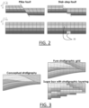
- FIGs. 2-3 illustrate configurations that lead to ambiguous situations.
- FIG. 2 illustrates stair-step faults, by comparing a pillar fault vs a stair-step fault.
- the grid is no more aligned on the faults but is rather torn by them, individual cells maintaining their orthogonality. Consequently, (i) faults do not appear as simple planes in the grid but rather as stair-stepped collections of cell faces, and (ii) cells can be missing near faults creating an apparent ambiguity on the unit thickness - and therefore on all related properties - even in very simple configurations.
- stair-step fault representation creates dead cells 22 around faults. The computation of the stratigraphic thickness in the fault vicinity is easy in the pillar fault case - just counting the number of cells for instance - but tricky in the stair-step fault case.
- FIG. 3 illustrates non-stratigraphic grid layering, by comparing a pure stratigraphic grid vs a sugar box grid.
- stratigraphic organization of the reservoir is complex, explicitly introducing every stratigraphic boundary in the grid might introduce too many degenerated configurations (e.g. pinched cells, and/or highly non-coplanar faces).
- degenerated configurations e.g. pinched cells, and/or highly non-coplanar faces.
- Only a few stratigraphic limits are selected and used to build the grid and control its layering.
- intermediate limits are painted into the grid to complete the stratigraphic column, for example with the painting method.
- the resulting grid is often named sugar box as the stratigraphic units cut the layering. This approach preserves mesh quality, but the generated grid layering does not represent the actual pseudo-geological time.
- a stratigraphic layering derived from the initial grid layering and accounting for all limits and deposition styles, can be computed to provide the grid with stratigraphic information, for example with the layering method.
- stratigraphic information for example with the layering method.
- the pure stratigraphic approach results in a grid with very irregular cells.
- the sugar box approach succeeds in producing very regular cells by not using the stratigraphic limits during the grid construction.
- the grid layering does not reflect the stratigraphy so a layering property may be provided.
- Pillars of the grid are considered.
- a pillar consists of all cells ( i, j, k Grid ) having the same indices i and j , or equivalently a pillar designates a respective i,j couple.
- each cell in addition to its respective grid layering index k Grid , each cell further has a respective stratigraphic layering index k Geol , either defined at the initialization of the pseudo-stratigraphic grid or later, for example by an iteration of the layering method. All indices herein are integers.
- the method comprises providing a surface having a first region and a second region.
- providing a surface it is meant the provision of specifications representing a physical and coherent surface (i.e. a real surface of the environment), such a geological surface (e.g. a horizon).
- the second region is complementary to the first region in the surface. In other words, the union of the first region and of the second region form the surface.
- Each connected part of the second region may be adjacent to at least one connected part of the first region.
- the surface may be provided in the xyz domain rather than in a layering domain of the pseudo-stratigraphic grid.
- locating the surface in the stratigraphic layering domain is not straightforward. Indeed, a direct painting of the surface in the x,y,z domain of the grid would yield to inaccuracy, as it would not account for the approximations performed by the gridding (inherent to its pseudo-stratigraphic nature).
- the method comprises locating the surface in the stratigraphic domain of the grid. For that, the method comprises determining a respective stratigraphic layering value k* Geol ( i,j ) for each pillar i,j intercepted by the surface.
- the stratigraphic layering values can be non-integers.
- the method determines a respective first stratigraphic layering value k* Geol ( i,j ) based on the relative position of the surface in the first pillar.
- the surface intersects the first pillars, and the method makes use of the stratigraphic layering indices of the cells where the surface intersects the pillar.
- the relative position of the surface in the first pillar is deemed to be reliable (in representing stratigraphy), because it is deemed that the first pillar was not impacted during construction of the pseudo-stratigraphic grid.
- the method determines a respective second stratigraphic layering value k* Geol ( i,j ) by interpolating and/or extrapolating first stratigraphic layering values.
- the relative position of the surface in the second pillar (if any) is deemed to be unreliable.
- first stratigraphic layering values are used.
- the method comprises interpolating and/or extrapolating first stratigraphic layering values to output second stratigraphic layering values therewith.
- interpolating and/or extrapolating designates any algorithm that extends coherently the domain of a function, for example iteratively, relying on already-existing values of the function.
- the surface may be provided in the x,y,z domain and the surface intersects the first pillars in said x,y,z domain.
- the surface does not necessarily intersect the second pillars in x,y,z domain.
- the surface may indeed merely intersect the portion of the subsoil represented by at least one second pillar.
- the method may comprise identifying first pillars and second pillars in any manner, based on a geological analysis of the surface. For example, the method may determine a convex hull of a projection of the surface on the x,y domain. The method may then identify the first region as part of the projection, and the second region as the complementary portion in the projection.
- the surface may be a surface which was not used when constructing the pseudo-stratigraphic grid.
- the surface may represent a geological surface detected based on a seismic campaign or a seismic analysis performed after the construction of the pseudo-stratigraphic grid. Or the geological surface may have been set aside at the time of said construction.
- the second region of the surface may present a discontinuity (in the xyz domain).
- the discontinuity may in fact correspond to a continuity in the stratigraphic domain.
- the interpolation and/or extrapolation allows to represent such continuity.
- the discontinuity may be representative of a geological phenomenon making the position of the surface in the grid unreliable for determining stratigraphy.
- the method may comprise determining the first region and the second region.
- the determining may comprise defining a boundary of the second region, and optionally defining the first region as the remainder.
- the boundary may be defined according to a distance criterion relative to the discontinuity.
- the definition may be performed automatically or via user-interaction (manually or semi-automatically).
- the distance criterion may for example involve a cutoff distance e.g.
- the cutoff distance may be higher than 1 or 2 cells and/or lower than 10 or 5 cells. Alternatively or additionally, the distance may be defined via "rough" painting.
- the method may comprise determining automatically a core of the second region, and the user may be offered with the possibility to extend said core. This is illustrated by FIGs. 4-8 .
- the method is applied for inserting horizon 42 into a grid 40.
- the represented situation presents a discrepancy. Indeed, horizon 42 does not follow the top or the base of any geological unit 44 or 46. It is not guaranteed that the grid and the horizon are perfectly coherent (e.g. due to a sampling problem, and/or a simplification of the grid at its creation). Thus, by naively painting the horizon in the grid (i.e. in the xyz domain), cells will not be assigned to the correct region ( FIG. 4).
- FIG. 5 shows that the method allows by extrapolation 52 in the domain ijk to solve these ambiguities.
- the method is applied for inserting horizon 62 into a grid 60.
- a fault 68 there may be a geometrical incoherence between the position of the fault in the grid and the position of the fault in the horizon (e.g. due to a sampling problem, and/or a simplification of the grid at its creation).
- FIG. 7 shows that the method allows by extrapolation 72 in the domain ijk to partly solve these ambiguities (the figure does not show how the bottom left section of the horizon 62 is shortened to handle its crossing the fault 68 in the grid domain).
- pieces of the horizon that are near the fault are part of the second region. They are therefore ignored and interpolated from the first region, that is to say a part of the horizon far from the fault. This amounts to cutting a piece of the horizon.
- the method may detect faulty cells defining the core of the R2 region.
- the user can add criteria to extend this region, for example if the fault is rather horizontal, its influence will be greater and cells may be added (R2 extended).
- R2 extended cells may be added
- R2 convex a last region is created (R2 convex).
- the reservoir may comprise a geological structure which intersects the surface and yields the discontinuity.
- a geological structure moves geological units one relative to another so as to create a discontinuity in the xyz domain in a zone continuous in the stratigraphic domain.
- the geological structure may be a fault or an unconformity.
- the pseudo-stratigraphic grid may represent the fault or unconformity with a stair-step structure. In such a case, correspondence between the xyz and the stratigraphic domain may be particularly an issue.
- the surface may represent a horizon, that is, a surface substantially parallel to the stratigraphy. In such a case, impacts of a mistake in correspondence between the xyz and the stratigraphic domain may be of particular importance.
- the surface may represent a fluid contact (e.g. aquifer surface, or water-gas contact), an intrusive body surface (e.g. salt, shale, volcanic), a diagenetic surface (e.g. karst), a geological body surface - such as a reservoir property boundary surface, a salt diapirism surface, or a channel surface-, or a front surface of a steam presence zone.
- the surface may also be user-defined, for example arbitrarily.
- determining the respective first stratigraphic layering value comprises computing a proportion of the first pillar above the surface.
- the method may perform a Lagrangian interpolation in this respect, when the surface is regularly sampled. In such a case, the Lagrangian interpolation allows to have value of the horizon at any point of space.
- the method may consider the surface to be flat at the scale of the pillar, which allows to make calculations more quickly. The Lagrangian interpolator allows this.
- the method may for each cell calculate the proportion of the cell above the surface. In extreme cases, the proportion is 0 if the cell is fully under the surface and 1 if the cell is fully above the surface.
- the calculation of this proportion may take into account that (1) the cell is not regular and that (2) the surface is in fact a regularly sampled 2D grid, i.e. a map whose value is known at certain points (x, y) regularly distributed.
- One solution for the method is to reshape the cell into tetrahedrons and transform the horizon into a triangulated surface.
- the method may then calculate exactly the intersection between the cell and the surface and then calculate the actual volume of the upper and lower parts of the cell and deduce the proportion. This calculation is nevertheless relatively expensive because the intersections present any form. And in applications it may not be worth working with such a level of precision.
- the method may calculate the depth of the horizon at the midpoint of the pillar.
- a bi-linear interpolation may be used. The calculation is simplified because the method always has four neighbors which, after transformation of the coordinates, define a unit square (see the hyperling https://en.wikipedia.org/wiki/Bilinear_interpolation, ⁇ 1.2.Unit square, at the time of the priority date of the present application).
- the method may further comprise smoothing the first stratigraphic layering values before the interpolation and/or extrapolation.
- Surface e.g. horizons
- the smoothing corrects that.
- Interpolating first stratigraphic layering values may be performed by linear interpolation or gridding.
- the method may create an interpolation mask, meaning the collection of all i,j pillars that will be re-interpolated in the following step.
- the method may do so before cleaning, so as to respect the initial shape and extension of the 2D function.
- the method may compute the points cloud envelop in the i,j domain.
- the mask allows to make an interpolation, but also an extrapolation if needed.
- the method may comprise defining a limit to the extrapolation (e.g. with an envelope). If the surface has a peripheral cavity, the method may fill said cavity.
- the first region may be the footprint of the surface in top view, and the outline of this footprint may be simplified.
- the method may make it a bit convex, and for that the method may apply extrapolations (after envelope extraction).
- the method may extrapolate beyond the second region, and calculate values for a third region to render the surface more convex.
- the method may further interpolate the k Geol in the i,j domain of the reservoir grid using any 2D methods (e.g. gridding) in the predefined mask.
- Gridding is a widely known and complete algorithm. Gridding minimizes the second derivative of the surface (curvature), which provides a good result.
- the gridding algorithm itself may manage the interpolation/extrapolation choice.
- the algorithm used for interpolation/extrapolation may thus be a gridding, also called “convergent interpolation", which is classical in geosciences. This is a multi-resolution method that handles both interpolation and extrapolation. This is algorithm is now discussed, with reference to its implementation in Petrel 2016.3 (registered trademark).
- Convergent interpolation is a control point orientated algorithm (rather than grid point) which will converge upon the solution iteratively adding more and more resolution with each iteration. This means that general trends are retained in areas with little data while detail is honored in areas where the data exists.
- Convergent interpolation is the surface gridding and smoothing algorithm used when building a structural model, creating a single surface model or smoothing a grid. It is a general-purpose algorithm suited to a variety of data types of various densities, some of which are: 3D seismic, 2D seismic, well markers and contour data. It is generalized to handle line-type data (e.g., fault interpretations), dense point data (horizon interpretation grids), sparse point data (horizon marker interpretations), or combinations of these and other data types. It uses methods to honor data approximately (geophysical data) or exactly (geologic data). It uses a fast algorithm which builds the model in stages by iterating or converging from an initial to a final solution.
- FIG. 10 shows an example of how a model is built up this way, exposing results of internal iterations.
- the top surface is the final solution and shows input data as points. Notice the extrapolation characteristics and how its gradient favors the implied data gradient near the data's edge.
- the bottom surface is the initial iteration, which is fitted to the data points.
- Four (4) iterations were performed to build this model, each at a different grid interval. The interval of each iteration is shown as the grid lattice graphic for all but the last (final) iteration. Starting with an initial coarse grid, a factor resolution change of 2 is applied between iterations. Between the last and next to last iterations, an exact factor is applied to achieve the final grid resolution.
- the method may further comprise, for one or more cells of the pseudo-stratigraphic grid (e.g. all cells of the first and second pillars), determining the position of the cell relative to the surface. Such determination is performed based on a comparison of the respective stratigraphic layering index of the cell with the respective first stratigraphic layering value determined for the pillar of the cell if it is a first pillar, or with the respective second stratigraphic layering value determined for the pillar of the cell if it is a second pillar. In such a case, the painting allows to determine how a surface divides cells of the grid.
- the pseudo-stratigraphic grid e.g. all cells of the first and second pillars
- the method may further comprise constructing at least one geological unit based on the determined position of the one or more cells relative to the surface.
- the painted surface may divide an existing geological unit in two subunits, and the method may comprise replacing said existing geological unit by the subunits in the model of the reservoir.
- the painting method allows to integrate in a grid a stratigraphic surface that was not used when creating the grid, for example to cut more finely an existing unit.
- the representation of a surface intersecting the stratigraphy in a grid is not easy if the latter is complex.
- the painting method allows to integrate a new surface into a grid while avoiding the ambiguities of purely geometric methods.
- the painting method proposes to consider that the surface to be introduced into the grid is a function of the parameters ( ij,k Geol ) of the grid.
- the surface initially defined in coordinates ( X,Y,Z ) is transferred geometrically into the grid to be transformed into coordinates ( ij,k Geol ) and ambiguities are handled in this domain.
- the method may determine, for all the cells of the grid, whether they are above or below this surface.
- the surface is considered as a function in the domain of the grid, which facilitates its interpolation.
- the algorithm is fast and robust and solves degenerate cases much more effectively than purely geometric methods.
- the painting method may integrate any surface into an existing grid without having to recalculate the grid. Coupled with the creation of the geological k, the painting method also makes it possible to use this surface in the rest of the geomodelisation workflow.
- the pseudo-stratigraphic grid represents geological units.
- the provided data comprise data associating portions of the grid to geological units, for example cell-to-unit association.
- each geological unit comprises a respective top and a respective base, which are surfaces delimiting vertically the unit.
- Each geological unit also has a respective stratigraphic style (i.e. a manner defining how the stratigraphy is arranged in terms of layering, e.g. represented in any manner in the provided data).
- stratigraphic style i.e. a manner defining how the stratigraphy is arranged in terms of layering, e.g. represented in any manner in the provided data.
- Such geological units may be defined via the painting method, and/or via geological analysis e.g. based on seismic data.
- the layering method comprises performing a local layering scheme for at least one geological unit.
- the at least one geological unit may be a unit not included in the grid.
- the grid is associated to data delimiting the geological unit, as explained above.
- the at least one geological unit may be one for which such data is not present.
- the local layering scheme comprises computing a top 2D map top (.) representing the respective top and a base 2D map base (.) representing the respective base.
- the 2D maps are merely 2D functions associating to a 2D parameter domain, such as i,j,a respective 3D image (e.g. in the z domain or in the k geol domain).
- the local layering scheme comprises defining a gridding constraint depending on the respective stratigraphic style.
- the gridding constraint is any data that indicates how to perform a gridding, and the local layering scheme uses a constraint that is a function of the respective stratigraphic style (so that the gridding is performed according to the respective stratigraphic style).
- the local layering scheme further comprises, for each cell of the respective portion, calculating a respective local stratigraphic layering index dk* Geol based on the top 2D map, on the base 2D map, on the gridding constraint and on the respective stratigraphic style.
- the respective local stratigraphic layering index dk* Geol is an integer.
- the method may comprise computing a non-integer value, and rounding the value to an integer (such a non-integer calculation followed by a rounding is notably performed in the later-discussed examples).
- the stratigraphic layering index is defined for each cell once and for all at the time of constructing the grid.
- the layering method allows to define a new geological unit or subunit (not relied upon when constructing the grid), and to compute a new value for the stratigraphic layering index that replaces the old value.
- Invention Examples of the layering method are now discussed.
- the at least one geological unit may comprise several geological units that form the reservoir.
- the local layering scheme may be performed for several distinct (e.g. and non-overlapping) units.
- the method may further comprise determining, for each cell of the pseudo-stratigraphic grid, a respective global stratigraphic layering index based on the respective local stratigraphic layering index and on a global recombination scheme. This allows obtaining stratigraphic layering indices globally consistent across units.
- the global recombination scheme is any scheme based on information indicating stratigraphy between the several units, and that transforms the local indices into global indices in a manner consistent with the stratigraphy between the several units and with the stratigraphy within each unit (provided by the local indices).
- local indices it is merely meant the indices outputted by the method based solely on the top 2D map, on the base 2D map, on the gridding constraint and on the respective stratigraphic style, and thus before any global recombination scheme.
- global indices, it is merely meant the transforms thereof determined by the global recombination scheme.
- the layering method may be performed with a grid already provided with stratigraphic layering indices.
- the method may comprise providing, for each cell of the respective portion, a respective initial stratigraphic layering index k Geo / .
- initial it is merely meant “already associated to the grid”.
- the method may comprise replacing the respective initial stratigraphic layering index.
- the replacement indices may be the local indices or the global indices (if any), depending on the situation.
- the top (resp. base) has a first region and a second region complementary to the first region.
- the top (resp. base) 2D map outputs, for each cell of the top (resp. base), a respective local stratigraphic value.
- the computing of the top (resp. base) 2D map includes, for each first cell of the first region, determining a respective first stratigraphic layering index k* Geol ( i,j ) based on the respective initial stratigraphic layering index, and, for each second pillar i,j intercepted by the second region, determining a respective second stratigraphic layering value k* Geol ( i,j ) by interpolating first stratigraphic layering values.
- the layering method here performs an interpolation in the manner of the painting method, to improve robustness and accuracy at regions of the top (resp. base) for which the values of the 2D map are unreliable.
- the interpolation may be performed as described with respect to the painting method. Unlike the painting method, the layering method may limit such correction to interpolations, that is, with no extrapolation at all (e.g. and thus no abovementioned "third" region). Furthermore, the interpolation may be performed without user-intervention, and be limited to the earlier-mentioned core region.
- the first stratigraphic layering indices may be said initial stratigraphic layering indices. In case no stratigraphic layering index is available at all, the first stratigraphic layering indices may be the gridding indices.
- FIGs. 11-12 show examples of two anomalous cases and how such interpolation can correct them. It is considered that the method is applied for determining a new layering in the non-colored geological unit, of which top is not of constant depth and layer number, and is bordered by a fault on its side.
- the method may for example consider an iso-proportional layering.
- the figure shows example values for dt (see later).
- the result is not correct under the fault. Indeed, without the interpolation, the algorithm considers that the fault is the top of the unit.
- the method re-interpolates the top of the unit and calculates the dt with respect to this interpolated top. The result is correct.
- the method may for example consider a follow-top layering.
- the figure shows the schematic dk Geol ⁇ .
- the result is not correct under the fault. Indeed, without the interpolation, the algorithm considers that the fault is the top of the unit.
- the method re-interpolates the top of the unit and calculate the dt with respect to this interpolated top. The result is correct.
- the second region may be present a discontinuity.
- the reservoir may for example comprising a geological structure which intersects the surface and yields the discontinuity.
- the geological structure is a fault or an unconformity.
- the method may comprise detecting such faulted cells of the top (resp. base) based on topology of the pseudo-stratigraphic grid.
- FIGs. 13-14 show two configurations among others presenting a lateral disconnection between two cells. Note that only one non-shared point is enough to create a disconnect.
- the respective stratigraphic style may be a true iso-proportional style. Indeed, this case is related to the number of cells in a pillar and so yielding a number of precise layers (the same everywhere) is of particular importance. Also, the computations may require (as discussed later) both the top and bottom. In such a case, the method may use k geo / (while it may use z in other cases as it may be sufficient). Using k geol in the a true iso-proportional style case leads to accuracy. In other styles, using z is sufficient, so there may be no need for a k geo / and its interpolation.
- the top 2D map and/or the base 2D map each output, for each pillar i,j intercepting the at least one geological unit, a respective value top ( i,j ) or base ( i,j ) of a vertical positioning measure, which may be k Geol (.), or the value z (.) (e.g. in which case the value for the cell barycenter may be used).
- the calculating may include establishing a respective pseudo relative depositional time dt, based on a comparison between a respective value of the vertical positioning measure at the cell and the respective value outputted by the first and/or base 2D map.
- the calculating may further include converting the respective pseudo relative depositional time into the respective local stratigraphic layering index based on the gridding constraint and/or a comparison between the top 2D map and the base 2D map.
- the establishing and the converting may be performed further based on the respective stratigraphic style. This provides efficiency to the method.
- the gridding constraint may be a target number of cells, and the converting may include multiplying the target number of cells with the respective pseudo relative depositional time.
- the gridding constraint may be a target cell thickness
- the converting may include multiplying a max of the difference between the top 2D map and the base 2D map with the respective pseudo relative depositional time, divided by the target cell thickness. This leads efficiently to accurate results.
- the following discusses examples of establishing a respective pseudo relative depositional time based on the respective stratigraphic style.
- dt is 1 on the top, 0 on the base and 0.5 in the middle.
- the repository chosen may be the initial layering or the true depth. This choice of repository may be left to the user according to the following choices:
- the vertical thickness of the cells is fixed, but because the thickness of the unit varies horizontally, the number of cells is not known and varies in space. Since it is the thickness that is fixed, the method may work in the depth domain rather than in the field of initial layering.
- n min 1 t max t
- t is the target cell thickness entered by the user.
- dt is 0 at the top of the horizon and is 1 at the base where the unit is the thickest.
- dt is 0 at the base of the horizon and is 1 at the top where the unit is the thickest.
- dk Geol * dt ⁇ n ⁇ [ 0 , n ⁇ 1 [
- the layering method thus allows to generate a geological layering property directly in the reservoir grid, respecting stratigraphic constraints within units.
- the calculation of the geological k is done directly in the reservoir grid respecting stratigraphic constraints within units (which may be conformal, erosive or deposited on a paleotopography).
- the filling can then be done using this geological k instead of using the k of the grid as is conventionally done. This avoids grid distortion problems and simplifies the construction of the grid.
- the calculation of this property is done directly in a "sugar box" grid using stratigraphic constraints.
- the resulting grid is directly usable for geostatistical and dynamic simulations, without cell distortion, while maintaining a correct definition of the stratigraphy.
- the creation of this property does not require complex structural modeling and the creation of a grid consistent with the stratigraphy. It is made directly in a simple grid. The simulation methods may then use this stratigraphic property in place of the grid layering.
- the example implementation may thus consist of a method of integrating a new horizon into a pseudo-stratigraphic reservoir grid.
- the method may include the following steps:
- the method ultimately allows to obtain new geological units.
- the example implementation may thus consist of a layering method in a pseudo-stratigraphic reservoir grid.
- the method may include the following steps:
- the example implementation ultimately allows a layering that avoids problems of grid distortion which simplifies the construction of the grid.
- the example application was based on handling a pseudo-stratigraphic approach. It was decided for flow simulation accuracy to limit as much as possible the pinches between the units, thus to use only the top and base of the reservoirs (B225 and B275) to build the grid. Intermediate interpretations, bounding erosive subunits inside the reservoir, were not used directly for the grid generation but only afterwards, in a pseudo-sugar box approach. Also, some of the unit boundaries were not interpreted on the seismic, but were defined inside a unit using proportional layers (C7 - L1 to L3).
- This approach required to paint the units into the grid, to compute a geological layering inside the painted units, in order to get a stratigraphic continuity of the layering to perform geostatistics simulations. This new layering is also required to subdivide unit C7.
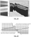
- FIG. 18 shows the stratigraphy of a hydrocarbon field.
- B225 and B275 are the two horizons used for building the reservoir grid;
- M5 base is a regional erosive surface,
- C5 base is a locally erosive surface.
- C6 and C7 are conformable units that are eroded by both C5 and M5.
- the classical approach which performs a vertical projection of the raw horizon surface, generates holes in the vicinity of faults. Holes are related both to small discrepancy between input horizon surface - often interpreted on the seismic and therefore controlled by seismic faults - and stair-step faults, but also to missing cells along stair-step faults.
- FIG. 19 shows such direct horizon painting. Geometric ambiguities appear when painting a faulted horizon near a stair-step fault.
- FIG. 20 further shows direct painting of the horizons in the grid using a horizon filter module.
- the resulting property is affected by holes (arrows). These artifacts can affect a large part of the grid and can be tedious to analyze and QC. To correct this effect, it was proposed to use the painting method in the following way: 1) filter around the faults and 2) re-interpolate the painted property in order to 3) get a properly painted unit property.
- the painting method cleans the painted property using a given filter, and re-interpolates this property in the cleaned area.
- the interpolation is performed in the stratigraphic domain to ensure valid output unit. All these properties - one per horizon - may be combined to generate units.
- the filter can be defined from any condition or combination of conditions.
- the areas that cause issues when painting a horizon into a grid are along the stair step faults. Consequently, the filter may be a cutoff on the distance to faults. For this reason, a fault region is created, collecting all the cells that are intersected by the faults - it is possible to compute directly the distance to the fault surfaces using a multi-condition filter, but it is tedious and not recommended.
- FIG. 21 shows fault region creation. Faults are selected to build a region in the grid. Resulting region is displayed on the right.
- the resulting region may then be used as a seed to compute the distance to the faults, in number of cells. It should be noted that because the filtering region is versatile, tailor made conditions can be designed, for instance to adapt the filtering to different fault families.
- FIG. 22 shows distance to fault computation. A distance to fault property (expressed in number of cells) was thus computed.
- a Smart horizon painting module can then be applied to compute a property per horizon in the grid; this property equals -1 above the horizon and +1 below (see FIG. 23 ).
- This process may be applied for all the horizons bounding the units; it then generates four properties.
- FIG. 23 shows smart horizon painting. Horizons painting using the new dedicated module, with an interpolation of the generated properties. Paint results for of every interpreted horizons M5 base, C5 base, C6 base and C7 base show neither holes nor artifacts.
- Another module can be applied to combine the created properties and generate a unit property. This is a series of logical operations based on a given stratigraphic column. The properties corresponding to the horizons are given in a specific order, a unit being defined between two horizons and corresponding to a unique value. By default, the unit property increases from top to bottom and starts at 1, but this can be edited.
- the layering of the grid (corresponding to the k index of the cells) was built as an isoproportional layering between the top and the base without accounting for the internal stratigraphy; it has no stratigraphic meaning. It is thus mandatory for property modeling to compute a stratigraphic layering based on the newly created unit property.
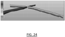
- FIG. 24 shows the grid layering generated using an isoproportional layering between B225 and B275, the top and base of the reservoir grid. This layering does not reflect the stratigraphic continuities.
- a new layering was computed using a module "Create geological layering". This module allows, like classical structural modeling, to define the layering in each of the units, associated with a number of cells if isoproportional layering is chosen, and a cell thickness if a follow top or base layering is selected.
- FIG. 25 shows the new layering computation using the module Create geological layering, respecting the stratigraphic relationships of the column.
- unit C7 was equally divided into three subunits C7 L1, L2 and L3, and the last one, L3, was divided into an upper and a lower part, corresponding respectively to 1/3 and 2/3 of C7 L3 thickness ( FIG. 26 ).
- FIG. 26 shows subunits definition in C7, using the newly created stratigraphic layering for dividing equally the three layers, and then dividing L3 layer into 2/3 and 1/3 respectively for the upper and lower parts. This is done using a filter on the stratigraphic layering property in Create/Modify property.
- the Fit grid to wells module may account for a geological layering.
- the subunits that are defined are respected and the reservoir grid can be fitted to associated markers.
- a multi-condition filter allowed working with the units defined by the Smart unit painting, or with the stratigraphic layering. For instance, for a more efficient check of the facies and petrophysical properties simulated using the geological layering, one may use the filter to visualize the results of the simulation in each geological layer, instead of doing this in each grid layer (see FIG. 27 ). To perform the QC of the grid generation and unit painting, it is possible to compute the residuals using a filter on the unit property. This property can also be used directly to extract top and base horizons of the units.
- HuPhiSo maps computation modules also offer the possibility to use a multi-condition filter, allowing using the stratigraphic layering instead of the grid layering.
- FIG. 27 shows the grid layering visualization vs. Stratigraphic layering visualization.
- the grid K visualization does not show the stratigraphic continuities as it crosses several units.
- the stratigraphic layer visualization applied with a multicondition filter, allows to properly check the geostatistical simulations.
- the new workflow allows combining a complex stratigraphy with grid quality constraints needed for dynamic simulations, by dissociating the grid geometry from the true geometry of the reservoir.
- Grids that follow this principle are named pseudo-stratigraphic because the cell k index is not related anymore to its stratigraphic location.
Landscapes
- Physics & Mathematics (AREA)
- Life Sciences & Earth Sciences (AREA)
- General Life Sciences & Earth Sciences (AREA)
- General Physics & Mathematics (AREA)
- Geophysics (AREA)
- Geophysics And Detection Of Objects (AREA)
Claims (11)
- Procédé mis en oeuvre par ordinateur de géomodélisation, le procédé comprenant :- la fourniture d'une grille pseudo-stratigraphique, où la grille pseudo-stratigraphique est obtenue sur la base d'un ensemble de référence de structures géologiques, et où les structures géologiques sont définies sur la base d'une analyse géologique de données géologiques ou géophysiques qui comprennent des données sismiques acquises par un ou plusieurs capteurs sismiques et/ou pendant un ou plusieurs relevés sismiques du réservoir, la grille pseudo-stratigraphique représentant un réservoir comportant des unités géologiques, la grille pseudo-stratigraphique comportant des piliers (i,j), chaque pilier comprenant des cellules respectives (i,j,k), chaque unité géologique étant représentée par une partie respective de la grille pseudo-stratigraphique et ayant un sommet, une base et un style stratigraphique respectifs ; puis- pour au moins une unité géologique :le procédé comprenant en outre :o le calcul d'une carte 2D de sommet (top(.)) représentant le sommet respectif et une carte 2D de base (base(.)) représentant la base respective ;o la définition d'une contrainte de maillage (n,t) suivant le style stratigraphique respectif ;o pour chaque cellule de la partie respective, le calcul d'un indice de stratification stratigraphique local respectif (dk* Geo/) sur la base de la carte 2D de sommet, de la carte 2D de base, de la contrainte de maillage et du style stratigraphique respectif ; eto la configuration de la grille pseudo-stratigraphique pour une simulation géologique, par ajout aux données de grille représentatives d'informations de stratification relatives à l'unité géologique respective ;et où la simulation géologique délivre en sortie au moins l'un parmi la pression de champ moyenne en fonction du temps ; les profils de production cumulée totale de champ de pétrole, d'eau et de gaz au cours du temps ; les taux de production de champ total journaliers, hebdomadaires, mensuels ou annuels de chaque phase : pétrole, eau et gaz ; les pressions de puits individuels au cours du temps ; les débits de puits individuels cumulés et journaliers de pétrole, d'eau et de gaz au cours du temps ; des teneurs en eau de champ total ou de puits individuels, les rapports gaz/pétrole, GOR, les rapports pétrole/eau, O/W au cours du temps ; et/ou la répartition spatiale des saturations en pétrole, en eau et en gaz dans l'ensemble du réservoir en fonction du temps ;- la fourniture, pour chaque cellule de la partie respective, d'un indice de stratification stratigraphique initial respectif (kGeol ) ; et- le remplacement de l'indice de stratification stratigraphique initial respectif ; caractérisé en ce que :- le sommet et/ou la base comporte une première région et une deuxième région complémentaire de la première région,- la carte 2D de sommet et/ou de base délivre en sortie, pour chaque cellule du sommet et/ou la base, une valeur stratigraphique respective locale (top(i,j), base(i,j), et- le calcul de la carte 2D de sommet et/ou de base comprend :o pour chaque première cellule de la première région, la détermination d'un premier indice de stratification stratigraphique respectif (k*Geol(i,j)) sur la base de l'indice de stratification stratigraphique initial respectif ; eto pour chaque deuxième pilier (i,j) intercepté par la deuxième région, la détermination d'une deuxième valeur de stratification stratigraphique respective (k*Geol(i,j)) par interpolation de premières valeurs de stratification stratigraphique.
- Procédé selon la revendication 1, dans lequel l'au moins une unité géologique comprend plusieurs unités géologiques qui forment le réservoir, le procédé comprenant en outre la détermination, pour chaque cellule de la grille pseudo-stratigraphique, d'un indice de stratification stratigraphique global respectif sur la base de l'indice de stratification stratigraphique local respectif et d'un schéma de recombinaison global.
- Procédé selon la revendication 1 ou la revendication 2, dans lequel la deuxième région présente une discontinuité, le réservoir comprenant éventuellement une structure géologique qui coupe la surface et produit la discontinuité.
- Procédé selon la revendication 3, dans lequel la structure géologique est une faille ou une discordance.
- Procédé selon la revendication 4, le procédé comprenant la détection de cellules faillées du sommet ou the base sur la base de la topologie de la grille pseudo-stratigraphique.
- Procédé selon l'une quelconque des revendications 1 à 5, dans lequel le style stratigraphique respectif est un style iso-proportionnel vrai.
- Procédé selon l'une quelconque des revendications 1 à 6, dans lequel la carte 2D de sommet et/ou la carte 2D de base délivrent chacune, pour chaque pilier (i,j), l'interception de l'au moins une unité géologique, une valeur respective (top(i,j), base(i,j)) d'une mesure de positionnement vertical (kGeol (.),z(.)), le calcul comprenant :- l'établissement d'un temps de dépôt pseudo-relatif respectif sur la base d'une comparaison entre une valeur respective de la mesure de positionnement vertical au niveau de la cellule et la valeur respective délivrée par la carte 2D de sommet et/ou de base ; et- la conversion du temps de dépôt pseudo-relatif respectif en indice de stratification stratigraphique local respectif sur la base de la contrainte de maillage et/ou d'une comparaison entre la carte 2D de sommet et la carte 2D de base ;l'établissement et la conversion étant effectués en outre sur la base du style stratigraphique respectif.
- Procédé selon la revendication 7, dans lequel le style stratigraphique respectif est un style iso-proportionnel vrai ou un style iso-proportionnel avec option géométrique, et/ou la contrainte de maillage est un nombre de cellules cible, la conversion comprenant la multiplication du nombre de cellules cible par le temps de dépôt pseudo-relatif respectif.
- Procédé selon la revendication 7 ou 8, dans lequel le style stratigraphique respectif est un style follow-top (suivre le sommet) ou un style follow-base (suivre la base), et/ou la contrainte de maillage est une épaisseur de cellule cible, la conversion comprenant la multiplication d'un maximum de la différence entre la carte 2D de sommet et la carte 2D de base par le temps de dépôt pseudo-relatif respectif, divisé par l'épaisseur de cellule cible.
- Programme informatique comprenant des instructions pour conduire le procédé selon l'une quelconque des revendications 1 à 9.
- Système comprenant un processeur couplé à une mémoire, la mémoire comportant, enregistré sur celle-ci, le programme informatique selon la revendication 10.
Applications Claiming Priority (1)
| Application Number | Priority Date | Filing Date | Title |
|---|---|---|---|
| PCT/IB2020/000071 WO2021148830A1 (fr) | 2020-01-22 | 2020-01-22 | Structuration en couches pour la géomodélisation |
Publications (2)
| Publication Number | Publication Date |
|---|---|
| EP4073554A1 EP4073554A1 (fr) | 2022-10-19 |
| EP4073554B1 true EP4073554B1 (fr) | 2024-04-24 |
Family
ID=70057161
Family Applications (1)
| Application Number | Title | Priority Date | Filing Date |
|---|---|---|---|
| EP20715443.6A Active EP4073554B1 (fr) | 2020-01-22 | 2020-01-22 | Stratification pour la géomodélisation |
Country Status (3)
| Country | Link |
|---|---|
| US (1) | US12596203B2 (fr) |
| EP (1) | EP4073554B1 (fr) |
| WO (1) | WO2021148830A1 (fr) |
Families Citing this family (4)
| Publication number | Priority date | Publication date | Assignee | Title |
|---|---|---|---|---|
| CN119105079B (zh) * | 2023-06-08 | 2026-04-07 | 中国石油天然气集团有限公司 | 一种井震结合建立高精度地层模型剖面的方法 |
| CN117826257B (zh) * | 2023-12-28 | 2024-06-11 | 西南石油大学 | 一种油气二次运移通道的三维表征方法 |
| CN119149653B (zh) * | 2024-07-31 | 2025-04-04 | 中国地质调查局发展研究中心 | 地质体的描述方法、装置和电子设备 |
| CN119399394B (zh) * | 2024-11-11 | 2025-12-02 | 四川省地质大数据中心 | 一种基于ai的无属性地质图建库方法及系统 |
Family Cites Families (22)
| Publication number | Priority date | Publication date | Assignee | Title |
|---|---|---|---|---|
| US4821164A (en) | 1986-07-25 | 1989-04-11 | Stratamodel, Inc. | Process for three-dimensional mathematical modeling of underground geologic volumes |
| DE60201831D1 (de) | 2002-08-26 | 2004-12-09 | Total Sa | Verfahren zur Berechnung von Maschenmodellen eines Reservoirs |
| US7706981B2 (en) * | 2007-02-08 | 2010-04-27 | Chevron U.S.A. Inc. | Method for generating reservoir models utilizing synthetic stratigraphic columns |
| EP2317348B1 (fr) | 2009-10-30 | 2014-05-21 | Services Pétroliers Schlumberger | Procédé de construction d'un espace sédimentaire correspondant à un domaine géologique |
| EP2499567A4 (fr) * | 2009-11-12 | 2017-09-06 | Exxonmobil Upstream Research Company | Procédé et appareil de modélisation et de simulation de réservoirs |
| US8274859B2 (en) | 2010-02-22 | 2012-09-25 | Landmark Graphics Corporation | Systems and methods for modeling 3D geological structures |
| US20120022837A1 (en) * | 2010-05-18 | 2012-01-26 | Schlumberger Technology Corporation | Smoothing Of Stair-Stepped Geometry In Grids |
| US20110310101A1 (en) * | 2010-06-22 | 2011-12-22 | Schlumberger Technology Corporation | Pillar grid conversion |
| US8965745B2 (en) * | 2011-04-14 | 2015-02-24 | Schlumberger Technology Corporation | Grid from depositional space |
| FR2987138A1 (fr) * | 2012-02-22 | 2013-08-23 | Schlumberger Technology Corp | Titre non renseigne. |
| FR2987903B1 (fr) | 2012-03-09 | 2014-05-09 | Schlumberger Services Petrol | Structures de failles geologiques contenant des non-conformites. |
| US9759826B2 (en) | 2012-04-03 | 2017-09-12 | Paradigm Sciences Ltd. | System and method for generating an implicit model of geological horizons |
| US9182511B2 (en) | 2012-11-04 | 2015-11-10 | Drilling Info, Inc. | System and method for reproducibly extracting consistent horizons from seismic images |
| US20140136171A1 (en) | 2012-11-13 | 2014-05-15 | Chevron U.S.A. Inc. | Unstructured Grids For Modeling Reservoirs |
| GB2512372B (en) | 2013-03-28 | 2020-07-29 | Total Sa | Method of modelling a subsurface volume |
| FR3009415B1 (fr) | 2013-07-31 | 2018-10-26 | Total Sa | Procede d'adaptation d'une representation geologique d'un sous-sol |
| EP2869096B1 (fr) | 2013-10-29 | 2019-12-04 | Emerson Paradigm Holding LLC | Systèmes et procédés de maillage multi-échelle pour modélisation de temps géologique |
| US10571601B2 (en) | 2014-10-09 | 2020-02-25 | Schlumberger Technology Corporation | Geologic fault representation for flow simulation |
| FR3036210B1 (fr) | 2015-05-12 | 2018-07-06 | Services Petroliers Schlumberger | Stratigraphie geologique par fonctions implicites et a saut |
| US9690002B2 (en) | 2015-06-18 | 2017-06-27 | Paradigm Sciences Ltd. | Device, system and method for geological-time refinement |
| US10838108B2 (en) | 2016-12-29 | 2020-11-17 | Exxonmobil Upstream Research Company | Method and system for interpolating discontinuous functions in a subsurface model |
| WO2021148832A1 (fr) | 2020-01-22 | 2021-07-29 | Total Se | Peinture pour géomodélisation |
-
2020
- 2020-01-22 US US17/758,557 patent/US12596203B2/en active Active
- 2020-01-22 WO PCT/IB2020/000071 patent/WO2021148830A1/fr not_active Ceased
- 2020-01-22 EP EP20715443.6A patent/EP4073554B1/fr active Active
Also Published As
| Publication number | Publication date |
|---|---|
| WO2021148830A1 (fr) | 2021-07-29 |
| US12596203B2 (en) | 2026-04-07 |
| US20230043782A1 (en) | 2023-02-09 |
| EP4073554A1 (fr) | 2022-10-19 |
Similar Documents
| Publication | Publication Date | Title |
|---|---|---|
| USRE49507E1 (en) | Faulted geological structures having unconformities | |
| US9600608B2 (en) | Method of constructing a geological model comprising setting a depositional position of stratigraphic units | |
| CA2920499C (fr) | Fonction stratigraphique | |
| EP4073554B1 (fr) | Stratification pour la géomodélisation | |
| US11209560B2 (en) | Assignment of systems tracts | |
| EP3371629B1 (fr) | Présentation d'incertitude structurale dans un maillage représentant un environnement géologique | |
| CN102754105B (zh) | 用于创建历史匹配模拟模型的方法和系统 | |
| US7292241B2 (en) | Process for calculating meshed realizations of a reservoir | |
| EP4073555B1 (fr) | Peinture pour géomodélisation | |
| Lønøy et al. | Geocellular rendering of cave surveys in paleokarst reservoir models | |
| EP3371627B1 (fr) | Attributs sismiques tridimensionnels stratigraphiquement cohérents | |
| US12619000B2 (en) | Painting for geomodeling | |
| EP3918381B1 (fr) | Simulation d'écoulement d'hydrocarbures | |
| Irving et al. | Optimization of uncertain structural parameters with production and observation well data | |
| Hou et al. | Refined Integration of Multilayer DEM-GTP-TEN for Three-Dimensional Quaternary Geological Modeling: A Case Study in Nantong City, China | |
| Thomason et al. | Model creation using stacked surfaces | |
| Aguilar et al. | Handling Complex Stratigraphic Relationships Using Volume Based Modeling and Stair-Step Grids | |
| WO2025065864A1 (fr) | Procédé et appareil de construction d'un modèle de paramètre géophysique direct, et dispositif et support | |
| CN120782982A (zh) | 一种融合地层约束规则的地质体隐式建模方法及系统 | |
| Viseur | Surface-Based 3D Modeling of Geological Structures | |
| Whaley et al. | The Next Generation Subsurface Modelling |
Legal Events
| Date | Code | Title | Description |
|---|---|---|---|
| STAA | Information on the status of an ep patent application or granted ep patent |
Free format text: STATUS: UNKNOWN |
|
| STAA | Information on the status of an ep patent application or granted ep patent |
Free format text: STATUS: THE INTERNATIONAL PUBLICATION HAS BEEN MADE |
|
| PUAI | Public reference made under article 153(3) epc to a published international application that has entered the european phase |
Free format text: ORIGINAL CODE: 0009012 |
|
| STAA | Information on the status of an ep patent application or granted ep patent |
Free format text: STATUS: REQUEST FOR EXAMINATION WAS MADE |
|
| 17P | Request for examination filed |
Effective date: 20220713 |
|
| AK | Designated contracting states |
Kind code of ref document: A1 Designated state(s): AL AT BE BG CH CY CZ DE DK EE ES FI FR GB GR HR HU IE IS IT LI LT LU LV MC MK MT NL NO PL PT RO RS SE SI SK SM TR |
|
| DAV | Request for validation of the european patent (deleted) | ||
| DAX | Request for extension of the european patent (deleted) | ||
| GRAP | Despatch of communication of intention to grant a patent |
Free format text: ORIGINAL CODE: EPIDOSNIGR1 |
|
| STAA | Information on the status of an ep patent application or granted ep patent |
Free format text: STATUS: GRANT OF PATENT IS INTENDED |
|
| INTG | Intention to grant announced |
Effective date: 20231128 |
|
| P01 | Opt-out of the competence of the unified patent court (upc) registered |
Effective date: 20240124 |
|
| GRAS | Grant fee paid |
Free format text: ORIGINAL CODE: EPIDOSNIGR3 |
|
| GRAA | (expected) grant |
Free format text: ORIGINAL CODE: 0009210 |
|
| STAA | Information on the status of an ep patent application or granted ep patent |
Free format text: STATUS: THE PATENT HAS BEEN GRANTED |
|
| AK | Designated contracting states |
Kind code of ref document: B1 Designated state(s): AL AT BE BG CH CY CZ DE DK EE ES FI FR GB GR HR HU IE IS IT LI LT LU LV MC MK MT NL NO PL PT RO RS SE SI SK SM TR |
|
| REG | Reference to a national code |
Ref country code: GB Ref legal event code: FG4D |
|
| REG | Reference to a national code |
Ref country code: CH Ref legal event code: EP |
|
| REG | Reference to a national code |
Ref country code: DE Ref legal event code: R096 Ref document number: 602020029546 Country of ref document: DE |
|
| REG | Reference to a national code |
Ref country code: IE Ref legal event code: FG4D |
|
| REG | Reference to a national code |
Ref country code: NL Ref legal event code: FP |
|
| REG | Reference to a national code |
Ref country code: LT Ref legal event code: MG9D |
|
| REG | Reference to a national code |
Ref country code: AT Ref legal event code: MK05 Ref document number: 1680183 Country of ref document: AT Kind code of ref document: T Effective date: 20240424 |
|
| PG25 | Lapsed in a contracting state [announced via postgrant information from national office to epo] |
Ref country code: IS Free format text: LAPSE BECAUSE OF FAILURE TO SUBMIT A TRANSLATION OF THE DESCRIPTION OR TO PAY THE FEE WITHIN THE PRESCRIBED TIME-LIMIT Effective date: 20240824 |
|
| PG25 | Lapsed in a contracting state [announced via postgrant information from national office to epo] |
Ref country code: BG Free format text: LAPSE BECAUSE OF FAILURE TO SUBMIT A TRANSLATION OF THE DESCRIPTION OR TO PAY THE FEE WITHIN THE PRESCRIBED TIME-LIMIT Effective date: 20240424 |
|
| PG25 | Lapsed in a contracting state [announced via postgrant information from national office to epo] |
Ref country code: FI Free format text: LAPSE BECAUSE OF FAILURE TO SUBMIT A TRANSLATION OF THE DESCRIPTION OR TO PAY THE FEE WITHIN THE PRESCRIBED TIME-LIMIT Effective date: 20240424 Ref country code: HR Free format text: LAPSE BECAUSE OF FAILURE TO SUBMIT A TRANSLATION OF THE DESCRIPTION OR TO PAY THE FEE WITHIN THE PRESCRIBED TIME-LIMIT Effective date: 20240424 |
|
| PG25 | Lapsed in a contracting state [announced via postgrant information from national office to epo] |
Ref country code: GR Free format text: LAPSE BECAUSE OF FAILURE TO SUBMIT A TRANSLATION OF THE DESCRIPTION OR TO PAY THE FEE WITHIN THE PRESCRIBED TIME-LIMIT Effective date: 20240725 |
|
| PG25 | Lapsed in a contracting state [announced via postgrant information from national office to epo] |
Ref country code: PT Free format text: LAPSE BECAUSE OF FAILURE TO SUBMIT A TRANSLATION OF THE DESCRIPTION OR TO PAY THE FEE WITHIN THE PRESCRIBED TIME-LIMIT Effective date: 20240826 |
|
| PG25 | Lapsed in a contracting state [announced via postgrant information from national office to epo] |
Ref country code: ES Free format text: LAPSE BECAUSE OF FAILURE TO SUBMIT A TRANSLATION OF THE DESCRIPTION OR TO PAY THE FEE WITHIN THE PRESCRIBED TIME-LIMIT Effective date: 20240424 |
|
| PG25 | Lapsed in a contracting state [announced via postgrant information from national office to epo] |
Ref country code: AT Free format text: LAPSE BECAUSE OF FAILURE TO SUBMIT A TRANSLATION OF THE DESCRIPTION OR TO PAY THE FEE WITHIN THE PRESCRIBED TIME-LIMIT Effective date: 20240424 |
|
| PG25 | Lapsed in a contracting state [announced via postgrant information from national office to epo] |
Ref country code: PL Free format text: LAPSE BECAUSE OF FAILURE TO SUBMIT A TRANSLATION OF THE DESCRIPTION OR TO PAY THE FEE WITHIN THE PRESCRIBED TIME-LIMIT Effective date: 20240424 |
|
| PG25 | Lapsed in a contracting state [announced via postgrant information from national office to epo] |
Ref country code: LV Free format text: LAPSE BECAUSE OF FAILURE TO SUBMIT A TRANSLATION OF THE DESCRIPTION OR TO PAY THE FEE WITHIN THE PRESCRIBED TIME-LIMIT Effective date: 20240424 |
|
| PG25 | Lapsed in a contracting state [announced via postgrant information from national office to epo] |
Ref country code: PT Free format text: LAPSE BECAUSE OF FAILURE TO SUBMIT A TRANSLATION OF THE DESCRIPTION OR TO PAY THE FEE WITHIN THE PRESCRIBED TIME-LIMIT Effective date: 20240826 Ref country code: PL Free format text: LAPSE BECAUSE OF FAILURE TO SUBMIT A TRANSLATION OF THE DESCRIPTION OR TO PAY THE FEE WITHIN THE PRESCRIBED TIME-LIMIT Effective date: 20240424 Ref country code: LV Free format text: LAPSE BECAUSE OF FAILURE TO SUBMIT A TRANSLATION OF THE DESCRIPTION OR TO PAY THE FEE WITHIN THE PRESCRIBED TIME-LIMIT Effective date: 20240424 Ref country code: IS Free format text: LAPSE BECAUSE OF FAILURE TO SUBMIT A TRANSLATION OF THE DESCRIPTION OR TO PAY THE FEE WITHIN THE PRESCRIBED TIME-LIMIT Effective date: 20240824 Ref country code: HR Free format text: LAPSE BECAUSE OF FAILURE TO SUBMIT A TRANSLATION OF THE DESCRIPTION OR TO PAY THE FEE WITHIN THE PRESCRIBED TIME-LIMIT Effective date: 20240424 Ref country code: GR Free format text: LAPSE BECAUSE OF FAILURE TO SUBMIT A TRANSLATION OF THE DESCRIPTION OR TO PAY THE FEE WITHIN THE PRESCRIBED TIME-LIMIT Effective date: 20240725 Ref country code: FI Free format text: LAPSE BECAUSE OF FAILURE TO SUBMIT A TRANSLATION OF THE DESCRIPTION OR TO PAY THE FEE WITHIN THE PRESCRIBED TIME-LIMIT Effective date: 20240424 Ref country code: ES Free format text: LAPSE BECAUSE OF FAILURE TO SUBMIT A TRANSLATION OF THE DESCRIPTION OR TO PAY THE FEE WITHIN THE PRESCRIBED TIME-LIMIT Effective date: 20240424 Ref country code: BG Free format text: LAPSE BECAUSE OF FAILURE TO SUBMIT A TRANSLATION OF THE DESCRIPTION OR TO PAY THE FEE WITHIN THE PRESCRIBED TIME-LIMIT Effective date: 20240424 Ref country code: AT Free format text: LAPSE BECAUSE OF FAILURE TO SUBMIT A TRANSLATION OF THE DESCRIPTION OR TO PAY THE FEE WITHIN THE PRESCRIBED TIME-LIMIT Effective date: 20240424 Ref country code: RS Free format text: LAPSE BECAUSE OF FAILURE TO SUBMIT A TRANSLATION OF THE DESCRIPTION OR TO PAY THE FEE WITHIN THE PRESCRIBED TIME-LIMIT Effective date: 20240724 |
|
| PG25 | Lapsed in a contracting state [announced via postgrant information from national office to epo] |
Ref country code: DK Free format text: LAPSE BECAUSE OF FAILURE TO SUBMIT A TRANSLATION OF THE DESCRIPTION OR TO PAY THE FEE WITHIN THE PRESCRIBED TIME-LIMIT Effective date: 20240424 |
|
| PG25 | Lapsed in a contracting state [announced via postgrant information from national office to epo] |
Ref country code: EE Free format text: LAPSE BECAUSE OF FAILURE TO SUBMIT A TRANSLATION OF THE DESCRIPTION OR TO PAY THE FEE WITHIN THE PRESCRIBED TIME-LIMIT Effective date: 20240424 |
|
| PG25 | Lapsed in a contracting state [announced via postgrant information from national office to epo] |
Ref country code: CZ Free format text: LAPSE BECAUSE OF FAILURE TO SUBMIT A TRANSLATION OF THE DESCRIPTION OR TO PAY THE FEE WITHIN THE PRESCRIBED TIME-LIMIT Effective date: 20240424 |
|
| PG25 | Lapsed in a contracting state [announced via postgrant information from national office to epo] |
Ref country code: SK Free format text: LAPSE BECAUSE OF FAILURE TO SUBMIT A TRANSLATION OF THE DESCRIPTION OR TO PAY THE FEE WITHIN THE PRESCRIBED TIME-LIMIT Effective date: 20240424 Ref country code: RO Free format text: LAPSE BECAUSE OF FAILURE TO SUBMIT A TRANSLATION OF THE DESCRIPTION OR TO PAY THE FEE WITHIN THE PRESCRIBED TIME-LIMIT Effective date: 20240424 |
|
| REG | Reference to a national code |
Ref country code: DE Ref legal event code: R097 Ref document number: 602020029546 Country of ref document: DE |
|
| PG25 | Lapsed in a contracting state [announced via postgrant information from national office to epo] |
Ref country code: SM Free format text: LAPSE BECAUSE OF FAILURE TO SUBMIT A TRANSLATION OF THE DESCRIPTION OR TO PAY THE FEE WITHIN THE PRESCRIBED TIME-LIMIT Effective date: 20240424 |
|
| PG25 | Lapsed in a contracting state [announced via postgrant information from national office to epo] |
Ref country code: SM Free format text: LAPSE BECAUSE OF FAILURE TO SUBMIT A TRANSLATION OF THE DESCRIPTION OR TO PAY THE FEE WITHIN THE PRESCRIBED TIME-LIMIT Effective date: 20240424 Ref country code: SK Free format text: LAPSE BECAUSE OF FAILURE TO SUBMIT A TRANSLATION OF THE DESCRIPTION OR TO PAY THE FEE WITHIN THE PRESCRIBED TIME-LIMIT Effective date: 20240424 Ref country code: RO Free format text: LAPSE BECAUSE OF FAILURE TO SUBMIT A TRANSLATION OF THE DESCRIPTION OR TO PAY THE FEE WITHIN THE PRESCRIBED TIME-LIMIT Effective date: 20240424 Ref country code: EE Free format text: LAPSE BECAUSE OF FAILURE TO SUBMIT A TRANSLATION OF THE DESCRIPTION OR TO PAY THE FEE WITHIN THE PRESCRIBED TIME-LIMIT Effective date: 20240424 Ref country code: DK Free format text: LAPSE BECAUSE OF FAILURE TO SUBMIT A TRANSLATION OF THE DESCRIPTION OR TO PAY THE FEE WITHIN THE PRESCRIBED TIME-LIMIT Effective date: 20240424 Ref country code: CZ Free format text: LAPSE BECAUSE OF FAILURE TO SUBMIT A TRANSLATION OF THE DESCRIPTION OR TO PAY THE FEE WITHIN THE PRESCRIBED TIME-LIMIT Effective date: 20240424 |
|
| PLBE | No opposition filed within time limit |
Free format text: ORIGINAL CODE: 0009261 |
|
| STAA | Information on the status of an ep patent application or granted ep patent |
Free format text: STATUS: NO OPPOSITION FILED WITHIN TIME LIMIT |
|
| 26N | No opposition filed |
Effective date: 20250127 |
|
| PG25 | Lapsed in a contracting state [announced via postgrant information from national office to epo] |
Ref country code: SI Free format text: LAPSE BECAUSE OF FAILURE TO SUBMIT A TRANSLATION OF THE DESCRIPTION OR TO PAY THE FEE WITHIN THE PRESCRIBED TIME-LIMIT Effective date: 20240424 |
|
| REG | Reference to a national code |
Ref country code: DE Ref legal event code: R119 Ref document number: 602020029546 Country of ref document: DE |
|
| REG | Reference to a national code |
Ref country code: CH Ref legal event code: PL |
|
| PG25 | Lapsed in a contracting state [announced via postgrant information from national office to epo] |
Ref country code: SE Free format text: LAPSE BECAUSE OF FAILURE TO SUBMIT A TRANSLATION OF THE DESCRIPTION OR TO PAY THE FEE WITHIN THE PRESCRIBED TIME-LIMIT Effective date: 20240424 |
|
| PG25 | Lapsed in a contracting state [announced via postgrant information from national office to epo] |
Ref country code: LU Free format text: LAPSE BECAUSE OF NON-PAYMENT OF DUE FEES Effective date: 20250122 Ref country code: MC Free format text: LAPSE BECAUSE OF FAILURE TO SUBMIT A TRANSLATION OF THE DESCRIPTION OR TO PAY THE FEE WITHIN THE PRESCRIBED TIME-LIMIT Effective date: 20240424 |
|
| PG25 | Lapsed in a contracting state [announced via postgrant information from national office to epo] |
Ref country code: DE Free format text: LAPSE BECAUSE OF NON-PAYMENT OF DUE FEES Effective date: 20250801 |
|
| PG25 | Lapsed in a contracting state [announced via postgrant information from national office to epo] |
Ref country code: BE Free format text: LAPSE BECAUSE OF NON-PAYMENT OF DUE FEES Effective date: 20250131 |
|
| PG25 | Lapsed in a contracting state [announced via postgrant information from national office to epo] |
Ref country code: CH Free format text: LAPSE BECAUSE OF NON-PAYMENT OF DUE FEES Effective date: 20250131 |
|
| REG | Reference to a national code |
Ref country code: BE Ref legal event code: MM Effective date: 20250131 |
|
| PG25 | Lapsed in a contracting state [announced via postgrant information from national office to epo] |
Ref country code: IT Free format text: LAPSE BECAUSE OF NON-PAYMENT OF DUE FEES Effective date: 20250122 |
|
| PG25 | Lapsed in a contracting state [announced via postgrant information from national office to epo] |
Ref country code: IE Free format text: LAPSE BECAUSE OF NON-PAYMENT OF DUE FEES Effective date: 20250122 |
|
| PGFP | Annual fee paid to national office [announced via postgrant information from national office to epo] |
Ref country code: NL Payment date: 20260121 Year of fee payment: 7 |
|
| PGFP | Annual fee paid to national office [announced via postgrant information from national office to epo] |
Ref country code: GB Payment date: 20260123 Year of fee payment: 7 |
|
| PGFP | Annual fee paid to national office [announced via postgrant information from national office to epo] |
Ref country code: NO Payment date: 20260123 Year of fee payment: 7 |
|
| PG25 | Lapsed in a contracting state [announced via postgrant information from national office to epo] |
Ref country code: IT Free format text: LAPSE BECAUSE OF NON-PAYMENT OF DUE FEES Effective date: 20250122 |
|
| PGFP | Annual fee paid to national office [announced via postgrant information from national office to epo] |
Ref country code: IT Payment date: 20260126 Year of fee payment: 7 |
|
| PGRI | Patent reinstated in contracting state [announced from national office to epo] |
Ref country code: IT Effective date: 20250603 |
|
| PGFP | Annual fee paid to national office [announced via postgrant information from national office to epo] |
Ref country code: FR Payment date: 20260123 Year of fee payment: 7 |