EP4134882A1 - Informationsverarbeitungssystem, informationsverarbeitungsvorrichtung, informationsverarbeitungsverfahren und informationsverarbeitungsprogramm - Google Patents
Informationsverarbeitungssystem, informationsverarbeitungsvorrichtung, informationsverarbeitungsverfahren und informationsverarbeitungsprogramm Download PDFInfo
- Publication number
- EP4134882A1 EP4134882A1 EP20930582.0A EP20930582A EP4134882A1 EP 4134882 A1 EP4134882 A1 EP 4134882A1 EP 20930582 A EP20930582 A EP 20930582A EP 4134882 A1 EP4134882 A1 EP 4134882A1
- Authority
- EP
- European Patent Office
- Prior art keywords
- output
- input
- reservoir
- layer
- nodes
- Prior art date
- Legal status (The legal status is an assumption and is not a legal conclusion. Google has not performed a legal analysis and makes no representation as to the accuracy of the status listed.)
- Pending
Links
Images







Classifications
-
- G—PHYSICS
- G06—COMPUTING OR CALCULATING; COUNTING
- G06N—COMPUTING ARRANGEMENTS BASED ON SPECIFIC COMPUTATIONAL MODELS
- G06N3/00—Computing arrangements based on biological models
- G06N3/02—Neural networks
- G06N3/08—Learning methods
-
- G—PHYSICS
- G06—COMPUTING OR CALCULATING; COUNTING
- G06F—ELECTRIC DIGITAL DATA PROCESSING
- G06F7/00—Methods or arrangements for processing data by operating upon the order or content of the data handled
- G06F7/38—Methods or arrangements for performing computations using exclusively denominational number representation, e.g. using binary, ternary, decimal representation
- G06F7/48—Methods or arrangements for performing computations using exclusively denominational number representation, e.g. using binary, ternary, decimal representation using non-contact-making devices, e.g. tube, solid state device; using unspecified devices
- G06F7/544—Methods or arrangements for performing computations using exclusively denominational number representation, e.g. using binary, ternary, decimal representation using non-contact-making devices, e.g. tube, solid state device; using unspecified devices for evaluating functions by calculation
- G06F7/5443—Sum of products
-
- G—PHYSICS
- G06—COMPUTING OR CALCULATING; COUNTING
- G06N—COMPUTING ARRANGEMENTS BASED ON SPECIFIC COMPUTATIONAL MODELS
- G06N3/00—Computing arrangements based on biological models
- G06N3/02—Neural networks
- G06N3/04—Architecture, e.g. interconnection topology
- G06N3/044—Recurrent networks, e.g. Hopfield networks
-
- G—PHYSICS
- G06—COMPUTING OR CALCULATING; COUNTING
- G06N—COMPUTING ARRANGEMENTS BASED ON SPECIFIC COMPUTATIONAL MODELS
- G06N3/00—Computing arrangements based on biological models
- G06N3/02—Neural networks
- G06N3/04—Architecture, e.g. interconnection topology
- G06N3/045—Combinations of networks
-
- G—PHYSICS
- G06—COMPUTING OR CALCULATING; COUNTING
- G06N—COMPUTING ARRANGEMENTS BASED ON SPECIFIC COMPUTATIONAL MODELS
- G06N3/00—Computing arrangements based on biological models
- G06N3/02—Neural networks
- G06N3/06—Physical realisation, i.e. hardware implementation of neural networks, neurons or parts of neurons
- G06N3/063—Physical realisation, i.e. hardware implementation of neural networks, neurons or parts of neurons using electronic means
- G06N3/065—Analogue means
-
- G—PHYSICS
- G06—COMPUTING OR CALCULATING; COUNTING
- G06N—COMPUTING ARRANGEMENTS BASED ON SPECIFIC COMPUTATIONAL MODELS
- G06N3/00—Computing arrangements based on biological models
- G06N3/02—Neural networks
- G06N3/08—Learning methods
- G06N3/09—Supervised learning
-
- G—PHYSICS
- G06—COMPUTING OR CALCULATING; COUNTING
- G06F—ELECTRIC DIGITAL DATA PROCESSING
- G06F2207/00—Indexing scheme relating to methods or arrangements for processing data by operating upon the order or content of the data handled
- G06F2207/38—Indexing scheme relating to groups G06F7/38 - G06F7/575
- G06F2207/48—Indexing scheme relating to groups G06F7/48 - G06F7/575
- G06F2207/4802—Special implementations
- G06F2207/4814—Non-logic devices, e.g. operational amplifiers
Definitions
- the present invention relates to an information processing system, an information processing device, an information processing method, and an information processing program.
- Neural networks are widely available as a type of machine learning model.
- DNNs deep neural networks
- DNNs are hierarchical neural networks.
- RNN recurrent neural network
- Feedback input is a past state that is dependent on past input history, and is suitable for a model that makes inferences based on the before/after relationships of time series input.
- a reservoir computing employs a reservoir having the property of an RNN in which a past state can be reflected in the current state by means of recurrent feedback.
- the weight (the output weight) of a fully connected layer constituted by the output nodes of the reservoir forming the RNN is updated during the training process without updating the weight in the reservoir. In so doing, the calculation load of the training process can be greatly reduced.
- the neurons in the reservoir are nonlinear, and therefore it has been proposed to use a physical configuration having a nonlinear characteristic instead of a reservoir.
- the present invention can be applied to both a case in which a reservoir is realized by having a processor execute a computer program and a case in which a reservoir is realized by a physical reservoir.
- the reservoir takes on the characteristics of a higher-dimensional function.
- overtraining occurs, and as a result, the model enters an overfitted state.
- an object of a first aspect of this embodiment is to provide an information processing system, an information processing device, an information processing method, and an information processing program relating to reservoir computing, with which the occurrence of an overfitted state caused by overtraining can be suppressed.
- One aspect of the embodiment is an information processing system including: an information processing device including a memory and a processor that accesses the memory; and a reservoir configured to communicate with the information processing device, wherein the reservoir includes an input layer to which an input is applied, a first output layer configured to output a first readout value based on the input, a second output layer configured to output a second readout value based on the input, a first partial reservoir including the input layer and the first output layer, and a second partial reservoir including the input layer and the second output layer and in which the size between the input layer and the second output layer is larger than the size between the input layer and the first output layer of the first partial reservoir, and the processor executes processing for training the reservoir, the training processing including: first processing to calculate a third output weight that reduces a difference between a first output that is a first product sum value of a third readout value and a first output weight, the third readout value being output by the first output layer based on a first input, and teaching data corresponding to the first input; and second processing
- the occurrence of an overfitted state caused by overtraining can be suppressed.
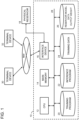
- FIG. 1 is a schematic diagram of an information processing system for realizing a reservoir computing model according to the present embodiment.
- An information processing device 10 is a computer such as a PC or an HPC, for example.
- the information processing device 10 includes a processor 12, a main memory 14 that is accessed by the processor, and an interface device 16 that communicates with the outside.
- a training program 20 for a reservoir model, an inference program 22, training data 24 used in the training, and reservoir model data 26 including configuration data of the reservoir model and parameters such as output weights are stored in large-capacity auxiliary storage devices 20 to 26 of the information processing device 10.
- the processor 12 executes calculations of a training process and calculations of an inference process by executing the training program 20 and the inference program 22, which are read from the auxiliary storage devices and expanded in the main memory 14. Further, the processor 12 calculates transitions in the state of the reservoir in response to time series input by executing a calculation program included in the reservoir model data 26.
- the information processing system of FIG. 1 may be provided with a physical reservoir 18.
- the processor 12 refers to physical changes in the physical reservoir 18 via the interface 16 instead of calculating the state transitions of the reservoir by referring to the reservoir model data 26.
- the processor 12 instead acquires the output of the physical reservoir 18 and updates the output weights by calculation so as to reduce an error between teaching data and the output.
- the information processing device 10 is accessed from a plurality of terminal devices 30, 32 via a network NW.
- the processor 12 executes calculations of a training model or an inference model and thereby executes calculations of the requested training processing or inference processing.
- FIG. 2 is a view depicting an example of a network of a reservoir computing model. Neurons of the reservoir will be referred to hereinafter as nodes.
- a reservoir RSV includes nodes N1 to N5 and inter-node connections and node self-connections. The connections are known as edges. Further, the connections each have a direction indicated by an arrow and a weight corresponding to the direction. In the figure, the arrows inside the reservoir RSV denote inter-node connections or node self-connections. For example, the nodes N1 and N3 are self-connected. A bidirectional connection exists between the node N1 and the node N2. A single-direction connection from the node N2 to the node N3 exists between the nodes N2 and N3.
- the inter-node connections or self-connections and the weights of the respective connections in the reservoir RSV are determined prior to training either at random or in accordance with a predetermined rule.
- the predetermined rule means connection probabilities between the nodes and the weight distribution of the connections as parameters.
- the states of the nodes N1 to N5 transition based on the input and the states of the nodes at a time prior to the time t.
- the states of the nodes N4 and N5 are output, whereupon an activation calculated based on the outputs (the readouts) of the nodes N4 and N5 and output weights w4, w5 is input into an output terminal OUT.
- the nodes N4 and N5, the connections of the output weights w4, w5, and the output terminal OUT constitute a fully connected layer FCL.
- the reservoir computing model includes the reservoir RSV and a readout portion forming the fully connected layer FCL for the output of the reservoir.
- the node N1 corresponds to an input layer to which the input is applied, and the nodes N4 and N5 correspond to an output layer from which the states thereof are read as output.
- the nodes N2 and N3 between the node N1 of the input layer and the nodes N4, N5 of the output layer correspond to an middle layer.
- the output weight of the fully connected layer FCL serving as the readout portion is updated in accordance with the gradient method while keeping the inter-node connections and node self-connections in the reservoir fixed.
- the output weights w4, w5 are updated by the gradient method so as to minimize the error between the teaching data and the output of the output node OUT.
- the weights of the connections in the reservoir are not updated by the gradient method during the training process.
- the number of output weights that are adjusted by being updated in the gradient method is small, and therefore the training processing is simplified. As a result, the training process is completed with a smaller amount of training data.
- the reservoir computing model either the reservoir RSV is realized by a physically configured physical reservoir, or the state transitions of the reservoir is calculated by calculations performed by a computer program.
- An example of a crossbar reservoir that uses nonlinear elements will be described below as an example of a physical reservoir.
- FIG. 3 is a view depicting an information processing system using a crossbar reservoir, which is a type of physical reservoir, as a reservoir computing model.
- the information processing system of the reservoir computing model depicted in FIG. 3 includes an information processing device 10 having a processor, and a crossbar reservoir C_RSV serving as a physical reservoir.
- the crossbar reservoir C_RSV includes column lines corresponding to node inputs, and row lines corresponding to node outputs, and although not illustrated in the figure, physical circuits such as memristors, CR circuits, or other analog circuits having nonlinearity are provided between the column lines and row lines.
- the input IN1 is supplied to the input of the node N1 of the input layer in the crossbar reservoir C_RSV from the processor, and the outputs (the readout values) of the nodes N4, N5 of the output layer are output to the processor.
- the processor executes the calculations of the training process and the inference process on the fully connected layer serving as the readout portion by executing a computer program.
- the processor that executes the training program supplies the input IN1, which is constituted by training data, to the node N1 serving as the input layer of the crossbar reservoir C_RSV, and in response thereto, the state of the crossbar reservoir C_RSV transitions from a past state to the current state.
- the processor receives input of output indicating the states of the nodes N4, N5 serving as the output layer of the crossbar reservoir C_RSV, and by executing the training program updates the output weights W4, W5 of the fully connected layer FCL serving as the readout portion by means of the gradient method.
- the output weights are optimized, whereby a reservoir computing model that generates output that is identical or close to the teaching of the training data is generated.
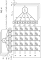
- FIG. 4 is a view depicting an example of a crossbar reservoir and an example of a fully connected layer serving as the readout portion.
- the crossbar reservoir C_RSV includes, in relation to the five nodes N1 to N5 illustrated in FIG. 2 , five column lines (vertical lines) N1 to N5 corresponding to the inputs of the nodes, five row lines (horizontal lines) N1 to N5 corresponding to the outputs of the nodes, and 25 connection circuits f11 to f55 arranged at the intersections between the column lines and the row lines.
- the connection circuits f11 to f55 are memristors, for example.
- connection circuits f11 to f55 are provided between all the five column lines and five row lines, but the connection circuits may be provided only between certain column lines and row lines.
- inter-node connections and node self-connections are provided between and in only some of the nodes respectively.
- a connection circuit between the column line and the row line of the same node corresponds to a node self-connection.
- a connection circuit between the column line and the row line of different nodes corresponds to a single direction inter-node connection from the node of the column line in the direction of the node of the row line.
- the connection circuits correspond to the weights of the connections in the reservoir of FIG. 2 .
- analog signals X1 to X5 acquired by converting digital signals supplied from the input terminal IN1 of an input portion IN_1 using a DAC are input into the five column lines corresponding to the inputs of the nodes. This occurs similarly in input portions IN_2, IN_3. Note that when inputs are applied to some of the nodes in the reservoir, the analog signals acquired by converting the digital signals of the input terminal IN1 using a DAC are applied to the inputs of some of the nodes.
- analog signals y1 to y5 of the five row lines corresponding to the outputs of the nodes are converted using an ADC (analog-digital converter) and output to a fully connected layer FCL_1, whereupon a digital signal of a product sum value generated by the fully connected layer FCL_1 is output to an output node OUT1 as an activation.
- f11, f12, f21, f24, f32, f33, f35, f45, f51, and f54 have finite values, while the remainder are infinite, or in other words unconnected.
- this type of crossbar reservoir C_RSV when the input x1, among time series inputs, is applied to the node N1 of the input layer at a time t1, the states of all the nodes N1 to N5 transition to the outputs y1 to y5 as illustrated in the following formula.
- f11(x) to f55(x) are functions for determining the values to be output to the outputs y of the nodes in relation to the inputs x of the nodes.
- a time t0 is a time one interval before the time t1 that is the input time
- y1_t1 is the state at the time t1
- y1_t0 is the state at the time t0.
- ⁇ corresponds to the decay rate of the state of a node.
- each node successively transitions to a new state in response to time series input while maintaining a state based on past input.
- the input is non-linearly transformed by the crossbar reservoir C_RSV, and the state following transformation is mapped to a high-dimensional feature space.
- the states of the nodes on the output layer of the crossbar reservoir C_RSV are linearly connected in the fully connected layer FCL, whereupon the output OUT is output.
- an adjacency matrix illustrating the weights of the inter-node connections and node self-connections of the crossbar reservoir C_RSV on a matrix.
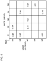
- FIG. 5 is a view depicting an example of an adjacency matrix of a crossbar reservoir corresponding to the example of FIG. 2 .
- the weights of the inter-node connections and the weights of the node self-connections are indicated in intersection positions between columns corresponding to the inputs of the nodes N1 to N5 and rows corresponding to the outputs of the nodes N1 to N5.
- the weight of the self-connection of the node N1 is indicated in the intersection position between the column of the node N1 and the row of the node N1.
- weight of the inter-node connection from the node N1 to the node N2 is indicated in the intersection position between the column of the node N1 and the row of the node N2.
- weight of the inter-node connection from the node N2 to the node N1 is indicated in the intersection position between the column of the node N2 and the row of the node N1.
- weights are indicated respectively in the positions of the functions f11, f12, f21, f24, f32, f33, f35, f45, f51, and f54 depicted in the above formula.
- FIG. 6 is a view illustrating connections on the intersections of an adjacency matrix of a crossbar reservoir are classified into types.
- the node N1 is an input layer INL
- the nodes N4, N5 are an output layer OUTL
- the nodes N2, N3 between the input layer and the output layer are a middle layer MIDL.
- the intersection position between the column and the row of the node N1 indicates the input layer INL
- the intersection positions between the column and the row of the nodes N4, N5 indicate the output layer OUTL
- the intersection positions between the column and the row of the nodes N2, N3 indicate the middle layer MIDL.
- the input layer INL, the middle layer MIDL, and the output layer OUTL form a square matrix having the number of nodes constituting the respective layers, and correspond to node self-connection areas.
- intersection positions between the column of the node N1 and the row of N2, N3 indicate an inter-node connection area I_M from the input layer to the middle layer
- intersection positions between the column of the nodes N2, N3 and the row of the nodes N4, N5 indicate an inter-node connection area M_O from the middle layer to the output layer
- intersection positions between the column of the nodes N2, N3 and the row of the node N1 indicate an inter-node connection area M_I from the middle layer to the input layer
- intersection positions between the column of the nodes N4, N5 and the row of the nodes N2, N3 indicates an inter-node connection area O_M from the output layer to the middle layer
- intersection positions between the column of the node N1 and the row of the nodes N4, N5 indicate an inter-node connection area I_O from the input layer to the output layer
- intersection positions between the column of the nodes N4, N5 and the row of the node N1 indicate an inter-node connection area I_
- FIG. 7 is a view depicting relationships between the nine areas illustrated on the adjacency matrix of FIG. 6 .
- FIG. 7 illustrates relationships between the input layer INL, middle layer MIDL, and output layer OUTL and the inter-node connection areas I_M, M_O, I_O, O_M, M_I, and I_O therebetween.
- the node N1 of the input layer INL transitions to the sum of change in N1 caused by the input x1 at the time t1, change in N1 based on the node state x1 of the input layer INL at the time t0 and the self-connection thereof, and change in N1 based on the node states x2, x3 of the middle layer MIDL at the time t0 and the inter-node connection M_I (N2, N3 to N1) of the area M_I of N1.
- the nodes N2, N3 of the middle layer MIDL transition to the sum of change in N2, N3 based on the input x1 to N1 at the time t1 and the inter-node connection (N1 to N2, N3) of the area I_M, change in N2, N3 based on the node states x2, x3 of the middle layer MIDL at the time t0 and the self-connection of the middle layer, and change in N2, N3 based on the node states x4, x5 of the output layer OUTL at the time t0 and the inter-node connection (N4, N5 to N2, N3) of the area O_M.
- the input layer INL, the middle layer MIDL, and the output layer OUTL of the crossbar reservoir form square-shaped areas within an adjacency matrix and each have a self-connection. Further, the inter-node connections between the layers are positioned in the areas I_M, M_O, O_M, M_I, I_O, and O_I of the adjacency matrix.
- the reservoir takes on the characteristics of a higher-dimensional function.
- overtraining occurs, and as a result, the model enters an overfitted state.
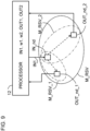
- FIG. 8 is a view depicting a reservoir computing model according to a first embodiment.
- the model of FIG. 8 is an information processing system including the crossbar reservoir C_RSV, which serves as an example of a physical reservoir, and the information processing device 10.
- the crossbar reservoir C_RSV includes a first partial reservoir C_RSV_1, and a second partial reservoir C_RSV_2 in which the size between the input layer and the output layer is larger than in the first partial reservoir, whereby the second partial reservoir C_RSV_2 has a function characteristic of a higher dimension than the first partial reservoir C_RSV_1.
- the first partial reservoir C_RSV_1 and the second partial reservoir C_RSV_2 share a common input node IN_nd, have respective output nodes OUT_nd_1, OUT_nd_2, and have respective middle layer nodes between the common input node and the respective output nodes.
- the common input node IN_nd constitutes a common input layer
- the output nodes OUT_nd_1, OUT_nd_2 constitute respective output layers.
- the configuration of the crossbar reservoir C_RSV will be described below using an adjacency matrix.
- the size of the reservoir corresponds to the number of nodes on the middle layer, for example.
- Readout values from the output nodes OUT_nd_1, OUT_nd_2 of the respective output layers are output to the information processing device 10 illustrated in FIG. 1 , whereupon the processor 12 calculates a product sum value of the linear connection of the readout values and the output weights so as to generate two outputs OUT1, OUT2, and calculates the sum of the two outputs as the output of the crossbar reservoir C_RSV. Further, the processor 12 optimizes the output weights using training data in a training process, the procedures of which will be described below.
- FIG. 9 is a view depicting a reservoir computing model according to a second embodiment.
- the model of FIG. 9 is an information processing system including a material reservoir M_RSV that uses the nonlinearity of a material and is an example of a physical reservoir, and the information processing device 10.
- material reservoirs include, for example, a mass of material having electrical non-linearity, a mass of material having optical non-linearity, and so on.
- the material reservoir M_RSV is a mass of material.
- the material between the nodes of the input layer and the output layer constitute virtual nodes of a middle layer.
- the material reservoir M_RSV includes a first partial reservoir M_RSV_1 and a second partial reservoir M_RSV_2 in which the size between the input layer and the output layer is larger than in the first partial reservoir M_RSV_1, whereby the second partial reservoir M_RSV_2 has a function characteristic of a higher dimension than the first partial reservoir M_RSV_1.
- the first partial reservoir M_RSV_1 and the second partial reservoir M_RSV_2 include a partially overlapping area, and the input node IN_nd of the common input layer is provided therein. Further, the nodes OUT_nd_1, OUT_nd_2 of the output layers are provided respectively in the first partial reservoir M_RSV_1 and the second partial reservoir M_RSV_2.
- the size of the material reservoir M_RSV corresponds to the distance between the input node IN_nd and the output node OUT_nd, for example.
- readout values from the output nodes OUT_nd_1, OUT_nd_2 of the respective output layers are output to the information processing device 10, whereupon the processor calculates a product sum value of the linear connections of the readout values and the output weights so as to generate the two outputs OUT1, OUT2, and calculates the sum of the two outputs as the output of the material reservoir M_RSV.
- the processor also optimizes the output weights using training data in a training process, the procedures of which will be described below.
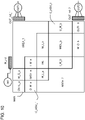
- FIG. 10 is a view depicting areas of an adjacency matrix of the reservoir computing model according to the first embodiment.
- the crossbar reservoir C_RSV that is an example of a physical reservoir includes the first partial reservoir C_RSV_1 and the larger second partial reservoir C_RSV_2.
- FIG. 11 is a view depicting relationships between the nine areas illustrated on the adjacency matrix of FIG. 10 .
- the first partial reservoir C_RSV_1 includes the input layer INL having the input node IN_nd, a first output layer OUTL_a having the first output node OUT nd_1, and a first middle layer MIDL_a having a first group of intermediate nodes therebetween.
- the first partial reservoir C_RSV_1 includes an area I_M_a that includes an inter-node connection from the node of the input layer INL to the nodes of the first middle layer MIDL_a, and an area M_O_a that includes an inter-node connection from the nodes of the first middle layer MIDL_a to the node of the first output layer OUTL_a.
- the first partial reservoir C_RSV_1 includes an area O_M_a that includes an inter-node connection from the node of the output layer OUTL to the nodes of the first middle layer MIDL_a, and an area M_I_a that includes an inter-node connection from the nodes of the first middle layer MIDL_a to the node of the input layer INL.
- areas I_O_a and O_I_a within areas AREA_1 and AREA_2 of FIG. 10 the inter-node connections are unconnected. The reason for this is that in the case of a physical reservoir, the distance between the input node group and the output node group is typically long, and therefore these inter-node connections are unconnected.
- the product sum value of the readout value of the first output node OUT_nd_1 of the first output layer and the output weight forms the first output OUT1.
- the output weight of this fully connected layer is updated to an optimum value in the training process.
- the second partial reservoir C_RSV_2 includes the input layer INL having the input node IN_nd, a second output layer OUTL_b having the second output node OUT_nd_2, and a second middle layer MIDL_b having a second group of intermediate nodes therebetween.
- the second partial reservoir C_RSV_2 includes an area I_M_b that includes an inter-node connection from the node of the input layer INL to the nodes of the second middle layer MIDL_b, and an area M_O_b that includes an inter-node connection from the nodes of the second middle layer MIDL_b to the node of the second output layer OUTL_b.
- the second partial reservoir C_RSV_2 includes an area O_M_b that includes an inter-node connection from the node of the output layer OUTL to the nodes of the second middle layer MIDL_b, and an area M_I_b that includes an inter-node connection from the nodes of the second middle layer MIDL_b to the node of the input layer INL. Note that in areas I_O_b and O_I_b within the areas AREA_1 and AREA_2 of FIG. 10 , the inter-node connections are unconnected. The reason for this is as described above.
- the product sum value of the readout value of the second output node OUT_nd_2 of the second output layer and the output weight forms the second output OUT2.
- the output weight of this fully connected layer is updated to an optimum value in the training process.
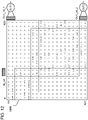
- FIG. 12 is a view depicting a specific example of an adjacency matrix.
- This adjacency matrix NMX is a 20 ⁇ 20 matrix and therefore an adjacency matrix corresponding to a crossbar reservoir with 20 nodes.
- the crossbar reservoir having 20 nodes is divided into an input node group of nodes N7, N8, a first output node group N1, N2, a second output node group N19, N20, a first intermediate node group N3 to N6, and a second intermediate node group N9 to N18.
- a first partial reservoir includes the input node group N7, N8 (IN_nd), the first output node group N1, N2, and the first intermediate node group N3 to N6.
- the product sum value of the readout values of the first output node group N1, N2 (OUT _nd_1) and the output weights is the first output OUT1.
- a second partial reservoir includes the input node group N7, N8 (IN_nd), the second output node group N19, N20 (OUT_nd_2), and the second intermediate node group N9 to N18.
- the product sum value of the readout values of the second output node group N19, N21 and the output weights is the second output OUT2.
- the initial weights set in the intersection positions of the crossbar reservoir are designed as appropriate in accordance with the object to be realized by the reservoir computing model.
- the adjacency matrices of FIGS. 10 , 11 , and 12 can also be applied to a material reservoir.
- a material reservoir generates a nonlinear readout value in the output node in response to input applied to the input node, and therefore, by setting the weights so as to correspond to this nonlinearity, it is possible to design an adjacency matrix of a reservoir having a target nonlinearity.
- FIG. 13 is a flowchart illustrating a training process executed on the reservoir computing models of the first and second embodiments.
- the processor executes the following processing by executing the training program.
- the processor initializes the output weight of the reservoir (S1).
- the processor inputs an input value of the training data into the input node of the reservoir (S2).
- the first partial reservoir which has a smaller number of nodes or a smaller size, generates states of the respective nodes based on the input value, past node states, and the inter-node connections and node self-connections (S3).
- the second partial reservoir in which the number of nodes between the input layer and the output layer is larger than in the first partial reservoir or the size between the input layer and the output layer is larger than in the first partial reservoir, generates states of the respective nodes based on the input value, past node states, and the inter-node connections and node self-connections (S4).
- the respective states of the first partial reservoir and the second partial reservoir transition, whereby the states of the first output node of the first partial reservoir and the second output node of the second partial reservoir transition.
- the aforesaid state transitions of the first partial reservoir and second partial reservoir may also be achieved by having the processor calculate the states of the first output node of the first partial reservoir and the second output node of the second partial reservoir by calculating the state transitions of the first and second partial reservoirs.
- the processor executes first parameter adjustment for adjusting the output weight of the first partial reservoir to an optimum value (S5).
- the processor updates the first output weight so as to reduce the difference between the first output and the teaching data.
- the output weight can be updated using the gradient method or learn the output weight using a simple algorithm such as linear regression.
- the processor sets the first output weight of the first partial reservoir at the updated value, calculates the first output relative to the input value of step S2, and calculates the difference between the first output and the teaching data as differential teaching data (S6).
- the processor executes second parameter adjustment for adjusting the output weight of the second partial reservoir to an optimum value (S7).
- the processor updates the second output weight so as to reduce the difference between the second output and the differential teaching data. Updating of this output weight of the second partial reservoir is identical to that of the first partial reservoir except that the differential teaching data is used in the second partial reservoir, not the teaching data.
- the processor executes the processing from step S2, in which the input value of the training data is input, to step S7, i.e., the second parameter adjustment, repeatedly on all the training data (S8).
- the processing is executed repeatedly on a plurality of training data until the output accuracy of the model reaches a target accuracy.
- the output accuracy of the model is determined by dividing the difference between the sum of the first output of the readout portion of the first partial reservoir and the second output of the readout portion of the second partial reservoir and the teaching data by this sum, or the like.
- the first partial reservoir and the corresponding readout portion having been optimized by the training, generate a first output of a low-frequency component. Since the function is low-dimensional, overtraining can be avoided in the training process.
- the second partial reservoir has a larger size and a larger number of nodes than the first partial reservoir, and therefore the second partial reservoir generates a function model of a higher dimension than the first partial reservoir.
- the second partial reservoir and the corresponding readout portion having been optimized by the training, generate a second output of a high-frequency component.
- the sum of the first output and the second output is the output of the reservoir computing model.
- the reservoir computing model is capable of generating an output in which the second output of the high-frequency component is added to the first output of the low-frequency component.
- FIG. 14 is a flowchart illustrating the processing of an inference process performed by the reservoir computing models according to the first and second embodiments.
- the processor inputs an input value into the reservoir (S10).
- the respective states of the first partial reservoir which has a small number of nodes and a small size
- the second partial reservoir which has a large number of nodes and a large size, transition based on the input value, the states of the respective reservoirs corresponding to the past input history, and the inter-node connections and node self-connections (S11, S12).
- the processor calculates the first output of the readout portion based on the value of the output node and the output weight of the first partial reservoir (S13), and calculates the second output of the readout portion based on the value of the output node and the output weight of the second partial reservoir (S14).
- the output weights at this time are the optimal output weights adjusted in the training process.
- the processor then calculates an inference value by calculating the sum of the first output and the second output (S15).
- the processor repeats the inference process S10 to S15 described above until inference is complete (S16).
- the processor similarly to the training process, the processor generates a low-frequency component of the inference output using the first partial reservoir and the readout portion thereof, and generates a high-frequency component of the inference output using the second partial reservoir and the readout portion thereof.
- the training process does not produce an overtrained state, and therefore a highly generalized reservoir computing model can be generated.
- FIG. 15 is a flowchart of FORCE learning for updating the output weights of the training process.
- FORCE learning First Order Reduced and Controlled Error Learning
- the processor inputs a reservoir output vector (a vector of the readout value output by the output node) r(t) and teaching data f(t) (S20).
- the reservoir output vector r(t) is a matrix of 1 row and n columns at a time t, and the readout values of the n output nodes form n elements on the matrix.
- the processor initializes a matrix P(t) and an output weight w(t) (S22, S23).
- the matrix P is a matrix for calculating an output weight vector w(t) and is initialized by means of a unit matrix I.
- a difference e is then updated (S26).
- the processor inputs the reservoir output vector r(t) and the teaching data f(t) (S20), and since this is not the first time (NO in S21), the processor updates the matrix P and the output weight w(t) (S24, S25). Calculation formulae for the respective updates are illustrated in FIG. 15 .
- the processor calculates the matrix P(t) of the current time t from a matrix P(t- ⁇ t) of an immediately preceding time t- ⁇ t using the calculation formula indicated in S24 (S24).
- the processor calculates the output weight w(t) of the current time t from an output weight w(t- ⁇ t) of the immediately preceding time t- ⁇ t using the calculation formula indicated in S25 (S25).
- the processor then updates the difference e (S26).
- the processor performs a multiply-accumulate operation by multiplying the reservoir output vector r(t) of the current time t by a transposed matrix of the output weight w updated at the current time t, and then outputs the difference between the multiply-accumulate operation value and the teaching data f(t) as the difference e(t) at the current time t.
- the processor repeats the processing for updating the output weight w(t) by executing steps S24 to S26 each time new training data and a new reservoir output vector are input.
- the processing for updating the output weight described above, is performed in the processing S5 for updating the output weight of the readout portion of the first partial reservoir and the processing S7 for updating the output weight of the readout portion of the second partial reservoir, illustrated in FIG. 13 .
- differential teaching data are used as the training data.
- FIG. 16 is a view depicting a reservoir computing model according to a third embodiment.
- the model of FIG. 16 similarly to FIG. 9 , is an information processing system including the material reservoir M_RSV and the information processing device 10.
- the material reservoir M_RSV includes the first partial reservoir M_RSV_1, the second partial reservoir M_RSV_2 that has a larger size and a function characteristic of a higher dimension than the first partial reservoir M_RSV_1, and a third partial reservoir M_RSV_3 that has a larger size and a function characteristic of a higher dimension than the second partial reservoir M_RSV_2.
- the first partial reservoir M_RSV_1, second partial reservoir M_RSV_2, and third partial reservoir M_RSV_3 have a partially overlapping area, and the input node IN_nd of the common input layer is provided therein. Further, the nodes OUT_nd_1, OUT_nd_2, OUT_nd_3 of the output layers are provided respectively in the first, second, and third partial reservoirs M_RSV_1, M_RSV_2, and M_RSV_3.
- the readout values from the output nodes OUT_nd_1, OUT_nd_2, OUT_nd_3 of the respective output layers are input into the information processing device 10, whereupon the processor 12 calculates product sum values constituted by linear combinations of the readout values and the output weights, thereby generating three outputs OUT1, OUT2, and OUT3, and calculates the sum thereof as the output of the crossbar reservoir.
- the processor optimizes the output weights by using the training data in the training process.
- the input value of the training data is input into the input node IN_nd, whereupon the states of the three partial reservoirs are caused to transition and the weights of the respective readout portions of the three partial reservoirs are updated in increasing order of size from the partial reservoir having the smallest size.
- the difference between the first output, which is calculated based on the updated output weight of the readout portion of the first partial reservoir, and the teaching data is set as differential teaching data.
- the difference between a sum of the first output, which is calculated based on the updated output weight of the readout portion of the first partial reservoir, and the second output of the second partial reservoir, which is similar to the first output, and the teaching data is set as differential teaching data.
- the processor outputs the sum of the first, second, and third outputs corresponding respectively to the three partial reservoirs as the output of the material reservoir.
- the crossbar reservoir of FIG. 8 was realized by having a processor execute a state transition calculation program for a crossbar reservoir.
- An example of the weights of the inter-node connections and self-connections and the input node and two output nodes of the crossbar reservoir is similar to FIG. 12 , for example. Note, however, that contrast to the 20 nodes of FIG. 12 , in this example, the number of nodes was set at 100, i.e., five times more than FIG. 12 .
- the processor was configured to execute a state transition calculation program for a case in which circuit elements such as nonlinear memristors were provided on the intersections of the crossbar structure.
- 10 input nodes, 10 first output nodes, and 10 second output nodes were provided, while the number of nodes on the first middle layer of the first partial reservoir was set at 20 and the number of nodes on the second middle layer of the second partial reservoir was set at 50.
- the inter-node connections and self-connections of the crossbar reservoir were chosen at random, and connections between distant nodes, such as the input node and the output node, were left unconnected.
- a reservoir not divided into a plurality of partial reservoirs was used, and a reservoir model in which the total number of nodes was set at 100, with 10 input nodes, 10 output nodes, and 80 nodes on the middle layer, was employed.
- NARMA10 is generally known as a method for evaluating an RNN.
- the nonlinear function of NARMA10 outputs time-series numerical value data in response to the input of time-series input data of a certain length.
- the input and the output time-series numerical value data serve as the input data of the training data and the teaching data.
- the input data of the training data described above were input in time series into the reservoir computing model of the example, and using corresponding teaching data, training for optimizing the output weight of the model was executed repeatedly. Then, the normalized root-mean-square deviation (NRMSE) of an error between the output data generated by the model when the input data of NARMA10 were applied to the trained model and correct answer data output by the function of NARMA10 was calculated. Further, the reservoir model of the comparative example was trained in a similar manner, whereupon the error after the training was calculated. As a result, the error in the reservoir model of the comparative model was 0.2033, whereas the error in the reservoir model according to this embodiment was 0.1718, i.e., smaller than that of the comparative example.
- a common input is input into a plurality of partial models having successively larger reservoir sizes, whereupon training is performed to update the output weights of the readout portions of the respective partial reservoirs in ascending order of size so as to reduce the difference between the output and the teaching data.
- the respective output weights are updated so that in the first partial reservoir having the smallest size and the readout portion thereof, the difference between the first output of the readout portion and the teaching data is reduced, in the second partial reservoir having the next smallest size and the readout portion thereof, the difference between the second output of the readout portion and differential training data (a value acquired by subtracting the first output calculated based on the updated output weight from the teaching data) is reduced, and in a Kth partial reservoir and the readout portion thereof, the difference between the Kth output of the readout portion and differential training data (a value acquired by subtracting the sum of first to K-1th outputs calculated based on the updated output weights from the teaching data) is reduced.
- the reservoir computing model is configured such that the partial reservoir having the smallest size and the readout portion thereof generate the lowest-wavelength component of the output, while the higher-wavelength components of the output are generated in increasing order of size.
Landscapes
- Engineering & Computer Science (AREA)
- Physics & Mathematics (AREA)
- Theoretical Computer Science (AREA)
- General Physics & Mathematics (AREA)
- Health & Medical Sciences (AREA)
- Life Sciences & Earth Sciences (AREA)
- Biomedical Technology (AREA)
- Biophysics (AREA)
- General Engineering & Computer Science (AREA)
- Computing Systems (AREA)
- Molecular Biology (AREA)
- Software Systems (AREA)
- Evolutionary Computation (AREA)
- Data Mining & Analysis (AREA)
- Computational Linguistics (AREA)
- Artificial Intelligence (AREA)
- Mathematical Physics (AREA)
- General Health & Medical Sciences (AREA)
- Neurology (AREA)
- Computational Mathematics (AREA)
- Mathematical Analysis (AREA)
- Pure & Applied Mathematics (AREA)
- Mathematical Optimization (AREA)
- Complex Calculations (AREA)
- Multi Processors (AREA)
Applications Claiming Priority (1)
| Application Number | Priority Date | Filing Date | Title |
|---|---|---|---|
| PCT/JP2020/015877 WO2021205581A1 (ja) | 2020-04-08 | 2020-04-08 | 情報処理システム、情報処理装置、情報処理方法及び情報処理プログラム |
Publications (2)
| Publication Number | Publication Date |
|---|---|
| EP4134882A1 true EP4134882A1 (de) | 2023-02-15 |
| EP4134882A4 EP4134882A4 (de) | 2023-05-10 |
Family
ID=78023581
Family Applications (1)
| Application Number | Title | Priority Date | Filing Date |
|---|---|---|---|
| EP20930582.0A Pending EP4134882A4 (de) | 2020-04-08 | 2020-04-08 | Informationsverarbeitungssystem, informationsverarbeitungsvorrichtung, informationsverarbeitungsverfahren und informationsverarbeitungsprogramm |
Country Status (5)
| Country | Link |
|---|---|
| US (1) | US12596927B2 (de) |
| EP (1) | EP4134882A4 (de) |
| JP (1) | JP7376832B2 (de) |
| CN (1) | CN115443473A (de) |
| WO (1) | WO2021205581A1 (de) |
Cited By (1)
| Publication number | Priority date | Publication date | Assignee | Title |
|---|---|---|---|---|
| US12620996B2 (en) | 2022-11-28 | 2026-05-05 | Tdk Corporation | Signal processor with A-D converter and reservoir unit |
Families Citing this family (2)
| Publication number | Priority date | Publication date | Assignee | Title |
|---|---|---|---|---|
| CN115378814B (zh) * | 2022-08-22 | 2024-12-31 | 中国科学院微电子研究所 | 一种储备池计算网络优化方法及相关装置 |
| CN117744644B (zh) * | 2023-12-20 | 2025-01-07 | 北京百度网讯科技有限公司 | 数据处理方法、数据处理模型及其训练方法 |
Family Cites Families (9)
| Publication number | Priority date | Publication date | Assignee | Title |
|---|---|---|---|---|
| JP4093858B2 (ja) | 2000-10-13 | 2008-06-04 | フラウンホーファー−ゲゼルシャフト・ツア・フォルデルング・デア・アンゲヴァンテン・フォルシュング・エー・ファウ | リカレントニューラルネットワーク |
| JP5157359B2 (ja) * | 2006-10-10 | 2013-03-06 | オムロン株式会社 | 時系列データ解析装置、時系列データ解析システム、時系列データ解析装置の制御方法、プログラム、および記録媒体 |
| US9165246B2 (en) * | 2013-01-29 | 2015-10-20 | Hewlett-Packard Development Company, L.P. | Neuristor-based reservoir computing devices |
| US10395168B2 (en) * | 2015-10-26 | 2019-08-27 | International Business Machines Corporation | Tunable optical neuromorphic network |
| US11188818B2 (en) * | 2017-04-03 | 2021-11-30 | International Business Machines Corporation | Reservoir computing system |
| JP6791800B2 (ja) | 2017-04-05 | 2020-11-25 | 株式会社日立製作所 | 計算機システム及び再帰型ニューラルネットワークを用いた演算方法 |
| WO2018212201A1 (ja) | 2017-05-15 | 2018-11-22 | 国立大学法人大阪大学 | 情報処理装置及び情報処理方法 |
| CN109009033A (zh) * | 2018-07-10 | 2018-12-18 | 华南理工大学 | 一种基于小波分析和回声状态网络的血压预测方法 |
| CN109640351A (zh) * | 2019-01-25 | 2019-04-16 | 南京邮电大学 | 一种基站流量的联合预测方法 |
-
2020
- 2020-04-08 EP EP20930582.0A patent/EP4134882A4/de active Pending
- 2020-04-08 JP JP2022513781A patent/JP7376832B2/ja active Active
- 2020-04-08 WO PCT/JP2020/015877 patent/WO2021205581A1/ja not_active Ceased
- 2020-04-08 CN CN202080099442.XA patent/CN115443473A/zh active Pending
-
2022
- 2022-10-03 US US17/958,476 patent/US12596927B2/en active Active
Cited By (1)
| Publication number | Priority date | Publication date | Assignee | Title |
|---|---|---|---|---|
| US12620996B2 (en) | 2022-11-28 | 2026-05-05 | Tdk Corporation | Signal processor with A-D converter and reservoir unit |
Also Published As
| Publication number | Publication date |
|---|---|
| EP4134882A4 (de) | 2023-05-10 |
| WO2021205581A1 (ja) | 2021-10-14 |
| JPWO2021205581A1 (de) | 2021-10-14 |
| JP7376832B2 (ja) | 2023-11-09 |
| US20230023123A1 (en) | 2023-01-26 |
| CN115443473A (zh) | 2022-12-06 |
| US12596927B2 (en) | 2026-04-07 |
Similar Documents
| Publication | Publication Date | Title |
|---|---|---|
| US12596927B2 (en) | Information processing system having an information processing device and multiple partial reservoirs that are trained, information processing device that trains multiple partial reservoirs, and non-transitory computer readable memory medium that stores information processing program for training multiple partial reservoirs | |
| CN107924227B (zh) | 电阻处理单元 | |
| Tsai et al. | Tuning the structure and parameters of a neural network by using hybrid Taguchi-genetic algorithm | |
| US5165009A (en) | Neural network processing system using semiconductor memories | |
| KR20040099092A (ko) | 계기 노이즈 및 측정 오차의 존재 하의 인공 신경망모델의 향상된 성능 | |
| Suykens et al. | NL/sub q/theory: checking and imposing stability of recurrent neural networks for nonlinear modeling | |
| Stoop et al. | Beyond scale-free small-world networks: cortical columns for quick brains | |
| CN111077768A (zh) | 优化装置及优化装置的控制方法 | |
| Takatani et al. | Neural network-based construction of inverse kinematics model for serial redundant manipulators | |
| JP2021119425A (ja) | モデル生成装置、モデル生成方法及びプログラム | |
| CN109670582B (zh) | 一种全定点化神经网络的设计方法 | |
| Yang et al. | A neural network learning algorithm of chemical process modeling based on the extended Kalman filter | |
| KR102607864B1 (ko) | 뉴로모픽 시스템 및 그것의 동작 방법 | |
| Salvi et al. | Long short-term model for Brent oil price forecasting | |
| JP2001117900A (ja) | ニューラルネットワーク演算装置 | |
| US20210173978A1 (en) | Optimization device, optimization device control method, and computer-readable recording medium recording optimization device control program | |
| JP2021189532A (ja) | パターン認識装置、学習方法及び学習プログラム | |
| Starzyk et al. | Artificial neural network for testing analog circuits | |
| CN117610636A (zh) | 一种存内计算存储器人工神经网络的片上训练方法 | |
| KR20210113722A (ko) | 트랜스포즈 매트릭스 곱셈이 가능한 매트릭스 곱셈기 구조 및 곱셈방법 | |
| US12353983B2 (en) | Inference device and method for reducing the memory usage in a weight matrix | |
| JPH05197705A (ja) | ニューラルネットワークの学習システム | |
| JP2023027851A (ja) | 訓練装置、プラント、モデルを生成する方法、推論装置、推論方法及びプラントの制御方法 | |
| WO2024116229A1 (ja) | 信号処理装置 | |
| Merolla et al. | The thermodynamic temperature of a rhythmic spiking network |
Legal Events
| Date | Code | Title | Description |
|---|---|---|---|
| STAA | Information on the status of an ep patent application or granted ep patent |
Free format text: STATUS: THE INTERNATIONAL PUBLICATION HAS BEEN MADE |
|
| PUAI | Public reference made under article 153(3) epc to a published international application that has entered the european phase |
Free format text: ORIGINAL CODE: 0009012 |
|
| STAA | Information on the status of an ep patent application or granted ep patent |
Free format text: STATUS: REQUEST FOR EXAMINATION WAS MADE |
|
| 17P | Request for examination filed |
Effective date: 20221005 |
|
| AK | Designated contracting states |
Kind code of ref document: A1 Designated state(s): AL AT BE BG CH CY CZ DE DK EE ES FI FR GB GR HR HU IE IS IT LI LT LU LV MC MK MT NL NO PL PT RO RS SE SI SK SM TR |
|
| REG | Reference to a national code |
Ref country code: DE Ref legal event code: R079 Free format text: PREVIOUS MAIN CLASS: G06N0020000000 Ipc: G06N0003044000 |
|
| A4 | Supplementary search report drawn up and despatched |
Effective date: 20230412 |
|
| RIC1 | Information provided on ipc code assigned before grant |
Ipc: G06N 3/09 20230101ALI20230404BHEP Ipc: G06N 3/045 20230101ALI20230404BHEP Ipc: G06N 3/065 20230101ALI20230404BHEP Ipc: G06N 3/044 20230101AFI20230404BHEP |
|
| DAV | Request for validation of the european patent (deleted) | ||
| DAX | Request for extension of the european patent (deleted) |