EP4172665B1 - Verfahren und system zur schätzung eines charakteristischen parameters der atmosphärischen turbulenz - Google Patents
Verfahren und system zur schätzung eines charakteristischen parameters der atmosphärischen turbulenz Download PDFInfo
- Publication number
- EP4172665B1 EP4172665B1 EP21739603.5A EP21739603A EP4172665B1 EP 4172665 B1 EP4172665 B1 EP 4172665B1 EP 21739603 A EP21739603 A EP 21739603A EP 4172665 B1 EP4172665 B1 EP 4172665B1
- Authority
- EP
- European Patent Office
- Prior art keywords
- images
- telescope
- learning model
- training
- acquired
- Prior art date
- Legal status (The legal status is an assumption and is not a legal conclusion. Google has not performed a legal analysis and makes no representation as to the accuracy of the status listed.)
- Active
Links
Images





Classifications
-
- G—PHYSICS
- G01—MEASURING; TESTING
- G01W—METEOROLOGY
- G01W1/00—Meteorology
-
- G—PHYSICS
- G06—COMPUTING OR CALCULATING; COUNTING
- G06V—IMAGE OR VIDEO RECOGNITION OR UNDERSTANDING
- G06V10/00—Arrangements for image or video recognition or understanding
- G06V10/70—Arrangements for image or video recognition or understanding using pattern recognition or machine learning
- G06V10/77—Processing image or video features in feature spaces; using data integration or data reduction, e.g. principal component analysis [PCA] or independent component analysis [ICA] or self-organising maps [SOM]; Blind source separation
- G06V10/774—Generating sets of training patterns; Bootstrap methods, e.g. bagging or boosting
-
- G—PHYSICS
- G01—MEASURING; TESTING
- G01W—METEOROLOGY
- G01W1/00—Meteorology
- G01W2001/003—Clear air turbulence detection or forecasting, e.g. for aircrafts
-
- Y—GENERAL TAGGING OF NEW TECHNOLOGICAL DEVELOPMENTS; GENERAL TAGGING OF CROSS-SECTIONAL TECHNOLOGIES SPANNING OVER SEVERAL SECTIONS OF THE IPC; TECHNICAL SUBJECTS COVERED BY FORMER USPC CROSS-REFERENCE ART COLLECTIONS [XRACs] AND DIGESTS
- Y02—TECHNOLOGIES OR APPLICATIONS FOR MITIGATION OR ADAPTATION AGAINST CLIMATE CHANGE
- Y02A—TECHNOLOGIES FOR ADAPTATION TO CLIMATE CHANGE
- Y02A90/00—Technologies having an indirect contribution to adaptation to climate change
- Y02A90/10—Information and communication technologies [ICT] supporting adaptation to climate change, e.g. for weather forecasting or climate simulation
Definitions
- the invention relates to a method and an installation for estimating a characteristic parameter of atmospheric turbulence.
- the invention relates to techniques for measuring properties of the atmosphere using optical vision devices.
- the Earth's atmosphere is an inhomogeneous medium, which presents temperature and pressure gradients, variations in chemical composition, speed and wind direction. All of these factors generate atmospheric turbulence that varies according to position and time. This atmospheric turbulence modifies the trajectory and speed of light rays that pass through the atmosphere. The coherence of the waves is degraded, which results in blurring and/or scintillation of objects observed from the ground. This atmospheric turbulence can also disrupt satellite communications. It therefore appeared necessary to study a certain number of parameters characterizing atmospheric turbulence.
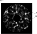
- FIG 2 illustrates in a simplified manner the formation of an image I of speckles.
- the light rays R which come from a star E (celestial object at infinity) form a plane wave O.
- the wave O' is disturbed.
- the image I obtained from its pupil has speckles S induced by the disturbed wave O'.
- the image I is acquired by means of an optical sensor 12 which is typically a CCD (Charged Coupled Device) or CMOS (Complementary Metal Oxide Semiconductor) sensor comprising an arrangement of pixels.
- the sensor 12 is defocused, that is to say positioned at a distance z (>0) from the focal plane Pf of said telescope.
- C n 2 is the structure constant of the refractive index of air (" refractive structure parameter" in English), measured in m -2/3 .
- refractive structure parameter is the structure constant of the refractive index of air
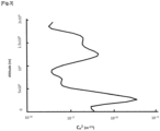
- This parameter expresses the intensity of the optical contribution of atmospheric turbulence. Varying with altitude h, it is generally noted C n 2 (h).
- the figure 3 illustrates an example of a C n 2 (h) profile.
- the MASS method for the acronym for Multiple Aperture Scintillation Sensor
- the SLODAR method for the acronym for SLOpe Detection And Ranging
- the SCIDAR method for the acronym for SCintillation Detection And Ranging
- the generalized SCIDAR method G-SCIDAR
- the Stereo-SCIDAR method [9]
- the PML method for the acronym for Profiler of Moon Limb
- the LuSci method for the acronym for Lunar Scintillometer
- CO-SLIDAR method for the English acronym of COupled SLope and Scintillation Detection And Ranging [12]
- the FASS method for the English acronym of Full Aperture Seeing Sensor
- the Fried parameter denoted r0.
- This parameter represents the spatial coherence width of the wave front.
- the parameter r0 can be expressed as a function of C n 2 (h) [15] and can therefore be deduced from the analysis of speckle images.
- the wind profile V(h) (where V characterizes the wind speed and direction and h the altitude) is another parameter for characterizing atmospheric turbulence and which can be deduced from the analysis of speckle images [16, 17].
- the disadvantages related to the methods of estimating the profile C n 2 (h) from speckle images are the same for estimating the parameter r0 or the wind profile V(h).
- Patent documents CN110083977 , US2019/277758 And US2012/078517 disclose other techniques used to characterize atmospheric turbulence.
- An objective of the invention is to remedy all or part of the aforementioned drawbacks.
- An additional objective of the invention is to be able to estimate simply, quickly and at low cost, at least one characteristic parameter of atmospheric turbulence.
- Another objective of the invention is to obtain a robust, reliable and precise method for interpreting images of optical speckles acquired in real observation conditions, in order to deduce one or more characteristic parameters of atmospheric turbulence.
- Yet another objective of the invention is to be able to estimate a characteristic parameter of atmospheric turbulence, without having to use dedicated complex instrumentation, but on the contrary being able to use an amateur telescope not dedicated to this type of analysis.
- This estimation method is now based on a machine learning model and therefore on an artificial intelligence model.
- the learning model is capable of automatically estimating a characteristic parameter of atmospheric turbulence, in particular a profile C n 2 (h), a Field parameter r0, or a wind profile V(h).
- the invention even makes it possible to estimate several parameters simultaneously if the learning model is trained with several characteristic parameters as training data.
- the trained learning model can be easily implemented at low cost in an amateur telescope, without the need to use specifically dedicated instrumentation.
- the use of a machine learning model makes it possible to overcome the mathematical models of the prior art, which are generally based on assumptions, considerations, approximations and/or negligibilities that negatively impact the calculations used to estimate the characteristic parameters. The invention therefore makes it possible to improve the estimation of a characteristic parameter studied.
- the method and system which are the subject of the invention are capable of generating manipulations of physical elements, in particular (electrical) signals and digital data, capable of being stored, transferred, combined, compared, etc., and making it possible to achieve a desired result.
- the invention implements one or more computer applications executed by computer equipment.
- an equipment does something means “the computer application executed by a processing unit of the equipment does something”.
- the computer application does something means “the computer application executed by the processing unit of the equipment does something”.
- the present invention may refer to one or more "computer processes”.
- the latter correspond to the actions or results obtained by the execution of instructions of one or more computer applications.
- "a computer process is adapted to do something” means "the instructions of a computer application executed by a processing unit do something”.
- the method which is the subject of the invention is based on the use of a machine learning model which is trained so as to estimate at least one characteristic parameter of atmospheric turbulence from images of optical speckles acquired in real conditions by a telescope (hereinafter referred to as "measuring telescope").
- the characteristic parameters that can be estimated include: a profile C n 2 (h); a Fiel parameter r0; a wind profile V(h).
- Other characteristic parameters can be estimated by the trained machine learning model. To do this, simply use as training data of optical speckle images associated with another desired characteristic parameter.
- optical speckle images used as training data correspond to real or simulated defocused images of one or more stars.
- the speckle images used as training data are images acquired in real conditions by an optical instrument, in particular a telescope, hereinafter referred to as a “training telescope”. These real images are defocused images of one or more stars.
- This training telescope may be an instrument dedicated to the acquisition of speckle images. It may be the same telescope as the measuring telescope or a different telescope.
- the training telescope is an amateur or consumer telescope, i.e. commercially available and not dedicated to the acquisition of speckle images.
- a smart telescope marketed by the company Unistellar ® under the reference eVscope ® .
- the values of the characteristic parameter(s) associated with these real images acquired by the training telescope can be estimated by one or more of the aforementioned known methods: MASS, SLODAR, SCIDAR, G-SCIDAR, Stereo-SCIDAR, PML, LuSci, CO-SLIDAR, FASS, DIMM (Differential Image Motion Monitor) [26, 27], etc.
- the values of the characteristic parameters can also be measured in reality, for example using sensors installed in atmospheric balloons, as described in [18] or [19]. It is then sufficient to correlate the values actually measured with the speckle images acquired during the measurement campaign.
- the speckle images used as training data are simulated images corresponding to defocused images of one or more stars. These speckle images are simulated - or modeled - from a characteristic parameter, for example from a profile C n 2 (h), a Fried parameter r0, a wind profile V(h).
- a characteristic parameter for example from a profile C n 2 (h), a Fried parameter r0, a wind profile V(h).
- Such Scintillation screen simulations are described in particular in [20, 21, 22, 23, 24].
- the general principle of these simulations is as follows: at a given altitude h, the effect of the atmosphere on the light wave is calculated. This effect generally only concerns the phase of the wave. Using Kolmogorov or Van Karman turbulence models, this effect is taken into account by calculating "phase screens".
- this disturbed wave is then calculated (for example by decomposition into plane waves, by Fresnel diffraction, ...), typically between the altitude where the phase disturbance was induced, and the ground. Under the effect of this propagation, the phase disturbances gradually transform into amplitude disturbance of the wave (scintillation effect).
- Numerical implementations of these calculation methods are for example described in [22, 23]. These calculations can be optimized by taking into account the phase perturbations induced at different altitudes. There are also open source Python libraries capable of doing these calculations, for example the AOtools library [25].
- the simulation algorithm used to model speckle images is parameterized according to the characteristics of the measuring telescope that will be used for acquiring speckle images in real conditions and that will be used as input data for the trained learning model.
- the simulation algorithm is developed by taking into account as parameters in particular: the focal length of the measuring telescope and/or its resolution (pixel size of the optical sensor) and/or the size of the acquired image (number of pixels of the optical sensor) and/or the shape of its pupil (for example: the presence of a mechanical structure at the entrance of the tube).
- the simulated images used as learning data are similar to the real images that will be acquired by the measuring telescope.
- the speckle images are simulated by placing themselves in real measurement conditions.
- the learning model is therefore more robust, more reliable and more precise.
- the simulated images used as training data are refined or corrected by real images acquired by the training telescope and which correspond to the same parameters. characteristics, for example to the same profile C n 2 (h), the same Fiel parameter r0, the same wind profile V(h).
- speckle images are advantageously simulated with varying intensities. These intensity variations correspond to the different intensities of the stars likely to be observed by the measuring telescope. This avoids the measuring telescope being forced to generate one or more speckle images by observing a predetermined star in real conditions.
- the trained learning model can instead accept as input data one or more speckle images from any star.
- Machine learning is based on an artificial intelligence model.
- the training database (or training set) is the set of pairs consisting of the values of the characteristic parameters associated with the speckle images.
- the learning model used is in this sense a supervised model.
- the model uses this learning base to develop a prediction function that makes it possible to associate a new input (i.e. one or more speckle images) with an output (i.e. a profile C n 2 (h) and/or a Fried parameter r0 and/or a wind profile V(h), .
- the learning model is based on an artificial neural network, on a Bayesian model, on a k-nearest neighbors (k-NN) algorithm, on a hidden Markov model, and more generally on a model which accepts the speckle image as input, and which generates as output values of one or more parameters characteristic of atmospheric turbulence such as a profile C n 2 (h), a Fried parameter r0, a wind profile V(h), or any other parameter characteristic of atmospheric turbulence.
- k-NN k-nearest neighbors
- FIGS. 4A to 4D illustrate different learning - or training - modes of the ML machine learning model.
- These training modes are exemplified by taking as a characteristic parameter of atmospheric turbulence a profile C n 2 (h).
- the person skilled in the art will understand easily that these training modes can be implemented with another characteristic parameter such as a Fried parameter r0 or a wind profile V(h).
- These training modes can also be implemented with several characteristic parameters.
- the speckle image(s) used as training data are simultaneously associated with a profile C n 2 (h) and a Fried parameter r0 and/or a wind profile V(h).
- C n 2 (h) profiles are used as training data, each profile being associated with one or more speckle images.
- several values of the same characteristic parameter i.e. several C n 2 (h) profiles
- each value i.e. each C n 2 (h) profile
- the speckle image(s) used as training data are real images or simulated images as explained previously.
- the training of the MLa model is carried out by associating a single image I(z) with each profile C n 2 (h).
- the image I(z) is a real acquired image or a simulated image in a single defocus plane z.
- the choice of this defocus plane z can be defined according to the method described in [14].
- the training database is here formed of a plurality of pairs ⁇ C n 2 (h)-I(z) ⁇ , for example between 500 and 10 6 pairs.
- the training of the MLb model is carried out by associating a series of images I(zi) with each profile C n 2 (h).
- the images I(zi) are here acquired actually or simulated in several defocus planes zi (i varying from -I to +k with for example I and k between 0 mm and 3 mm).
- defocus plane zi we therefore have a speckle image.
- the number of defocus planes zi can be between 2 and 1000.
- the different zi planes can be located in front and/or behind the focal plane Pf.
- the training database is here formed of a plurality of pairs ⁇ C n 2 (h)-I(zi) ⁇ , for example between 500 and 10 6 pairs.
- the training of the MLb model is more efficient than the Mla model and makes it possible to obtain a better estimate once the MLb model has been trained.
- the training of the MLb model is carried out by associating a series of images I(z, tj) with each profile C n 2 (h).
- the images I(z, tj) are acquired actually or simulated in a single defocus plane z as previously described with reference to the model of the Figure 4A , but over an acquisition period tj.
- the learning is thus also based on an analysis of the scintillation effect of speckles.
- the number of images I(z, tj) acquired or simulated over this period tj can for example be between 10 and 30,000.
- the learning database is therefore here formed of a plurality of pairs ⁇ C n 2 (h)-I(z,tj) ⁇ , for example between 500 and 10 6 pairs.
- the learning of the MLc model is more efficient than the Mla model and makes it possible to obtain a better estimate once the MLc model has been trained.
- the method of realization of the figure 4D is a combination of the modes of Figures 4B And 4C .
- the training of the MLd model is carried out by associating several series of images I(zi, tj) with each profile C n 2 (h).
- the images I(zi, tj) are here acquired actually or simulated in several defocus planes zi (as for the model of the Figure 4B ) and, for each defocusing plane zi, over an acquisition period tj (as for the model of the Figure 4C ).
- the training database is here formed of a plurality of pairs ⁇ C n 2 (h)-I(zi,tj) ⁇ , for example between 500 and 10 6 pairs.
- the training of the MLd model is more efficient than the Mla, MLb and Mlc models and allows to obtain a better estimate once the MLd model is trained.
- the training of the ML model can be based on the implementation mode of the Figure 4A and/or depending on the method of carrying out the Figure 4B and/or depending on the method of carrying out the Figure 4C and/or depending on the method of carrying out the figure 4D .
- the training of the ML model is carried out by a processing unit, preferably a computer server.
- the application based on this model is then implemented later in a memory area of a user telescope, for example by downloading.
- This computer application can then be enriched, for example by updates and/or downloads from remote databases in a computer server.
- a measuring telescope is used to acquire speckle images corresponding to defocused images of one or more stars observed in real conditions. These images can be acquired by orienting the measuring telescope at the zenith or by orienting said telescope between the horizon and the zenith, by adjusting its declination axis. These speckle images are the input data of the trained learning model.
- the measuring telescope used is an instrument dedicated to the acquisition of speckles.
- the telescope 1 is an amateur or general public telescope, i.e. commercially available and not dedicated to the analysis of a parameter characteristic of atmospheric turbulence.
- a smart telescope marketed by the company Unistellar ® under the reference eVscope ® .
- This is a telescope used for the observation of stars such as planets, comets, nebulae, galaxies, and generally celestial - or astronomical - objects near or far (in particular deep sky stars).
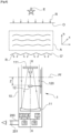
- the measuring telescope 1 comprises in particular a hollow body 10, an optical system 11 and a sensor 12.
- the hollow body 10 is for example in the form of a hollow tube of circular section, but could be a tube of oval, square, octagonal, or other section. It is specified that the hollow body 10 is not necessarily of tubular shape, but can be of conical shape, or formed of portions of tubes or cones for example.
- the hollow body 10 can be made of metal, plastic material, composite material, etc. For example, its length is between 200 mm and 1000 mm, its diameter is between 50 mm and 500 mm and its thickness is between 1 mm and 10 mm.
- the light rays R coming from an observed star E enter the tube 10 and are then reflected by a primary mirror 11, which is advantageously in the form of a concave parabolic mirror with pure reflection.
- the light rays R reflected by the mirror 11 form, in a focal plane Pf, an image of the star E.
- the sensor 12 is centered on the optical axis X-X and placed at a distance from the focal plane Pf so as to acquire the image of the pupil of the telescope 1, that is to say the image of the entrance end 100 of the tube 10.
- This image is the speckle image from which we seek to extract the values of the characteristic parameter(s) of atmospheric turbulence.
- the position of the sensor 12 is denoted z. This is the defocusing plane.
- the sensor 12 is movable so as to vary its position z. It is for example mounted mobile in translation on a longitudinal slide 120.
- the sensor 12 remains fixed and the configuration of the optical system is varied, in particular by moving the primary mirror 11, to vary the position of the focal plane Pf.
- the sensor 12 is positioned in the focal plane Pf for conventional use of the telescope 1 (i.e. for observing stars) and offset from said focal plane for implementing the method according to the invention. These positions z may be located in front of the focal plane Pf, i.e. between said focal plane and the mirror 11 and/or located behind said focal plane, i.e. between said focal plane and the input end 100.
- the sensor 12 is preferably a CCD (Charged Coupled Device) or CMOS (Complementary Metal Oxide Semiconductor) sensor comprising an arrangement of pixels (preferably generating color images). This type of sensor 12 has reduced dimensions, which allows it to be easily installed in the tube 10, while maintaining optimal brightness.
- the diameter of the sensor 12 is for example between 15 mm and 30 mm.
- the image data generated by the sensor 12 are transmitted to a processing unit 13.
- the connection between the sensor 12 and the processing unit 13 can be made in a wired manner, or by a wireless link, for example according to a proximity communication protocol, such as, by way of non-limiting example, the Bluetooth® , Wifi® , ZigBee® protocol.
- the processing unit 13 is adapted to use the images acquired by the sensor 12 as input data for the trained learning model.
- the processing unit 13 is adapted to transmit the images acquired by the sensor 12 to a remote computer server in which the trained learning model is implemented, which images are the input data for said model.
- the measuring telescope 1 also comprises one or more of the following computing resources: one or more memories 14, a wireless communication module 15, a network interface 16.
- the memory(ies) 14 must be considered as a storage device also suitable for storing data and/or data files. It may be a native memory or an attached memory such as a Secure Digital (SD) card.
- SD Secure Digital
- the trained learning model is preferably stored in this memory area 14.
- One or more other computer applications may also be stored in the memory area 14 and whose instructions, when executed by the processing unit 13, make it possible to perform functionalities described further in the description.
- the wireless communication module 15 is adapted to receive and transmit radio frequency signals to communicate wirelessly with other equipment.
- These radio frequency signals are preferably signals using a Bluetooth ® protocol, other protocols such as ISM, Wifi ® , ANT, ZIGBEE ® or other, may however be used.
- the network interface 16 is adapted to establish communication between the telescope 1 and a remote computer server and/or other remote electronic equipment, via a computer communication network.
- This network interface 16 can be directly integrated into the telescope 10 and is present for example in the form of a GSM module (for the English acronym Global System for Mobile Communication), allowing it to connect to a mobile telephone communication network.
- GSM Global System for Mobile Communication
- the measuring telescope 1 can also advantageously integrate a rechargeable electric power supply battery 17, so as to make said telescope completely autonomous.
- the measuring telescope 1 integrates a viewing device formed by one (or two) eyepieces 200 provided with a viewing screen 201, for example a polychrome liquid crystal screen LCD (for Liquid Crystal Display) or OLED (for Organic Light-Emitting Diode).
- the processing unit 13 is adapted to display the images acquired by the sensor 12 on the screen 101.
- the screen 201 is integrated into a display device that is remote from the telescope 1.
- a display device that is remote from the telescope 1.
- This is for example a head-mounted display (also called a display headset, immersive headset, screen headset or HMD headset for the English acronym for head-mounted display) of the type described in the patent document EP3400474 (GOOGLE) or a screen of a mobile terminal, for example the screen of a Smartphone (smart phone) or a touch pad.
- a head-mounted display also called a display headset, immersive headset, screen headset or HMD headset for the English acronym for head-mounted display
- a screen of a mobile terminal for example the screen of a Smartphone (smart phone) or a touch pad.
- connection between this remote viewing device and the telescope 1, and more particularly with the processing unit 13, can be made via a wired connection (for example by means of a USB cable) or via a wireless connection, for example according to a proximity communication protocol, such as, by way of non-limiting example, the Bluetooth ® , Wifi ® , ZigBee ® protocol.
- a proximity communication protocol such as, by way of non-limiting example, the Bluetooth ® , Wifi ® , ZigBee ® protocol.
- the primary mirror 110 and secondary mirror 111 are positioned on the same optical axis XX. They are arranged so that the light rays reflected by said mirrors form, in the focal plane Pf, an image of the observed star.
- the mirrors 110, 111 are arranged so that the focal plane Pf is located in the tube 10, between the two said mirrors.
- the primary mirror 110 is preferably a concave parabolic mirror having a low focal ratio (preferably less than 5). This type of mirror makes it possible to overcome spherical aberrations.
- the diameter of the primary mirror 110 corresponds substantially to the diameter of the tube 10.
- the position of the sensor 12 is denoted z.
- the sensor 12 can be placed in different defocusing positions z located on either side of the focal plane Pf. These positions can be located in front of the focal plane Pf, i.e. between said focal plane and the primary mirror 110 and/or located behind said focal plane, i.e. between said focal plane and the secondary mirror 111.
- the sensor 12 can be mounted mobile in translation on a longitudinal slide 120 to vary its position z.
- the sensor 12 remains fixed and the configuration of the optical system is varied, in particular by moving the primary mirror 110 and/or the secondary mirror 111, to vary the position of the focal plane Pf.
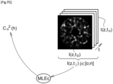
- FIGS. 7A to 7C illustrate different modes of use of the trained learning model MLE.
- the trained learning model makes it possible to estimate one or more characteristic parameters from an input data containing one or more images of optical speckles acquired by the measuring telescope 1. These speckle images are defocused images of one or more stars observed in real conditions by the measuring telescope 1.
- the trained MLE learning model can be implemented directly in the measuring telescope 1, or be implemented in a remote computer server.
- a characteristic parameter to be estimated a profile C n 2 (h).
- these modes of use are also suitable for estimating one or more other characteristic parameters such as a Fried parameter r0, a wind profile V(h), etc.
- the trained learning model can therefore provide several output data, each corresponding to values of a specific characteristic parameter, for example: a profile C n 2 (h) and a Fried parameter r0 and a wind profile V(h).
- the input data consists of a single speckle image I(z) actually acquired by the sensor 12.
- This speckle image I is the input data of the trained learning model MLEa.
- the output data is the desired characteristic parameter, here a profile C n 2 (h).
- the trained learning model MLEa is the MLa model trained according to the embodiment of the Figure 4A .
- the input data (a single speckle image) thus corresponds to the type of training data, so that the estimation of the profile C n 2 (h) is optimized.
- the estimation of the profile C n 2 (h) is all the more precise when the MLa training model is trained with simulated speckle images, and the simulation algorithm used is parameterized according to the characteristics of the measuring telescope 1.
- the real image I is acquired in a single defocus plane z. In order to optimize the estimation of the profile C n 2 (h), this defocus plane corresponds to that in which the images used as training data for the MLa model were simulated.
- the MLa model ( Figure 4A ) can also be trained with speckle images actually acquired by the training telescope. If the measuring telescope 1 is the training telescope, it is sufficient to place the sensor 12 in the same defocusing plane z as that used to acquire the images training. In other words, the same z-defocus plane is used for the acquisition of the speckle images used as training data for the MLa model and for the acquisition of the speckle image used as input data for the trained MLEa model.
- the measuring telescope 1 is different from the training telescope (in particular with regard to its focal length and/or its resolution and/or its acquired image size and/or its pupil shape), it is advantageous to provide specific processing to adapt the measurement conditions to the learning conditions so that the input data of the trained model MLEa are equivalent to the learning data of the model MLa.
- the estimation of the trained learning model MLEa is then more precise and more reliable.
- the measuring telescope 1 has a focal length (f measurement ) different from the focal length (f drive ) of the training telescope, it is appropriate to adapt the defocus (z measurement ) of the sensor 12 of said measuring telescope so that it is equivalent to the defocus (z drive ) of the sensor of said training telescope.
- the measuring and training telescopes may not have the same resolution, the size of the pixels of their respective optical sensor being different. It is advantageous in this case to adapt the resolution of the sensor 12 of the measuring telescope 1 so that it is equivalent to that of the training telescope.
- This adaptation can for example be carried out according to an image processing algorithm of the type described in [28] or [29], or according to image processing software proposed by the company Let's Enhance ® (https://letsenhance.io). This adaptation is advantageously carried out by the processing unit 13.
- the size of the measurement image acquired (number of pixels of the optical sensor) by the measurement telescope 1 may be different from the size of the training image acquired by the training telescope. It is then advantageous to adapt the size of the measurement image so that it is equivalent to that of the training image.
- This resizing can consist of scaling, cropping, vectorization, resizing of the type based on cubic interpolation [30], linear interpolation [31] or non-linear interpolation (for example described in US6727908 ), a nearest neighbor interpolation [32], etc.
- This adaptation is advantageously carried out by the processing unit 13.
- the measuring and training telescopes may not have the same pupil shape.
- the training telescope may have a structure at the tube entrance supporting a secondary mirror or an optical sensor, and whose shape is different from that of the measuring telescope 1.
- the shape of such a structure is visible on the speckle images. It is therefore advantageous to provide image processing so that the shape of the structure appearing on the measuring image is equivalent to that appearing on the training image.
- a mask reproducing the shape of the structure at the input of the training telescope can be added to the measurement image.
- the input data consists of a series of speckle images I(zi) actually acquired by the sensor 12.
- This series of images is the input data of the trained learning model MLEb.
- the output data is the characteristic parameter sought, here a profile C n 2 (h).
- the images I(zi) are acquired in several defocus planes zi (i varying from -I to +k with for example I and k between 0 mm and 3 mm). For each defocus plane zi, we therefore have a speckle image.
- the number of defocus planes zi can be between 2 and 1000.
- the different planes zi can be located in front of and/or behind the focal plane Pf.
- the trained learning model MLEb is the MLb model ( Figure 4B ).
- the input data (a series of speckle images) thus corresponds to the type of training data, so that the estimation of the profile C n 2 (h) is optimized.
- the estimation of the profile C n 2 (h) is all the more accurate when the MLb learning model is trained with simulated speckle images, and the simulation algorithm used is parameterized according to the characteristics of the measuring telescope 1.
- the real images I(zi) are acquired in several defocus planes zi. In order to optimize the estimation of the profile C n 2 (h), these defocus planes correspond to those in which the images used as training data for the MLd model were simulated.
- the MLb model ( Figure 4B ) can also be trained with speckle images actually acquired by the training telescope. If the measuring telescope 1 is the training telescope, it is sufficient to place the sensor 12 in the same defocus planes zi as those used to acquire the training images. The same defocus planes zi are therefore used for the acquisition of the training images of the MLb model and for the acquisition of the measurement images used as input data for the trained model MLEb.
- the measuring telescope 1 is different from the training telescope (in particular as regards its focal length and/or its resolution and/or its acquired image size and/or its pupil shape)
- a specific image processing is advantageously provided to adapt the measurement conditions to the learning conditions so that the input data of the trained model MLEb are equivalent to the learning data of the model MLb.
- the image processing concerning the adaptation of the defocusing, the adaptation of the resolution, the adaptation of the image size and/or the adaptation of the pupil image are similar to those described with reference to the Figure 7A .
- the input data consists of a series of images I(z, tj) of speckles actually acquired by the sensor 12.
- This series of images is the input data of the trained learning model MLEc.
- the output data is the characteristic parameter sought, here a profile C n 2 (h).
- the number of images I(z, tj) acquired over this period tj can for example be between 10 and 30,000.
- the trained learning model MLEc is the MLc model ( Figure 4C ).
- the input data (a series of speckle images) thus corresponds to the type of training data, so that the estimation of the profile C n 2 (h) is optimized.
- the estimation of the profile C n 2 (h) is all the more precise when the learning model MLc is trained with simulated speckle images, and the simulation algorithm used is parameterized according to the characteristics of the measuring telescope 1.
- the real images I(z, tj) are acquired in a single defocus plane z. In order to optimize the estimation of the profile C n 2 (h), this defocus plane corresponds to the one in which the images used as training data for the model MLb were simulated.
- the MLc model ( Figure 4C ) can also be trained with speckle images actually acquired by the training telescope. If the measuring telescope 1 is the training telescope, it is sufficient to place the sensor 12 in the same defocus plane z as that used to acquire the training images and to acquire the measurement images over the same period tj. The same defocus plane z and the same acquisition period are therefore used for the acquisition of the training images of the MLc model and for the acquisition of the measurement images used as input data for the trained model MLEc.
- the measuring telescope 1 is different from the training telescope (in particular as regards its focal length and/or its resolution and/or its acquired image size and/or its pupil shape)
- a specific image processing is advantageously provided to adapt the measurement conditions to the learning conditions so that the input data of the trained model MLEc are equivalent to the learning data of the model MLc.
- the image processing concerning the adaptation of the defocusing, the adaptation of the resolution, the adaptation of the image size and/or adaptation of the pupil image are similar to those described with reference to the Figure 7A .
- the method of realization of the Figure 7D is a combination of the modes of Figures 7B And 7C .
- the input data consists of several series of images I(zi, tj) of speckles actually acquired by the sensor 12. All of these series of images are the input data of the trained learning model MLEd.
- the output data is the desired characteristic parameter, here a profile C n 2 (h).
- the images I(zi, tj) are acquired in several defocusing planes zi (as for the model of the Figure 7B ) and over an acquisition period tj (as for the model of the Figure 7C ).
- the trained learning model MLEd is the MLd model ( figure 4D ).
- the input data severe series of speckle images
- the estimation of the profile C n 2 (h) is all the more precise when the training model MLd is trained with simulated speckle images, and the simulation algorithm used is parameterized according to the characteristics of the measuring telescope 1.
- the real images I(zi, tj) are acquired in several defocus planes zi. In order to optimize the estimation of the profile C n 2 (h), these defocus planes correspond to those in which the images used as training data for the MLd model were simulated.
- the MLd model ( figure 4D ) can also be trained with speckle images actually acquired by the training telescope. If the measuring telescope 1 is the training telescope, it is sufficient to place the sensor 12 in the same defocus planes zi as those used to acquire the training images and to acquire the measurement images over the same period tj. The same defocus planes zi and the same acquisition period are therefore used for the acquisition of the training images of the MLd model and for the acquisition of the measurement images used as input data for the trained model MLEd.
- the measuring telescope 1 is different from the training telescope (in particular with regard to its focal length and/or its resolution and/or its acquired image size and/or its pupil shape)
- a specific image processing is advantageously provided to adapt the measurement conditions to the learning conditions so that the input data of the trained model MLEd are equivalent to the learning data of the model MLd.
- the image processing concerning the adaptation of the defocusing, the adaptation of the resolution, the adaptation of the image size and/or the adaptation of the pupil image are similar to those described with reference to the Figure 7A .
- a single measuring telescope 1 makes it possible to acquire speckle images as a function of defocusing positions z which make it possible to estimate a characteristic parameter of atmospheric turbulence according to altitude h, in particular a profile C n 2 (h) or a wind profile V(h).
- atmospheric turbulence is not only inhomogeneous according to altitude h, but also according to longitude (x axis on the figures 2 , 5 And 6 ) and latitude (y axis on the figures 2 , 5 And 6 ).
- one solution is to carry out measurements according to the methods explained above and by varying the declination axis and/or the ascension axis between each measurement.
- speckle images which do not depend only on the defocus z and possibly on the time t - I(z,t) - but also on the longitude and latitude - I(x,y,z,t). This series of measurements can however prove tedious.
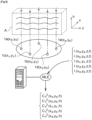
- FIG. 8 An alternative solution is shown schematically in the figure 8 .
- Several measuring telescopes 1a, 1b, 1c, 1d, 1e are arranged in a network. For example, between 5 and 1000 measuring telescopes are networked. These telescopes 1a, 1b, 1c, 1d, 1e are installed so as to mesh a specific geographical area Geo, for example a city or an observation site.
- Each telescope 1a, 1b, 1c, 1d, 1e has its own longitude and latitude position, respectively x a -y a , x b -y b , x c -y c , x d -y d , x e -y e .
- Each telescope 1a, 1b, 1c, 1d, 1e acquires one or more speckle images as explained above (i.e. in one or more defocusing planes and/or over an acquisition time period) which also depend on the longitude and latitude of said telescope.
- These images are respectively referenced I(x a -y a ,z,t), I(x b -y b ,z,t), I(x c -y c ,z,t), I(x d -y d ,z,t), I(x e -y e ,z,t) on the figure 8 .
- the images I(x a -y a ,z,t), I(x b -y b ,z,t), I(x c -y c ,z,t), I(x d -y d ,z,t), I(x e -y e ,z,t) are transmitted to a remote computer server Serv in which the trained learning model MLE is implemented.
- the communication between the telescopes 1a, 1b, 1c, 1d, 1e can be done through a communication network, for example by means of a network interface integrated in each of the telescopes of the network 1a, 1b, 1c, 1d, 1e.
- the images I(x a -y a ,z,t), I(x b -y b ,z,t), I(x c -y c ,z,t), I(x d -y d ,z,t), I(x e -y e ,z,t) are transmitted to a "master" measuring telescope, for example the telescope 1a, in which the trained learning model MLE is implemented.
- the communication between the "slave" telescopes 1b, 1c, 1d, 1e and the "master” telescope 1a can here again be done via a communication network, for example by means of a network interface integrated in each of the telescopes of the network 1a, 1b, 1c, 1d, 1e.
- the images I(x a -y a ,z,t), I(x b -y b ,z,t), I(x c -y c ,z,t), I(x d -y d ,z,t), I(x e -y e ,z,t) are the input data of the trained MLE model.
- the MLE model is then able to estimate a characteristic parameter, for example a profile C n 2 (h) at different longitudes and latitudes, respectively C n 2 (x a -y a ,h), C n 2 (x b -y b ,h), C n 2 (x c -y c ,h), C n 2 (x d -y d ,h), C n 2 (x e -y a ,h).
- a characteristic parameter for example a profile C n 2 (h) at different longitudes and latitudes, respectively C n 2 (x a -y a ,h), C n 2 (x b -y b ,h), C n 2 (x c -y c ,h), C n 2 (x d -y d ,h), C n 2 (x e -y a ,h).
- This characterization of turbulence in altitude, longitude and latitude is particularly useful. In particular, it can be used to detect the best area to install an observation site. It can also be used to detect an inversion layer formed above a city and anticipate measures to reduce pollution (for example, alternating traffic). It should be noted here that an inversion layer is a layer of air with a positive temperature gradient. This inversion layer behaves like a "bell" that traps pollution, particularly that caused by road traffic or smoke from industrial chimneys.
- This inversion layer can be deduced from the profiles C n 2 (x a -y a ,h), C n 2 (x b -y b ,h), C n 2 (x c -y c ,h), C n 2 (x d -y d ,h), C n 2 (x e -y e ,h).
- one or more features disclosed only in one embodiment may be combined with one or more other features disclosed only in another embodiment.
- one or more features disclosed only in one embodiment may be generalized to other embodiments, even if that feature or features are described only in combination with other features.
Landscapes
- Engineering & Computer Science (AREA)
- Environmental & Geological Engineering (AREA)
- Theoretical Computer Science (AREA)
- Life Sciences & Earth Sciences (AREA)
- Atmospheric Sciences (AREA)
- Biodiversity & Conservation Biology (AREA)
- Ecology (AREA)
- Environmental Sciences (AREA)
- Evolutionary Computation (AREA)
- Software Systems (AREA)
- Computing Systems (AREA)
- Databases & Information Systems (AREA)
- Artificial Intelligence (AREA)
- General Health & Medical Sciences (AREA)
- Medical Informatics (AREA)
- Computer Vision & Pattern Recognition (AREA)
- Health & Medical Sciences (AREA)
- Physics & Mathematics (AREA)
- General Physics & Mathematics (AREA)
- Multimedia (AREA)
- Image Processing (AREA)
- Image Analysis (AREA)
- Management, Administration, Business Operations System, And Electronic Commerce (AREA)
- Optical Radar Systems And Details Thereof (AREA)
Claims (17)
- Verfahren zum Schätzen eines charakteristischen Parameters der atmosphärischen Turbulenz, wobei das Verfahren die Schritte beinhaltet, bestehend aus:- Trainieren eines automatischen Lernmodells unter Verwendung der Werte des charakteristischen Parameters, denen Bilder von optischen Flecken zugeordnet sind, als Lerndaten,- Verwenden des trainierten Lernmodells, um den charakteristischen Parameter aus einem Eingabedatum zu schätzen, das ein oder mehrere Bilder von optischen Flecken enthält,dadurch gekennzeichnet, dass- die Bilder von optischen Flecken, die beim Trainieren des Lernmodells verwendet werden, unscharfen Bildern eines oder mehrerer Sterne entsprechen,- das oder die Bilder von optischen Flecken, die in dem Eingabedatum enthalten sind, durch mindestens ein Messteleskop (1) erfasst werden, wobei die Fleckenbilder unscharfen Bildern eines oder mehrerer Sterne entsprechen, die unter reellen Bedingungen von dem Teleskop beobachtet worden sind.
- Verfahren nach Anspruch 1, bestehend aus:- Trainieren des automatischen Lernmodells unter Verwendung der Werte mehrerer charakteristischer Parameter der atmosphärischen Turbulenz, denen Bilder von optischen Flecken zugeordnet sind, die unscharfen Bildern eines oder mehrerer Sterne entsprechen, als Lerndaten,- Verwenden des trainierten Lernmodells, um jeden der charakteristischen Parameter aus einem Eingabedatum zu schätzen, welches ein oder mehrere Bilder von optischen Flecken enthält, die von dem Messteleskop (1) erfasst werden.
- Verfahren nach einem der Ansprüche 1 oder 2, wobei der oder die charakteristischen Parameter einer atmosphärischen Turbulenz aus der folgenden Liste ausgewählt werden: einem Profil Cn 2(h) wobei Cn 2 die Strukturkonstante des Brechungsindex der Luft ist, und h die Höhe ist; einem Fried-Parameter r0; einem Profil des Windes V(h) wobei V die Richtung und die Geschwindigkeit des Windes, und h die Höhe charakterisieren.
- Verfahren nach einem der Ansprüche 1 bis 3, das darin besteht, das Lernmodell (MLa) unter Verwendung der Werte eines charakteristischen Parameters einer atmosphärischen Turbulenz als Lerndaten zu trainieren, wobei jeder Wert einem tatsächlich erfassten oder simulierten Bild von optischen Flecken in einer einzigen Defokussierungsebene (z) zugeordnet ist.
- Verfahren nach Anspruch 4, das darin besteht, ein Bild von Flecken, das in der Defokkussierungsebene (z) erfasst wurde, als Eingabedatum des trainierten Lernmodells (MLEa) zu verwenden.
- Verfahren nach einem der Ansprüche 1 bis 3, das darin besteht, das Lernmodell (MLb) unter Verwendung mehrerer Werte eines charakteristischen Parameters einer atmosphärischen Turbulenz als Lerndaten zu trainieren, wobei jeder Wert einer Reihe von tatsächlich erfassten oder simulierten Bildern von Flecken in mehreren Defokussierungsebenenen (zi) zugeordnet wird.
- Verfahren nach Anspruch 6, das darin besteht, eine Reihe von in den Defokussierungsebenen (zi) erfassten Bildern von Flecken als Eingabedatum des trainierten Lernmodells (MLEb) zu verwenden.
- Verfahren nach einem der Ansprüche 1 bis 3, das darin besteht, das Lernmodell (MLc) unter Verwendung mehrerer Werte eines charakteristischen Parameters einer atmosphärischen Turbulenz als Lerndaten zu trainieren, wobei jeder Wert einer Reihe von tatsächlich erfassten oder simulierten Bildern von Flecken in einer einzigen Defokussierungsebene (z) und über einen Erfassungszeitraum (tj) hinweg zugeordnet wird.
- Verfahren nach Anspruch 8, das darin besteht, eine Reihe von in der Defokussierungsebene (z) und über den Erfassungszeitraum (tj) hinweg erfassten Bildern von Flecken als Eingabedatum des trainierten Lernmodells (MLEc) zu verwenden.
- Verfahren nach einem der Ansprüche 1 bis 3, das darin besteht, das Lernmodell (MLd) unter Verwendung mehrerer Werte eines charakteristischen Parameters einer atmosphärischen Turbulenz als Lerndaten zu trainieren, wobei jeder Wert mehreren Reihen von tatsächlich erfassten oder simulierten Bildern von Flecken in mehreren Defokussierungsebenen (zi) und für jede Defokussierungsebene (zi) über einen Erfassungszeitraum (tj) hinweg zugeordnet wird.
- Verfahren nach Anspruch 10, das darin besteht, mehrere Reihen von in den Defokussierungsebenen (zi) und für jede Defokussierungsebene (zi) über den Erfassungszeitraum (tj) hinweg erfassten Bildern von Flecken als Eingabedatum des trainierten Lernmodells (MLEd) zu verwenden.
- Verfahren nach einem der Ansprüche 6, 7, 10, 11, wobei sich die verschiedenen Defokussierungsebenen (zi) beiderseits einer Brennebene (Pf) befinden.
- Verfahren nach einem der vorstehenden Ansprüche, die Schritte umfassend, die darin bestehen:- als Lerndaten Bilder von Flecken zu verwenden, die aus Werten eines charakteristischen Parameters simuliert werden, wobei die Simulation anhand eines Simulationsalgorithmus durchgeführt wird,- den Simulationsalgorithmus in Abhängigkeit von den Eigenschaften des Messteleskops (1) zu parametrieren.
- Verfahren nach Anspruch 12, das darin besteht, den Simulationsalgorithmus unter Berücksichtigung der Brennweite des Messteleskops (1), und/oder der Auflösung des Messteleskops und/oder der Größe des von dem Messteleskop erfassten Bildes und/oder der Form einer Pupille des Messteleskops zu parametrieren.
- Verfahren nach einem der Ansprüche 1 bis 12, das darin besteht, als Lerndaten zu verwenden:- Bilder von optischen Flecken, die durch mindestens ein Trainingsteleskop erfasst werden, wobei die Fleckenbilder durch unscharfe Bildern eines oder mehrerer Sterne gebildet sind, die unter reellen Bedingungen von dem Teleskop beobachtet worden sind,- Werte eines charakteristischen Parameters, die den Bildern zugeordnet sind, wobei jeder Wert tatsächlich gemessen und/oder durch Umsetzen eines oder mehrerer der folgenden Verfahren geschätzt wird: MASS, SLODAR, SCIDAR, G-SCIDAR, Stereo-SCIDAR, PML, LuSci, CO-SLIDAR, FASS, DIMM.
- Verfahren nach einem der vorstehenden Ansprüche, die Schritte umfassend, die darin bestehen:- in einem Netzwerk mehrere Messteleskope (1a, 1b, 1c, 1d, 1e) anzuordnen, wobei jedes Teleskop des Netzwerks eine ihm eigene Position in der Länge und in der Breite aufweist,- ein oder mehrere Bilder von optischen Flecken mit einem der Teleskope (1a, 1b, 1c, 1d, 1e) zu erfassen,- eine Einheit der erfassten Bilder als Eingabedaten des trainierten Lernmodells (MLE) zu verwenden, um den charakteristischen Parameter in Abhängigkeit von der Länge und der Breite zu schätzen.
- Installation zum Schätzen eines charakteristischen Parameters der atmosphärischen Turbulenz gemäß dem Verfahren nach einem der Ansprüche 1 bis 16, die beinhaltet:- eine Bearbeitungseinheit, die konfiguriert ist, um ein automatisches Lernmodell unter Verwendung der Werte des charakteristischen Parameters zu trainieren, denen Bilder von optischen Flecken zugeordnet sind, die unscharfen Bildern eines oder mehrerer Sterne entsprechen, als Lerndaten,- mindestens ein Messteleskop (1), das angepasst ist, um ein oder mehrere Bilder von optischen Flecken zu erfassen, die unscharfen Bildern eines oder mehrerer Sterne entsprechen, die unter reellen Bedingungen von dem Teleskop beobachtet worden sind,- eine Bearbeitungseinheit, die angepasst ist, um das trainierte Lernmodell zu verwenden, um den charakteristischen Parameter aus einem Eingabedatum zu schätzen, welches ein oder mehrere Bilder von optischen Flecken enthält, die von dem Messteleskop (1) erfasst werden.
Applications Claiming Priority (2)
| Application Number | Priority Date | Filing Date | Title |
|---|---|---|---|
| FR2006810A FR3112006B1 (fr) | 2020-06-29 | 2020-06-29 | Procédé et installation pour estimer un paramètre caractéristique de la turbulence atmosphérique |
| PCT/EP2021/067814 WO2022002917A1 (fr) | 2020-06-29 | 2021-06-29 | Procédé et installation pour estimer un paramètre caractéristique de la turbulence atmosphérique |
Publications (3)
| Publication Number | Publication Date |
|---|---|
| EP4172665A1 EP4172665A1 (de) | 2023-05-03 |
| EP4172665C0 EP4172665C0 (de) | 2024-12-04 |
| EP4172665B1 true EP4172665B1 (de) | 2024-12-04 |
Family
ID=73401604
Family Applications (1)
| Application Number | Title | Priority Date | Filing Date |
|---|---|---|---|
| EP21739603.5A Active EP4172665B1 (de) | 2020-06-29 | 2021-06-29 | Verfahren und system zur schätzung eines charakteristischen parameters der atmosphärischen turbulenz |
Country Status (5)
| Country | Link |
|---|---|
| US (1) | US12455398B2 (de) |
| EP (1) | EP4172665B1 (de) |
| JP (1) | JP2023531783A (de) |
| FR (1) | FR3112006B1 (de) |
| WO (1) | WO2022002917A1 (de) |
Families Citing this family (6)
| Publication number | Priority date | Publication date | Assignee | Title |
|---|---|---|---|---|
| CN114417742B (zh) * | 2022-04-01 | 2022-06-10 | 中国工程物理研究院流体物理研究所 | 一种激光大气闪烁指数预测方法及系统 |
| CN118033590B (zh) * | 2024-04-12 | 2024-06-28 | 南京信息工程大学 | 一种基于改进vit神经网络的短临降水预报方法 |
| CN118276191B (zh) * | 2024-06-03 | 2024-08-09 | 中国科学院云南天文台 | 一种集成化通用型全时段的大气光学湍流测量设备 |
| CN119086014B (zh) * | 2024-08-29 | 2025-09-12 | 中国科学院南京天文光学技术研究所 | 用于超高对比度成像仪测试的望远镜系统模拟方法和装置 |
| CN119023220B (zh) * | 2024-10-29 | 2025-02-07 | 中国科学院云南天文台 | 一种地平式太阳望远镜轴系之间同轴度的监测方法与系统 |
| CN120951885B (zh) * | 2025-10-14 | 2025-12-26 | 珠海翔翼航空技术有限公司 | 基于kan网络的垂直大气廓线细粒度处理方法、系统及设备 |
Family Cites Families (13)
| Publication number | Priority date | Publication date | Assignee | Title |
|---|---|---|---|---|
| US5384455A (en) * | 1993-04-12 | 1995-01-24 | Environmental Research Institute Of Michigan | Measurement-diverse speckle imaging |
| US6216540B1 (en) * | 1995-06-06 | 2001-04-17 | Robert S. Nelson | High resolution device and method for imaging concealed objects within an obscuring medium |
| US6727908B1 (en) | 2000-08-31 | 2004-04-27 | Micron Technology, Inc. | Non-linear interpolation scaling system for a graphics processing system and method for use thereof |
| US7531774B2 (en) * | 2006-06-05 | 2009-05-12 | General Dynamics Advanced Information Systems, Inc. | Measurement-diverse imaging and wavefront sensing with amplitude and phase estimation |
| US8874374B2 (en) * | 2010-09-28 | 2014-10-28 | Darek J. Bogucki | Optical turbulence sensor |
| CN102662178B (zh) * | 2012-05-03 | 2013-11-27 | 中国科学院长春光学精密机械与物理研究所 | 空间目标白天高分辨率光电成像探测系统 |
| US9305378B1 (en) * | 2014-12-17 | 2016-04-05 | The Boeing Company | Lenslet, beamwalk and tilt diversity for anisoplanatic imaging by large-aperture telescopes |
| US9983382B2 (en) * | 2015-01-12 | 2018-05-29 | The Boeing Company | Active aperture partitioning for an imaging system |
| EP3391108A1 (de) * | 2015-12-17 | 2018-10-24 | Universite d'Aix-Marseille (AMU) | Systeme und verfahren für hochauflösende bildgebung anhand eines glasfaserbündels |
| US20170289529A1 (en) | 2016-03-29 | 2017-10-05 | Google Inc. | Anaglyph head mounted display |
| KR102777976B1 (ko) * | 2017-03-31 | 2025-03-07 | 앤마리 힙슬레이 | 눈 레이저 수술 및 치료적 처치를 위한 시스템 및 방법 |
| US10942119B2 (en) * | 2018-03-09 | 2021-03-09 | United States Of America As Represented By The Secretary Of The Navy | Characterizing atmospheric turbulence using the covariance and temporal intensity fluctuations of an optical source |
| CN110083977B (zh) * | 2019-05-14 | 2023-06-06 | 南京大学 | 一种基于深度学习的大气湍流监测方法 |
-
2020
- 2020-06-29 FR FR2006810A patent/FR3112006B1/fr active Active
-
2021
- 2021-06-29 WO PCT/EP2021/067814 patent/WO2022002917A1/fr not_active Ceased
- 2021-06-29 US US18/003,586 patent/US12455398B2/en active Active
- 2021-06-29 EP EP21739603.5A patent/EP4172665B1/de active Active
- 2021-06-29 JP JP2022581322A patent/JP2023531783A/ja active Pending
Also Published As
| Publication number | Publication date |
|---|---|
| WO2022002917A1 (fr) | 2022-01-06 |
| JP2023531783A (ja) | 2023-07-25 |
| FR3112006B1 (fr) | 2022-07-22 |
| EP4172665A1 (de) | 2023-05-03 |
| EP4172665C0 (de) | 2024-12-04 |
| US20230258842A1 (en) | 2023-08-17 |
| US12455398B2 (en) | 2025-10-28 |
| FR3112006A1 (fr) | 2021-12-31 |
Similar Documents
| Publication | Publication Date | Title |
|---|---|---|
| EP4172665B1 (de) | Verfahren und system zur schätzung eines charakteristischen parameters der atmosphärischen turbulenz | |
| Liu et al. | Phasor field diffraction based reconstruction for fast non-line-of-sight imaging systems | |
| Nagel et al. | Nanosatellites applied to optical Earth observation: a review | |
| Ziad et al. | Comparison of measurements of the outer scale of turbulence by three different techniques | |
| CA3226364A1 (en) | Enhancing generative adversarial networks using combined inputs | |
| CA2805010C (fr) | Systeme de veille spatiale pour la surveillance de l'espace proche | |
| CA2804996C (fr) | Procede de realisation d'un systeme de veille spatiale pour la surveillance de l'espace proche | |
| Jia et al. | PSF–net: a nonparametric point-spread function model for ground-based optical telescopes | |
| FR3087538A1 (fr) | Procede d'observation d'un echantillon | |
| EP3199941A1 (de) | Beobachtungsverfahren einer probe mittels bildgebungssystem ohne linse | |
| Denoyelle | Theoretical and numerical analysis of super-resolution without grid | |
| EP2909671B1 (de) | Verfahren zum auslegen einer einzelpfad-kamera zur bestimmung der tiefenschärfe | |
| Desmars | Real-time reconstruction and prediction of ocean wave fields from remote optical measurements | |
| Goyens et al. | Improving the standard protocol for above-water reflectance measurements: 1. Estimating effective wind speed from angular variation<? TeX\break?> of sunglint | |
| Bialek et al. | DanceCam: atmospheric turbulence mitigation in wide-field astronomical images with short-exposure video streams | |
| Courtney-Barrer et al. | Empirical contrast model for high-contrast imaging A VLT/SPHERE case study | |
| Zhang et al. | Accurate broadband wavefront sensing for space telescopes via a compact neural network | |
| Douglas et al. | Shadow imaging of geosynchronous satellites: simulation, image reconstruction, and shadow prediction | |
| FR3143160A1 (fr) | Procédé de prévision d’une séquence d’images par intelligence artificielle et son architecture de réseau de neurones | |
| Guo et al. | Computational imaging towards next-generation optical observational astronomy | |
| EP3995991A2 (de) | Verfahren zur erfassung eines zellulären ereignisses | |
| Li et al. | The design of a method for recovering degraded images of atmospheric turbulence based on deep learning | |
| Kodama et al. | Deep-learning-based single-pixel telescope for simultaneous visible and near-infrared imaging with robustness to atmospheric seeing | |
| Song et al. | Deep optics framework utilizing a liquid crystal microlens array for dynamic wavefront sensing and correction in atmospheric turbulence | |
| Hénault | Signal-to-noise ratio of phase sensing telescope interferometers |
Legal Events
| Date | Code | Title | Description |
|---|---|---|---|
| STAA | Information on the status of an ep patent application or granted ep patent |
Free format text: STATUS: UNKNOWN |
|
| STAA | Information on the status of an ep patent application or granted ep patent |
Free format text: STATUS: THE INTERNATIONAL PUBLICATION HAS BEEN MADE |
|
| PUAI | Public reference made under article 153(3) epc to a published international application that has entered the european phase |
Free format text: ORIGINAL CODE: 0009012 |
|
| STAA | Information on the status of an ep patent application or granted ep patent |
Free format text: STATUS: REQUEST FOR EXAMINATION WAS MADE |
|
| 17P | Request for examination filed |
Effective date: 20230123 |
|
| AK | Designated contracting states |
Kind code of ref document: A1 Designated state(s): AL AT BE BG CH CY CZ DE DK EE ES FI FR GB GR HR HU IE IS IT LI LT LU LV MC MK MT NL NO PL PT RO RS SE SI SK SM TR |
|
| DAV | Request for validation of the european patent (deleted) | ||
| DAX | Request for extension of the european patent (deleted) | ||
| GRAP | Despatch of communication of intention to grant a patent |
Free format text: ORIGINAL CODE: EPIDOSNIGR1 |
|
| STAA | Information on the status of an ep patent application or granted ep patent |
Free format text: STATUS: GRANT OF PATENT IS INTENDED |
|
| INTG | Intention to grant announced |
Effective date: 20240215 |
|
| GRAJ | Information related to disapproval of communication of intention to grant by the applicant or resumption of examination proceedings by the epo deleted |
Free format text: ORIGINAL CODE: EPIDOSDIGR1 |
|
| STAA | Information on the status of an ep patent application or granted ep patent |
Free format text: STATUS: REQUEST FOR EXAMINATION WAS MADE |
|
| GRAP | Despatch of communication of intention to grant a patent |
Free format text: ORIGINAL CODE: EPIDOSNIGR1 |
|
| STAA | Information on the status of an ep patent application or granted ep patent |
Free format text: STATUS: GRANT OF PATENT IS INTENDED |
|
| INTC | Intention to grant announced (deleted) | ||
| INTG | Intention to grant announced |
Effective date: 20240709 |
|
| GRAS | Grant fee paid |
Free format text: ORIGINAL CODE: EPIDOSNIGR3 |
|
| GRAA | (expected) grant |
Free format text: ORIGINAL CODE: 0009210 |
|
| STAA | Information on the status of an ep patent application or granted ep patent |
Free format text: STATUS: THE PATENT HAS BEEN GRANTED |
|
| AK | Designated contracting states |
Kind code of ref document: B1 Designated state(s): AL AT BE BG CH CY CZ DE DK EE ES FI FR GB GR HR HU IE IS IT LI LT LU LV MC MK MT NL NO PL PT RO RS SE SI SK SM TR |
|
| REG | Reference to a national code |
Ref country code: CH Ref legal event code: EP |
|
| REG | Reference to a national code |
Ref country code: DE Ref legal event code: R096 Ref document number: 602021022891 Country of ref document: DE |
|
| REG | Reference to a national code |
Ref country code: IE Ref legal event code: FG4D Free format text: LANGUAGE OF EP DOCUMENT: FRENCH |
|
| U01 | Request for unitary effect filed |
Effective date: 20241205 |
|
| U07 | Unitary effect registered |
Designated state(s): AT BE BG DE DK EE FI FR IT LT LU LV MT NL PT RO SE SI Effective date: 20241216 |
|
| PG25 | Lapsed in a contracting state [announced via postgrant information from national office to epo] |
Ref country code: HR Free format text: LAPSE BECAUSE OF FAILURE TO SUBMIT A TRANSLATION OF THE DESCRIPTION OR TO PAY THE FEE WITHIN THE PRESCRIBED TIME-LIMIT Effective date: 20241204 |
|
| PG25 | Lapsed in a contracting state [announced via postgrant information from national office to epo] |
Ref country code: ES Free format text: LAPSE BECAUSE OF FAILURE TO SUBMIT A TRANSLATION OF THE DESCRIPTION OR TO PAY THE FEE WITHIN THE PRESCRIBED TIME-LIMIT Effective date: 20241204 |
|
| PG25 | Lapsed in a contracting state [announced via postgrant information from national office to epo] |
Ref country code: NO Free format text: LAPSE BECAUSE OF FAILURE TO SUBMIT A TRANSLATION OF THE DESCRIPTION OR TO PAY THE FEE WITHIN THE PRESCRIBED TIME-LIMIT Effective date: 20250304 |
|
| PG25 | Lapsed in a contracting state [announced via postgrant information from national office to epo] |
Ref country code: GR Free format text: LAPSE BECAUSE OF FAILURE TO SUBMIT A TRANSLATION OF THE DESCRIPTION OR TO PAY THE FEE WITHIN THE PRESCRIBED TIME-LIMIT Effective date: 20250305 |
|
| PG25 | Lapsed in a contracting state [announced via postgrant information from national office to epo] |
Ref country code: RS Free format text: LAPSE BECAUSE OF FAILURE TO SUBMIT A TRANSLATION OF THE DESCRIPTION OR TO PAY THE FEE WITHIN THE PRESCRIBED TIME-LIMIT Effective date: 20250304 |
|
| PG25 | Lapsed in a contracting state [announced via postgrant information from national office to epo] |
Ref country code: SM Free format text: LAPSE BECAUSE OF FAILURE TO SUBMIT A TRANSLATION OF THE DESCRIPTION OR TO PAY THE FEE WITHIN THE PRESCRIBED TIME-LIMIT Effective date: 20241204 |
|
| PG25 | Lapsed in a contracting state [announced via postgrant information from national office to epo] |
Ref country code: PL Free format text: LAPSE BECAUSE OF FAILURE TO SUBMIT A TRANSLATION OF THE DESCRIPTION OR TO PAY THE FEE WITHIN THE PRESCRIBED TIME-LIMIT Effective date: 20241204 |
|
| PG25 | Lapsed in a contracting state [announced via postgrant information from national office to epo] |
Ref country code: IS Free format text: LAPSE BECAUSE OF FAILURE TO SUBMIT A TRANSLATION OF THE DESCRIPTION OR TO PAY THE FEE WITHIN THE PRESCRIBED TIME-LIMIT Effective date: 20250404 |
|
| PG25 | Lapsed in a contracting state [announced via postgrant information from national office to epo] |
Ref country code: SK Free format text: LAPSE BECAUSE OF FAILURE TO SUBMIT A TRANSLATION OF THE DESCRIPTION OR TO PAY THE FEE WITHIN THE PRESCRIBED TIME-LIMIT Effective date: 20241204 |
|
| PG25 | Lapsed in a contracting state [announced via postgrant information from national office to epo] |
Ref country code: CZ Free format text: LAPSE BECAUSE OF FAILURE TO SUBMIT A TRANSLATION OF THE DESCRIPTION OR TO PAY THE FEE WITHIN THE PRESCRIBED TIME-LIMIT Effective date: 20241204 |
|
| U20 | Renewal fee for the european patent with unitary effect paid |
Year of fee payment: 5 Effective date: 20250627 |
|
| PLBE | No opposition filed within time limit |
Free format text: ORIGINAL CODE: 0009261 |
|
| STAA | Information on the status of an ep patent application or granted ep patent |
Free format text: STATUS: NO OPPOSITION FILED WITHIN TIME LIMIT |
|
| REG | Reference to a national code |
Ref country code: CH Ref legal event code: L10 Free format text: ST27 STATUS EVENT CODE: U-0-0-L10-L00 (AS PROVIDED BY THE NATIONAL OFFICE) Effective date: 20251015 |
|
| 26N | No opposition filed |
Effective date: 20250905 |
|
| REG | Reference to a national code |
Ref country code: CH Ref legal event code: H13 Free format text: ST27 STATUS EVENT CODE: U-0-0-H10-H13 (AS PROVIDED BY THE NATIONAL OFFICE) Effective date: 20260127 |
|
| PG25 | Lapsed in a contracting state [announced via postgrant information from national office to epo] |
Ref country code: MC Free format text: LAPSE BECAUSE OF FAILURE TO SUBMIT A TRANSLATION OF THE DESCRIPTION OR TO PAY THE FEE WITHIN THE PRESCRIBED TIME-LIMIT Effective date: 20241204 |
|
| GBPC | Gb: european patent ceased through non-payment of renewal fee |
Effective date: 20250629 |
|
| PG25 | Lapsed in a contracting state [announced via postgrant information from national office to epo] |
Ref country code: GB Free format text: LAPSE BECAUSE OF NON-PAYMENT OF DUE FEES Effective date: 20250629 |
|
| PG25 | Lapsed in a contracting state [announced via postgrant information from national office to epo] |
Ref country code: IE Free format text: LAPSE BECAUSE OF NON-PAYMENT OF DUE FEES Effective date: 20250629 |
|
| PG25 | Lapsed in a contracting state [announced via postgrant information from national office to epo] |
Ref country code: CH Free format text: LAPSE BECAUSE OF NON-PAYMENT OF DUE FEES Effective date: 20250630 |