EP4293541A1 - Systeme und verfahren zur probabilistischen vorhersage von extremen - Google Patents
Systeme und verfahren zur probabilistischen vorhersage von extremen Download PDFInfo
- Publication number
- EP4293541A1 EP4293541A1 EP22179656.8A EP22179656A EP4293541A1 EP 4293541 A1 EP4293541 A1 EP 4293541A1 EP 22179656 A EP22179656 A EP 22179656A EP 4293541 A1 EP4293541 A1 EP 4293541A1
- Authority
- EP
- European Patent Office
- Prior art keywords
- covariates
- parameters
- forecast
- extremes
- surrogate
- Prior art date
- Legal status (The legal status is an assumption and is not a legal conclusion. Google has not performed a legal analysis and makes no representation as to the accuracy of the status listed.)
- Pending
Links
Images




Classifications
-
- G—PHYSICS
- G06—COMPUTING OR CALCULATING; COUNTING
- G06F—ELECTRIC DIGITAL DATA PROCESSING
- G06F17/00—Digital computing or data processing equipment or methods, specially adapted for specific functions
- G06F17/10—Complex mathematical operations
- G06F17/18—Complex mathematical operations for evaluating statistical data, e.g. average values, frequency distributions, probability functions, regression analysis
-
- G—PHYSICS
- G06—COMPUTING OR CALCULATING; COUNTING
- G06N—COMPUTING ARRANGEMENTS BASED ON SPECIFIC COMPUTATIONAL MODELS
- G06N3/00—Computing arrangements based on biological models
- G06N3/02—Neural networks
- G06N3/04—Architecture, e.g. interconnection topology
- G06N3/045—Combinations of networks
-
- G—PHYSICS
- G06—COMPUTING OR CALCULATING; COUNTING
- G06N—COMPUTING ARRANGEMENTS BASED ON SPECIFIC COMPUTATIONAL MODELS
- G06N3/00—Computing arrangements based on biological models
- G06N3/02—Neural networks
- G06N3/04—Architecture, e.g. interconnection topology
- G06N3/0464—Convolutional networks [CNN, ConvNet]
-
- G—PHYSICS
- G06—COMPUTING OR CALCULATING; COUNTING
- G06N—COMPUTING ARRANGEMENTS BASED ON SPECIFIC COMPUTATIONAL MODELS
- G06N3/00—Computing arrangements based on biological models
- G06N3/02—Neural networks
- G06N3/08—Learning methods
-
- G—PHYSICS
- G06—COMPUTING OR CALCULATING; COUNTING
- G06N—COMPUTING ARRANGEMENTS BASED ON SPECIFIC COMPUTATIONAL MODELS
- G06N7/00—Computing arrangements based on specific mathematical models
- G06N7/01—Probabilistic graphical models, e.g. probabilistic networks
-
- H—ELECTRICITY
- H03—ELECTRONIC CIRCUITRY
- H03M—CODING; DECODING; CODE CONVERSION IN GENERAL
- H03M7/00—Conversion of a code where information is represented by a given sequence or number of digits to a code where the same, similar or subset of information is represented by a different sequence or number of digits
- H03M7/30—Compression; Expansion; Suppression of unnecessary data, e.g. redundancy reduction
- H03M7/3068—Precoding preceding compression, e.g. Burrows-Wheeler transformation
- H03M7/3079—Context modeling
Definitions
- the present disclosure relates to producing probabilistic forecasts of extreme values. Particularly, but not exclusively, the present disclosure relates to producing a probabilistic forecast of extreme values based on a statistical model of extremes fitted to data comprising signals of interest and associated covariates. More particularly, but not exclusively, the present disclosure relates to causing control of a controllable system based on a probabilistic forecast of extreme values.
- Mainstream statistics is concerned with typical values of random samples. Such statistics build on concepts like mean and standard deviation using approximations based on a normal distribution. However, in many areas of application the population from which the data is sampled may be nonhomogeneous such that the concepts of mean and standard deviation have little meaning. Moreover, rare fluctuations (so called large deviations) may occur with a relatively small probability but have large and serious consequences. For example, hyperglycaemia (i.e., high blood sugar levels) may only occasionally occur for people with diabetes, but when a hyperglycaemic episode does occur, it can cause potentially serious complications.
- hyperglycaemia i.e., high blood sugar levels
- EVT Extreme Value Theory
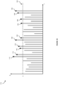
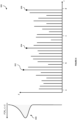
- Figures 1A and 1B illustrate two approaches for estimating extreme values within time series data.
- Figure 1A shows a first time-series plot 100 comprising a first plurality of time-based observations.
- the first time-series plot 100 shows a first plurality of extreme values 102, 104, 106 and a block 108.
- the first plurality of extreme values 102, 104, 106 correspond to a subset of the plurality of time-based observations determined according to the block maxima approach.
- the block maxima approach divides the data into several, sufficiently large, blocks and selects the maximum value within each block.
- the block 108 is shown between time points "a" and "b".
- the extreme value for the block 108 i.e. block a-b
- the values 104 and 106 represent the extreme values for blocks b-c and c-d respectively.
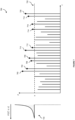
- Figure 1B shows a second time-series plot 110 comprising a second plurality of time-based observations.
- the second time-series plot 110 shows a second plurality of extreme values 112-130 determined according to the peaks-over-threshold (POT) approach based on a threshold 132.
- POT peaks-over-threshold
- the POT approach specifies a preferably large threshold such that only those values which exceed the threshold are considered extreme values for analysis and modelling.
- the values 112-130 are identified as exceeding the threshold 132 (i.e., the values are deemed to be threshold exceedances).
- the POT approach shown in Figure 1B captures a larger number of extreme values than the block maxima approach shown in Figure 1A .
- the extreme values can be used for further modelling and analysis. Typically, this involves fitting a statistical model of extremes to estimate the distribution of extreme values. This distribution is then used to forecast future extreme values.
- EVT can be applied to solve technical problems across a range of different technological applications. For example, within the domain of environmental monitoring, EVT can be used to predict the future concentration of pollutants in the atmosphere. Within the healthcare domain, EVT can be used to predict important biophysical quantities such as glucose level, heartbeat, and the like.
- a computer-implemented method for producing probabilistic forecasts of extreme values comprises obtaining input data comprising a plurality of signals of interest and a plurality of covariates associated therewith, each covariate of the plurality of covariates having an associated data type; performing a first forecast based on the input data, wherein performing the first forecast comprises: obtaining one or more trained machine learning models, each trained machine learning model of the one or more trained machine learning models having been trained to map one or more covariates of a respective data type to one or more surrogate covariates; mapping, using the one or more trained machine learning models and the input data, the plurality of covariates to one or more surrogate covariates, the one or more surrogate covariates corresponding to a compressed representation of the input data; fitting a statistical model of extremes to the plurality of signals of interest and the one or more surrogate covariates thereby generating a fitted statistical model of extremes, the statistical model of extremes being defined according to
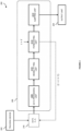
- Figure 2 shows a system 200 for forecasting extreme values according to an aspect of the present disclosure.
- the system 200 comprises a tracking device 202, an output unit 204, and a control device 206.
- the control device 206 comprises a data processing unit 208, a model fitting unit 210, a forecasting unit 212, and an alerting unit 214.
- the data processing unit 208 and the model fitting unit 210 form a part of the forecasting unit 212.
- the control device 206 is communicatively coupled to the tracking device 202 and the output unit 204.
- Figure 2 further shows data 216 received from the tracking device 202 at time step t and communicated to the control device 206.
- the system 200 is operable, at time step t, to receive data 216 from the tracking device 202 and determine a probabilistic forecast of extreme values at a future time step t + l . Based on this probabilistic forecast, an alert may be issued to the output unit 204 by the alerting unit 214.
- the data processing unit 208 receives data 216 from the tracking device 202 and performs further processing of this input data.
- One or more machine learning models are used to transform covariates of the input data to a compressed representation thereof.
- the compressed representation may have reduced dimensionality and/or be encoded to a smaller representation (i.e., fewer bits).
- the model fitting unit 210 fits a statistical model of extremes to the input data and the compressed representation.
- the forecasting unit 212 produces a probabilistic forecast of future extreme values based on the fitted statistical model of extremes.
- the alerting unit 214 analyses the probabilistic forecast of future extreme values produced by the forecasting unit 212 and, in accordance with a determination that the probabilistic forecast of future extreme values is indicative of a predicted extremal state occurring at one or more future time steps, causes an alert to be issued, via the output unit 204, to notify a user of the predicted extremal state.
- the system 200 provides an efficient process for producing probabilistic forecasts of extreme values.
- the system 200 may be employed within settings which require online forecasting of extreme values-i.e., applications whereby data is continuously received and used to update the model for forecasting extreme values.
- the system 200 allows forecasting of extreme values to be made for both univariate or multivariate and stationary or non-stationary data, thus enabling the systems and methods to be employed within a wide range of problem domains.
- multivariate modelling of extremes allows clusters of extreme events to be modelled.
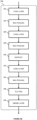
- Figure 3 shows a method 300, performed by components of the system 200 of Figure 2 , for producing probabilistic forecasts of extreme values according to an aspect of the present disclosure.
- the method 300 comprises the steps of obtaining 302 input data comprising a plurality of signals of interest and a plurality of covariates associated therewith.
- the method 300 further comprises performing 304 a first forecast by obtaining 306 one or more machine learning models, mapping 308 the plurality of covariates to one or more surrogate covariates using the one or more machine learning models, fitting 310 a statistical model of extremes to the plurality of signals of interest and the one or more surrogate covariates, and obtaining 312 a probabilistic forecast of future extreme values based on the fitted statistical model of extremes.
- the method 300 further comprises causing 314 control of a controllable system based on the probabilistic forecast of future extreme values.
- the method 300 is performed by the control device 206 of Figure 2 .
- the data processing unit 208 is configured to perform the steps of obtaining 302, performing 304, and mapping 308.
- the model fitting unit 210 is configured to perform the step of fitting 310
- the forecasting unit 212 is configured to perform the step of obtaining 312.
- the alerting unit 214 is configured to perform the step of causing 314.
- Step 302 Obtaining Input Data
- the method 300 comprises the step of obtaining 302 input data.
- the input data comprises a plurality of signals of interest and a plurality of covariates associated therewith. Each covariate of the plurality of covariates has an associated data type.
- the signals of interest correspond to the observations to be modelled and forecast.
- the plurality of signals of interest may correspond to glucose levels, heart rate, concentration of atmospheric pollutants, voltage level, plant control parameters, and the like.
- the signals of interest may alternatively be referred to as signals, observations, or values.
- the signals of interest are either univariate or multivariate.
- a univariate signal of interest comprises only a single variable (i.e., a single dimension), whilst a multivariate signal of interest comprises multiple variables (i.e., a plurality of dimensions).
- the signals of interest are either stationary or non-stationary. In the stationary case, the statistical properties of the signal do not vary over time; for the non-stationary case, the statistical properties of the signal may vary over time.
- the covariates are typically time-dependent such that they are associated with the signals of interest at every time step. That is, each covariate temporally corresponds to one or more signal of interest. Unlike the signals of interest, the covariates may be obtained from numerous different sources and thus correspond to a range of different data types. For example, within an environmental monitoring setting, the covariates may include, for a given time point or period, meteorological data, traffic data, satellite imagery data, and the like, associated with the signals of interest. Each of these different data have a different data type such as float, integer, factor, image data types (e.g., a matrix or tensor of integer or float values), and the like. Therefore, each covariate is associated with a different data type such that the plurality of covariates comprises multiple data types.
- the input data may be obtained in several different ways.
- the input data is obtained by reading the plurality of signals of interest and the plurality of covariates from one or more files stored on a computer-readable medium.
- the plurality of signals of interest and different portions of the plurality of covariates may be stored in different files.
- the plurality of signals of interest may be stored in a first file
- covariates related to one data type may be stored in a second file
- covariates related to another data type may be stored in a third file.
- the input data is obtained by reading a portion of a data stream or reading only portion(s) of file(s) relating to the different data.
- Step 304 Performing a first forecast
- the method 300 further comprises the step of performing 304 a first forecast based on the input data.
- a first forecast involves producing a probabilistic forecast of extremes at one or more future time steps based on a statistical model fitted to the input data.
- the statistical model is defined by a distribution, the parameters of which are automatically estimated from the input data.
- one or more machine learning models are used to generate a compressed representation of the covariates, referred to as the surrogate covariates.
- the data can be provided in an online manner over a number of different iterations.
- the method 300 may be used in a wide variety of application areas such as those which use high-dimensional, high-complexity, input data over relatively short intervals (e.g., real time or near real time applications), and those which operate in a reduced computation environment (e.g., edge computing).
- the forecasting process may be repeated across multiple time steps.
- the statistical model is updated based on newly obtained input data.
- the model is updated without requiring the model to be fitted from scratch. This improves the efficiency of the forecasting process.
- the method 300 further comprises the step of obtaining further input data and performing a second forecast based on the further input data. Therefore, references below to operations performed as part of the first forecast are equally applicable to operations performed as part of a second forecast. Indeed, the forecasting may be repeated any number of times using further input data with the steps and operations described in relation to the first forecast being equally applicable thereto.
- Step 306 Obtaining one or more trained machine learning models
- the covariates are processed using one or more machine learning models to provide a compressed representation of the covariates, referred to as surrogate covariates. Therefore, the method 300 further comprises, as part of the first forecast, obtaining 306 one or more trained machine learning models. Each trained machine learning model of the one or more trained machine learning models having been trained to map one or more covariates of a respective data type to one or more surrogate covariates.
- the trained machine learning models not only provide a compressed representation of the covariates, but also allow multiple different data types to be combined into a single set of surrogate covariates.
- the plurality of input covariates may comprise covariates obtained from different sources having different data types.
- the covariates could include text data, image data, time-series data, and the like, all associated with the signals of interest.
- the wide range of different data types not only leads to a high-dimensional input space, but also presents difficulties when seeking to combine these data into a usable form.
- covariates from different sources can be combined into a single usable compressed representation.
- the one or more trained machine learning models comprise any suitable machine learning model. Although referred to as trained machine learning models, the underlying algorithms or models of the trained machine learning models may be supervised or unsupervised. Thus, the trained machine learning models may alternatively be referred to simply as machine learning models. In one embodiment, the one or more machine learning models comprise one or more unsupervised models. Examples of such models include, but are not limited to, empirical mode decomposition (EMD), principal components analysis (PCA), singular value decomposition (SVD), manifold learning (e.g., Isomap, locally linear embedding, etc.), and the like. Each model may be assigned to process a different data type. For example, an EMD model may be used to process time-series data whilst PCA may be used to handle image-based data.
- EMD empirical mode decomposition
- PCA principal components analysis
- SVD singular value decomposition
- manifold learning e.g., Isomap, locally linear embedding, etc.
- the one or more machine learning models comprise one or more supervised models. Examples of such models include, but are not limited to, support vector machines (SVMs), decision trees and random forests, regression models (e.g., Bayesian regression, linear regression, etc.), and the like.
- the one or more machine learning models include one or more trained neural networks. For example, a first trained neural network is used for time-series data whilst a second neural network is used for image-based data. An example neural network for time-series data is shown in Figure 4 .
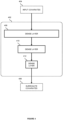
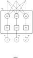
- Figure 4 shows a neural network architecture for mapping a plurality of covariates of the same data type to one or more surrogate covariates according to an embodiment of the present disclosure.
- FIG 4 shows a neural network 402 which receives input covariates 404 as input and outputs surrogate covariates 406.
- the neural network 402 comprises a first dense layer 408, a second dense layer 410, and a third dense layer 412.
- the input covariates 404 correspond to a vector of real values or integer values.
- the first dense layer 408 is a densely connected layer having, for example, 128 units. Each dimension of the input covariates 404 is connected to each unit of the first dense layer 408.
- the first dense layer 408 utilises a swish activation function. Alternatively, other activation functions are used such as ReLU, hyperbolic tangent (tanh), or sigmoid.
- the second dense layer 410 is a densely connected layer having, for example, 64 units.
- the second dense layer 410 comprises fewer units than the first dense layer 408 and more preferably comprises half as many units (or fewer) than the first dense layer 408.
- the second dense layer 410 utilises a swish activation function.
- activation functions are used such as ReLU, tanh, or sigmoid.
- the third dense layer 412 is a densely connected layer having a number of units equal to the target dimensionality of the surrogate covariates 406.
- the number of units in the third dense layer 412 is less than 64 and more preferably is less than 32. Yet more preferably, the number of units in the third dense layer 412 is less than 16 and more preferably again, the number of units in the third dense layer 412 is less than 10. Most preferably the number of units in the third dense layer 412 is equal to either one or three.
- the third dense layer 412 has a linear activation function.
- one or more machine learning models are used to map covariates of different data types to a single combined surrogate covariate.
- multiple neural networks are combined into a single architecture.
- a first neural network for time-series data is combined with a second neural network for image-based data to form a single monolithic model.
- a first neural network for textual data is combined with a second neural network for vector-valued data.
- this combined architecture is trained using a single training process and provides an efficient mechanism for mapping covariates of different data types to a combined compressed representation. This is shown in the example machine learning model of Figures 5A and 5B .
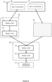
- Figure 5A shows a neural network architecture for mapping a plurality of covariates of two different data types to one or more surrogate covariates.
- the neural network architecture shown in Figure 5A is for mapping a vector-valued covariates and image-based covariates to one or more surrogate covariates.
- the neural network architecture in Figure 5A comprises a first neural network 502, a second neural network 504, and a third neural network 506. Whilst the three neural networks are illustrated as separate networks, they form a part of the same neural network architecture and are trained (and operate) as a single neural network.
- a plurality of covariates 507 comprises first input covariates 508 and second input covariates 510.
- the first input covariates 508 are vector-valued and the second input covariates 510 are image-based.
- the first neural network 502 receives first input covariates 508 as input
- the second neural network 504 receives second input covariates 510 as input
- the third neural network 506 receives as input the outputs of both the first neural network 502 and the second neural network 504.
- the third neural network 506 outputs one or more surrogate covariates 512.
- the first neural network 502 comprises a first dense layer 514 and a second dense layer 516.
- the architecture of the second neural network 504 is described in more detail in relation to Figure 5B below.
- the third neural network 506 comprises a first dense layer 518 and a second dense layer 520.
- the first neural network 502 receives vector-valued input covariates and is similar to the neural network 402 shown in Figure 4 .
- the first dense layer 514 corresponds to the first dense layer 408 of the neural network 402
- the second dense layer 516 corresponds to the second dense layer 410 of the neural network 402.
- the second neural network 504 receives image-based input covariates and is described in detail in relation to Figure 5B .
- Figure 5B shows the architecture of the second neural network 504 of Figure 5A .
- the second neural network 504 comprises a first convolutional layer 522, a first max pooling layer 524, a second convolutional layer 526, a second max pooling layer 528, a dropout layer 530, a third convolutional layer 532, a third max pooling layer 534, a flattening layer 536, and a dense layer 538.
- the second neural network 504 receives image-based data.
- the second neural network 504 receives three-channel image-based data such as RGB images or HSV images.
- Image-based data of width W and height H may be represented as a tensor of the form 1 ⁇ W ⁇ H ⁇ 3.
- the first convolutional layer 522 is a 3-dimensional convolutional layer having, for example, 64 output filters and a kernel size of (1, 3, 3) such that the 3D convolution window has a depth of 1, a height of 3, and a width of 3.
- the first convolutional layer 522 has a ReLU activation function. Alternatively, a swish, tanh, or sigmoid activation function may be used.
- the first max pooling layer 524 is a 3-dimensional max pooling layer having a pool size of (1, 2, 2) such that the second and third dimensions of the input to the first max pooling layer 524 are halved in size. Alternatively, other pool sizes may be used such that the second and third dimensions are reduced by a third, a quarter, a fifth, etc.
- the first max pooling layer 524 has a swish activation function. Alternatively, a ReLU, tanh, or sigmoid activation function may be used.
- the second convolutional layer 526 is a 3-dimensional convolutional layer having 32 output filters, a kernel size of (1, 3, 3), and a ReLU activation function.
- the second max pooling layer 528 is a 3-dimensional max pooling layer having a pool size of (1, 2, 2) and a swish activation function.
- the dropout layer 530 has a dropout rate of 0.25 such that 25% of the input units are dropped.
- the third convolutional layer 532 is a 3-dimensional convolutional layer having 16 output filters, a kernel size of (1, 3, 3), and a ReLU activation function.
- the third max pooling layer 534 is a 3-dimensional max pooling layer having a pool size of (1, 2, 2) and a swish activation function.
- the flattening layer 536 flattens the input to a 64-dimensional output shape.
- the dense layer 538 comprises 64 densely connected units and has a swish activation function.
- the dense layer 536 comprises any other number of densely connected units such as 32, 16, or 8 units.
- the dropout rate of the dropout layer 530 may be any other suitable value such as 0.75, 0.5, 0.3, 0.2, 0.1 or the like.
- the first dense layer 518 of the third neural network 506 is a densely connected layer having, for example, 128 units.
- the first dense layer 518 utilises a swish activation function.
- other activation functions are used such as ReLU, tanh, or sigmoid.
- the second dense layer 520 is a densely connected layer having a number of units equal to the target dimensionality of the one or more surrogate covariates 512.
- the number of units in the second dense layer 520 is less than 64 and more preferably is less than 32. Yet more preferably, the number of units in the second dense layer 520 is less than 16 and more preferably again, the number of units in the second dense layer 520 is less than 10. Most preferably the number of units in the second dense layer 520 is equal to one or three.
- the second dense layer 520 has a linear activation function.
- both the neural network architecture shown in Figure 4 and the neural network architecture shown in Figures 5A and 5B are trained using an Adam optimiser with a root mean squared error (RMSE) loss function.
- the weights within each neural network architecture are initialised using a Glorot Normal initialisation with all biases set to zero.
- a batch size of 64 with an epoch size of 1500 is used.
- the neural network architectures are trained such that the one or more surrogate covariates are closely correlated with the plurality of covariates.
- a training data set is used comprising a plurality of signals of interest, a plurality of covariates, and a corresponding plurality of parameters of the predetermined distribution of the statistical model of extremes.
- the neural network architectures are then trained using the above methodology on this training data such that the one or more surrogate covariates are closely correlated with the plurality of covariates (i.e., the RMSE between the plurality of parameters in the training data and the plurality of parameters produced using the surrogate covariates is minimised).
- Each machine learning model handles a different data type.
- the neural network architecture shown in Figures 5A and 5B map vector-valued and image-based covariates to surrogate covariates.
- a set of automated rules are employed. For example, a first rule routes the first input covariates 508 to the first neural network 502 and a second rule routes the second input covariates 510 to the second neural network 504.
- the rules examine the filename extension of the incoming covariates to determine which machine learning model can process the covariates.
- metadata accompanying the covariates is used to determine which machine learning model to use.
- Step 308 Mapping the plurality of covariates to one or more surrogate covariates
- the method 300 further comprises, as part of the first forecast, mapping 308, using the one or more trained machine learning models and the input data, the plurality of covariates to one or more surrogate covariates.
- the one or more surrogate covariates corresponding to a compressed representation of the input data.
- the one or more machine learning models are used to produce a compressed representation of the input data in the form of one or more surrogate covariates. This allows data from a variety of different sources to be used for model fitting (as described below).
- the modular approach of the present disclosure whereby each data type in the plurality of covariates is handled by a separate machine learning model, allows a rich variety of different data types to be used and aggregated to produce one or more covariates.
- the one or more machine learning models form a part of a single architecture (e.g., the neural network architecture shown in Figures 5A and 5B ) such that the one or more surrogate covariates are directly obtained from the output of the one or more machine learning models.
- the outputs of the one or more machine learning models are concatenated or otherwise combined to form the one or more surrogate covariates.
- Step 310 Fitting a statistical model of extremes
- the method 300 further comprises, as part of the first forecast, fitting 310 a statistical model of extremes to the plurality of signals of interest and the one or more surrogate covariates thereby generating a fitted statistical model of extremes.
- the statistical model of extremes being defined according to a predetermined distribution having a plurality of parameters.
- the step of fitting 310 may comprise obtaining a previously fitted statistical model of extremes and updating the plurality of parameters of the predetermined distribution according to the plurality of signals of interest and the one or more surrogate covariates.
- fitting a statistical model of extremes involves using either a block maxima approach or a peaks-over-threshold (POT) approach.
- POT peaks-over-threshold
- the choice of statistical model of extremes and predetermined distribution depends on factors such as the stationarity of the data and whether the data is univariate or multivariate.
- the statistical model of extremes is fitted using a block maxima approach as illustrated in Figure 6 .
- Figure 6 shows a plot 600 illustrating the block maxima approach to modelling extreme values.
- the plot 600 corresponds in part to the first time-series plot 100 shown in Figure 1 and comprises a plurality of extreme values 602, 604, 606 determined for blocks a-b, b-c, and c-d respectively.
- Figure 6 further shows a predetermined distribution 608.
- the block maxima approach divides the data into several, sufficiently large, blocks and selects the maximum value within each block.
- the distribution of the extreme values is then determined by fitting a suitable distribution, such as the generalised extreme value (GEV) distribution, to the extreme values.
- GEV generalised extreme value
- the blocks may be predetermined by the application domain or the standards of data recording. For example, yearly or quarterly maxima in environmental applications, and daily or hourly maxima in the health monitoring context. As such, in some implementations, the block size and the number of blocks are predetermined according to contextual information related to the problem domain.
- the step of fitting 310 a statistical model of extremes comprises first determining the extreme values for each block, and second fitting a GEV distribution to the observed extreme values (i.e., the extreme values determined in the first step).
- the predetermined distribution corresponds to the GEV distribution
- the values for the plurality of parameters of the predetermined distribution of Eq. 1 are determined using the maximum likelihood (ML) estimation method.
- the likelihood of the GEV model is built as the product of the GEV densities (obtained by taking the derivative of the distribution function of Eq. (1)) across the extremal data, L ⁇
- the ML estimation method comprises a numerical maximisation of the function L ( ⁇
- M ) is performed using an iterative method such as gradient descent, the Newton-Raphson method, or any quasi-Newton method.
- the plurality of parameters of the predetermined distribution of Eq. (1) are determined using a Markov chain Monte Carlo (MCMC) sampling technique.
- MCMC Markov chain Monte Carlo
- This method is based on pursuing the Bayesian approach to parameter estimation by treating parameters as random variables rather than unknown constants.
- q ( ⁇ ) which incorporates available information, or beliefs, about the parameter ⁇
- the aim of statistical estimation is to update the prior distribution density through the data and to obtain the posterior distribution density q ( ⁇
- the likelihood acts as an updating tool to improve knowledge about the parameter distribution.
- the prior q ( ⁇ ) is chosen as a multivariate normal distribution centred at a pilot estimate of the parameter ⁇ (e.g., based on past experience in the application domain) and standard deviation set initially as a large positive number (to emulate an almost flat "uninformative" prior) but afterwards tuned dynamically to ensure convergence to equilibrium.
- M ) is obtained as the equilibrium distribution density ⁇ ( ⁇ ) of a Markov chain ( ⁇ k ) where the next state ⁇ k +1 depends only on the present state ⁇ k .
- the Markov chain is implemented using a generalised acceptance-rejection sampling method. Namely, given the current state ⁇ of the chain, a new candidate state ⁇ ' is generated according to a proposal density ⁇ ( ⁇ '
- M min 1 q ⁇ ′
- the proposals are sampled from a normal distribution centred at the current state ⁇ of the Markov chain, with standard deviation set initially as a small positive number (to ensure a more careful exploration of the distribution landscape) but afterwards tuned dynamically to keep the acceptance rate within a predetermined range from 35% to 75%. Since such a proposal density is symmetric, ⁇ ( ⁇ '
- ⁇ ) ⁇ ( ⁇
- M min 1 L ⁇ ′
- the above acceptance-rejection sampling method is repeated until an equilibrium is reached.
- the equilibrium is monitored by standard diagnostic tools that may be implemented in an unsupervised manner. For example, the Gelman-Rubin diagnostic based on comparing parallel Markov chains.
- references are made in general to covariates, or more specifically to the one or more covariates.
- the skilled person will appreciate that these references may also refer to surrogate covariates, or the one or more surrogate covariates. That is, in embodiments where machine learning models are used to generate one or more surrogate covariates, the references below to covariates refer equally to surrogate covariates.
- the predetermined distribution of the block maximum M is a GEV-type approximation, P M ⁇ x
- C c ⁇ exp ⁇ 1 + ⁇ c x ⁇ ⁇ c ⁇ c + ⁇ 1 / ⁇ c x ⁇ R .
- the plurality of parameters of the predetermined distribution are then determined by estimating the latent functional dependency of the plurality of parameters upon the one or more covariates.
- the step of fitting 310 the statistical model of extremes may further comprise the step of determining the plurality of parameters by estimating the latent functional dependency of the plurality of parameters upon the one or more covariates.
- the latent functional dependency of the plurality of parameters upon the one or more covariates is estimated using one or more machine learning models.
- the one or more machine learning models correspond to a regression model comprising a plurality of regression parameters, wherein the one or more covariates correspond to explanatory variables of the regression model and the plurality of parameters correspond to dependent variables of the regression model.
- the values for the plurality of parameters of the predetermined distribution of Eq. (6) are determined using the maximum likelihood (ML) estimation method.
- the ML estimation method then proceeds with a numerical maximisation of the expression in Eq. (8), following a similar approach as described above in relation to Eq. (3), resulting in the ML estimates ( ⁇ j ) , ( k ⁇ j ), and ( m ⁇ j ).
- the values for the plurality of parameters of the predetermined distribution of Eq. (6) are determined using a Markov chain Monte Carlo (MCMC) sampling technique.
- MCMC Markov chain Monte Carlo
- the joint posterior density of the plurality of regression parameters is estimated using an MCMC estimator.
- the MCMC estimator obtains the joint posterior density of the plurality of regression parameters by combining a joint prior density of the plurality of regression parameters with the likelihood of the plurality of regression parameters based on the plurality of observed signals of interest and the one or more surrogate covariates.
- the acceptable-rejection sampling method as described above is used (i.e., with acceptance probability of the form in Eq. (5))
- the forecasting performed in the method 300 of Figure 3 at the step of performing 304 a forecast is repeated over several iterations such that, after a first forecast has been performed, further input data is obtained, and a second forecast is performed on the further input data.
- the joint posterior density of the plurality of parameters estimated during one iteration is used as the joint prior density of the plurality of parameters in a subsequent iteration. That is, when transitioning from a first forecast to a second forecast, the joint prior density of the plurality of parameters used during the second forecast corresponds to the joint posterior density of the plurality of parameters estimated during the first forecast.
- the distribution of the extreme value vectors is then determined by fitting a suitable distribution, such as the multivariate generalised extreme value (MGEV) distribution, to the observed multivariate block maxima.
- MGEV multivariate generalised extreme value
- Fitting the predetermined distribution of Eq. (10) comprises determining values for the plurality of parameters which best model the observed multivariate extreme values M 1 , ..., M n in n blocks. The fitted statistical model of extremes is thus generated by determining the plurality of parameters for the predetermined distribution.
- the values for the plurality of parameters of the predetermined distribution of Eq. (10) are determined using the maximum likelihood (ML) estimation method.
- the likelihood of the MGEV model is given as the product across the extremal data of the MGEV densities obtained as the p-th order partial derivative of the distribution function of Eq. (10), L ⁇
- ⁇ ⁇ p G x 1 , ... , x p ⁇ x 1 ... ⁇ x p .
- the ML estimation method comprises a numerical maximisation of the likelihood function L ( ⁇
- ( M i )) specified in Eq. (12) with respect to the vector parameter ⁇ ( ⁇ , ⁇ , ⁇ , w , ⁇ ).
- the respective maximiser ⁇ ( ⁇ , ⁇ , ⁇ , ⁇ , ⁇ ) is the resulting maximum likelihood estimate.
- ( M i )) is performed using an iterative method such as gradient descent, the Newton-Raphson method, or any quasi-Newton method.
- the plurality of parameters of the predetermined distribution of Eq. (30) are determined using a Markov chain Monte Carlo (MCMC) sampling technique.
- MCMC Markov chain Monte Carlo
- the joint posterior density of the plurality of parameters is estimated using an MCMC estimator.
- the MCMC estimator obtains the joint posterior density of the plurality of parameters by combining a joint prior density of the plurality of parameters with the likelihood of the plurality of parameters of Eq. (12) based on the plurality of observed block maxima M 1 , ..., M n .
- the acceptable-rejection sampling method as described above is used (i.e., with acceptance probability of the form in Eq. (5)).
- the statistical model of extremes is fitted using a peaks-over-threshold (POT) approach. This is illustrated in Figure 7 .
- POT peaks-over-threshold
- Figure 7 shows a plot 700 illustrating the peaks-over-threshold (POT) approach to modelling extreme values.
- the plot 700 shows a plurality of extreme values 702-720 determined as exceedances above a threshold 722, u . As such, the plot 700 corresponds in part to the second time-series plot 110 shown in Figure 1B and as explained above. Figure 7 further shows a predetermined distribution 724.
- the POT approach specifies a preferably large value for the threshold 722, u , such that only those signals of interest which exceed the threshold 722 are considered extreme values.
- the distribution of the extreme values is then determined by fitting a suitable distribution, such as the generalised Pareto distribution (GPD), to the extreme values. This is illustrated in Figure 7 by the predetermined distribution 724 which corresponds to a GPD distribution fitted to the plurality of extreme values 702-720.
- GPD generalised Pareto distribution
- the step of fitting 310 a statistical model of extremes comprises first determining the threshold, u , and second fitting a GPD distribution to the extreme values.
- the threshold, u is determined based on a balance between the accuracy of statistical approximation via the Pareto model (demanding higher thresholds) and the quality of statistical estimation of the model parameters from available exceedances (which would get depleted due to higher thresholds).
- the threshold is chosen according to an empirical quantile; for instance at a 95% level, so that about 5% of observed values lie above this threshold. This empirical approach is particularly useful for initial calibration of the model (e.g., at a piloting stage).
- thresholds of interest are determined by the subject matter. For example, an outside air concentration of nitrogen dioxide (NO 2 ) above 200 ⁇ g/m 3 (according to Euro 6 emission standards), or the glucose level above 140 mg/dL (for non-diabetic patients).
- shape ⁇ usually assumed not to depend on the threshold, u
- the ML estimation method proceeds with a numerical maximisation of the expression in Eq. (19) resulting in ML estimates ⁇ , ⁇ u , and ⁇ u .
- the plurality of parameters of the predetermined distribution of Eq. (15) are determined using a Markov chain Monte Carlo (MCMC) sampling technique.
- MCMC Markov chain Monte Carlo
- the joint posterior density of the plurality of parameters is estimated using an MCMC estimator.
- the MCMC estimator obtains the joint posterior density of the plurality of parameters by combining a joint prior density of the plurality of parameters with the likelihood of the plurality of parameters (Eq. (19)) based on the plurality of observed signals of interest and the one or more surrogate covariates.
- the acceptable-rejection sampling method as described above is used.
- the forecasting performed in the method 300 of Figure 3 at the step of performing 304 a forecast is repeated over several iterations such that, after a first forecast has been performed, further input data is obtained, and a second forecast is performed on the further input data.
- the joint posterior density of the plurality of parameters estimated during one iteration is used as the joint prior density of the plurality of parameters in a subsequent iteration. That is, when transitioning from a first forecast to a second forecast, the joint prior density of the plurality of parameters used during the second forecast corresponds to the joint posterior density of the plurality of parameters estimated during the first forecast.
- the plurality of parameters of the predetermined distribution are then determined by estimating the latent functional dependency of the plurality of parameters upon the one or more surrogate covariates.
- the step of fitting 310 the statistical model of extremes may further comprise the step of determining the plurality of parameters by estimating the latent functional dependency of the plurality of parameters upon the one or more surrogate covariates.
- the latent functional dependency of the plurality of parameters upon the one or more surrogate covariates is estimated using one or more machine learning models.
- the one or more machine learning models correspond to a regression model comprising a plurality of regression parameters, wherein the one or more surrogate covariates correspond to explanatory variables of the regression model and the plurality of parameters correspond to dependent variables of the regression model.
- the above parameterisation in Eq. (21) and Eq. (22) assumes that the threshold u remains stable. That is, it does not change between subsequent iterations of the forecasting process performed at the step of performing 304 a forecast. If the threshold were to be replaced by u + v (where v « u, i.e., the increment v is small as compared to the original threshold u), then the statistical model of extremes would need to be rebuilt and estimated from scratch to account for the new threshold.
- the lack of threshold stability for the parameterisation in Eq. (21) and Eq. (22) thus results in increased use of processing resources and time thereby limiting the applicability of the model for online processing.
- any suitable calibration threshold u 0 in Eq. (24) and Eq. (25) may be used provided it is close to the required range of thresholds u (so that the difference u - u 0 is small as compared to u).
- the calibration threshold u 0 is selected for the sake of computational convenience, for example, as a 95% empirical quantile of the pooled data.
- the threshold stability achieved by Eq. (24) and Eq. (25) also resolves the problem of entanglement of parameters. This problem occurs when a small change in one parameter leads to significant changes in other parameters. The resolution of this problem therefore allows a more efficient determination of the plurality of parameters to be made.
- the values for the plurality of parameters of the predetermined distribution of Eq. (20), given the linear-regression parameterisation of Eq. (26), are determined using the maximum likelihood (ML) estimation method.
- ML maximum likelihood
- the ML estimation method then proceeds with a numerical maximisation of the expression in Eq. (27), following a similar approach as described above in relation to Eq. (3), resulting in the ML estimates ( â j ),( b ⁇ j ), and ( ⁇ j ) .
- the values for the plurality of parameters of the predetermined distribution of Eq. (20) are determined using the Markov chain Monte Carlo (MCMC) sampling technique as described above.
- MCMC Markov chain Monte Carlo
- a joint posterior density of the plurality of regression parameters is estimated using an MCMC, estimator.
- the MCMC estimator obtains the joint posterior density of the plurality of regression parameters by combining a joint prior density of the plurality of regression parameters with the likelihood of the plurality of regression parameters based on the plurality of observed signals of interest and the one or more surrogate covariates.
- the regression-type specification of Eq. (24) is used to map the plurality of regression parameters to the plurality of parameters of the predetermined distribution.
- the forecasting performed in the method 300 of Figure 3 at the step of performing 304 a forecast is repeated over several iterations such that, after a first forecast has been performed, further input data is obtained, and a second forecast is performed on the further input data.
- the joint posterior density of the plurality of regression parameters estimated during one iteration is used as the joint prior density of the plurality of regression parameters in a subsequent iteration. That is, when transitioning from a first forecast to a second forecast, the joint prior density of the plurality of regression parameters used during the second forecast corresponds to the joint posterior density of the plurality of regression parameters estimated during the first forecast.
- the plot 700 illustrates the POT approach for the case whereby the plurality of signals of interest are univariate.
- This approach may be extended for multivariate signals of interest by replacing the predetermined distribution with a multivariate generalised Pareto distribution (MGPD).
- MGPD multivariate generalised Pareto distribution
- the first step in fitting the statistical model of extremes is to determine the threshold, u.
- G( x ) is a multivariate GEV distribution function
- G x G * 1 + ⁇ x ⁇ ⁇ ⁇ + 1 / ⁇
- G * x ⁇ exp ⁇ m * x , x ⁇ 0 0 otherwise
- MCMC Markov chain Monte Carlo
- the MCMC estimator obtains the joint posterior density of the plurality of parameters by combining a joint prior density of the plurality of parameters with the likelihood of the plurality of parameters based on the plurality of observed signals of interest and the one or more surrogate covariates.
- the forecasting performed in the method 300 of Figure 3 at the step of performing 304 a forecast is repeated over several iterations such that, after a first forecast has been performed, further input data is obtained, and a second forecast is performed on the further input data.
- the joint posterior density of the plurality of parameters estimated during one iteration is used as the joint prior density of the plurality of parameters in a subsequent iteration. That is, when transitioning from a first forecast to a second forecast, the joint prior density of the plurality of parameters used during the second forecast corresponds to the joint posterior density of the plurality of parameters estimated during the first forecast.
- the non-stationarity of the plurality of signals of interest, ( X (t)), is captured by treating the parameters of the predetermined distribution of Eq. (34) as functions of the one or more covariates, C (t)., leading to the predetermined distribution P X u t ⁇ x
- the plurality of parameters of the predetermined distribution of Eq. (37) are then determined by estimating the latent functional dependency of the plurality of parameters upon the one or more surrogate covariates.
- the step of fitting 310 the statistical model of extremes may further comprise the step of determining the plurality of parameters by estimating the latent functional dependency of the plurality of parameters upon the one or more surrogate covariates.
- the latent functional dependency of the plurality of parameters upon the one or more surrogate covariates is estimated using one or more machine learning models.
- the one or more machine learning models correspond to a regression model comprising a plurality of regression parameters, wherein the one or more surrogate covariates correspond to explanatory variables of the regression model and the plurality of parameters correspond to dependent variables of the regression model.
- the calibration threshold u 0 is selected for the sake of computational convenience, for example, as the vector of 95% empirical quantiles in each component of the pooled data.
- the vector coefficients ⁇ ( c ) and ⁇ ( c ) are functions of the one or more covariates c ⁇ R m subject to the constraint ⁇ ( c ) + ( u - u 0 ) ⁇ ( c ) > 0 , while ⁇ ( c ) must guarantee that the right-hand side of Eq. (39) stays negative.
- the predetermined distribution MGPD is fully specified and is thus usable for forecasting future extremes at the required time step(s).
- the plurality of parameters of the predetermined distribution of Eq. (37) are estimated using the Markov chain Monte Carlo (MCMC) sampling technique using the acceptance probability analogous to Eq. (5) as described above.
- MCMC Markov chain Monte Carlo
- a joint posterior density of the plurality of regression parameters is estimated using an MCMC, estimator.
- the MCMC estimator obtains the joint posterior density of the plurality of regression parameters by combining a joint prior density of the plurality of regression parameters with the likelihood of the plurality of regression parameters based on the plurality of observed signals of interest and the one or more surrogate covariates.
- the forecasting performed in the method 300 of Figure 3 at the step of performing 304 a forecast is repeated over several iterations such that, after a first forecast has been performed, further input data is obtained, and a second forecast is performed on the further input data.
- the joint posterior density of the plurality of regression parameters estimated during one iteration is used as the joint prior density of the plurality of regression parameters in a subsequent iteration. That is, when transitioning from a first forecast to a second forecast, the joint prior density of the plurality of regression parameters used during the second forecast corresponds to the joint posterior density of the plurality of regression parameters estimated during the first forecast.
- the forecasting performed in the method 300 of Figure 3 at the step of performing 304 obtains a fitted statistical model of extremes defined according to a predetermined distribution.
- Both the predetermined distribution and the means by which the plurality of parameters of the predetermined distribution are obtained are dependent on the approach taken (e.g., block maxima or POT), the stationarity of the data, and whether the data is univariate or multivariate.
- the fitted statistical model of extremes comprises a predetermined distribution comprising a plurality of parameters having values determined as a result of the fitting.
- the fitted statistical model of extremes is then employed to provide probabilistic forecasts of future extreme values.
- Step 312 Obtaining a probabilistic forecast of future extremes
- the method 300 further comprises, as part of the first forecast, obtaining 312 a probabilistic forecast of future extreme values based on the fitted statistical model of extremes for one or more future time steps.
- the fitted statistical model of extremes is used to produce probabilistic forecasts of future extreme values.
- the plurality of parameters of the predetermined distribution of the fitted statistical model of extremes are used to produce probabilistic forecasts of future extreme values.
- the probabilistic forecast of future extreme values includes a point estimate and, optionally, credible intervals obtained by the fitted statistical model of extremes for the one or more future time steps.
- the probabilistic forecast of future extreme values further comprises an exceedance probability.
- the probabilistic forecast of future extremes is obtained analytically using the explicit form of the fitted statistical model of extremes.
- the probabilistic forecast of future extremes is obtained empirically by simulating the fitted statistical model of extremes samples.
- the analytical properties of the MGPD which are required for the calculation of confidence regions, future return levels, and for efficient sampling from the MGPD, are difficult to obtain.
- samples are simulated from the MGPD.
- this provides an efficient method for sampling from the MGPD which is both direct (i.e., unsupervised) and universal (i.e., the range of simulated vector values covers the entire domain of the multivariate extremes).
- f z z ⁇ 1 p ⁇ 1 ⁇ p z ⁇ ⁇ 1 ⁇ z ⁇ ⁇ p z ⁇ z 0 + p ⁇ 1 z 0 ⁇ p ⁇ 1 ! , z > 0 .
- Step 314 Causing control of a controllable system
- the method 300 further comprises the step of causing 314 control of a controllable system based at least in part on the probabilistic forecast of future extremes.
- the probabilistic forecast of future extremes may be used to cause control of controllable systems such as blood glucose monitoring systems or environmental monitoring systems.
- the probabilistic forecast of future extremes is used to indicate whether a system is predicted to be in an extremal (e.g., abnormal) state at one or more future time points. If such an extremal state is forecasted to occur, the controllable system is controlled to account for this extremal state.
- control of the controllable system occurs through the issuance of a command or message to the controllable system indicating the probabilistic forecast of future extremes.
- the probabilistic forecast of future extremes is obtained as part of the operation of the controllable system such that the controllable system is able to account for the forecast directly.
- the exceedance probability may be used to determine whether control of the controllable system should occur. For example, if the exceedance probability for a given future time step is low, then the method will not cause control of the controllable system (even if the predicted point estimate or credible intervals indicate a high or low extreme value for the given future time step). Therefore, in some embodiments, the step of causing 314 is conditional on the exceedance probability being greater than a predetermined threshold.
- the predetermined threshold is preferably greater than 0.5 and less than or equal to 1.0. More preferably, the predetermined threshold probability is greater than 0.75 and more preferably again greater than 0.9. In one embodiment, the predetermined threshold probability is adjusted by a user thereby altering the sensitivity of the system to alerting a user of predicted future extreme value.
- the controllable system is controlled to attempt to avoid future extreme states occurring.
- predictively accounting for such extreme states may help improve the longevity and operation of the process.
- predictively accounting for such extreme states may help improve patient health by enabling preventative action to be taken before an extreme health state (e.g., high or low blood glucose, or high heart rate) occurs.
- an extreme health state e.g., high or low blood glucose, or high heart rate
- efficiently forecasting future extremes within such applications allows such preventative action to be taken quickly.
- a forecast is obtained by directly estimating the parameters of the statistical model of extremes using a trained deep learning model. This approach is shown in the method of Figure 8 .
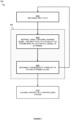
- Figure 8 shows a method 800 for producing probabilistic forecasts of extreme values according to an aspect of the present disclosure.
- the method 800 comprises the step of obtaining 802 input data and performing 804 a first forecast.
- the step of performing 804 the first forecast comprises the steps of mapping 806, using a machine learning model, the input data to a plurality of parameters of a statistical model of extremes, and obtaining 808 a probabilistic forecast of future extreme values.
- the method 800 further comprises the step of causing 810 control of a controllable system.
- the step of obtaining 802 input data in the method 800 corresponds to the step of obtaining 802 input data in the method 300 described in relation to Figure 3 above.
- the input data comprises a plurality of signals of interest and a plurality of covariates associated therewith.
- the method 800 further comprises the step of performing 804 a first forecast based on the input data.
- the first forecast corresponds to a probabilistic forecast of future extreme values obtained from the input data.
- the method 800 further comprises the step of obtaining further input data and performing a second forecast based on the further input data. Therefore, references below to operations performed as part of the first forecast are equally applicable to operations performed as part of a second forecast. Indeed, the forecasting may be repeated any number of times using further input data with the steps and operations described in relation to the first forecast being equally applicable thereto.
- the method 800 further comprises, as part of the first forecast, mapping 806, using a machine learning model, the input data to a plurality of parameters of a statistical model of extremes.
- the machine learning model corresponds to a trained machine learning model operable to map the plurality of signals and the plurality of covariates to a plurality of parameters of a predetermined distribution associated with the statistical model of extremes.
- the statistical model of extremes corresponds to a peaks-over-threshold (POT) approach with a generalised Pareto distribution (GPD) used as the predetermined distribution.
- POT peaks-over-threshold
- GPS generalised Pareto distribution
- a threshold, u is obtained e.g., from a user or empirically from the data.
- the neural network architectures described in relation to Figures 4 and 5A & B are used with a custom layer, described in relation to Figure 9 below, being appended to the end of each architecture.
- Figure 9 illustrates a custom neural network layer for estimating the plurality of parameters of a generalised Pareto distribution.
- Figure 9 shows a custom layer 902 for an artificial neural network such as the neural network 402 shown in Figure 4 and the third neural network 506 shown in Figure 5B .
- the custom layer comprises a first unit 904, a second unit 906, and a third unit 908.
- the first unit 904, the second unit 906, and the third unit 908 receive as input the three outputs of a previous layer (e.g., the outputs of the third dense layer 412 shown in Figure 4 or the outputs of the second dense layer 520 as shown in Figure 5B ).
- the output of the first unit 904 is fed to a first activation function 910
- the output of the second unit 906 is fed to a second activation function 912
- the output of the third unit 908 is fed to a third activation function 914.
- the custom layer 902 provides a first output 916, a second output 918, and a third output 920.
- the first output 916 i.e., the output of the first activation function 910) can be interpreted as an estimate of the shape parameter, ⁇ , of the GPD.
- the second output 918 can be interpreted as an estimate of the scale parameter, ⁇ , of the GPD.
- the third output 920 can be interpreted as an estimate of the exceedance probability, ⁇ .
- the custom layer 902 serves to estimate the latent functional dependency of the plurality of parameters upon the one or more surrogate covariates (e.g., as determined using the neural network architectures described in relation to Figure 4 and Figures 5A & 5B). Whilst the custom layer 902 is described primarily in reference to the neural network architectures described in relation to Figure 4 and Figures 5A & 5B , the skilled person will appreciate that the custom layer 902 may be appended to any suitable neural network architecture or machine learning model architecture.
- the neural network When mapping from a single covariate type (i.e., the neural network architecture of Figure 4 ) the three outputs of the third dense layer 412 of the neural network 402 are fed as input to the custom layer 902 Consequently, the neural network outputs a triplet of values corresponding to the shape ( ⁇ ) and scale ( ⁇ ) of the GPD along with the probability of threshold exceedance ( ⁇ ).
- the neural network architecture of Figures 5A and 5B When mapping from multiple covariate types (i.e., the neural network architecture of Figures 5A and 5B ) the three outputs of the second dense layer 520 of the third neural network 506 are fed as input to the custom layer 902. As before, the neural network thus outputs a triplet of values corresponding to the shape and scale of the GPD along with the exceedance probability.
- An artificial neural network incorporating the custom layer 902 is trained using an Adam optimiser with the following loss function, where ⁇ u ( c ) , ⁇ u ( c ) and ⁇ u ( c ) are the unknown functions of covariate vector c (given a fixed threshold u), which are estimated using a functional class implicitly determined by the neural network architecture, ( c i ) are the recorded values of covariates associated with the signals of interest ( X i ) , respectively, and L ( ⁇ u ( c i ), ⁇ u ( c i ), ⁇ u ( c i )
- X i ) is the likelihood per observation X i (cf. Eq.
- the penalty terms in Eq. (50) corresponds to restricting the gradient of the functions ⁇ u ( c ) , ⁇ u ( c ) and ⁇ u ( c ) with respect to variation of the vector argument c, with the tuning parameter ⁇ > 0.
- the value of ⁇ is set initially as any positive value, which is then adjusted as a hyper-parameter to optimise performance. Larger values of ⁇ lead to a slower varying output, while smaller values of ⁇ allow faster changes (i.e., bigger gradients).
- a batch size of 64 and an epoch size of 1500 are used and the weights are initialised using a Glorot Normal initialisation with all biases set to zero.
- the artificial neural network incorporating the custom layer 902 is trained on a training data set comprising a plurality of signals or interest and a plurality of covariates associated therewith along with a plurality of parameters of the predetermined distribution.
- the machine learning model thus estimates a plurality of parameters of the predetermined distribution directly from a plurality of covariates.
- the steps of obtaining 808 a probabilistic forecast of future extreme values and causing 810 control of a controllable system based on the probabilistic forecast correspond to the steps of obtaining 312 and causing 314 of the method 300 described in relation to Figure 3 above.
- the use of the above-described neural network architecture allows the parameters of the predetermined distribution to be directly estimated from the input data.
- a single machine learning model is trained to map the covariates of the input data into a compressed representation and subsequently obtain the plurality of parameters of the predetermined distribution. This provides a direct and efficient mechanism for forecasting future extreme values.
- the use of a single, monolithic, machine learning model to estimate the distribution parameters directly from the input data allows the forecasting method to be employed in application domains with limited computational resources.
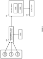
- Figure 10 shows a glucose monitoring system for producing probabilistic forecasts of extreme glucose levels.
- the glucose monitoring system comprises a tracking device 1002 comprising at least one sensor 1003 and an output unit 1004 configured to provide an output to a user.
- the output unit 1004 corresponds to a personal electronic device, such as a smartwatch or the like, and comprises a screen 1006 and a sensor 1008.
- the glucose monitoring system further comprises a control device 1010 communicatively coupled to the tracking device 1002 via a first communication channel 1012 and communicatively coupled to the output unit 1004 via a second communication channel 1014.
- the control device 1010 comprises a forecasting unit 1016 and an alerting unit 1018.
- the at least one sensor 1003 of the tracking device 1002 is configured to measure a blood glucose level of a user of the tracking device 1002.
- the control device 1010 receives blood glucose measurements from the tracking device 1002.
- the blood glucose measurements are received periodically (e.g., every 1 second, 5 seconds, 10 seconds, 30 seconds, 1 minute, 5 minutes, etc.) or, alternatively, are received upon sending a request from the control device 1010 to the tracking device 1002.
- the control device 1010 is further configured to receive a plurality of covariates corresponding to other biophysical signals received from a personal device of the user (e.g., as received by the sensor 1008 of the output unit 1004).
- the blood glucose measurements and the plurality of covariates are temporally aligned by timestamps included in the data.
- the forecasting unit 1016 is configured to perform the steps of method 300 as described in relation to Figure 3 above and/or the steps of the method 800 as described in relation to Figure 8 above. As such, the forecasting unit 1016 obtains input data comprising glucose measurements (i.e., the plurality of signals of interest) and a plurality of covariates associated therewith and produces a probabilistic forecast of future extreme values corresponding to future extreme glucose levels.
- glucose measurements i.e., the plurality of signals of interest
- covariates associated therewith
- the method 300 is used.
- the one or more machine learning models comprise an empirical mode decomposition (EMD).
- EMD empirical mode decomposition
- POT peaks-over-threshold
- GPD generalised Pareto distribution
- the GPD are fitted using a Markov Chain Monte Carlo (MCMC) approach.
- MCMC Markov Chain Monte Carlo
- Both the first statistical model of extremes and the second statistical model of extremes are initially fitted using an MCMC algorithm on historical blood glucose measurements and corresponding covariates. Consequently, at the first iteration, fitting the statistical model of extremes comprises updating the parameters of the predetermined distribution based on the posterior distribution of the initial fitted statistical model of extremes.
- the forecasting unit 1016 obtains the plurality of covariates (e.g., from the sensor 1008 of the output unit 1004) and determines a probabilistic forecast of future extreme values based on the first and second fitted statistical model of extremes.
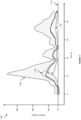
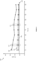
- Figure 11 shows a probabilistic forecast obtained from the fitted first statistical model of extremes.
- Figure 11 shows a plot 1100 of predicted glucose levels produced by the system of Figure 10 .
- the plot 1100 shows a probabilistic forecast of glucose levels comprising a mean 1102 shown as a dashed line, a 25% quantile 1104, and a 95% quantile 1106.
- the plot 1110 further shows the observed glucose levels 1108 shown as a solid line.
- the probabilistic forecast of glucose levels is obtained for a threshold 1110 set at 170 mg/dL.
- the mean 1102 of the fitted GPD closely tracks the observed glucose levels 1108.
- the alerting unit 1018 analyses the probabilistic forecast of future extreme values produced by the forecasting unit 1016.
- the probabilistic forecast of future extreme values comprises, for each time step, an exceedance probability, a point estimate (e.g., posterior mean or median), and a credible interval.
- the alerting unit 1018 compares the exceedance probability to a predetermined threshold probability corresponding to the minimum probability at which a user should be alerted of a predicted future extreme glucose level.
- the predetermined threshold probability is greater than 0.5 and less than or equal to 1.0. More preferably, the predetermined threshold probability is greater than 0.75 and more preferably again greater than 0.9.
- the predetermined threshold probability is adjusted by a user thereby altering the sensitivity of the system to alerting a user of predicted future extreme glucose levels.
- control device 1010 takes no further action and continues receiving input data and monitoring for future extremal states.
- the control device 1010 instructs the alerting unit 1018 to cause an alert to be issued via the output unit 1004.
- the alert is for notifying the user of the forecast extremal state (i.e., the forecast extremely high or low glucose level).
- the alert comprises a warning message displayed on the screen 1006 of the output unit 1004.
- the alert comprises a tactile or audible alert issued via the output unit 1004 such as a vibration or an audible alarm.
- the probabilistic forecast of future extreme values may thus be utilised to reduce the likelihood that a user experiences a hyperglycaemic or hypoglycaemic episode. By alerting the user of such an episode being predicted to occur the user can take early preventive action thereby reducing the likelihood of such an episode occurring.
- Figure 12 shows an environmental monitoring system for producing probabilistic forecasts of extreme air quality measures.
- the environmental monitoring system comprises a tracking device 1202, a control device 1204, and an output unit 1206.
- the tracking device 1202 corresponds to an environmental data collection system and comprises a nitrogen oxide sensor 1208, a nitrogen dioxide sensor 1210, and an ozone sensor 1212.
- the tracking device 1202 receives metadata 1214 in the form of one or more covariates corresponding to, for example, weather and traffic conditions temporally aligned to the observations received from the sensors.
- the control device 1204 comprises a forecasting unit 1216 and an alerting unit 1218.
- the output unit 1206 presents an output to one or more users of the system based on information received from the alerting unit 1218.
- the three sensors are placed at a fixed geographical location within a city centre to monitor the concentration of the three pollutants at that location over time.
- the one or more covariates, included as part of the metadata 1214 correspond to weather and traffic conditions and other environmental data (e.g., satellite imaging) associated with that geographical location.
- weather and traffic conditions and other environmental data e.g., satellite imaging
- timestamps are embedded within the observation data and the covariates.
- the forecasting unit 1216 is configured to perform the steps of method 300 as described in relation to Figure 3 above and/or the steps of the method 800 as described in relation to Figure 8 above. As such, the forecasting unit 1216 obtains input data comprising high-frequency (e.g., 15 minutes) maximum concentrations of nitrogen oxide (NO), nitrogen dioxide (NO 2 ), and ozone (O 3 ) from the nitrogen oxide sensor 1208, the nitrogen dioxide sensor 1210, and the ozone sensor 1212 respectively. The forecasting unit 1216 further obtains a plurality of covariates in the form of the metadata 1214 associated with the input data. The forecasting unit 1216 produces a probabilistic forecast of future extreme values corresponding to future extreme NO, NO 2 and/or O 3 levels. In one example implementation, the forecasting unit 1216 fits three statistical models of extremes, one for each pollutant. In an alternative implementation, the forecasting unit 1216 fits a single multivariate model of extremes for a combination of the three pollutants.
- NO nitrogen oxide
- NO 2 nitrogen dioxide
- O 3 o
- the forecasting unit 1216 periodically (e.g., every 15 minutes, every 30 minutes, etc.) receives input data and corresponding metadata, updates the statistical model(s) of extremes based on the received data, and produces a probabilistic forecast of future extreme concentrations of one or more of the three pollutants for one or more future time steps.
- the forecasting unit 1216 utilises an end-to-end machine learning model to estimate, for one of the pollutants, the plurality of parameters of a generalised Pareto distribution (GPD) from the input data and corresponding covariates.
- the plurality of covariates include tabular and image-based data.
- the tabular data comprises 81 covariates including timestamp information, traffic-related and meteorological variables (e.g., temperature, wind speed, wind direction, humidity, radiation, and traffic flow), lagged concentration values, and some time-dependent composite variables to account for the seasonal variability.
- the image-based data comprises 256x256 pixel RGB satellite images of the zones where the meteorological indicators were collected for the tabular data.
- a neural network architecture Prior to first use, a neural network architecture, such as that described in relation to Figures 5A and Figure 9 , is trained on a training dataset comprising 19,194 rows of tabular data and a corresponding set of 19,194 images. Further details regarding training such an architecture are given above in relation to Figure 8 .
- the forecasting unit 1216 utilises the trained neural network architecture to map from covariates to the parameters of the predetermined distribution. As the values of the covariates at a future time step (for which a prediction is sought) are not necessarily known, the probabilistic forecast of future extreme values is obtained for a future time step using the most recent covariates.
- the alerting unit 1218 analyses the probabilistic forecast of future extreme values produced by the forecasting unit 1216.
- the probabilistic forecast of future extreme values comprises a set of probabilities that a future extreme event will occur at one or more future time steps along with corresponding point estimates and credible intervals. For example, for a future time step corresponding to an hour in the future, the probabilistic forecast of future extreme values corresponds to the probability that an extreme event-in this case, an extremely high level an atmospheric pollutant such as NO, NO 2 , or O 3 -will occur along with a corresponding point estimate (e.g., posterior mean or median) and credible intervals. This is illustrated in Figure 13 .
- Figure 13 shows a plot 1300 of predicted extreme NO 2 levels produced by the system of Figure 12 .
- the plot 1300 shows a 25% quantile 1302, a 50% quantile 1304, and a 90% quantile 1306 of a fitted statistical model of extremes relating to NO 2 exceedances over time.
- the statistical model of extremes corresponds to a POT approach with a threshold 1308 set empirically at the 85% of the data.
- Figure 13 further shows a first region 1310 corresponding to the credible intervals for a first time point and a second region 1312 corresponding to the credible intervals for a second time point.
- the probability of a threshold exceedance at the first time point is estimated from the probabilistic forecast of future extreme values as 32% whilst the probability of a threshold exceedance at the second time point is estimated as 6%.
- the probability of a threshold exceedance at the second time point is much lower.
- Figure 13 Whilst the example shown in Figure 13 relates to univariate forecasting, the system described in Figure 12 may also be applied to multivariate forecasting. This is illustrated in Figure 14 .
- Figure 14 shows a quantile level plot 1400 of a probability distribution for a pair of pollutants produced by the system of Figure 12 .
- the quantile level plot 1400 shows a 50% quantile 1402, an 80% quantile 1404, a 90% quantile 1406, a 95% quantile 1408, a 99% quantile 1410, and an observation 1412.
- the quantiles (such as the 50% quantile 1402, etc.) are determined by the system of Figure 12 as a result of fitting an MGPD.
- the quantile level plot 1400 thus represents the multivariate probability distribution of a threshold exceedance for the pair of pollutants NO and NO 2 at a given time point.
- the alerting unit 1218 analyses the exceedance probability of the probabilistic forecast of future extreme values for a given future time step.
- the alerting unit 1218 compares the exceedance probability to a predetermined threshold probability corresponding to the minimum probability at which control of the controllable system should occur.
- the predetermined threshold probability is greater than 0.5 and less than or equal to 1.0. More preferably, the predetermined threshold probability is greater than 0.75 and more preferably again greater than 0.9.
- the predetermined threshold probability is adjusted by a user thereby altering the sensitivity of the system to causing control of the controllable system based on the predicted future extreme pollutant levels.
- causing control of the controllable system comprises issuing an alert to a user via the alerting unit 1218.
- the alert comprises a visible or audible warning displayed on a computer or device associated with the user.
- the alert comprises a command sent to an external system such as a traffic control system.
- the external system may then alter its operation based on the alert.
- a traffic control system upon receiving an alert indicating that an extreme level of atmospheric pollutants is predicted at a future time step for a geographical location, may alter traffic flow at that geographical location by rerouting traffic within the geographical location or preventing further traffic from entering the geographical location. The probabilistic forecast of future extreme values may thus be used to mitigate the likelihood of dangerous or harmful atmospheric pollutants building up within a geographical location.
- Figure 15 shows an example computing system for carrying out the methods of the present disclosure. Specifically, Figure 15 shows a block diagram of an embodiment of a computing system according to example aspects and embodiments of the present disclosure.
- Computing system 1500 can be configured to perform any of the operations disclosed herein such as, for example, any of the operations discussed with reference to Figures 2 to 8 .
- Computing system includes one or more computing device(s) 1502.
- One or more computing device(s) 1502 of computing system 1500 comprise one or more processors 1504 and memory 1506.
- One or more processors 1504 can be any general-purpose processor(s) configured to execute a set of instructions.
- one or more processors 1504 can be one or more general-purpose processors, one or more field programmable gate array (FPGA), and/or one or more application specific integrated circuits (ASIC).
- one or more processors 1504 include one processor.
- one or more processors 1504 include a plurality of processors that are operatively connected.
- processors 1504 are communicatively coupled to memory 1506 via address bus 1508, control bus 1510, and data bus 1512.
- Memory 1506 can be a random-access memory (RAM), a read-only memory (ROM), a persistent storage device such as a hard drive, an erasable programmable read-only memory (EPROM), and/or the like.
- One or more computing device(s) 1502 further comprise input/output (I/O) interface 1514 communicatively coupled to address bus 1508, control bus 1510, and data bus 1512.
- I/O input/output
- Memory 1506 can store information that can be accessed by one or more processors 1504.
- memory 1506 e.g. one or more non-transitory computer-readable storage mediums, memory devices
- the computer-readable instructions can be software written in any suitable programming language or can be implemented in hardware. Additionally, or alternatively, the computer-readable instructions can be executed in logically and/or virtually separate threads on one or more processors 1504.
- memory 1506 can store instructions (not shown) that when executed by one or more processors 1504 cause one or more processors 1504 to perform operations such as any of the operations and functions for which computing system 1500 is configured, as described herein.
- memory 1506 can store data (not shown) that can be obtained, received, accessed, written, manipulated, created, and/or stored.
- one or more computing device(s) 1502 can obtain from and/or store data in one or more memory device(s) that are remote from the computing system 1500.
- Computing system 1500 further comprises storage unit 1516, network interface 1518, input controller 1520, and output controller 1522.
- Storage unit 1516, network interface 1518, input controller 1520, and output controller 1522 are communicatively coupled via I/O interface 1514.
- Storage unit 1516 is a computer readable medium, optionally a non-transitory computer readable medium, comprising one or more programs, the one or more programs comprising instructions which when executed by one or more processors 1504 cause computing system 1500 to perform the method steps of the present disclosure.
- storage unit 1516 is a transitory computer readable medium.
- Storage unit 1516 can be a persistent storage device such as a hard drive, a cloud storage device, or any other appropriate storage device.
- Network interface 1518 can be a Wi-Fi module, a network interface card, a Bluetooth module, and/or any other suitable wired or wireless communication device.
- network interface 1518 is configured to connect to a network such as a local area network (LAN), or a wide area network (WAN), the Internet, or an intranet.
- LAN local area network
- WAN wide area network
- intranet an intranet
- Figure 15 illustrates one example computing system 1500 that can be used to implement the present disclosure.
- Other computing systems can be used as well.
- Computing tasks discussed herein as being performed at and/or by one or more functional unit(s) can instead be performed remote from the respective system, or vice versa.
- Such configurations can be implemented without deviating from the scope of the present disclosure.
- the use of computer-based systems allows for a great variety of possible configurations, combinations, and divisions of tasks and functionality between and among components.
- Computer-implemented operations can be performed on a single component or across multiple components.
- Computer-implemented tasks and/or operations can be performed sequentially or in parallel.
- Data and instructions can be stored in a single memory device or across multiple memory devices.
Landscapes
- Engineering & Computer Science (AREA)
- Physics & Mathematics (AREA)
- Theoretical Computer Science (AREA)
- General Physics & Mathematics (AREA)
- Data Mining & Analysis (AREA)
- Mathematical Physics (AREA)
- General Engineering & Computer Science (AREA)
- Software Systems (AREA)
- Life Sciences & Earth Sciences (AREA)
- Computing Systems (AREA)
- Artificial Intelligence (AREA)
- Evolutionary Computation (AREA)
- Computational Mathematics (AREA)
- Pure & Applied Mathematics (AREA)
- Computational Linguistics (AREA)
- Mathematical Optimization (AREA)
- Biophysics (AREA)
- Mathematical Analysis (AREA)
- General Health & Medical Sciences (AREA)
- Biomedical Technology (AREA)
- Health & Medical Sciences (AREA)
- Molecular Biology (AREA)
- Algebra (AREA)
- Probability & Statistics with Applications (AREA)
- Databases & Information Systems (AREA)
- Operations Research (AREA)
- Evolutionary Biology (AREA)
- Bioinformatics & Computational Biology (AREA)
- Bioinformatics & Cheminformatics (AREA)
- Management, Administration, Business Operations System, And Electronic Commerce (AREA)
Priority Applications (1)
| Application Number | Priority Date | Filing Date | Title |
|---|---|---|---|
| EP22179656.8A EP4293541A1 (de) | 2022-06-17 | 2022-06-17 | Systeme und verfahren zur probabilistischen vorhersage von extremen |
Applications Claiming Priority (1)
| Application Number | Priority Date | Filing Date | Title |
|---|---|---|---|
| EP22179656.8A EP4293541A1 (de) | 2022-06-17 | 2022-06-17 | Systeme und verfahren zur probabilistischen vorhersage von extremen |
Publications (1)
| Publication Number | Publication Date |
|---|---|
| EP4293541A1 true EP4293541A1 (de) | 2023-12-20 |
Family
ID=82839152
Family Applications (1)
| Application Number | Title | Priority Date | Filing Date |
|---|---|---|---|
| EP22179656.8A Pending EP4293541A1 (de) | 2022-06-17 | 2022-06-17 | Systeme und verfahren zur probabilistischen vorhersage von extremen |
Country Status (1)
| Country | Link |
|---|---|
| EP (1) | EP4293541A1 (de) |
Cited By (2)
| Publication number | Priority date | Publication date | Assignee | Title |
|---|---|---|---|---|
| CN117743280A (zh) * | 2024-02-21 | 2024-03-22 | 盈客通天下科技(大连)有限公司 | 一种公路桥梁施工数据智能管理方法 |
| CN119026120A (zh) * | 2024-10-28 | 2024-11-26 | 北京六方云信息技术有限公司 | 安全防护方法、装置、存储介质及计算机程序产品 |
Citations (3)
| Publication number | Priority date | Publication date | Assignee | Title |
|---|---|---|---|---|
| US20150235143A1 (en) * | 2003-12-30 | 2015-08-20 | Kantrack Llc | Transfer Learning For Predictive Model Development |
| GB2574233A (en) * | 2018-05-31 | 2019-12-04 | Ucl Business Plc | Apparatus and method for analysing MRI data |
| CN112734129A (zh) * | 2021-01-21 | 2021-04-30 | 中国科学院地理科学与资源研究所 | 基于非监督限制性优化的空气污染时空趋势预测方法 |
-
2022
- 2022-06-17 EP EP22179656.8A patent/EP4293541A1/de active Pending
Patent Citations (3)
| Publication number | Priority date | Publication date | Assignee | Title |
|---|---|---|---|---|
| US20150235143A1 (en) * | 2003-12-30 | 2015-08-20 | Kantrack Llc | Transfer Learning For Predictive Model Development |
| GB2574233A (en) * | 2018-05-31 | 2019-12-04 | Ucl Business Plc | Apparatus and method for analysing MRI data |
| CN112734129A (zh) * | 2021-01-21 | 2021-04-30 | 中国科学院地理科学与资源研究所 | 基于非监督限制性优化的空气污染时空趋势预测方法 |
Non-Patent Citations (4)
| Title |
|---|
| KIRKWOOD CHARLIE ET AL: "Bayesian Deep Learning for Spatial Interpolation in the Presence of Auxiliary Information", MATHEMATICAL GEOSCIENCES, SPRINGER BERLIN HEIDELBERG, BERLIN/HEIDELBERG, vol. 54, no. 3, 17 January 2022 (2022-01-17), pages 507 - 531, XP037812936, ISSN: 1874-8961, [retrieved on 20220117], DOI: 10.1007/S11004-021-09988-0 * |
| SILIUS M VANDESKOG ET AL: "Modelling sub-daily precipitation extremes with the blended generalised extreme value distribution", ARXIV.ORG, CORNELL UNIVERSITY LIBRARY, 201 OLIN LIBRARY CORNELL UNIVERSITY ITHACA, NY 14853, 21 May 2022 (2022-05-21), XP091213868 * |
| THIJSSEN BRAM ET AL: "Approximating multivariate posterior distribution functions from Monte Carlo samples for sequential Bayesian inference", PLOS ONE, vol. 15, no. 3, 13 March 2020 (2020-03-13), pages e0230101, XP093005500, Retrieved from the Internet <URL:https://journals.plos.org/plosone/article/file?id=10.1371/journal.pone.0230101&type=printable> [retrieved on 20221202], DOI: 10.1371/journal.pone.0230101 * |
| WANG HUI ET AL: "A novel non-homogeneous hidden Markov model for simulating and predicting monthly rainfall", THEORETICAL AND APPLIED CLIMATOLOGY, vol. 143, no. 1-2, 28 October 2020 (2020-10-28), pages 627 - 638, XP037326356, ISSN: 0177-798X, [retrieved on 20221209], DOI: 10.1007/S00704-020-03447-2 * |
Cited By (3)
| Publication number | Priority date | Publication date | Assignee | Title |
|---|---|---|---|---|
| CN117743280A (zh) * | 2024-02-21 | 2024-03-22 | 盈客通天下科技(大连)有限公司 | 一种公路桥梁施工数据智能管理方法 |
| CN117743280B (zh) * | 2024-02-21 | 2024-04-23 | 盈客通天下科技(大连)有限公司 | 一种公路桥梁施工数据智能管理方法 |
| CN119026120A (zh) * | 2024-10-28 | 2024-11-26 | 北京六方云信息技术有限公司 | 安全防护方法、装置、存储介质及计算机程序产品 |
Similar Documents
| Publication | Publication Date | Title |
|---|---|---|
| US12412111B2 (en) | Systems and methods for probabilistic forecasting of extremes | |
| EP3620983B1 (de) | Computerimplementiertes verfahren, computerprogrammprodukt und system zur datenanalyse | |
| Wang et al. | A hybrid approach for El Niño prediction based on Empirical Mode Decomposition and convolutional LSTM Encoder-Decoder | |
| Vandal et al. | Quantifying uncertainty in discrete-continuous and skewed data with Bayesian deep learning | |
| CN120197403B (zh) | 基于数字孪生的污水处理动态过程仿真预测方法及系统 | |
| EP2327019B1 (de) | Systeme und verfahren zur echtzeitklassifizierung und leistungsüberwachung von batch-prozessen | |
| US20210223765A1 (en) | Malfunction detection device, malfunction detection method, malfunction detection program, and recording medium | |
| EP3482354A1 (de) | Computersysteme und verfahren zur durchführung einer wurzelursachenanalyse und zum aufbau eines vorhersagemodells für seltene ereignisereignisse bei anlagenweiten operationen | |
| EP4293541A1 (de) | Systeme und verfahren zur probabilistischen vorhersage von extremen | |
| CN112163020A (zh) | 一种多维时间序列异常检测方法及检测系统 | |
| US20240012875A1 (en) | Method, system and computer readable medium for probabilistic spatiotemporal forecasting | |
| US20250133099A1 (en) | Sequential event modeling from multivariate categorical sensor data | |
| Koskela | Neural network methods in analysing and modelling time varying processes | |
| Zhou et al. | Combining recurrent neural networks with variational mode decomposition and multifractals to predict rainfall time series | |
| CN117196105A (zh) | 人数预测方法、装置、计算机设备、存储介质 | |
| Omar et al. | Single block encoder-decoder transformer model for multi-Step traffic flow forecasting | |
| CN120951739A (zh) | 一种基于孪生仿真的输电线路导线寿命预测方法及系统 | |
| CN116701875B (zh) | 一种特高压交流输电线路可听噪声概率预测方法及系统 | |
| Zhang et al. | IEnSF: Iterative Ensemble Score Filter for Reducing Error in Posterior Score Estimation in Nonlinear Data Assimilation | |
| Kumar et al. | Gru-lstm with attention-based forecasting for enhanced air quality | |
| Merkatas et al. | System identification using Bayesian neural networks with nonparametric noise models | |
| Gedda et al. | Change Point Detection for Process Data Analytics Applied to a Multiphase Flow Facility. | |
| Ma et al. | A recurrent gated unit-based mixture kriging machine Bayesian filtering approach for long-term prediction of dynamic intermittency | |
| ABDOU | A Comparative Study of Parameter Estimation Techniques in Linear Regression—Classical Approaches and Their Practical Implications | |
| EP4246376A1 (de) | Verfahren und systeme zur zeitreihenvorhersage unter fehlenden daten unter verwendung einer gemeinsamen imputierten und lerntechnik |
Legal Events
| Date | Code | Title | Description |
|---|---|---|---|
| PUAI | Public reference made under article 153(3) epc to a published international application that has entered the european phase |
Free format text: ORIGINAL CODE: 0009012 |
|
| STAA | Information on the status of an ep patent application or granted ep patent |
Free format text: STATUS: REQUEST FOR EXAMINATION WAS MADE |
|
| 17P | Request for examination filed |
Effective date: 20230815 |
|
| AK | Designated contracting states |
Kind code of ref document: A1 Designated state(s): AL AT BE BG CH CY CZ DE DK EE ES FI FR GB GR HR HU IE IS IT LI LT LU LV MC MK MT NL NO PL PT RO RS SE SI SK SM TR |
|
| STAA | Information on the status of an ep patent application or granted ep patent |
Free format text: STATUS: EXAMINATION IS IN PROGRESS |
|
| 17Q | First examination report despatched |
Effective date: 20240725 |