EP4336384A1 - Statistikrechner - Google Patents
Statistikrechner Download PDFInfo
- Publication number
- EP4336384A1 EP4336384A1 EP23195857.0A EP23195857A EP4336384A1 EP 4336384 A1 EP4336384 A1 EP 4336384A1 EP 23195857 A EP23195857 A EP 23195857A EP 4336384 A1 EP4336384 A1 EP 4336384A1
- Authority
- EP
- European Patent Office
- Prior art keywords
- value
- mean
- statistical measure
- dataset
- updated
- Prior art date
- Legal status (The legal status is an assumption and is not a legal conclusion. Google has not performed a legal analysis and makes no representation as to the accuracy of the status listed.)
- Pending
Links
Images







Classifications
-
- G—PHYSICS
- G06—COMPUTING OR CALCULATING; COUNTING
- G06F—ELECTRIC DIGITAL DATA PROCESSING
- G06F17/00—Digital computing or data processing equipment or methods, specially adapted for specific functions
- G06F17/10—Complex mathematical operations
- G06F17/18—Complex mathematical operations for evaluating statistical data, e.g. average values, frequency distributions, probability functions, regression analysis
Definitions
- the present disclosure concerns methods of determining statistical measures of a dataset. More particularly, but not exclusively, this disclosure concerns measures, including methods, apparatus and computer programs, for use in determining statistical measures of a dataset.
- Methods are known for estimating the mean, standard deviation and variance of a dataset, such as a set of signal samples in a communications system.
- Classical methods require the collection and storage of a large amount of data (large number of samples of the dataset) before any estimates of the mean, standard deviation and/or variance can be made. Furthermore, classical methods to calculate the variance require at least two passes over the whole dataset: one to calculate the mean of the dataset and a second to use this mean value when calculating the variance.
- Welford's method allows statistical measures such as the mean, variance and standard deviation to be calculated iteratively, as each sample of the dataset is received.
- this method suffers from a number of drawbacks. For example, it can suffer from data overflow issues when calculating the variance and standard deviation. This is because known implementations of Welford's method require storing a certain, ever-increasing, running sum.
- Welford's method is limited to real values and has not been adapted to complex values (e.g. in-phase ( I ) and quadrature ( Q ) components of a signal).
- a computer program comprising a set of instructions, which, when executed by computerised apparatus, cause the computerised apparatus to perform a method of determining a statistical measure of a dataset, the method comprising:
- apparatus for determining a statistical measure of a dataset comprising a processor configured to:
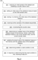
- Figure 1 is a flowchart corresponding to a method 100 of determining a statistical measure of a dataset according to embodiments of the disclosure.
- the method will generally be executed on a processor.
- the statistical measure can be one or more of: the mean, the variance and the standard deviation.
- the dataset could be, for example, a set of signal samples received in a communications system. Alternatively, the dataset could be a set of training inputs to a machine learning algorithm.
- the method begins at step 101 where an initial sample of the dataset is received by the processor and a counter value is initialised to zero. Then, at step 102, an initial value of the statistical measure (mean, variance and/or standard deviation) is set, based on the initial sample value. At step 103, the initial value of the statistical measure is stored in a memory. At step 104, further samples of the dataset are received by the processor sequentially, e.g. one by one. Each time a further sample is received, the method comprises applying steps 105 to 108 in sequence. At step 105, the counter value is incremented, i.e. increased by one.
- an updated value of the statistical measure is determined based on the previous, stored, value of the statistical measure, the current sample value (i.e. the new sample just received), and the current counter value (i.e. the incremented counter value).
- the stored value of the statistical measure in the memory is updated (i.e. overwritten) with the updated value of the statistical measure.
- it is determined whether or not a counter holding condition is met i.e. a condition according to which the counter value is frozen/held constant and is therefore no longer incremented as further new samples of the dataset are received.
- the method proceeds but without the step 105 of incrementing the counter value. In this manner, the counter value is held constant and further updated values of the statistical measure are determined by repeating steps 106 and 107 for each successive dataset sample received, where the "current counter value" is the "constant counter value”.
- This method 100 obtains values of the statistical measure iteratively, on a sample-by-sample basis and without needing to store a history of the whole dataset.
- the method 100 therefore uses much less memory than known techniques. There is also no requirement for costly memory access to large numbers of stored data (speeding up the process). No pre-analysis of the dataset is required, unlike the windowing method which requires an appropriate choice of window size to be determined. Furthermore, the method 100 does not employ a slow convolution process, unlike the windowing method.
- the method 100 accurately calculates the mean and variance (or standard deviation), which exactly agree with values obtained through classical methods during the early stages of the calculation (up until the counter holding condition is met).
- the method 100 is compatible with either real or complex dataset sample values.
- the counter holding condition is met when a counter upper limit is reached.
- the choice of counter upper limit may not necessarily be an arbitrary number, but may be based on considerations of counter overflow and/or counter underflow values. Overflow and underflow conditions arise when the precision limit supported by the processor is reached, such that numerical functions dependent on the counter value would no longer be accurate.
- the counter holding condition is met when a convergence condition is satisfied.
- the standard deviation, or the variance, of the dataset is monitored as each sample of the dataset is received.
- a difference function is evaluated, based on the difference between the standard deviation, or the variance, on a sample-by-sample basis. This difference function will tend to converge towards zero as the number of samples received increases. Accordingly, this allows a threshold difference function value to be set, below which it is determined that the convergence condition is satisfied and the counter can be frozen. Specific details of one such difference function, according to an embodiment, are provided below.
- Figure 2 is a flowchart corresponding to a further method 200 of determining a statistical measure of a dataset according to embodiments of the disclosure.
- the method will generally be executed on a processor.
- the statistical measure can be one or more of: the mean, the variance and the standard deviation.
- the dataset could be, for example, a set of signal samples received in a communications system. Alternatively, the dataset could be a set of training inputs to a machine learning algorithm.
- the method begins at step 201 where an initial sample of the dataset is received by the processor and a counter value is initialised to zero. Then, at step 202, an initial value of the statistical measure (mean, variance and/or standard deviation) is set, based on the initial sample value. At step 203, the initial value of the statistical measure is stored in a memory. At step 204, further samples of the dataset are received by the processor sequentially, e.g. one by one. Each time a further sample is received, the method comprises applying steps 205 to 208 in sequence. At step 205, the counter value is incremented, i.e. increased by one.
- an updated value of the statistical measure is determined based on the previous, stored, value of the statistical measure, the current sample value (i.e. the new sample just received), and the current counter value (i.e. the incremented counter value).
- the stored value of the statistical measure in the memory is updated (i.e. overwritten) with the updated value of the statistical measure.
- it is determined whether or not a counter reset condition is met i.e. a condition according to which the process should be reset back to an initial counter value of zero and the previous estimates of the statistical measure should be reset.
- the method in response to determining that the counter reset condition is met, the method reverts to the initial step 201, where the next received sample of the dataset is treated as the initial sample.
- This method 200 also, like the method 100 of Figure 1 , obtains values of the statistical measure iteratively, on a sample-by-sample basis and without needing to store a history of the whole dataset.
- the method 200 therefore uses much less memory than known techniques. There is also no requirement for costly memory access to large numbers of stored data (speeding up the process). No pre-analysis of the dataset is required, unlike the windowing method which requires an appropriate choice of window size to be determined. Furthermore, the method 200 does not employ a slow convolution process, unlike the windowing method.
- the method 200 accurately calculates the mean and variance (standard deviation), which exactly agree with values obtained through classical methods.
- the method 200 is compatible with either real or complex dataset sample values.
- This method 200 can detect/track sudden changes in the sample statistics, such as a step-like change in the sample mean, for example. This allows ongoing estimates of the mean and/or variance to recover rapidly from such a statistics change and continue to be accurate. This is in contrast to known windowing methods, which can require much more time to recover from sudden changes in the underlying sample statistics, depending on the window size chosen.
- an updated value of a gradient function is determined.
- the gradient function varies in response to changes in the statistics of the dataset, e.g. whether the mean of the samples is suddenly increasing or decreasing, or whether it is remaining approximately constant.
- the reset condition is considered to be met and the process is reset.
- the value of the gradient function is derived by comparing successive estimates of the mean of the dataset samples. In this manner, it is possible to detect a sudden upwards or downwards trend in the mean of the incoming samples, which is indicative of a sudden change in the underlying sample statistics. This can be carried out by determining an updated value of the mean of the dataset as each new sample is received. Then, by comparing the updated value of the mean to the previous value of the mean it is possible to determine an updated value of the gradient function based on the comparison between the updated value of the mean and the previous value of the mean.
- One option is to determine whether the updated value of the mean is greater than, the same as, or less than the previous value of the mean. Then, an output value can be provided which is indicative of whether the updated value of the mean is greater than, the same as, or less than the previous value of the mean.
- the output value is positive (e.g. +1) when the updated value of the mean is greater than the previous value of the mean; the output value is equal to 0 when the updated value of the mean is the same as the previous value of the mean; and the output value is negative (e.g. -1) when the updated value of the mean is less than the previous value of the mean.
- the value of the gradient function is derived by determining the mean of all calculated output values. In this manner, if the output values are predominately +1 for successive signal samples received after a certain point in time, the value of the gradient function will start to increase. If the output values are predominately -1 for successive signal samples received after a certain point in time, the value of the gradient function will start to decrease. It can be desirable to derive an always-positive value for the gradient function. This can be done by squaring the updated mean of the output values, for example.
- deriving the value of the gradient function can be done by comparing successive estimates of the mean of the dataset samples for the real and imaginary components of the samples separately. These outputs can then be combined to obtain a single, always-positive value of the gradient function.
- the methods disclosed herein can be used with datasets having real-valued samples and datasets having complex-valued samples and can be used to calculate either the mean and/or the variance (and by association the standard deviation) of the dataset on a sample-by-sample basis.
- ⁇ i is the updated value of the mean
- i is the current counter value
- x i is the current sample value
- the first mean estimate will be equal to the first sample, the next will be equal to the average of the first and second samples and so on, in an iterative manner, as further samples of the dataset are received.
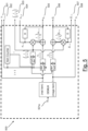
- Figure 3 shows an example hardware/firmware implementation 300 for iteratively calculating the mean of real-valued samples according to embodiments of the disclosure.
- the main input 301 receives the input samples x i .
- the output 302 provides the updated value of the mean ⁇ i .
- Three further outputs 303, 304, 305, are shown in Figure 3 . These are: the current counter value (i) 303; the next counter value (i + 1) 304, and the previous mean estimate ( ⁇ i -1 ) 305. These additional outputs are used if it is desired to calculate the variance or standard deviation, as is expanded upon below.
- Internally a number of processing blocks are employed to implement evaluation of the real-valued mean. These include division blocks 306, 307; a summation block 308; a multiplication block 309; the counter itself 310; and a delay block 311.
- Figure 4 shows an example hardware/firmware implementation 400 for iteratively calculating the variance of real-valued samples according to embodiments of the disclosure.
- the main input 401 receives the input samples x i .
- the implementation 300 of Figure 3 is used internally to calculate the mean.
- the outputs 402 and 403 are the current variance v i and the current mean ⁇ i respectively.
- the internal blocks used are defined with respect to the description of Figure 3 .
- Figure 5 shows an example hardware/firmware implementation 500 for iteratively calculating the mean of complex-valued samples according to embodiments of the disclosure.
- the main input 501a receives the current complex-valued input sample z i .
- a number of outputs 501-508 are provided. These are: the current sample real-component 501; the next counter value 502; the current counter value divided by the next counter value 503; the previous real-component of the mean 504; the current real-component of the mean 505; the current imaginary component of the mean 506; the previous imaginary component of the mean 507; and the current sample imaginary component 508.
- Outputs 505 and 506 correspond to the expressions above, the other (optional) outputs are utilised for calculating the variance of complex datasets, as explained below.
- the internal blocks used are defined with respect to the description of Figure 3 .
- Figure 6 shows an example hardware/firmware implementation 600 for iteratively calculating the variance of complex-valued samples according to embodiments of the disclosure.
- the main input 601 receives complex-valued input samples z i .
- the implementation 500 of Figure 5 is used internally to calculate the complex mean.
- the purposes of outputs 602 and 604 will become apparent from the discussion below.
- the internal blocks used are defined with respect to the description of Figure 3 .
- the counter holding condition is met when a convergence condition is satisfied.
- the standard deviation ⁇ i (which is the square root of the variance), or the variance v i , of the dataset is monitored as each sample of the dataset is received.
- a difference function is evaluated, based on the difference ⁇ i - ⁇ i -1 between the standard deviation (or the variance) on a sample-by-sample basis.
- An updated value of a difference function d p is determined based on the difference between the updated value of the standard deviation, or the variance, and the previous value of the standard deviation, or the variance.
- the positive envelope function is equal to the mean of the differences between the updated values of the standard deviation, or the variance, and the previous values of the standard deviation, when said differences are positive.
- the negative envelope function is equal to the mean of the differences between the updated values of the standard deviation, or the variance, and the previous values of the standard deviation, when said differences are negative.
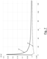
- Figure 7 shows an example plot of the positive and negative envelope functions as a function of the sample value i according to embodiments of the disclosure. Convergence of the two envelope curves is evident. A threshold value for the difference function could be said to be reached by a counter value of about 80-100, for example, at which point the counter value would be frozen/held constant.
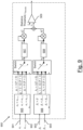
- Figure 8 shows an example hardware/firmware implementation 800 for calculating the real/complex mean and real/complex variance including the convergence evaluation using envelope functions as set out above according to embodiments of the disclosure.
- the implementation uses either the implementation 300 of Figure 3 or the implementation 500 of Figure 5 for calculating the means used to evaluate the positive and negative envelope functions.
- the implementation uses either the implementation 400 of Figure 4 or the implementation 600 of Figure 6 for evaluating the variance and mean.
- the input 801 receives the real or complex sample values.
- the outputs are: the standard deviation 802, the variance 803, and the real or complex mean 804.
- Comparator 805 is used to determine whether ⁇ i - ⁇ i- 1 , is less than zero or greater than/equal to zero.
- Comparator 806 is used to determine whether the value of the difference function d p is greater than or less than the threshold value d thresh .
- an updated value of a gradient function is determined.
- the gradient function varies in response to changes in the statistics of the dataset, e.g. whether the mean of the samples is suddenly increasing or decreasing, or whether it is remaining approximately constant.
- the reset condition is considered to be met and the process is reset.
- Figure 9 shows an example hardware/firmware implementation for determining values of a gradient function according to embodiments of the disclosure. This can be used to implement part of the method 200 of Figure 2 , where a reset condition is determined based on the value of the gradient function.
- inputs 901-904. These are: the current real component of the complex mean 901; the previous real component of the complex mean 902; the current imaginary component of the complex mean 903; and the previous imaginary component of the complex mean 904.
- a first comparator stage 905 compares the current real component of the complex mean with the previous real component of the complex mean.
- a second comparator stage 906 compares the current imaginary component of the complex mean with the previous imaginary component of the complex mean.
- the comparator stage 905, 906 outputs g i and h i are averaged on a sample-by-sample basis in statistics modules 907 and 908 respectively to obtain running means of the comparator outputs denoted G i and H i respectively.
- These statistics modules are, in an embodiment, the same as that of Figure 3 .
- a final comparator 909 determines if the value of the gradient function r i is greater than a threshold value r ithresh .
- Figure 10 shows an example hardware/firmware implementation 1000 which combines an implementation of the method 100 of Figure 1 with an implementation of the method 200 of Figure 2 according to embodiments of the disclosure.
- the main input 1001 receives samples of a dataset.
- a first block 600 is as per the implementation of Figure 6 , and calculates the complex mean and variance.
- Additional blocks 800 and 900 are based on the implementations of Figures 8 and 9 , and generate the counter freeze/stop signal and perform the gradient detection producing a reset signal.
- Three outputs 1002-1004 are provided. These are: the complex mean 1002, the standard deviation 1003 and the variance 1004.
- Figure 11 shows a comparison of estimating the mean of a dataset using a method according to the present disclosure and using a classical method.
- the classical method involves directly calculating the mean of the samples using a standard formula for the mean, and therefore requires storing all previous sample values.
- the plots are shown before the counter holding condition is met.
- Plot "A” is the real component of the mean obtained using a method according to the present disclosure
- plot "B” is the real component of the mean obtained using a classical method
- plot "C” is the imaginary component of the mean obtained using a method according to the present disclosure
- plot "D” is the imaginary component of the mean obtained using a classical method.
- the results obtained using a method according to the present disclosure are identical to the results obtained when using a classical method, when the counter holding condition has not yet been met.
- Figure 12 shows a comparison of estimating the variance of a dataset using a method according to the present disclosure and using a classical method.
- the classical method involves directly calculating the variance of the samples using a standard formula for the variance, and therefore requires storing all previous sample values and parsing of the data twice, as explained before.
- the plots are shown before the counter holding condition is met.
- Plot "A” is the variance obtained using a method according to the present disclosure; and plot "B” is the variance obtained using a classical method.
- the results obtained using a method according to the present disclosure are identical to the results obtained when using a classical method, when the counter holding condition has not yet been met.
- Figure 13 shows a comparison of estimating the mean (real component) of a dataset using a method according to the present disclosure (plot "C"), using a conventional windowing method (plot “B”), and using a classical method (plot “A”).
- the window size for the windowing method is set to 1024.
- the method according to the present disclosure and the classical method give identical results, whereas the conventional windowing shows a mean estimate that starts to ramp up to a comparable value as more of the window is occupied with estimates (this indicates a drawback of windowing during start up).
- the windowing method (plot “B”) takes 32 768 estimates before it is able to reflect values nearer to the classical mean estimation method
- the method according to the present disclosure (plot "C") is in immediate agreement with the classical method (plot "A”) and stays in agreement until the counter is frozen at the value of 32 768.
- both the windowing method and the method according to the present disclosure deviate from the classical mean estimate (as seen from the cut-out and expansions in Figure 15 and Figure 16 ).
- the method according to the present disclosure shows still closer agreement to the classical method (and therefore better performance) than the averaging window method does.
- Figures 17 to 19 show the ability of methods according to the present disclosure to cope with abrupt changes in dataset statistics.
- Figure 17 shows the real part of the complex mean for: a method according to the present disclosure (plot “C”); a windowing method (plot “B”); and a classical method (plot “A”).
- Figure 18 shows the imaginary part of the complex mean for: a method according to the present disclosure (plot "C”); a windowing method (plot "B”); and a classical method (plot "A”).
- Figure 19 shows the variance for: a method according to the present disclosure (plot “B”); and a classical method (plot “A”).
- the classical method exhibits overshoot and the windowing method takes several thousand counter intervals to recover from the abrupt change in sample statistics, whereas the method according to the present disclosure is able to quickly adapt to the change in statistics and continue produce a reliable estimate almost immediately after the change in statistics occurs.
- the dataset could comprise samples of a communications signal and the determined mean/variance could be used in an automatic gain control (AGC) system, for example.
- the dataset may comprise complex numbers corresponding to in-phase, I , and quadrature, Q , components of a signal.
- a further application may be found in machine learning.
- the dataset may comprise training inputs to a machine learning algorithm, and the determined mean/variance may be used to scale/normalise the training inputs.
- MMT Modern Portfolio Theory
- decisions can be generated as each data value is generated and dynamic trends observed
- Ongoing statistical surveys where all data cannot be collected in one instance, and/or where the survey covers a long time span, real-time statistical weather forecasting, health insurance, traffic flow on motorways and roads throughout the day and over periods of days, weeks, months, etc., continuous and ongoing manufacturing processes, etc.
- the methods as described above may each be comprised in or implemented in apparatus comprising a processor or processing system.
- the processing system may comprise one or more processors and/or memory.
- One or more aspects of the embodiments described herein comprise processes performed by apparatus.
- the apparatus comprises one or more processing systems or processors configured to carry out these processes.
- embodiments may be implemented at least in part by computer software stored in (non-transitory) memory and executable by the processor, or by hardware, or by a combination of tangibly stored software and hardware (and tangibly stored firmware).
- Embodiments also extend to computer programs, particularly computer programs on or in a carrier, adapted for putting the above described embodiments into practice.
- the program may be in the form of non-transitory source code, object code, or in any other non-transitory form suitable for use in the implementation of processes according to embodiments.
- the carrier may be any entity or device capable of carrying the program, such as a RAM, a ROM, or an optical memory device, etc.
Landscapes
- Engineering & Computer Science (AREA)
- Physics & Mathematics (AREA)
- Data Mining & Analysis (AREA)
- General Physics & Mathematics (AREA)
- Mathematical Optimization (AREA)
- Pure & Applied Mathematics (AREA)
- Theoretical Computer Science (AREA)
- Mathematical Physics (AREA)
- Computational Mathematics (AREA)
- Mathematical Analysis (AREA)
- Life Sciences & Earth Sciences (AREA)
- Operations Research (AREA)
- Probability & Statistics with Applications (AREA)
- Bioinformatics & Cheminformatics (AREA)
- Algebra (AREA)
- Evolutionary Biology (AREA)
- Databases & Information Systems (AREA)
- Software Systems (AREA)
- General Engineering & Computer Science (AREA)
- Bioinformatics & Computational Biology (AREA)
- Complex Calculations (AREA)
- Financial Or Insurance-Related Operations Such As Payment And Settlement (AREA)
Applications Claiming Priority (1)
| Application Number | Priority Date | Filing Date | Title |
|---|---|---|---|
| GB2213110.6A GB2622242A (en) | 2022-09-08 | 2022-09-08 | Statistics calculator |
Publications (1)
| Publication Number | Publication Date |
|---|---|
| EP4336384A1 true EP4336384A1 (de) | 2024-03-13 |
Family
ID=83945065
Family Applications (1)
| Application Number | Title | Priority Date | Filing Date |
|---|---|---|---|
| EP23195857.0A Pending EP4336384A1 (de) | 2022-09-08 | 2023-09-07 | Statistikrechner |
Country Status (2)
| Country | Link |
|---|---|
| EP (1) | EP4336384A1 (de) |
| GB (1) | GB2622242A (de) |
Cited By (1)
| Publication number | Priority date | Publication date | Assignee | Title |
|---|---|---|---|---|
| EP4645123A1 (de) * | 2024-04-29 | 2025-11-05 | Aptiv Technologies AG | Verfahren und system zur bestimmung eines mittelwertes und einer varianz von messdaten |
Citations (2)
| Publication number | Priority date | Publication date | Assignee | Title |
|---|---|---|---|---|
| US20090172064A1 (en) * | 2007-12-26 | 2009-07-02 | Juei-Chao Chen | Method for enhancing the computation of CSS and accuracy of computing hardware and to promote the computation speed |
| WO2019240638A1 (en) * | 2018-06-14 | 2019-12-19 | Telefonaktiebolaget Lm Ericsson (Publ) | Machine learning prediction of decoder performance |
-
2022
- 2022-09-08 GB GB2213110.6A patent/GB2622242A/en active Pending
-
2023
- 2023-09-07 EP EP23195857.0A patent/EP4336384A1/de active Pending
Patent Citations (2)
| Publication number | Priority date | Publication date | Assignee | Title |
|---|---|---|---|---|
| US20090172064A1 (en) * | 2007-12-26 | 2009-07-02 | Juei-Chao Chen | Method for enhancing the computation of CSS and accuracy of computing hardware and to promote the computation speed |
| WO2019240638A1 (en) * | 2018-06-14 | 2019-12-19 | Telefonaktiebolaget Lm Ericsson (Publ) | Machine learning prediction of decoder performance |
Non-Patent Citations (3)
| Title |
|---|
| ANDRE CARLON ET AL: "Multi-Iteration Stochastic Optimizers", ARXIV.ORG, CORNELL UNIVERSITY LIBRARY, 201 OLIN LIBRARY CORNELL UNIVERSITY ITHACA, NY 14853, 3 November 2020 (2020-11-03), XP081806189 * |
| GLAMOCANIN OGNJEN OGNJEN GLAMOCANIN@EPFL CH ET AL: "Built-in Self-Evaluation of First-Order Power Side-Channel Leakage for FPGAs", PROCEEDINGS OF THE 33RD ANNUAL ACM SYMPOSIUM ON USER INTERFACE SOFTWARE AND TECHNOLOGY, ACMPUB27, NEW YORK, NY, USA, 23 February 2020 (2020-02-23), pages 204 - 210, XP058727522, ISBN: 978-1-4503-7514-6, DOI: 10.1145/3373087.3375318 * |
| YASSIN YAHYA H YHYASSIN@GMAIL COM ET AL: "Algorithm/Architecture Co-optimisation Technique for Automatic Data Reduction of Wireless Read-Out in High-Density Electrode Arrays", ACM TRANSACTIONS ON EMBEDDED COMPUTING SYSTEMS, ACM, NEW YORK, NY, US, vol. 17, no. 3, 22 May 2018 (2018-05-22), pages 1 - 19, XP058676999, ISSN: 1539-9087, DOI: 10.1145/3190854 * |
Cited By (1)
| Publication number | Priority date | Publication date | Assignee | Title |
|---|---|---|---|---|
| EP4645123A1 (de) * | 2024-04-29 | 2025-11-05 | Aptiv Technologies AG | Verfahren und system zur bestimmung eines mittelwertes und einer varianz von messdaten |
Also Published As
| Publication number | Publication date |
|---|---|
| GB202213110D0 (en) | 2022-10-26 |
| GB2622242A (en) | 2024-03-13 |
Similar Documents
| Publication | Publication Date | Title |
|---|---|---|
| US8265742B2 (en) | Method, computer program, and system for automated real-time signal analysis for detection, quantification, and prediction of signal changes | |
| US20060190217A1 (en) | Particle sampling method and sensor fusion and filtering method | |
| WO2021184541A1 (zh) | 一种北斗变形监测中多路径误差的削弱方法 | |
| EP4336384A1 (de) | Statistikrechner | |
| CN115931055A (zh) | 一种基于大数据分析的农村供水运行诊断方法及系统 | |
| Dan et al. | An automatic real-time cable modal frequency identification and tracking algorithm by combining recursive band-pass filter and recursive Hilbert transform | |
| CN115932913B (zh) | 一种卫星定位伪距修正方法及装置 | |
| US7529651B2 (en) | Accurate linear parameter estimation with noisy inputs | |
| CN119756344A (zh) | 基于自适应mcmc的鲁棒因子图优化组合导航方法 | |
| CN119598399A (zh) | 一种面向智慧城市的物联网传感器数据融合方法 | |
| CN109344993A (zh) | 一种基于条件概率分布的河道洪峰水位预报方法 | |
| US20130034138A1 (en) | Time delay estimation | |
| CN109117965B (zh) | 基于卡尔曼滤波器的系统状态预测装置和方法 | |
| CN105429720A (zh) | 基于emd重构的相关时延估计方法 | |
| GB2622243A (en) | Statistics calculator | |
| Coburger et al. | Conditional point estimation in adaptive group sequential test designs | |
| RU2421754C2 (ru) | Способ определения поля скоростей воздушной массы посредством высокоразрешающего доплеровского анализа | |
| JP2005017266A (ja) | レーダ雨量測定装置及びその測定方法 | |
| CN117852156B (zh) | 一种基于贝叶斯的道路平面线位智能重构的方法及系统 | |
| CN114895298A (zh) | 一种雷达慢速弱机动目标量测修正伯努利滤波方法及装置 | |
| CN114740501A (zh) | 一种基于频域参数的卫星导航欺骗信号检测方法 | |
| CN115355910A (zh) | 一种基于二级Sigma点的UKF滤波算法 | |
| CN112699718B (zh) | 一种尺度和光照自适应的结构化多目标跟踪方法及其应用 | |
| Dembo et al. | On the parameters estimation of continuous-time ARMA processes from noisy observations | |
| Sopipan | Application of extreme value theory for maximum rainfall at nakhon ratchasima province |
Legal Events
| Date | Code | Title | Description |
|---|---|---|---|
| PUAI | Public reference made under article 153(3) epc to a published international application that has entered the european phase |
Free format text: ORIGINAL CODE: 0009012 |
|
| STAA | Information on the status of an ep patent application or granted ep patent |
Free format text: STATUS: THE APPLICATION HAS BEEN PUBLISHED |
|
| AK | Designated contracting states |
Kind code of ref document: A1 Designated state(s): AL AT BE BG CH CY CZ DE DK EE ES FI FR GB GR HR HU IE IS IT LI LT LU LV MC ME MK MT NL NO PL PT RO RS SE SI SK SM TR |
|
| STAA | Information on the status of an ep patent application or granted ep patent |
Free format text: STATUS: REQUEST FOR EXAMINATION WAS MADE |
|
| 17P | Request for examination filed |
Effective date: 20240911 |
|
| RBV | Designated contracting states (corrected) |
Designated state(s): AL AT BE BG CH CY CZ DE DK EE ES FI FR GB GR HR HU IE IS IT LI LT LU LV MC ME MK MT NL NO PL PT RO RS SE SI SK SM TR |