EP4425367A1 - Automatische bestimmung der lüftungsgitteröffnungsgrösse für die automation einer einrichtung zur numerischen simulation - Google Patents
Automatische bestimmung der lüftungsgitteröffnungsgrösse für die automation einer einrichtung zur numerischen simulation Download PDFInfo
- Publication number
- EP4425367A1 EP4425367A1 EP24160114.5A EP24160114A EP4425367A1 EP 4425367 A1 EP4425367 A1 EP 4425367A1 EP 24160114 A EP24160114 A EP 24160114A EP 4425367 A1 EP4425367 A1 EP 4425367A1
- Authority
- EP
- European Patent Office
- Prior art keywords
- grille
- computer
- geometry
- dimensional
- image
- Prior art date
- Legal status (The legal status is an assumption and is not a legal conclusion. Google has not performed a legal analysis and makes no representation as to the accuracy of the status listed.)
- Pending
Links
Images


Classifications
-
- G—PHYSICS
- G06—COMPUTING OR CALCULATING; COUNTING
- G06T—IMAGE DATA PROCESSING OR GENERATION, IN GENERAL
- G06T17/00—Three-dimensional [3D] modelling for computer graphics
- G06T17/20—Finite element generation, e.g. wire-frame surface description, tesselation
-
- G—PHYSICS
- G06—COMPUTING OR CALCULATING; COUNTING
- G06F—ELECTRIC DIGITAL DATA PROCESSING
- G06F30/00—Computer-aided design [CAD]
- G06F30/20—Design optimisation, verification or simulation
- G06F30/23—Design optimisation, verification or simulation using finite element methods [FEM] or finite difference methods [FDM]
-
- G—PHYSICS
- G06—COMPUTING OR CALCULATING; COUNTING
- G06F—ELECTRIC DIGITAL DATA PROCESSING
- G06F30/00—Computer-aided design [CAD]
- G06F30/20—Design optimisation, verification or simulation
-
- G—PHYSICS
- G06—COMPUTING OR CALCULATING; COUNTING
- G06F—ELECTRIC DIGITAL DATA PROCESSING
- G06F30/00—Computer-aided design [CAD]
- G06F30/10—Geometric CAD
- G06F30/17—Mechanical parametric or variational design
-
- G—PHYSICS
- G06—COMPUTING OR CALCULATING; COUNTING
- G06F—ELECTRIC DIGITAL DATA PROCESSING
- G06F30/00—Computer-aided design [CAD]
- G06F30/20—Design optimisation, verification or simulation
- G06F30/28—Design optimisation, verification or simulation using fluid dynamics, e.g. using Navier-Stokes equations or computational fluid dynamics [CFD]
-
- G—PHYSICS
- G06—COMPUTING OR CALCULATING; COUNTING
- G06T—IMAGE DATA PROCESSING OR GENERATION, IN GENERAL
- G06T15/00—Three-dimensional [3D] image rendering
- G06T15/005—General purpose rendering architectures
-
- G—PHYSICS
- G06—COMPUTING OR CALCULATING; COUNTING
- G06T—IMAGE DATA PROCESSING OR GENERATION, IN GENERAL
- G06T7/00—Image analysis
- G06T7/60—Analysis of geometric attributes
- G06T7/62—Analysis of geometric attributes of area, perimeter, diameter or volume
-
- G—PHYSICS
- G06—COMPUTING OR CALCULATING; COUNTING
- G06V—IMAGE OR VIDEO RECOGNITION OR UNDERSTANDING
- G06V10/00—Arrangements for image or video recognition or understanding
- G06V10/40—Extraction of image or video features
- G06V10/44—Local feature extraction by analysis of parts of the pattern, e.g. by detecting edges, contours, loops, corners, strokes or intersections; Connectivity analysis, e.g. of connected components
-
- G—PHYSICS
- G06—COMPUTING OR CALCULATING; COUNTING
- G06F—ELECTRIC DIGITAL DATA PROCESSING
- G06F2111/00—Details relating to CAD techniques
- G06F2111/10—Numerical modelling
-
- G—PHYSICS
- G06—COMPUTING OR CALCULATING; COUNTING
- G06F—ELECTRIC DIGITAL DATA PROCESSING
- G06F2113/00—Details relating to the application field
- G06F2113/08—Fluids
-
- G—PHYSICS
- G06—COMPUTING OR CALCULATING; COUNTING
- G06F—ELECTRIC DIGITAL DATA PROCESSING
- G06F2119/00—Details relating to the type or aim of the analysis or the optimisation
- G06F2119/14—Force analysis or force optimisation, e.g. static or dynamic forces
Definitions
- This disclosure relates to determining ventilation grille opening sizes and, more specifically, relates to automatic determination of ventilation grille opening sizes for numerical simulation setup automation in a computer-implemented environment.
- VR regions are also known as variable resolution (VR) regions and have sizes defined by separate referencing geometries. Specifically, for a Lattice-Boltzmann Method (LBM) based simulation, VR regions have varied lattice refinement sizes among different levels.
- LBM Lattice-Boltzmann Method
- a computer-implemented method includes automatically determining a ventilation grille opening size estimation for numerical simulation setup automation based on an input in a computer-implemented environment.
- the computer-implemented method includes creating screenshots of a plurality of computer-rendered images of a three-dimensional grille geometry, with the three-dimensional grille geometry disposed at a different angle of rotation about a first axis, identifying which, if any, of the screenshots has an image of the three-dimensional grille geometry with a total opening value that is larger than every other one of the screenshot three-dimensional grille geometry images, and designating the identified image as a target image for further processing to determine the ventilation grille opening size estimation.
- a computer-implemented method includes automatically determining a ventilation grille opening size estimation for numerical simulation setup automation based on an input in a computer-implemented environment.
- the computer-implemented method includes importing a three-dimensional grille geometry, calculating an oriented bounding box based on the three-dimensional grille geometry, identifying an initial viewing vector for the imported three-dimensional grille geometry, creating a spatial calibration box to associate a pixel domain of a computer-rendered image of the three-dimensional grille geometry and a physical domain for including a real-world version of a grille based on the three-dimensional grille geometry, screenshotting a series of computer-rendered images of the three-dimensional grille geometry from a perspective defined by the initial viewing vector and with the three-dimensional grille geometry disposed at different orientations (each orientation showing the image of the three-dimensional grille geometry at a different angle of rotation about a first axis), identifying which, if any, of the screenshot three-dimensional grille geometry images has
- a computer system is configured to automatically determine a ventilation grille opening size estimation for numerical simulation setup automation based on an input in a computer-implemented environment.
- the computer system includes a computer processor and computer-based memory operatively coupled to the computer processor, wherein the computer-based memory stores computer-readable instructions that, when executed by the computer processor, cause the computer-based system to: create screenshots of a plurality of computer-rendered images of a three-dimensional grille geometry, with the three-dimensional grille geometry disposed at a different angle of rotation about a first axis, identify which, if any, of the screenshots has an image of the three-dimensional grille geometry with a total opening value that is larger than every other one of the screenshot three-dimensional grille geometry images, and designate the identified image as a target image for further processing to determine the ventilation grille opening size estimation.
- a non-transitory computer readable medium has stored thereon computer-readable instructions that, when executed by a computer-based processor, cause the computer-based processor to automatically determine a ventilation grille opening size estimation for numerical simulation setup automation based on an input in a computer-implemented environment, by utilizing a process that includes creating screenshots of a plurality of computer-rendered images of a three-dimensional grille geometry, with the three-dimensional grille geometry disposed at a different angle of rotation about a first axis, identifying which, if any, of the screenshots has an image of the three-dimensional grille geometry with a total opening value that is larger than every other one of the screenshot three-dimensional grille geometry images, and designating the identified image as a target image for further processing to determine the ventilation grille opening size estimation.
- certain implementations facilitate the automatic creation of three-dimensional (3D) variable resolution regions for grille geometries that may be utilized in one or more computer-implemented simulations. More particularly, this is done in a manner that results in the simulations being conducted with great efficiency of computational resources - balancing the availability of such resources against the need for precision and detail in such simulations.
- Implementations of the systems and techniques disclosed herein help eliminate imprecision and errors in engineers' judgements, for example, when making measurements, estimations, setting VR regions, and/or attempting to simulate a grille or a particular environment that includes the grille. Improved accuracy and consistency may be realized.
- Implementations of the systems and techniques disclosed herein overcome technical challenges associated with identifying the location of openings and determining their sizes, especially in the presence of visual noise, such as horizontal/vertical bars and/or vehicle logos, and variations in shape of the grille openings/holes that vary across different vehicle models/designs.
- Implementations of the systems and techniques disclosed herein overcome technical challenges associated with spatial calibration being difficult due to a lack of good reference geometries, and the fact that in an automated simulation workflow, manual spatial calibration may not be feasible or practical.
- a "mesh” is network of cells and nodes that support certain numerical simulations in a computer-implemented environment. Typically, each cell in a mesh would represent an individual solution to the simulation and the various individual solutions may be combined to produce an overall solution for the entire mesh.
- Resolution refers to the density or size of cells (e.g., mesh size) or finite elements represented, for example, in a mesh generated by a computer to support a computer-implemented numerical simulation based on a computer-implemented model of an object or a portion thereof.
- Resolution can influence efficiency and effectiveness of a computer-implemented simulation. For example, high resolution simulations can produce detailed data but are costly, whereas low resolution simulations tend to be less expensive but produce less detailed data. Utilizing variable resolution ("VR”) regions is one way to try to strike a balance between the two.
- VR variable resolution
- a “variable resolution region” is a region (e.g., a flow region) defined in and/or around a modeled object (e.g., a grille) or portion of a modeled object in a computer-implemented simulation involving the modeled object (e.g., the grille or a vehicle or other component that includes the grille), where the resolution of meshes for the simulation vary from one VR region to another VR region.
- Complex simulations such as those involving the Lattice-Boltzmann method for example, may assign multiple (e.g., up to eleven or twelve) different VR regions for meshes in a simulation involving a modeled vehicle or heavy-duty industrial machine.
- opening refers to an aperture in a grille from one side (e.g., a front side) to an opposite side (e.g., a back side) that, in operation, would allow the passage of fluid (e.g., air) through the grille.
- fluid e.g., air
- a “bounding box” is the minimum or smallest bounding or enclosing box for a point set S in N dimensions (where N may equal three), i.e., the box with the smallest measure (e.g., volume) within which all the points lie.
- An "oriented bounding box” (or OBB) is the minimum bounding box, calculated subject to no constraints as to the orientation of the result. This contrasts “axis-aligned minimum bounding boxes” in which minimum bounding box subject to the constraint that the edges of the box are parallel to the default or global (Cartesian) coordinate axes.
- the phrase "initial viewing vector,” refers to a vector that originates outside (and, e.g., in front of) the modeled grille 101 geometry and is directed toward the modeled grille 101 geometry.
- the word “vector” refers to a geometric object that has magnitude (even an arbitrary magnitude) and a direction.
- the "initial viewing vector” is configured with a direction (i.e., to be directed) towards a face (e.g., a front face) of an oriented bounding box 105 for the grille 101 geometry.
- the "initial viewing vector” is configured to be perpendicular to the front face of the OBB 105.
- the perspective and direction of the "initial viewing vector" may provide a view through some portion of one or more of the openings in the modeled grille 101 geometry (e.g., from the front of the grille to the back of the grille).
- +X direction is pointing toward a vehicle's trunk/rear region from its front bumper. So, the face in the virtual world that has smallest X value corresponds to the front face which, in the real world. "encounters" the air first.
- the computer can implement a ray-casting method to calculate the intersecting location between the ray emitting from the grille and the bounding box of the car/machine.
- a computer simulates real-world processes or systems by performing calculations based on computer-implemented mathematical models of the real-world processes or systems.
- Computer-based numerical simulations may involve discretizing physical space or time represented in the mathematical model with a virtual mesh that includes a network of cells. Calculations to support such computer-implemented numerical simulations may be performed, by the computer, on a per cell basis and then an overall conclusion may be derived, again by the computer, from the totality (or some segment) of the per cell calculation results.
- multiple meshes may be applied to discrete physical regions, for example, at or near a surface of a system being modelled.
- the size, shape, and resolution of each such mesh may be influenced by the size and shape of the system being modeled and/or the aims of the numerical simulation.
- the resolution e.g., cell size
- the use of higher resolution meshes tends to produce more detail and information but with low relative efficiency, whereas the use of lower resolution meshes tend to produce less detail and information but with higher relative efficiency.
- Computational fluid dynamics represents a particular form of numerical simulation of fluid dynamics that uses numerical analysis and data structures to analyze and solve problems that involve fluid flows, such as fluid flows through and/or around a grille of an automobile.
- Computers are used to perform these calculations and store the associated data structures to facilitate simulating the free-stream flow of fluid (e.g., air), and the interaction of the fluid with surfaces of the grille, which may be defined, for example, by data in memory representing boundary conditions.
- CFD procedures may include defining the geometry and physical boundaries of a problem and/or system (e.g., a grille and simulating fluid flow conditions through and near the grille), which can be defined using computer-aided design (CAD). From there, data can be processed (cleaned-up) and the fluid volume (or fluid domain) may be extracted. The volume occupied by the fluid under consideration may be divided, by the computer, into discrete cells (a mesh).
- the mesh may be uniform or non-uniform, structured or unstructured, and consisting of any one or a combination of hexahedral, tetrahedral, prismatic, pyramidal, or polyhedral elements, for example.
- the physical modeling may be defined using, for example, equations that define, for example, fluid motion, enthalpy, radiation, etc., all of which may be stored in computer memory.
- Boundary conditions also may be defined in computer memory. This may involve describing fluid behavior and properties at bounding surfaces of the fluid domain.
- initial conditions also may be defined in computer memory.
- the computer may perform the simulation, with equations being solved iteratively (e.g., on a per cell basis) as a steady-state or transient.
- a postprocessor in the computer may be used for analysis and visualization of the resulting solution (which may be a collection or other combination of the individual per cell solutions.
- LBM Lattice-Boltzman methods
- varied meshing sizes may be applied in different fluid regions (e.g., around a grille) to optimize computational resources in these (and other) types of simulations.
- regions may be referred to as variable resolution (or "VR") regions.
- Some such regions may have sizes and shapes that are defined by separate referencing geometries.
- VR regions may have different lattice refinement sizes at different levels (e.g., in the different VR regions).
- up to 11 or 12 levels of VR regions may apply (or be available to apply) in the simulation domain depending, for example, on the specific application at issue (e.g., aerodynamics, thermal management, aeroacoustics).
- a higher VR level generally means a finer mesh is applied in that VR region.
- a lower VR level generally means that a coarser mesh is applied in that VR region.
- Computational cost may be significantly affected by the finest VR level used and by the VR region sizes. Thus, best practices are usually utilized with the aim of avoiding over-resolving any fluid regions.
- the grille is one that tends to need finer resolution mesh(es) in order to fully capture flow gradient(s) (e.g., across the narrow gaps/holes 104 that are present in typical grille 101 designs).
- finer mesh VRs tend to get applied in simulations around the area of a vehicle's grille.
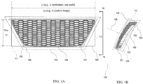
- two of the finest variable resolution VR regions e.g., VR10 103 and VR11 102 may be applied to enclose the vehicle's grille 101, as illustrated schematically in FIGS. 1A and 1B .
- VR11 102 is closer to the grille 101 than VR10 103 in the illustrated implementation. As such, VR11 102 more closely envelops the grille 101 than does VR10 103.
- Each of VR11 102 and VR10 103 approximates the overall shape of the grille, without regard to the narrow gaps/holes 104 in it).
- meshing size used in VR11 is 1 mm and mesh sizing in VR10 is 2mm.
- VR11 enclosing the grille may no longer be needed (e.g., if the opening size is larger than 16 mm).
- Variable resolution regions VR10 103 and VR11 102 are shown as enclosing the vehicle's grille 101 in FIGS. 1A and 1B .
- VR10 102 which may have 1mm mesh sizing, is closer to the grille 101 than VR11 102, which may have 2mm mesh sizing.
- the grille 101 represented in the illustrated image (which may appear on a computer screen as a rendering of a CAD or mesh file) has a rigid body that is contoured to define an outer rim 108 that surrounds an internal portion with structures that define a honeycomb pattern of substantially uniform gaps/holes 104 that extend through the grille 101 (e.g., from a front face of the grille, which is visible in FIG. 1A , to a rear face of the grille, which is opposite the front face).
- every gap/hole 104 in the internal portion of the illustrated grille 101 is the same as or similar to all the other gaps/holes 104 in the internal portion, except at the edges (top, bottom, and sides) of the internal portion, where some of the gaps/holes 104 are cut off by the outer rim 108.
- a front surface of the internal portion of the grille 101 extends forward a bit from a forward edge of the outer rim 108. From an aesthetic perspective, the visual effect produced by the pattern may be pleasing or appealing to the viewer. From a functional perspective, the pattern provides air flow communication channels through the grille into a vehicle's underhood region, for example.
- This air flow typically helps to remove the heat out of the vehicle when operating and particularly while the vehicle is in motion under the influence of the engine or electric motors.
- the narrow gaps/holes 104 in the grille 101 allow for air to flow from outside the vehicle, through the grille 100 in a roughly horizontal direction (e.g., left to right in FIG. 1B ), and into the vehicle's underhood region.
- a bounding box is a virtual box that surrounds and defines the minimum or smallest bounding or enclosing box for the set of points that make up the grille model.
- Bounding boxes can be aligned axially (e.g., with edges that lie parallel to cartesian coordinate axes arranged parallel to and perpendicular to the direction of gravity, for example).
- a bounding box can be oriented relative to the grille 101 design in a manner (as shown), which would minimize the internal volume of the bounding box.
- the illustrated OBB 105 defines the minimum or smallest bounding or enclosing box for the set of points that make up the car model with the smallest volume within which all the points lie.
- the illustrated OBB 105 is a square cuboid with a front surface that contacts a frontmost point of the modeled grille 101, a rear surface that contacts a rearmost point of the modeled grille 101, side surfaces that respectively contact furthest points on either side of the modeled grille 101, a bottom surface that contacts a lowest point of the modeled grille 101, and a top surface that contacts a highest point on the modeled grille 101.
- one or more of the bounding box surfaces may contact more than one point on the modeled grille 101 if those points are all lie in the same plane and include the furthest point in that dimension.
- Dimensions of the OBB 105 implicitly define an overall length, height, and width of the modeled grille 101.
- the viewing vector is a vector that originates outside (and in front of) the modeled grille 101, is directed toward a front face of the grille 101 and is oriented perpendicular to a front face 107 of the OBB 105. Viewing the modeled grille 101 from the viewing vector 106 enhances the likelihood that one would see as much as possible through the gaps/holes 104 in the grille 101 given the depth (e.g., dimension into the page in FIG. 1A ) and contours of the structure that defines the gaps/holes 104.
- opening sizes in grilles may vary and VR assignment based on size opening may be subject to an engineer's subjective and sometimes imprecise and inconsistent judgement to determine which size should be used for determining VR assignments.
- manually measuring the size could introduce human errors as picking two points for distance measurements can be somewhat subjective.
- manual measurement of a size and then manual assignment of the VR region may not be feasible or practical (from a speed or efficiency perspective) in an automated workflow in which manual inputs are desirably minimized.
- an automated method to accurately measure the opening size is needed to facilitate simulation workflow automation and to reduce uncertainties from any human factors.
- This goal could be possibly achieved by analyzing the 3D geometry, identifying possible gaps and then attempting to calculate the size of the gap. For example, rays could be emitted from centroids of all triangles if the geometry has been triangulated and gap sizes can be determined by measuring the traveling distances of these rays. Although algorithms such as octree could be used to improve the performance of this ray-tracing method, determining if the returned distances belong to the target gap/opening is still challenging. Another method may be to identify two sets of points from two objects and then utilize Delaunay tetrahedralization to calculate the gap between these two objects or two points. ( See, e.g., S. Goswami, G.
- Burenkov 2022, "Detection of gaps between objects in computer added design defined geometries ", US Patent Application Serial No. 16/504,599 .)
- user inputs are usually needed to define thresholds of gap distance and the angle formed by these two objects, which is less than desirable for simulation workflow automation purposes.
- grille openings/holes can vary across vehicle models/designs.
- grille openings in different vehicle models/designs can be rectangular, hexagonal, and circular and so on.
- the opening size may look smaller visually when the viewing angle is parallel to the vehicle moving direction. This introduces challenges when analyzing the grille opening size use any image processing techniques directly. Implementations of the systems and techniques disclosed herein address and overcome these technical issues.
- implementations of the systems and techniques disclosed herein may be able to identify the contour of the openings and determine overall opening size in the presence of noise, and/or handle grilles with varied orientations and designs.
- the systems and techniques disclosed herein may be integrated into automated computational fluid dynamics (CFD) simulation workflows (e.g., implemented by computer software executing on a computer to perform CFD simulation) to automatically assess and/or determine a value to be used as an opening size for a vehicle grille so that correct VR regions can be assigned to the grille region in order to optimizes simulation resources in the CFD simulation.
- CFD computational fluid dynamics
- the systems and techniques disclosed herein may be utilized to detect the opening size of any equipment or device which is designed for ventilation.
- FIG. 8 is a schematic representation of an exemplary implementation of a computer 1000 that is configured to automatically determine a value representing opening size for a vehicle's grille based on a computer-based representation of the grille's geometry. In some implementations, this determination facilitates or enables automatic assignment (e.g., by the computer 1000) of one or more three-dimensional (3D) variable resolution (VR) regions at or near the grille to be used in a computer-based simulation (e.g., CFD) involving the grille so as to appropriately balance the competing interests of precision and efficiency.
- 3D three-dimensional
- VR variable resolution
- the illustrated computer 1000 has a processor 1002, computer-based memory 1004, computer-based storage 1006, a network interface 1007, an input/output device interface 1010, and an internal bus 1012 that serves as an interconnect between the components of the computer 1000.
- the bus 1012 acts as a communication medium over which the various components of the computer 1000 can communicate and interact with one another.
- the processor 1002 is configured to perform the various computer-based functionalities disclosed herein as well as other supporting functionalities not explicitly disclosed herein. Some of the computer-based functionalities that the processor 1002 performs are those functionalities disclosed herein as being specifically attributable to the computer 1000 (or to processor 1002). In some implementations, the processor 1002 performs these and other functionalities by executing computer-readable instructions stored on a computer-readable medium (e.g., memory 1004 and/or storage 1006). In various implementations, some of the processor functionalities may be performed with reference to data stored in one or more of these computer-readable media and/or received from some external source (e.g., from an I/O device through the I/O device interface 1010 and/or from an external network via the network interface 1007).
- the processor 1002 in the illustrated implementation is represented as a single hardware component at a single node on a network. In various implementations, however, the processor 1002 may be distributed across multiple hardware components at different physical and network locations / nodes.
- the computer 1000 has both volatile and non-volatile memory / storage capabilities (e.g., in memory 1004).
- memory 1004 is configured to host the computer's operating system 1020 as well as executable software 1008.
- memory 1004 serves as a computer-readable medium storing computer-readable instructions that, when executed by the processor 1002, cause the processor 1002 to perform one or more of the computer-based functionalities disclosed herein.
- memory 1004 stores computer software that enables the computer 1000 to perform various functionalities disclosed herein including, for example, determining a value to represent opening size for a vehicle's grille based on a computer-based representation of the grille's geometry (e.g., stored as a CAD file in computer memory), and/or automatically identifying and assigning one or more three-dimensional (3D) variable resolution (VR) regions (based on the determined value for opening size) at or near the grille to be used in a computer-based simulation involving the grille, and/or conducting a computer-based simulation involving the grille utilizing one or more of the assigned 3D VR regions at or near the grille.
- 3D three-dimensional
- this computer software may be a stand-alone component, but in other implementations, this computer software may be integrated into, and/or be designed to be and operable to be utilized in connection with, another software program stored in memory 1004 to facilitate and perform computer-based simulations that utilize either the computed values for opening size, VR region assignments (based on the computed opening sizes), or both in running simulations based on a grille's geometry.
- the aforementioned computer software may be integrated into PowerFLOW ® simulation software available from Dassault Systèmes Simulia Corp.
- PowerFLOW ® simulation software provides unique solutions for computational simulation of fluid-flow problems. It is suitable for a wide range of applications, whether simulating transient or steady-state flows.
- PowerFLOW offers a wide range of modeling and analysis capabilities, including aerodynamics simulations, thermal simulations (including, e.g., convection, conduction, radiation, and heat exchangers), and aeroacoustics simulations.
- PowerFLOW ® simulation software is able to simulate fluid-flow design problems in such industries as automotive and other ground transportation, aerospace, petroleum, building design and architecture/engineering/construction (AEC), heating, ventilating, and air conditioning (HVAC), and electronics.
- Automotive applications include, for example, full car external aerodynamics for drag and lift, underbody design, noise source identification or aeroacoustics for side mirror, antenna, glass offset and detail design, wind tunnel design and validation, intake ports, manifolds, heating, and air conditioning ducts, under hood cooling, filter design, and windshield wiper design, etc.
- a program such as PowerFLOW ® simulation software may have the ability, when executed by computer, to automatically determine a value representing opening size in a vehicle grille, to facilitate and/or automatically assign three-dimensional (3D) variable resolution (VR) regions at or near the grille (e.g., for computer-based simulation purposes), and/or to run simulation(s) of the grille based on the assigned 3D VR region(s).
- 3D three-dimensional
- VR variable resolution
- the computer 1000 in the illustrated implementation, also has a storage device 1006, which can be virtually any form of computer-based storage device or component.
- FIG. 2 is a flowchart representing an exemplary implementation of a process for determining a value representing size of the openings in a grille based on a virtual, three-dimensional, computer-based representation of the grille including its geometry.
- this value can be utilized to facilitate and/or enable automatic, or at least simplified, assignment of one or more three-dimensional (3D) variable resolution regions at or near the grille for use in connection with simulating the grille in a computer-based environment (e.g., from a computational fluid dynamics perspective).
- the process represented by the illustrated flowchart is implemented within a computer-based environment, such as on computer 1000 of FIG. 8 , with the illustrated processing steps being performed by or with the assistance or involvement of processor 1002.
- the process includes (at 201) importing a three dimensional (3D) grille geometry.
- this importing step includes importing a computer-based representation of the 3D grille geometry (e.g., from one application to another).
- the source (or origin) application in this case may be, for example, the software application where the computer representation of the 3D grille geometry was created and/or stored.
- This may be a computer-aided design (CAD) application, such as SOLIDWORKS ® CAD software, available from Dassault Systèmes.
- CAD computer-aided design
- the destination application in this case would be the software application where the processes otherwise represented in FIG.
- the destination application may be PowerFLOW ® simulation software, also available from Dassault Systèmes, adapted to include the functionalities represented in FIG. 2 and described herein.
- the destination application may include a geometry tool or a geometry viewer that facilitates viewing a visual representation of the 3D grille on a computer screen (e.g., connected to 1010 in FIG. 1 ).
- the 3D grille geometry may be contained in a CAD or mesh file imported from a geometry program, for example at step 201.
- the importation process (at 102) is performed by a computer (e.g., 1000) automatically. In some implementations, the importation process (at 102) is performed in response to a human user selecting an import option (e.g., at a user interface of computer 1000) or taking some other step or combination of steps to initiate importation. In an exemplary implementation, the importation process will result in importing data representative of the grille 101 design shown in FIGS. 1A and 1B . The data that gets imported (at step 201), however, typically will not include information representing the OBB 105, the viewing vector 106, or any of the 3D VR regions 102, 103. In an exemplary implementation, the data representative of the grille 101 geometry shown in FIGS. 1A and 1B will be imported from, or in the form of, a CAD file.
- the computer 1000 calculates an oriented bounding box (OBB) 105 for the imported grille (e.g., 101) geometry.
- This step involves determining virtual parameters for the OBB 105, relative to the imported grille 101 design, to fully define the OBB 105, as shown in FIGS. 1A and 1B .
- the OBB 105 typically is generated directly from the imported grille (e.g., 101) geometry.
- the computer 1000 stores computer executable instructions that, when executed by the computer processor 1002, causes the computer processor 1002 to automatically generate the OBB 105 parameters (and, optionally, a visual representation of the OBB 105, e.g., as shown in FIGS. 1A and 1B ) based on the imported grille (e.g., 101) geometry.
- the computer 1000 calls on this OBB-generating functionality automatically (e.g., in response to the modeled grille (e.g., 101) being imported at 201).
- the computer 1000 calls on the OBB-generating functionality in response to an external prompt from a human user, for example.
- the computer 1000 may be configured to present a user-selectable option at its user interface, the selection of which, by a human user, causes the computer 1000 to call on the OBB-generating functionality to then automatically generate the OBB 105 based on the imported grille geometry.
- the computer 1000 may apply a rotating calipers algorithm to the imported grille geometry data set.
- This rotating calipers algorithm may be based on an approach described in an article by Joseph O'Rourke in 1985 at pages 183-199 of the International Journal of Computer & Information Sciences, entitled Finding Minimal Enclosing Boxes .
- This approach is based on lemmas characterizing the minimum enclosing box as follows: 1) there must exist two neighboring faces of the smallest-volume enclosing box which both contain an edge of a convex hull of the point set (this criterion may be satisfied by a single convex hull edge collinear with an edge of the box, or by two distinct hull edges lying in adjacent box faces); and 2) the other four faces need only contain a point of the convex hull (the points which they contain need not be distinct: e.g., a single hull point lying in the corner of the box already satisfies three of these four criteria). ( See also Shamos, M., 1978. "Computational Geometry,” Yale University. pp. 76-81 ).
- the OBB 105 may be stored as data (e.g., in computer memory 1004).
- the computer 1000 may be configured to produce a visual representation of the OBB 105 on a computer display screen (e.g., coupled to 1010) and that visual representation may appear like the visual representation of the OBB 105 in FIGS. 1A and/or 1B.
- the computer 1000 may be configured to present a visual representation of the OBB 105 on its display.
- the visual representation of the OBB 105 is presented along with an image of the grille 101 geometry associated with the OBB 105.
- various other information e.g., dimensions such as length, height, and/or width
- location information of the corner nodes of the OBB 105 may be displayed or accessible to the user through the user interface on the display.
- the OBB 105 is a six-sided, 3D box, where each side (or face) is perpendicular to any adjacent sides (or faces).
- FIGS. 1A and 1B An example of this is shown in FIGS. 1A and 1B , where the OBB 105 is 3D and has six sides (or faces) - a front face 107, a rear face 109, a right side face 111, a left side face 113, a top face 115, and a bottom face 117.
- Each of these faces 107-117 is perpendicular to an adjacent one of the faces.
- the front face 107 of the OBB 105 is perpendicular to adjacent top face 115, adjacent bottom face 117, and the adjacent side faces 111, 113.
- the computer 1000 calculates the initial viewing vector 106.
- the computer 1000 calculates the initial viewing vector 106 using the grille's O+BB 105 information.
- the computer 1000 may calculate the initial viewing vector 106 using the grille's OBB 105 information. For example, most of the time, the grille under consideration is a front grille, and the vehicle is, by typical convention, arranged (e.g., as shown) always along X direction. So, the computer 1000 may, in those implementations, simply use +X direction as the viewing direction.
- geometry tools typically have a "zoom to fit" function built-in.
- the computer 1000 can be made to set +X direction as the viewing direction and use that zoom to fit to create a perfect view of the grille. Moreover, in certain implementations, once the computer 10000 has obtained the OBB information, the system can designate the center of the OBB as a starting point, and the direction of the vector will be perpendicular to the OBB's front face.
- the initial viewing vector 106 is perpendicular to and directed towards the front face of OBB 105 to ensure that the chance for openings to be visible (and able to be seen through) in the starting image taken in step 205 is relatively high.
- the computer 1000 may be configured to present a visual representation of the initial viewing vector 106.
- the visual representation of the initial viewing vector 106 may appear in the same way that the initial viewing vector 106 appears in FIG. 1B , namely with the initial viewing vector 106 appearing along with an image of the grille 101 geometry and the associated OBB 105.
- various other information e.g., dimensions such as length, height, and/or width
- location information of the corner nodes of the OBB 105 may be displayed or accessible to the user through the user interface on the display.
- the computer 1000 creates a spatial calibration box 302.
- the relationship (or ratio) between the pixel domain (e.g., the image of the grille) and the physical domain (e.g., the real world version of the modeled grille) needs to be established.
- This process is called spatial calibration, and the relationship / ratio sought after in this regard is represented by a conversion ratio or calibration factor (and may be referred to as the pixel-to-real-distance ratio).
- This calibration factor may change if, for example, the image of the object is rotated (e.g., on screen) due to the change of visible pseudo size in the unit of pixel as displayed in the image.
- the spatial calibration box 302 may be created.
- the spatial calibration box 302 is as shown in FIG. 3A-3C and is a 3D box with a very small thickness (e.g., 1 millimeter) or a two-dimensional (2D) square.
- the computer 1000 sets the height (H SCB ) and width (W SCB ) of the spatial calibration box 302 equal to the height (H OBB ) of the OBB 105.
- the computer 1000 locates a geometric center of the spatial calibration box 302 to the left (or right) of the image of the grille 301 geometry (as shown in FIGS.
- FIG. 3A is a view showing an exemplary spatial calibration box 302 next to a front view image of a grille 301 geometry that may have been generated from grille geometry data imported at 201.
- Grille geometry 301 in FIGS. 3A-3C is similar to grille geometry 101 view in FIG. 1A .
- Two of the vertices of the spatial calibration box 302 are marked as 312 and 313 in FIG. 3A .
- Also shown are two axes of rotation: a horizontal axis of rotation 304, and a vertical axis of rotation 306. Each of these axes 304, 306 passes through the image of the modelled grille 301 (e.g., through the geometrical center of the image of the modelled grille 301).
- FIG. 3B shows an image 308 that is similar to the image in FIG. 3A in that it shows an image of the spatial calibration box 302 next to a front view image of the grille 301 geometry.
- FIG. 3C shows an image 309 that is similar to the image in FIG. 3A in that it shows an image of the spatial calibration box 302 next to a front view image of the grille 301 geometry.
- the images 308 and 309 are example ones generated from backward (clockwise) and forward (counter-clockwise) rotations (about horizontal axis 304) of the image 307 in FIG. 1 .
- the view of the grille 301 geometry and the openings in the grille 301 appear different - in size and shape as the image is rotated about the horizontal axis, as indicated.
- the computer 1000 is configured to produce a sequence of images, such as those represented in FIG. 3A, 3B, and 3C by rotating the starting image (e.g., about the horizontal axis 304) either backwards or forwards or both.
- the computer 1000 may be configured to take a screenshot of the image at each angle of rotation, including whatever the initial angle (which may be designated as 0 degrees, arbitrarily).
- the screenshots may be saved (e.g., in memory 1004) as they are created. This produces a series of images of the grille 301 geometry and the spatial calibration box 302 next to the grille 301 geometry at different angles of rotation (about a common axis, e.g., the horizontal axis 304).
- the computer 1000 (at 205) takes a screenshot of the grille 301 and the spatial calibration box 302 with them present at the same time on the display screen and with a rotation angle of zero degrees.
- This rotation angle zero degrees
- the viewing angle used for generating this screenshot is determined by the initial viewing vector 106.
- the image thus captured may be designated as a first or primary image 307 in a sequence of images showing the grille 301 and the spatial calibration box 302 at different rotational angles (rotated about the horizontal axis 304).
- the computer 1000 rotates the image of the grille 301 geometry and the spatial calibration box 302. In one implementation, this rotation occurs about the horizontal axis 304. However, in other implementations, the rotation occurs about the vertical axis 306 instead.
- the direction of rotation can be forward (represented by the curved arrow around the horizontal axis 304 in FIG. 3A ) or backwards (opposite the curved arrow around the horizontal axis 304 in FIG. 3A ).
- the angular amount by which the computer rotates the image (at 206) can vary. In various implementations, the angle is one degree or less, two degrees or less, three degrees or less, four degrees or less, five degrees or less, ten degrees or less, etc.
- the rotation changes the visual appearance of the image from what it appears like in FIG. 3A (307) to what it appears like in FIG. 3C (309).
- its appearance including how much of the openings in the grille can be seen through
- the appearance of the grille's thickness increases from 314 (in view 307 of FIG. 3A ) to 315 (309 in FIG. 3C ) as the image of the grille 301 geometry is rotated forward (about horizontal axis 304).
- the computer 1000 (at 207) takes a new screenshot of the new view (309).
- the computer 1000 typically stores the new screenshot in memory (e.g., 1004) together with the original screenshot (taken and saved at 205).
- steps 206 and 207 are repeated multiple times with the same image with screenshots taken at different angles of rotation to produce a sequence of multiple different images showing the same grille 301 geometry from different perspectives / viewing angles.
- Each of these screenshots may be stored together in memory (e.g., 1004).
- the different perspectives / viewing angles results from the computer 1000 rotating the image forward for each screenshot a little farther than the previous screenshot.
- the different perspectives / viewing angles results from the computer 1000 rotating the image backward for each screenshot a little farther than the previous screenshot.
- the different perspectives / viewing angles may result from the computer 1000 rotating the image forward and backward different amounts relative to the viewing angle and perspective of the original screenshot (taken and saved at 205).
- the foregoing approach can be helpful, for example, because depending on the specific grille design and its orientation, the image 307 generated using the initial viewing vector 106 may not be best image to analyze the opening size.
- One reason for this is that the opening holes might be blocked (e.g., by surrounding structures) leading to misleadingly small openings being displayed in the image. Significant errors may be introduced if such an image (e.g., with misleadingly small opening sizes displayed) is used to calculate opening size(s).
- opening sizes are measured manually (e.g., by an engineer in the real world), the engineer may rotate the real world grille to find the best viewing angle before actually measuring the opening size(s).
- the computer 1000 rotates the image of the grille 301 geometry -- pivoted at its geometric center about its horizontal axis 304 in step 206.
- the camera viewing angle and location i.e., the perspective from which the screenshots are taken at 207) is kept unchanged during the geometry rotating process.
- a screenshot containing the grille 301 and calibration box 302 is taken at every ⁇ ° rotation angle (at 207).
- the value of ⁇ may be optimized to balance the performance and accuracy.
- the rotation may happen in clockwise and counter-clockwise directions or both sequentially depending, for example, on at what angle the target image is found.
- images 308 and 309 are example ones generated from backward (clockwise) and forward (counter-clockwise) rotations.
- the computer 1000 identifies which one of those images has the largest opening size(s). This process is discussed further below. If none of the images can be identified as having the largest opening size(s) (at 208), then, according to the illustrated flowchart, the computer 1000 progresses to step 209 and rotates the image of the grille geometry (e.g., initial image 307) along the vertical axis 206 (at 209), taking a screenshot 207 at every ⁇ ° rotation angle (207), to produce a new series of images that show the grille 301 geometry alongside the spatial calibration box 302 at different angles of rotation about vertical axis 306.
- the image of the grille geometry e.g., initial image 307 along the vertical axis 206 (at 209), taking a screenshot 207 at every ⁇ ° rotation angle (207)
- the computer 1000 After producing this new set of images, the computer 1000 returns to step 208 and attempts to find the image with the maximum opening size - this time among the new collection of screenshot images - showing the same grille geometry from different viewing angles and perspectives - now, rotated about the vertical axis 206 instead of the horizontal axis 204.
- the computer saves or flags that image with a designation in memory indicating that characteristic.
- the computer 1000 calculates a calibration factor (or pixel-to-real-distance ratio) for the image that was determined (at 208) as the one having the maximum opening size. Since the physical height of the spatial calibration box 302 is known already (and stored in memory, e.g., 1004) from step 204 when it was created, only its height in the unit of pixel is needed to be determined. In one embodiment, this may be calculated by a process that involves casting rays (310, 311) from and near the upper corner of the display screen in a vertically downward direction ( see rays 310 in the image 307 in FIG.
- the corners from which these rays (310, 311) are cast are the corners on the spatial calibration side of the display screen (i.e., the side of the grille 301 geometry where the spatial calibration box 302 is located).
- one ray at a time may be cast from the upper edge of the image 307 and from the lower edge of the image 307.
- the first of each ray cast the upper edge and the lower edge may be closest to the leftmost edge of the image 307 and each subsequent ray may be cast originating at points on the upper and lower edges that are some number (one or more) pixels next to the previous ray -- towards the spatial calibration box 302.
- multiple rays may be cast simultaneously from the upper edge of the image 307 in a downward direction and simultaneously from the lower edge of the image 307 in an upper direction.
- the computer 1000 may conclude that no portion of the spatial calibration box 302 lies along the path traversed by that cast ray. For example, the leftmost rays (downward cast and upward cast) in FIG. 3A would traverse the entirety of the image 307 without reaching a darkened pixel. When that happens, the computer 1000 concludes that no portion of the spatial calibration box 302 lies along the paths traversed by those leftmost rays.
- the computer 1000 may conclude that that darkened pixel corresponds to (and forms a part of) the spatial calibration box 302.
- the computer 1000 records (e.g., in memory 1004), the traveling distances of the cast rays (e.g., one from each group of cast rays 310 and 311) when the rays hit any darkened pixel (e.g., a pixel having a black color), indicating that the pixel belongs to the calibration box 302.
- the traveling distance is recorded in units of pixels.
- the casting process stops when at least one ray from each group of rays 310, 311 hits one black pixel. The coordinates of these two hit points in the unit of pixel are returned (and stored, e.g., in memory 1004).
- the computer 1000 is able to (and does) determine the height of the spatial calibration box 302 in pixel as being equals the vertical distance between these two vertices. Since the calibration box 302 is a square in a two-dimensional (2D) domain, its location information (e.g., the coordinates of its four vertices) in the image is known by the computer 1000. Thus, the computer 1000 is able to (and does) identify the calibration factor by dividing the physical height of the spatial calibration box (e.g., in millimeters) by its height in pixels. The units of the calibration factor then may be mm/pixel (mm is chosen for representative purpose, other physical units could be chosen) representing the physical dimension in the unit of mm per pixel.
- the pixel height of the calibration box 302 can be obtained by first extracting the pixel information representing the four edges of the box, and then either finding one pair of parallel point sets to calculate the distance between these two point sets or finding the maximum distance among all edge points to get the diagonal distance and then using Pythagorean theorem to calculate the box height.
- the computer 1000 in such implementations, would perform these calculations. Since the grille 301 and the calibration box 302 are present in the image 307 together, there is some work needed to be done in order to extract the edge information of the calibration box 302.
- One method is to hide grille 301 and take another screenshot with the box alone without changing the viewing vector and then perform an edge detection (e.g., using ray casting, as described above) to extract calibration box 302's edge information.
- Another method is to assign a color to the calibration box 302 geometry in the view and use the RGB (red, green, blue) values of that color to identify the calibration box 302.
- the geometry viewing tool offers an option to assign an appearing color for the geometry. For example, once a box is loaded into a geometry tool, the user can set the color of that box to be yellow or red instead of the default color displayed to the user (usually gray). Say a user sets red for the calibration box. Then the computer 1000 may check the color or RGB values of given image which contains this box and the grille. Since the computer 1000 is able to recognize that the box at issue is red, then the computer 1000 can know that / designate any red pixels as belonging to box. Thus, the computer 1000 in this regard can identify the location of calibration box.
- the computer 1000 stops the rotation-screenshot-taking process after a predefined total number of images has been acquired.
- This predefined number may be stored in memory (e.g., 1004) and may, in some instances, be user-specified. In such implementations, the process terminates when this number is reached.
- the computer 1000 typically stores all collected images in memory (e.g., 1004).
- the computer 1000 finds which of the collected image has the maximum (or largest) visible opening size among the images that have been collected.
- the collected images are categorized into three groups, the initial image taken at 0° rotation angle, the image set created from backward rotation, and the image set created from forward rotation.
- each hole has an area of Ai.
- the computer 1000 is configured to sum all areas of the holes and get the total opening area A.
- the computer 1000 further determines an area A, denoted the maximum opening area, which is equal to the max of all Ai among all images.
- the image with the maximum opening area displayed is the target image as it represents the largest opening size.
- the computer 1000 computes the total opening area of each image starting from the initial image and then sweeps through the backward rotation image set in order of increasing rotation angle, for example. In most instances, the value computed for total opening area changes (e.g., increases or decreases) from image to image as the computer progresses from the initial image through the backward rotation image set. In a typical implementation, the computer 1000 stops the sweeping process if/when the total opening area computed for a particular image is found to be declining (i.e., less than the computed total opening area for the immediately prior image) considered in the sweeping process. This image (i.e., the image in the sequence immediately prior to the image that had the declining total opening area) is selected, and designated in memory 1004, as a temporary target image.
- This image i.e., the image in the sequence immediately prior to the image that had the declining total opening area
- the computer 1000 in this example sweeps the forward rotation image set in order of increasing rotation angle, to determine whether there are any images whose total opening area is larger than the previously designated temporary target image. Similarly, the computer 1000 stops the sweeping process (of forward rotation images) if/when the value is found to be declining from one image to the next image.
- the computer 1000 designates (in memory 1004) the temporary target as a final target image (i.e., the image, among all captured images, that has the largest opening area). If the sweep of forward rotation images reveals any images whose total opening area is larger than the previously designated temporary target image (found by scanning the reverse rotation images), then the computer 1000 designates (in memory 1004) as the final target image that image in the sequence of forward rotation images that came immediately prior to the image that showed a declining total opening area.
- the computer 1000 designates (in memory 1004) the initial image as the final target image.
- the final target image is identified by the computer 1000 once this process has been completed.
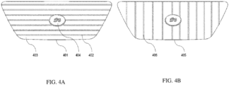
- the process described above may work well for a grille with meshed or honeycomb designs similar to grille 301 or for a grille similar to 401 with horizontal bar designs.
- the horizontal bar 402 in the grille 401 or the hexagonal holes in the grille 301) will create blockage of viewing the holes (e.g., 403) in the grille.
- obvious changes are apparent (and able to be identified using the foregoing methods) so the rotating process could be terminated even with the presence of noisy objects such as the logo 404.
- the computer 1000 may introduce an extra step(s) 209 to rotate the grille along its vertical axis 306 if no target image is found in step 208.
- the image sweeping process in step 208 is repeated for these new sets of images (created by screenshotting an initial view, a series of views of the grille rotated to the left, and a series of views of the grille rotated to the right).
- the computer 1000 stops the rotation-screenshot-taking process by dynamically analyzing the generated image at each angle of ⁇ and only continuing to generate a new image after the total opening area of current image is computed. This process still follows the sequence of initial-backward-forward screenshot captures. Compared to the method used in the first embodiment described above, this method may end up analyzing fewer or the same number of images depending on the specific grille design involved.
- the computer 1000 calculates the total opening area in step 208 in a less computationally intensive manner.
- the computer creates an image as or converts an image to a binary image that only consists of two colors or distinct appearances (e.g., white and black).
- the computer 1000 in an exemplary implementation, directly generates a binary image in step 205 when the screenshot is taken by setting the background color of the geometry tool or viewer to be white and the color of grille geometry to be black.
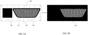
- FIG. 5A An exemplary appearance of a binary image of a grille 501 (created at step 205), with the background color of the geometry tool or viewer set to be white and the color of grille 501 geometry to be black, is shown as part of the image 502 in FIG. 5A . Also included in image 502 is a view of a spatial calibration box 505 next to the grille 501 geometry.
- the image 502 shown in FIG. 5A cannot be directly used for the total opening area calculation by the computer 1000 because the space 503 around the grille 501 and the calibration box 505 has the color of white (like the openings in the grille 501).
- the change of the total area of the space 503 is unpredictable due to the unknown shape of the input grille 501 (the phrase "input grille” here relates to the grille data loaded into the program or geometry viewer).
- the computer 1000 colors the space 503 black to produce the image 506 in FIG. 5B , in which only the holes / openings in the grille 501 are white.
- the rest of the image 506, as from the white holes / openings, is black.
- the computer 1000 may produce the image 506 in FIG. 5B from the image 502 in FIG. 5A .
- the computer 1000 automates the foregoing space coloring process by utilizing a ray casting method and shooting rays 504 (see, e.g., FIG. 5A ) from all four sides of the image 502 in a horizontal or vertical inward direction.
- the computer 1000 examines the color of each pixel that each ray 504 visits and updates the color of that pixel to black if the original color of that pixel was white.
- Each ray 504 stops when it reaches a pixel that already was black (when the ray reached it). In some instances, reaching the already-black pixel represents the fact that the ray at issue may have reached a boundary of the grille and, therefore, can (and does) stop.
- the color of the calibration box 505 is also black which would fail the algorithm if not treated specially. For example, if the rays 504 coming off the left side of the image 502 simply stopped when they reached the left edge of the spatial calibration box 505, then portions of the white space 503 between the spatial calibration box 505 and the grille 501 would not get turned black, and subsequent calculations of opening area would be compromised.
- One way of addressing this challenge is as follows.
- the computer 1000 Since the coordinate information of four vertices of the calibration box 505 has been obtained previously by the computer 1000 (and stored in memory 1004) when the calibration factor was calculated (at 210), the computer 1000 simply does not update the colors for the pixels that the rays reach that are within the spatial calibration box 505 zone (i.e., within the space outlined by a rectangle having corners at the vertices) and resume updating the colors of pixels (from white to black) once a ray reaches pixels that are outside of that zone. Also, even though the pixels are black (inside the spatial calibration box zone), the computer allows the rays to continue moving through the spatial calibration box zone, instead of stopping them, which the computer otherwise does when a ray reaches a black pixel. Once this process is completed, all spaces surrounding the grille 501 and the calibration box 505 will have been colored black as shown in image 506.
- Black and white coloring are described herein as being used in a particular manner. In other implementations, the coloring can be reversed from what was just described (and represented in FIGS. 5A and 5B ). In still other implementations, different colors, shading, patterns, etc. may be utilized instead of simply black and white coloring.
- the computer 1000 calculates the total number of white pixels in the image 506 of FIG. 5B .
- the computer 1000 designates this value (total number of white pixels in the image 506) as the total opening area in the image 506.
- the computer may accomplish this task (of counting the total number of white pixels).
- the computer 1000 utilizes the function findNonZero in the OpenCV ® library to compute the total counts of the white pixels in image 506. ( See, e.g., Bradski, G., 2000. The OpenCV Library. Dr. Dobb's Journal of Software Tools ).
- the computer 1000 calculates a calibration factor (or pixel-to-real distance ratio) for this image in step 210.
- the computer 1000 extracts the edges of all objects in the target image (at 211).
- the computer 1000 may utilize a Canny edge detector to obtain the edge information.
- Canny edge detectors may implement computational approaches to edge detection such as described, for example, in Canny, J.
- An exemplary Canny edge detection algorithm involves these steps: 1) apply a Gaussian filter to smooth the image in order to remove the noise, 2) find the intensity gradients of the image, 3) apply gradient magnitude thresholding or lower bound cut-off suppression to get rid of spurious response to edge detection, 4) apply double threshold to determine potential edges, 5) track edge by hysteresis: finalize the detection of edges by suppressing all the other edges that are weak and not connected to strong edges.
- edge detection produces a binary image where edges from the target image are represented as ones (and may be shown in an image as black pixels) and anything other than an edge is represented as zeros (and may be shown in an image as a white pixel). Variations in the edge detection process are possible.
- the computer 1000 typically saves the edge information extracted at 210 (in memory 1004) and feeds the extracted edge information into step 212 of the illustrated process.
- the computer 1000 finds all the contours in the target image, represented by the extracted edge information, and calculates their areas. Contours are essentially curves joining continuous points (along a boundary) having same color or intensity. Contours can be a useful tool for shape analysis and object detection and recognition.
- the computer 1000 utilizes the findContours function in OpenCV ® ( see, e.g., Bradski, G., 2000. The OpenCV Library. Dr. Dobb's Journal of Software Tools ) to perform contour calculations based on the extracted edge information, for example. This function typically retrieves contours from the binary image form of the target image produced by the edge extraction process discussed above.
- the computer 1000 uses an algorithm for finding contours based on the description provided by Satoshi Suzuki, et al. in an article entitled Topological structural analysis of digitized binary images by border following, in Computer Vision, Graphics, and Image Processing, 30(1):32-46, 1985 ).
- the computer 1000 typically saves the contours generated (at 212) in memory 1004.
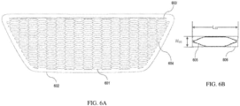
- FIG. 6A shows an example of an image produced by finding the contours from a set of extracted edge information of a target image.
- the image in FIG. 6A shows the grille of the target image with all edges of the grille (e.g., interfaces between solid and space) shown with dark lines and all other space shown in white.
- the dark lines in the image provide an outline of all edges from the target image of the grille.
- the computer 1000 is configured to produce the image shown in FIG. 6A on its display, which may be connected to 1010.
- These captured contours are raw and not well suited for use to directly calculate overall grill opening size at least because they include noisy contours such as 602, 603, and 604 in addition to the target contours 601.
- the target contours 610 in this regard correspond to openings in the grille that are full size - i.e., not truncated by the end of the pattern of openings at the sides, top, or bottom of the grille.
- Contour 602 is a contour that surrounds all other contours.
- Contour 603 is a contour that extends across the top of the space within contour 603.
- Contours 604 correspond to the openings in the grille that are at the sides, top, or bottom of the pattern of openings in the grille and, therefore, are truncated so that they are smaller, sometimes significantly smaller, than the full size (non-truncated) target contours 610 that appear inward of the sides, top, and bottom of the pattern of openings in the grille.
- the areas of all raw contours are calculated in step 212.
- the areas may be calculated utilizing the function minAreaRect from OpenCV ® . This creates a list of area values of all raw contours. In some implementations, this list will identify calculated areas for the space within contours 601, as well as all the space within contours 602, 603, 604, and any other contours that may have been identified by the computer 1000 (at 212).
- the computer 1000 rejects outliers (e.g., contours 602, 603, and 604) based on their area values (as calculated in 212) and obtains the list of all candidate contours. In some implementations, the computer 1000 performs this step (of rejecting outliers) according to the following exemplary process.
- outliers e.g., contours 602, 603, and 604
- the computer 1000 performs this step (of rejecting outliers) according to the following exemplary process.
- the computer 1000 produces (and stores in memory 1004) a listing containing these calculated deviation values A di , with one deviation value for each respective one of the area values listed in the raw contour area listing.
- the computer 1000 calculates a median value of the deviation values in the listing of calculated deviation values, which may be denoted (and stored in memory 1004) as A d .
- a ni A di A d ⁇
- a ni the normalized area deviation value.
- a ni is set to be zero when A d is detected to be zero.
- the computer 1000 chooses an optimized non-dimensional factor s (an empirical value based on testing) and removes any element of the raw contour area list whose A ni value (or normalized area deviation value) is larger than s.
- a new contour list only containing certain target openings, like 601, is thus obtained.
- the computer calculates a 2D oriented bounding box 606 (see, e.g., FIG. 6B ) for each contour or opening 605 represented in the candidate contour list obtained from step 213.
- the oriented bounding box 606 may be calculated utilizing the function minAreaRect from OpenCV ® . ( See, e.g., Bradski, G., 2000. The OpenCV Library. Dr. Dobb's Journal of Software Tools ). This function implements the "rotating calipers" algorithm ( see, e.g., Shamos, M., 1978. "Computational Geometry," Yale University. pp.
- convex hull refers to the smallest convex set that contains a particular shape.
- the input points may be those shown in 605. Given the points defining the shape of 605, this algorithm creates the box 606 from which the computer determines the area.
- the box information, for the oriented bounding boxes 606, returned include a width W BB and length L BB for each oriented bounding box 606.
- the computer 1000 typically stores this information in memory 1004.
- the computer 1000 calculates the minimum value between these two for all boxes. This obtained minimum value is the gap size for this opening. By iterating through the whole candidate contour list, a new list of gap sizes is formed. The invention then applies the outlier rejection algorithm utilized in step 213 with this gap size list as the input instead of the area list to further remove additional outliers. In step 216, the invention calculates the average of the final gap size list to obtain the overall opening size of the grille in the unit of pixel. The final physical overall opening size in the unit of mm (or in other physical units) is calculated by multiplying the size in pixel with the calibration factor defined in Eq. 1.
- the computer applies VR 11 and VR10 to cover the grille.
- VR11 has a meshing size of 1mm and VR10 has a meshing size of 2mm. If the returned gap size is 8mm, for example, then VR11 is needed, because 8 mesh cells are needed across the gap. If the returned gap size is 16mm, the computer can and typically does remove VR11 to save computational time as VR10 with 2mm applies which provides 8 cells across this 16mm gap.
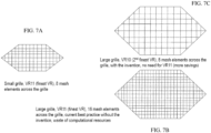
- FIG. 7A is a schematic representation of a grille (represented by the hexagonal outline and a mesh overlay).
- the illustrated grille is a small one, and the VR region of the associated mesh is VR11 (e.g., the finest VR region) which, as shown, results in 8 rows of cells from the top of the grille to the bottom of the grille.
- VR11 e.g., the finest VR region
- FIG. 7B is a schematic representation of a grille (represented by the hexagonal outline and a mesh overlay).
- the illustrated grille is a larger one, and the VR region of the associated mesh is VR11 (e.g., the finest VR region) which, as shown, results in 16 rows of cells from the top of the grille to the bottom of the grille.
- This application of the VR11 mesh results in a waste (i.e., an inefficient use) of computational resources.
- FIG. 7C is a schematic representation of a grille (represented by the hexagonal outline and a mesh overlay).
- the illustrated grille is a larger one (like the one in FIG. 7B ), and the VR region of the associated mesh is VR10 (e.g., the second finest mesh) - automatically selected and applied by the computer 1000 based on the processes set forth herein -- which, as shown, results in 8 rows of cells from the top of the grille to the bottom of the grille.
- This application of the VR10 mesh results in an efficient use of computational resources and high accuracy of any simulations.
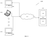
- FIG. 9 is a schematic representation of an implementation of a computer system 1100 configured to perform the functionalities disclosed herein.
- the illustrated computer system 1100 comprises a plurality of user workstations 1102a, 1102b ... 1102n and a server 1104 with computer memory 1106 and a computer processor 1108.
- the workstations 1102a, 1102b ... 1102n are coupled to the server 1104 and to each other via a communications network 1110 that enables communication therebetween.
- each of the user workstations 1102a, 1102b ...1102n may be implemented as a computer (e.g., computer 1000) with computer memory, storage, a computer processor, I/O device interface (with one or more connected I/O devices), and a network interface (connected to the network 1110 to facilitate communications with other network-connected devices).
- the server 1104 may be configured with storage, I/O device interface (with one or more connected I/O devices), and a network interface (connected to the network 1110 to facilitate communications with other network-connected devices).
- the computer system 1100 is configured to implement the systems and techniques disclosed herein. In doing so, however, various implementations of the system 1100 may distribute various memory and processing functionalities among multiple different system components across the system. In a typical implementation, human users can access and interact with the system 1100 from any one or more of the user workstations 1102a, 1102b ... 1102n and processing / memory functions may be performed at those user workstations and / or at processor 1104 with communications therebetween occurring via network 1110.
- systems and techniques disclosed herein are not limited to grilles on vehicles but could be extended to apply to virtually any kind of grille that facilitates and/or controls air or fluid flow.
- the systems and techniques disclosed herein can be integrated into automated simulation workflows to automatically create 3D digital geometries to define varied variable resolution (VR) meshing regions for simulating grilles.
- the systems and techniques can be utilized to quickly create multiple grille models with varied external shape designs in order to perform fast-turnaround simulations at the early design stage.
- the ray casting process is not limited to casting rays toward the image of the modeled object (e.g., car) from all directions. In some implementations, rays may be cast toward the modeled object from any two or more directions.
- the various methods and machines described herein may each be implemented by a physical, virtual, or hybrid general purpose computer, such as a computer system, or a computer network environment, such as those described herein.
- the computer / system may be transformed into the machines that execute the methods described herein, for example, by loading software instructions into either memory or non-volatile storage for execution by the CPU.
- the computer / system and its various components may be configured to carry out any embodiments or combination of embodiments of the present invention described herein.
- the system may implement the various embodiments described herein utilizing any combination of hardware, software, and firmware modules operatively coupled, internally, or externally, to or incorporated into the computer / system.
- the subject matter disclosed herein can be implemented in digital electronic circuitry, or in computer-based software, firmware, or hardware, including the structures disclosed in this specification and/or their structural equivalents, and/or in combinations thereof.
- the subject matter disclosed herein can be implemented in one or more computer programs, that is, one or more modules of computer program instructions, encoded on computer storage medium for execution by, or to control the operation of, one or more data processing apparatuses (e.g., processors).
- the program instructions can be encoded on an artificially generated propagated signal, for example, a machine-generated electrical, optical, or electromagnetic signal that is generated to encode information for transmission to suitable receiver apparatus for execution by a data processing apparatus.
- a computer storage medium can be, or can be included within, a computer-readable storage device, a computer-readable storage substrate, a random or serial access memory array or device, or a combination thereof. While a computer storage medium should not be considered to be solely a propagated signal, a computer storage medium may be a source or destination of computer program instructions encoded in an artificially generated propagated signal. The computer storage medium can also be, or be included in, one or more separate physical components or media, for example, multiple CDs, computer disks, and/or other storage devices.
- processor e.g., a processor / specially programmed processor / computer
- data processing apparatus e.g., a processor / specially programmed processor / computer
- processor encompasses all kinds of apparatus, devices, and machines for processing data, including by way of example a programmable processor, a computer, a system on a chip, or multiple ones, or combinations, of the foregoing.
- the apparatus can include special purpose logic circuitry, e.g., an FPGA (field programmable gate array) or an ASIC (application specific integrated circuit).
- the apparatus can also include, in addition to hardware, code that creates an execution environment for the computer program in question, for example, code that constitutes processor firmware, a protocol stack, a database management system, an operating system, a cross-platform runtime environment, a virtual machine, or a combination of one or more of them.
- the apparatus and execution environment can realize various different computing model infrastructures, such as web services, distributed computing, and grid computing infrastructures.
- Each functional component mentioned herein may be implemented, for example, by one of more computer hardware components (e.g., one or more computer processors) executing specially programmed computer readable instructions stored on computer-readable media (e.g., hardware memory in the form of RAM, ROM, etc.) to perform the associated computer-implemented functionalities described herein.
- computer hardware components e.g., one or more computer processors
- computer-readable media e.g., hardware memory in the form of RAM, ROM, etc.
- the systems and techniques disclosed herein may be utilized in connection with the overall design, analysis, and real-world manufacturing of an object (e.g., a grille).
- the simulation processes disclosed herein may be utilized to analyze the performance or behavior of the modeled object (e.g., grille) to confirm expectations or to guide further iterations in the design of the modeled object, and/or associated systems (that will include the grille).
- the design and analysis / simulation will be followed by manufacturing a real-world version of the modeled object (e.g., grille) based on a final design that has been exposed to computer-based simulations, prior to manufacturing, utilizing the systems and techniques disclosed herein.
- the final manufactured real world version of the modeled object would be a physical thing (e.g., a grille or the like).
Landscapes
- Engineering & Computer Science (AREA)
- Physics & Mathematics (AREA)
- Theoretical Computer Science (AREA)
- General Physics & Mathematics (AREA)
- Geometry (AREA)
- Computer Hardware Design (AREA)
- General Engineering & Computer Science (AREA)
- Evolutionary Computation (AREA)
- Mathematical Analysis (AREA)
- Mathematical Optimization (AREA)
- Pure & Applied Mathematics (AREA)
- Computer Vision & Pattern Recognition (AREA)
- Algebra (AREA)
- Mathematical Physics (AREA)
- Fluid Mechanics (AREA)
- Computing Systems (AREA)
- Computer Graphics (AREA)
- Multimedia (AREA)
- Computational Mathematics (AREA)
- Software Systems (AREA)
- Management, Administration, Business Operations System, And Electronic Commerce (AREA)
- Processing Or Creating Images (AREA)
- Image Analysis (AREA)
Applications Claiming Priority (1)
| Application Number | Priority Date | Filing Date | Title |
|---|---|---|---|
| US18/175,670 US20240289520A1 (en) | 2023-02-28 | 2023-02-28 | Automatic determination of ventilation grille opening size for numerical simulation setup automation |
Publications (1)
| Publication Number | Publication Date |
|---|---|
| EP4425367A1 true EP4425367A1 (de) | 2024-09-04 |
Family
ID=90105111
Family Applications (1)
| Application Number | Title | Priority Date | Filing Date |
|---|---|---|---|
| EP24160114.5A Pending EP4425367A1 (de) | 2023-02-28 | 2024-02-27 | Automatische bestimmung der lüftungsgitteröffnungsgrösse für die automation einer einrichtung zur numerischen simulation |
Country Status (4)
| Country | Link |
|---|---|
| US (1) | US20240289520A1 (de) |
| EP (1) | EP4425367A1 (de) |
| JP (1) | JP2024122909A (de) |
| CN (1) | CN118568912A (de) |
Families Citing this family (5)
| Publication number | Priority date | Publication date | Assignee | Title |
|---|---|---|---|---|
| USD1075587S1 (en) * | 2023-07-26 | 2025-05-20 | GM Global Technology Operations LLC | Vehicle upper grille |
| USD1080479S1 (en) * | 2023-07-31 | 2025-06-24 | GM Global Technology Operations LLC | Vehicle upper grille |
| USD1082623S1 (en) * | 2024-01-02 | 2025-07-08 | GM Global Technology Operations LLC | Vehicle upper grille |
| CN120145563B (zh) * | 2025-05-15 | 2025-07-25 | 中国空气动力研究与发展中心计算空气动力研究所 | 一种点与非规则六面体单元位置关系判定方法、装置、设备及存储介质 |
| CN120217611B (zh) * | 2025-05-28 | 2025-11-14 | 中家院(北京)检测认证有限公司 | 一种基于粒子群算法的翼型格栅设计方法及系统 |
Citations (1)
| Publication number | Priority date | Publication date | Assignee | Title |
|---|---|---|---|---|
| EP3809308A1 (de) * | 2019-10-17 | 2021-04-21 | Dassault Systemes Simulia Corp. | Verfahren zur automatischen berechnung der grösse der kreisförmigen öffnung einer axiallüfterhaube |
-
2023
- 2023-02-28 US US18/175,670 patent/US20240289520A1/en active Pending
-
2024
- 2024-02-26 JP JP2024026478A patent/JP2024122909A/ja active Pending
- 2024-02-27 EP EP24160114.5A patent/EP4425367A1/de active Pending
- 2024-02-28 CN CN202410223055.2A patent/CN118568912A/zh active Pending
Patent Citations (1)
| Publication number | Priority date | Publication date | Assignee | Title |
|---|---|---|---|---|
| EP3809308A1 (de) * | 2019-10-17 | 2021-04-21 | Dassault Systemes Simulia Corp. | Verfahren zur automatischen berechnung der grösse der kreisförmigen öffnung einer axiallüfterhaube |
Non-Patent Citations (6)
| Title |
|---|
| BRADSKI, G., THE OPENCV LIBRARY. DR. DOBB'S JOURNAL OF SOFTWARE TOOLS, 2000 |
| CANNY, J.: "A Computational Approach to Edge Detection", TRANSACTIONS ON PATTERN ANALYSIS AND MACHINE INTELLIGENCE, vol. 8, pages 679 - 698 |
| JOSEPH O'ROURKE: "International Journal of Computer & Information Sciences", FINDING MINIMAL ENCLOSING BOXES, 1985, pages 183 - 199 |
| KIM H J ET AL: "A numerical analysis for the cooling module related to automobile air-conditioning system", APPLIED THERMAL ENGINEERING, PERGAMON, OXFORD, GB, vol. 28, no. 14-15, 1 October 2008 (2008-10-01), pages 1896 - 1905, XP022850614, ISSN: 1359-4311, [retrieved on 20071214], DOI: 10.1016/J.APPLTHERMALENG.2007.12.002 * |
| SATOSHI SUZUK ET AL., TOPOLOGICAL STRUCTURAL ANALYSIS OF DIGITIZED BINARY IMAGES BY BORDER FOLLOWING, IN COMPUTER VISION, GRAPHICS, AND IMAGE PROCESSING, vol. 30, no. 1, 1985, pages 32 - 46 |
| SHAMOS, M., COMPUTATIONAL GEOMETRY, 1978, pages 76 - 81 |
Also Published As
| Publication number | Publication date |
|---|---|
| CN118568912A (zh) | 2024-08-30 |
| US20240289520A1 (en) | 2024-08-29 |
| JP2024122909A (ja) | 2024-09-09 |
Similar Documents
| Publication | Publication Date | Title |
|---|---|---|
| EP4425367A1 (de) | Automatische bestimmung der lüftungsgitteröffnungsgrösse für die automation einer einrichtung zur numerischen simulation | |
| US12307595B2 (en) | Automatic creation of three-dimensional (3D) variable resolution region geometries | |
| EP3258445B1 (de) | Okklusion für erweiterte realität | |
| EP3353750B1 (de) | Verfahren und systeme zur erkennung und kombination von strukturmerkmalen bei der 3d-rekonstruktion | |
| US11100710B2 (en) | Extracting a feature tree from a mesh | |
| CN102282561B (zh) | 冲突判定装置以及冲突判定方法 | |
| GB2456301A (en) | Surface Representation from a Point Cloud | |
| Monica et al. | Surfel-based next best view planning | |
| CN116921932B (zh) | 焊接轨迹识别方法、装置、设备及存储介质 | |
| CN113129348A (zh) | 一种基于单目视觉的道路场景中车辆目标的三维重建方法 | |
| Pound et al. | A patch-based approach to 3D plant shoot phenotyping | |
| CN112825200B (zh) | 处理真实对象上的形状属性的3d信号 | |
| Wiemann et al. | Automatic Map Creation For Environment Modelling In Robotic Simulators. | |
| CN110060346B (zh) | 确定代表真实对象皮肤的小面的集合 | |
| CN104573144A (zh) | 量测设备离线点云模拟系统及方法 | |
| Fischer et al. | Surveillance of robots using multiple colour or depth cameras with distributed processing | |
| Borodin et al. | Consistent normal orientation for polygonal meshes | |
| CN114022414A (zh) | 一种基于双目感知学习的加油加电智能动作的执行方法 | |
| Díaz-Vilariño et al. | From point clouds to 3D isovists in indoor environments | |
| CN116046017B (zh) | 一种测量路径的校准方法、装置、存储介质和计算机设备 | |
| Ososinski et al. | Multi-viewpoint visibility coverage estimation for 3D environment perception volumetric representation as a gateway to high resolution data | |
| CN117786867A (zh) | 圆角检测方法、系统、程序和存储介质 | |
| CN115393549A (zh) | 一种碰撞检测方法、系统及电子设备 | |
| Murray et al. | Environment modeling with stereo vision. | |
| Wright et al. | Algorithmic approach to planar void detection and validation in point clouds |
Legal Events
| Date | Code | Title | Description |
|---|---|---|---|
| PUAI | Public reference made under article 153(3) epc to a published international application that has entered the european phase |
Free format text: ORIGINAL CODE: 0009012 |
|
| STAA | Information on the status of an ep patent application or granted ep patent |
Free format text: STATUS: THE APPLICATION HAS BEEN PUBLISHED |
|
| AK | Designated contracting states |
Kind code of ref document: A1 Designated state(s): AL AT BE BG CH CY CZ DE DK EE ES FI FR GB GR HR HU IE IS IT LI LT LU LV MC ME MK MT NL NO PL PT RO RS SE SI SK SM TR |
|
| STAA | Information on the status of an ep patent application or granted ep patent |
Free format text: STATUS: REQUEST FOR EXAMINATION WAS MADE |
|
| 17P | Request for examination filed |
Effective date: 20250304 |