TW201802492A - Method and system for monitoring land deformation - Google Patents
Method and system for monitoring land deformation Download PDFInfo
- Publication number
- TW201802492A TW201802492A TW106113658A TW106113658A TW201802492A TW 201802492 A TW201802492 A TW 201802492A TW 106113658 A TW106113658 A TW 106113658A TW 106113658 A TW106113658 A TW 106113658A TW 201802492 A TW201802492 A TW 201802492A
- Authority
- TW
- Taiwan
- Prior art keywords
- receiver
- solution
- estimate
- relative orientation
- node
- Prior art date
Links
- 238000000034 method Methods 0.000 title claims description 117
- 238000012544 monitoring process Methods 0.000 title description 14
- 235000019892 Stellar Nutrition 0.000 claims description 97
- 239000011159 matrix material Substances 0.000 claims description 38
- 238000007667 floating Methods 0.000 claims description 37
- 238000012935 Averaging Methods 0.000 claims description 10
- 238000004422 calculation algorithm Methods 0.000 description 136
- 238000001914 filtration Methods 0.000 description 71
- 230000033001 locomotion Effects 0.000 description 62
- 238000005259 measurement Methods 0.000 description 62
- 230000008859 change Effects 0.000 description 51
- 238000012360 testing method Methods 0.000 description 46
- 239000003990 capacitor Substances 0.000 description 32
- 230000002354 daily effect Effects 0.000 description 30
- 230000006872 improvement Effects 0.000 description 30
- 238000009826 distribution Methods 0.000 description 28
- 230000000694 effects Effects 0.000 description 26
- 230000003068 static effect Effects 0.000 description 25
- 230000005540 biological transmission Effects 0.000 description 24
- 230000006870 function Effects 0.000 description 24
- 238000004088 simulation Methods 0.000 description 23
- 239000013598 vector Substances 0.000 description 22
- 238000012937 correction Methods 0.000 description 16
- 238000004364 calculation method Methods 0.000 description 15
- 238000004806 packaging method and process Methods 0.000 description 15
- 230000009467 reduction Effects 0.000 description 14
- 230000008901 benefit Effects 0.000 description 10
- 238000006073 displacement reaction Methods 0.000 description 10
- 239000000463 material Substances 0.000 description 10
- 230000004044 response Effects 0.000 description 10
- 125000004122 cyclic group Chemical group 0.000 description 9
- 238000007726 management method Methods 0.000 description 9
- NMOBGFHEUQQCPQ-PCLQRYFVSA-N [2-(carbamoyloxymethyl)-2-methylpentyl] carbamate;[(9s,13s,14s)-13-methyl-17-oxo-9,11,12,14,15,16-hexahydro-6h-cyclopenta[a]phenanthren-3-yl] hydrogen sulfate;[(8r,9s,13s,14s)-13-methyl-17-oxo-7,8,9,11,12,14,15,16-octahydro-6h-cyclopenta[a]phenanthren-3-y Chemical compound NC(=O)OCC(C)(CCC)COC(N)=O.OS(=O)(=O)OC1=CC=C2[C@H]3CC[C@](C)(C(CC4)=O)[C@@H]4[C@@H]3CCC2=C1.OS(=O)(=O)OC1=CC=C2[C@H]3CC[C@](C)(C(CC4)=O)[C@@H]4C3=CCC2=C1.OS(=O)(=O)OC1=CC=C2C(CC[C@]3([C@H]4CCC3=O)C)=C4C=CC2=C1 NMOBGFHEUQQCPQ-PCLQRYFVSA-N 0.000 description 8
- 238000012545 processing Methods 0.000 description 8
- 230000002829 reductive effect Effects 0.000 description 8
- 235000004522 Pentaglottis sempervirens Nutrition 0.000 description 7
- 239000002131 composite material Substances 0.000 description 7
- 238000013461 design Methods 0.000 description 7
- 238000010586 diagram Methods 0.000 description 7
- 230000008569 process Effects 0.000 description 7
- XLYOFNOQVPJJNP-UHFFFAOYSA-N water Substances O XLYOFNOQVPJJNP-UHFFFAOYSA-N 0.000 description 7
- 230000000903 blocking effect Effects 0.000 description 6
- 230000027288 circadian rhythm Effects 0.000 description 6
- 238000004891 communication Methods 0.000 description 6
- 230000003203 everyday effect Effects 0.000 description 6
- 230000007774 longterm Effects 0.000 description 6
- 230000001360 synchronised effect Effects 0.000 description 6
- UOAFGUOASVSLPK-UHFFFAOYSA-N 1-(2-chloroethyl)-3-(2,2-dimethylpropyl)-1-nitrosourea Chemical compound CC(C)(C)CNC(=O)N(N=O)CCCl UOAFGUOASVSLPK-UHFFFAOYSA-N 0.000 description 5
- 230000001419 dependent effect Effects 0.000 description 5
- 238000002474 experimental method Methods 0.000 description 5
- 230000009897 systematic effect Effects 0.000 description 5
- 230000001960 triggered effect Effects 0.000 description 5
- 239000002699 waste material Substances 0.000 description 5
- 241000257303 Hymenoptera Species 0.000 description 4
- 241000233805 Phoenix Species 0.000 description 4
- 239000000654 additive Substances 0.000 description 4
- 230000000996 additive effect Effects 0.000 description 4
- 238000010276 construction Methods 0.000 description 4
- 230000002596 correlated effect Effects 0.000 description 4
- 230000004069 differentiation Effects 0.000 description 4
- 238000013213 extrapolation Methods 0.000 description 4
- NIHNNTQXNPWCJQ-UHFFFAOYSA-N fluorene Chemical compound C1=CC=C2CC3=CC=CC=C3C2=C1 NIHNNTQXNPWCJQ-UHFFFAOYSA-N 0.000 description 4
- 239000005433 ionosphere Substances 0.000 description 4
- 230000000737 periodic effect Effects 0.000 description 4
- 230000002093 peripheral effect Effects 0.000 description 4
- 238000005070 sampling Methods 0.000 description 4
- 230000001133 acceleration Effects 0.000 description 3
- 230000009471 action Effects 0.000 description 3
- 238000004458 analytical method Methods 0.000 description 3
- 238000000354 decomposition reaction Methods 0.000 description 3
- 238000005265 energy consumption Methods 0.000 description 3
- 230000000670 limiting effect Effects 0.000 description 3
- 229910052751 metal Inorganic materials 0.000 description 3
- 239000002184 metal Substances 0.000 description 3
- 239000000047 product Substances 0.000 description 3
- 238000009987 spinning Methods 0.000 description 3
- 230000002123 temporal effect Effects 0.000 description 3
- 230000007704 transition Effects 0.000 description 3
- 244000025254 Cannabis sativa Species 0.000 description 2
- 230000015572 biosynthetic process Effects 0.000 description 2
- 239000011248 coating agent Substances 0.000 description 2
- 238000000576 coating method Methods 0.000 description 2
- 238000013016 damping Methods 0.000 description 2
- 238000001514 detection method Methods 0.000 description 2
- 230000009977 dual effect Effects 0.000 description 2
- 238000011156 evaluation Methods 0.000 description 2
- 238000011049 filling Methods 0.000 description 2
- 238000003384 imaging method Methods 0.000 description 2
- 230000008676 import Effects 0.000 description 2
- 238000013101 initial test Methods 0.000 description 2
- 238000009434 installation Methods 0.000 description 2
- 230000010354 integration Effects 0.000 description 2
- 230000000116 mitigating effect Effects 0.000 description 2
- 238000002156 mixing Methods 0.000 description 2
- 230000036961 partial effect Effects 0.000 description 2
- JTJMJGYZQZDUJJ-UHFFFAOYSA-N phencyclidine Chemical class C1CCCCN1C1(C=2C=CC=CC=2)CCCCC1 JTJMJGYZQZDUJJ-UHFFFAOYSA-N 0.000 description 2
- 238000011160 research Methods 0.000 description 2
- 238000000926 separation method Methods 0.000 description 2
- 230000007958 sleep Effects 0.000 description 2
- FXWALQSAZZPDOT-NMUGVGKYSA-N Arg-Thr-Cys-Cys Chemical compound SC[C@@H](C(O)=O)NC(=O)[C@H](CS)NC(=O)[C@H]([C@H](O)C)NC(=O)[C@@H](N)CCCNC(N)=N FXWALQSAZZPDOT-NMUGVGKYSA-N 0.000 description 1
- 241000196324 Embryophyta Species 0.000 description 1
- 239000004593 Epoxy Substances 0.000 description 1
- 101100172132 Mus musculus Eif3a gene Proteins 0.000 description 1
- 208000012868 Overgrowth Diseases 0.000 description 1
- 230000002159 abnormal effect Effects 0.000 description 1
- 230000005856 abnormality Effects 0.000 description 1
- 238000009825 accumulation Methods 0.000 description 1
- 230000002411 adverse Effects 0.000 description 1
- 230000032683 aging Effects 0.000 description 1
- RJGDLRCDCYRQOQ-UHFFFAOYSA-N anthrone Chemical compound C1=CC=C2C(=O)C3=CC=CC=C3CC2=C1 RJGDLRCDCYRQOQ-UHFFFAOYSA-N 0.000 description 1
- 238000013459 approach Methods 0.000 description 1
- 230000001174 ascending effect Effects 0.000 description 1
- 239000010426 asphalt Substances 0.000 description 1
- 230000009286 beneficial effect Effects 0.000 description 1
- 239000000969 carrier Substances 0.000 description 1
- 230000001413 cellular effect Effects 0.000 description 1
- 230000002060 circadian Effects 0.000 description 1
- 230000006835 compression Effects 0.000 description 1
- 238000007906 compression Methods 0.000 description 1
- 238000007796 conventional method Methods 0.000 description 1
- 230000000875 corresponding effect Effects 0.000 description 1
- 230000007797 corrosion Effects 0.000 description 1
- 238000005260 corrosion Methods 0.000 description 1
- 230000009193 crawling Effects 0.000 description 1
- 239000013078 crystal Substances 0.000 description 1
- 238000013480 data collection Methods 0.000 description 1
- 238000013075 data extraction Methods 0.000 description 1
- 230000007423 decrease Effects 0.000 description 1
- 238000009795 derivation Methods 0.000 description 1
- 230000008030 elimination Effects 0.000 description 1
- 238000003379 elimination reaction Methods 0.000 description 1
- 238000004146 energy storage Methods 0.000 description 1
- 238000005516 engineering process Methods 0.000 description 1
- 230000007613 environmental effect Effects 0.000 description 1
- 239000003822 epoxy resin Substances 0.000 description 1
- 230000003631 expected effect Effects 0.000 description 1
- 238000009499 grossing Methods 0.000 description 1
- 230000009474 immediate action Effects 0.000 description 1
- 238000011423 initialization method Methods 0.000 description 1
- 238000007689 inspection Methods 0.000 description 1
- 239000002932 luster Substances 0.000 description 1
- 238000013507 mapping Methods 0.000 description 1
- 230000007246 mechanism Effects 0.000 description 1
- 238000012986 modification Methods 0.000 description 1
- 230000004048 modification Effects 0.000 description 1
- 230000008450 motivation Effects 0.000 description 1
- 230000003287 optical effect Effects 0.000 description 1
- 238000012856 packing Methods 0.000 description 1
- 239000002245 particle Substances 0.000 description 1
- 238000011056 performance test Methods 0.000 description 1
- 238000000819 phase cycle Methods 0.000 description 1
- 230000010363 phase shift Effects 0.000 description 1
- 229920000647 polyepoxide Polymers 0.000 description 1
- 230000003334 potential effect Effects 0.000 description 1
- 239000002994 raw material Substances 0.000 description 1
- 230000008707 rearrangement Effects 0.000 description 1
- 230000008929 regeneration Effects 0.000 description 1
- 238000011069 regeneration method Methods 0.000 description 1
- 230000001105 regulatory effect Effects 0.000 description 1
- 230000003252 repetitive effect Effects 0.000 description 1
- 230000000717 retained effect Effects 0.000 description 1
- 230000002441 reversible effect Effects 0.000 description 1
- 230000001932 seasonal effect Effects 0.000 description 1
- 230000001568 sexual effect Effects 0.000 description 1
- 230000035939 shock Effects 0.000 description 1
- 230000011664 signaling Effects 0.000 description 1
- 229910052709 silver Inorganic materials 0.000 description 1
- 239000004332 silver Substances 0.000 description 1
- 239000002689 soil Substances 0.000 description 1
- 239000007787 solid Substances 0.000 description 1
- 238000010561 standard procedure Methods 0.000 description 1
- 239000013589 supplement Substances 0.000 description 1
- 239000000725 suspension Substances 0.000 description 1
- 230000008961 swelling Effects 0.000 description 1
- 230000001052 transient effect Effects 0.000 description 1
- 238000009827 uniform distribution Methods 0.000 description 1
- 238000012795 verification Methods 0.000 description 1
Classifications
-
- G—PHYSICS
- G01—MEASURING; TESTING
- G01S—RADIO DIRECTION-FINDING; RADIO NAVIGATION; DETERMINING DISTANCE OR VELOCITY BY USE OF RADIO WAVES; LOCATING OR PRESENCE-DETECTING BY USE OF THE REFLECTION OR RERADIATION OF RADIO WAVES; ANALOGOUS ARRANGEMENTS USING OTHER WAVES
- G01S19/00—Satellite radio beacon positioning systems; Determining position, velocity or attitude using signals transmitted by such systems
- G01S19/38—Determining a navigation solution using signals transmitted by a satellite radio beacon positioning system
- G01S19/39—Determining a navigation solution using signals transmitted by a satellite radio beacon positioning system the satellite radio beacon positioning system transmitting time-stamped messages, e.g. GPS [Global Positioning System], GLONASS [Global Orbiting Navigation Satellite System] or GALILEO
- G01S19/42—Determining position
- G01S19/43—Determining position using carrier phase measurements, e.g. kinematic positioning; using long or short baseline interferometry
- G01S19/44—Carrier phase ambiguity resolution; Floating ambiguity; LAMBDA [Least-squares AMBiguity Decorrelation Adjustment] method
-
- G—PHYSICS
- G01—MEASURING; TESTING
- G01S—RADIO DIRECTION-FINDING; RADIO NAVIGATION; DETERMINING DISTANCE OR VELOCITY BY USE OF RADIO WAVES; LOCATING OR PRESENCE-DETECTING BY USE OF THE REFLECTION OR RERADIATION OF RADIO WAVES; ANALOGOUS ARRANGEMENTS USING OTHER WAVES
- G01S19/00—Satellite radio beacon positioning systems; Determining position, velocity or attitude using signals transmitted by such systems
- G01S19/01—Satellite radio beacon positioning systems transmitting time-stamped messages, e.g. GPS [Global Positioning System], GLONASS [Global Orbiting Navigation Satellite System] or GALILEO
- G01S19/13—Receivers
- G01S19/24—Acquisition or tracking or demodulation of signals transmitted by the system
- G01S19/28—Satellite selection
-
- G—PHYSICS
- G01—MEASURING; TESTING
- G01S—RADIO DIRECTION-FINDING; RADIO NAVIGATION; DETERMINING DISTANCE OR VELOCITY BY USE OF RADIO WAVES; LOCATING OR PRESENCE-DETECTING BY USE OF THE REFLECTION OR RERADIATION OF RADIO WAVES; ANALOGOUS ARRANGEMENTS USING OTHER WAVES
- G01S19/00—Satellite radio beacon positioning systems; Determining position, velocity or attitude using signals transmitted by such systems
- G01S19/38—Determining a navigation solution using signals transmitted by a satellite radio beacon positioning system
- G01S19/39—Determining a navigation solution using signals transmitted by a satellite radio beacon positioning system the satellite radio beacon positioning system transmitting time-stamped messages, e.g. GPS [Global Positioning System], GLONASS [Global Orbiting Navigation Satellite System] or GALILEO
- G01S19/42—Determining position
- G01S19/51—Relative positioning
-
- G—PHYSICS
- G08—SIGNALLING
- G08C—TRANSMISSION SYSTEMS FOR MEASURED VALUES, CONTROL OR SIMILAR SIGNALS
- G08C17/00—Arrangements for transmitting signals characterised by the use of a wireless electrical link
- G08C17/02—Arrangements for transmitting signals characterised by the use of a wireless electrical link using a radio link
-
- G—PHYSICS
- G01—MEASURING; TESTING
- G01S—RADIO DIRECTION-FINDING; RADIO NAVIGATION; DETERMINING DISTANCE OR VELOCITY BY USE OF RADIO WAVES; LOCATING OR PRESENCE-DETECTING BY USE OF THE REFLECTION OR RERADIATION OF RADIO WAVES; ANALOGOUS ARRANGEMENTS USING OTHER WAVES
- G01S19/00—Satellite radio beacon positioning systems; Determining position, velocity or attitude using signals transmitted by such systems
- G01S19/01—Satellite radio beacon positioning systems transmitting time-stamped messages, e.g. GPS [Global Positioning System], GLONASS [Global Orbiting Navigation Satellite System] or GALILEO
- G01S19/13—Receivers
- G01S19/34—Power consumption
-
- G—PHYSICS
- G01—MEASURING; TESTING
- G01S—RADIO DIRECTION-FINDING; RADIO NAVIGATION; DETERMINING DISTANCE OR VELOCITY BY USE OF RADIO WAVES; LOCATING OR PRESENCE-DETECTING BY USE OF THE REFLECTION OR RERADIATION OF RADIO WAVES; ANALOGOUS ARRANGEMENTS USING OTHER WAVES
- G01S19/00—Satellite radio beacon positioning systems; Determining position, velocity or attitude using signals transmitted by such systems
- G01S19/38—Determining a navigation solution using signals transmitted by a satellite radio beacon positioning system
- G01S19/39—Determining a navigation solution using signals transmitted by a satellite radio beacon positioning system the satellite radio beacon positioning system transmitting time-stamped messages, e.g. GPS [Global Positioning System], GLONASS [Global Orbiting Navigation Satellite System] or GALILEO
- G01S19/42—Determining position
Landscapes
- Engineering & Computer Science (AREA)
- Radar, Positioning & Navigation (AREA)
- Remote Sensing (AREA)
- Computer Networks & Wireless Communication (AREA)
- Physics & Mathematics (AREA)
- General Physics & Mathematics (AREA)
- Position Fixing By Use Of Radio Waves (AREA)
Abstract
Description
發明領域 Field of invention
本發明係關於一種用於監測地面變形,特別是用於監測地滑移動型樣(landslide movement pattern)的方法及系統。 The present invention relates to a method and system for monitoring ground deformation, particularly for monitoring a landslide movement pattern.
發明背景 Background of the invention
儘管近來可用諸如基於雷射之測地技術、基於GPS之系統及基於地面/衛星之雷達的技術,但地滑移動型樣之監測仍然是一種挑戰。 Despite the recent availability of technologies such as laser-based geodetic techniques, GPS-based systems, and terrestrial/satellite-based radars, the monitoring of ground-slip mobile patterns remains a challenge.
使用中的大多數(若非全部)現有技術依賴於地滑區中稀疏部署之監測點之準確位置資訊的可用性,以及來自其他感測裝置之資料。使用中的各種類型之感測器(包括伸長計、固定式測斜計、傾斜計、壓力換能器及雨量計)全部往往會昂貴。此高成本往往會將其部署僅限制至風險非常高的位點。 Most, if not all, of the prior art in use relies on the availability of accurate location information for sparsely deployed monitoring points in the land slide zone, as well as data from other sensing devices. The various types of sensors in use (including extensometers, fixed inclinometers, inclinometers, pressure transducers, and rain gauges) are often expensive. This high cost tends to limit its deployment to only very high risk sites.
先前系統之另外缺點為其需要持續的電源。實務上,並不總是能得到持續的電源,此意謂不能連續地得到GPS資料。此又潛在不利地影響典型的基於GPS 之定位系統的準確度。 Another disadvantage of previous systems was that they required a continuous power supply. In practice, it is not always possible to get a continuous power supply, which means that GPS data cannot be obtained continuously. This potentially adversely affects typical GPS-based The accuracy of the positioning system.
本發明之至少較佳實施例的一目標係處理前述缺點中之一些。額外或替代目標係至少將有用的選擇提供給公眾。 One object of at least one preferred embodiment of the present invention is to address some of the aforementioned disadvantages. Additional or alternative goals are at least useful to the public.
發明概要 Summary of invention
根據本發明之一態樣,一種判定相關聯於一第一接收器及一第二接收器之一相對方位的方法包含:接收相關聯於一第一接收器之第一位置資料;接收相關聯於一第二接收器之第二位置資料;判定相關聯於該第一接收器及該第二接收器之一第一估計相對方位;至少部分地自該第一估計相對方位判定相關聯於該第一接收器及該第二接收器之一第二估計相對方位;至少部分地自該第二估計相對方位判定相關聯於該第一接收器及該第二接收器之一第三估計相對方位;及至少部分地自該第三估計相對方位判定相關聯於該第一接收器及該第二接收器之一第四估計相對方位。 According to one aspect of the invention, a method of determining a relative orientation associated with a first receiver and a second receiver includes: receiving a first location profile associated with a first receiver; receiving an association a second location data of a second receiver; determining a first estimated relative orientation associated with one of the first receiver and the second receiver; at least partially associated with the first estimated relative orientation determination a second estimated relative orientation of the first receiver and the second receiver; at least in part from the second estimated relative orientation determination associated with a third estimated relative orientation of the first receiver and the second receiver And determining, at least in part from the third estimated relative orientation, a fourth estimated relative orientation associated with one of the first receiver and the second receiver.
如本說明書中所使用之術語「包含(comprising)」意謂「至少部分地由……組成」。當解譯本說明書中包括術語「包含」之每一語句時,亦可存在除了前面有該術語之彼或彼等特徵以外的特徵。應以相同方式解譯諸如「包含(comprise)」及「包含(comprises)」之相關術語。 The term "comprising" as used in this specification means "consisting at least in part of". When interpreting each statement in the specification including the term "comprising", there may also be a feature other than the one or the one of the above. Terms such as "comprise" and "comprises" should be interpreted in the same way.
在一實施例中,判定該第一相對方位包含: 判定相關聯於該第一接收器之一第一自主方位與相關聯於該第二接收器之一第二自主方位之間的一差。 In an embodiment, determining the first relative orientation comprises: A difference between a first autonomous orientation associated with one of the first receivers and a second autonomous orientation associated with one of the second receivers is determined.
在一實施例中,該第一位置資料及/或該第二位置資料包含一共同秒基曆元、一衛星識別符、一接收器識別符、一時間、一平均化自主方位中之一或多者。 In an embodiment, the first location data and/or the second location profile includes one of a common second base epoch, a satellite identifier, a receiver identifier, a time, an averaged autonomous orientation, or More.
在一實施例中,判定該第二估計相對方位包含:接收相關聯於至少兩對衛星之各別雙差估計;形成相關聯於該等雙差估計之一觀測矩陣;及至少部分地自該觀測矩陣界定一解估計。 In an embodiment, determining the second estimated relative orientation comprises: receiving respective double-difference estimates associated with at least two pairs of satellites; forming an observation matrix associated with the two-difference estimates; and at least partially The observation matrix defines a solution estimate.
在一實施例中,判定該第三估計相對方位包含:接收至少一個模糊度估計;將該至少一個模糊度估計固定至各別整數模糊度估計;及至少部分地自該(等)整數模糊度估計界定一解。 In an embodiment, determining the third estimated relative orientation comprises: receiving at least one ambiguity estimate; fixing the at least one ambiguity estimate to a respective integer ambiguity estimate; and at least partially from the (equal) integer ambiguity Estimate a definition.
根據本發明之一另外態樣,一種判定相關聯於一第一接收器及一第二接收器之一相對方位的方法包含:接收相關聯於至少兩對衛星之各別雙差估計;形成相關聯於該等雙差估計之一觀測矩陣;及至少部分地自該觀測矩陣界定一解估計。 In accordance with still another aspect of the present invention, a method of determining a relative orientation associated with a first receiver and a second receiver includes: receiving respective double difference estimates associated with at least two pairs of satellites; Associated with one of the two different estimates of the observation matrix; and at least partially defines a solution estimate from the observation matrix.
在一實施例中,該方法進一步包含界定至少一個模糊度估計。 In an embodiment, the method further includes defining at least one ambiguity estimate.
在一實施例中,該方法進一步包含界定一共變數矩陣。 In an embodiment, the method further includes defining a common variable matrix.
根據本發明之一另外態樣,一種判定相關聯於一第一接收器及一第二接收器之一相對方位的方法包 含:接收至少一個模糊度估計;將該至少一個模糊度估計固定至各別整數模糊度估計;及至少部分地自該(等)整數模糊度估計界定一解。 According to another aspect of the present invention, a method package for determining a relative orientation associated with a first receiver and a second receiver Included: receiving at least one ambiguity estimate; fixing the at least one ambiguity estimate to a respective integer ambiguity estimate; and defining a solution at least in part from the (equal) integer ambiguity estimate.
在一實施例中,界定該解包含:獲得一第一解估計;捨位該第一解估計;及至少部分地自該經捨位之第一解估計獲得一第二解估計。 In an embodiment, defining the solution comprises: obtaining a first solution estimate; truncating the first solution estimate; and obtaining a second solution estimate at least in part from the first solution estimate of the truncated bit.
根據本發明之一另外態樣,一種用於判定相關聯於一第一接收器及一第二接收器之一相對方位的系統包含:一代碼模組,其經組配以接收相關聯於該第一接收器之位置資料,接收相關聯於該第二接收器之位置資料,且判定相關聯於該第一接收器及該第二接收器之一第一估計相對方位;一浮動模組,其經組配以至少部分地自該第一估計相對方位判定相關聯於該第一接收器及該第二接收器之一第二估計相對方位;一固定模組,其經組配以至少部分地自該第二估計相對方位判定相關聯於該第一接收器及該第二接收器之一第三估計相對方位;及一恆星模組,其經組配以至少部分地自該第三估計相對方位判定相關聯於該第一接收器及該第二接收器之一第四估計相對方位。 According to another aspect of the present invention, a system for determining a relative orientation associated with a first receiver and a second receiver includes: a code module configured to receive associated with the Position data of the first receiver, receiving location data associated with the second receiver, and determining a first estimated relative orientation associated with one of the first receiver and the second receiver; a floating module, Composing to determine, at least in part from the first estimated relative orientation, a second estimated relative orientation associated with one of the first receiver and the second receiver; a fixed module that is assembled to at least partially Determining, from the second estimated relative position, a third estimated relative orientation associated with one of the first receiver and the second receiver; and a star module configured to at least partially derive from the third estimate The relative orientation determination is associated with a fourth estimated relative orientation of one of the first receiver and the second receiver.
在一實施例中,該代碼模組經組配以藉由判定相關聯於該第一接收器之一第一自主方位與相關聯於該第二接收器之一第二自主方位之間的一差來判定該第一相對方位。 In one embodiment, the code module is configured to determine between a first autonomous orientation associated with one of the first receivers and a second autonomous orientation associated with one of the second receivers The difference is used to determine the first relative orientation.
在一實施例中,該第一位置資料及/或該第二位置資料包含一共同秒基曆元、一衛星識別符、一接收器 識別符、一時間、一平均化自主方位中之一或多者。 In an embodiment, the first location data and/or the second location profile includes a common second base epoch, a satellite identifier, and a receiver. One or more of an identifier, a time, and an average autonomous orientation.
在一實施例中,該浮動模組經組配以:接收相關聯於至少兩對衛星之各別雙差估計;形成相關聯於該等雙差估計之一觀測矩陣;及至少部分地自該觀測矩陣界定一解估計。 In one embodiment, the floating module is configured to: receive respective two-difference estimates associated with at least two pairs of satellites; form an observation matrix associated with the two-difference estimates; and at least partially from the The observation matrix defines a solution estimate.
在一實施例中,該固定模組經組配以:接收至少一個模糊度估計;將該至少一個模糊度估計固定至各別整數模糊度估計;及至少部分地自該(等)整數模糊度估計界定一解。 In an embodiment, the fixed module is configured to: receive at least one ambiguity estimate; fix the at least one ambiguity estimate to a respective integer ambiguity estimate; and at least partially from the (equal) integer ambiguity Estimate a definition.
根據本發明之一另外態樣,一種用於判定相關聯於一第一接收器及一第二接收器之一相對方位的系統包含一浮動模組,該浮動模組經組配以:接收相關聯於至少兩對衛星之各別雙差估計;形成相關聯於該等雙差估計之一觀測矩陣;及至少部分地自該觀測矩陣界定一解估計。 According to another aspect of the present invention, a system for determining a relative orientation associated with a first receiver and a second receiver includes a floating module that is configured to: receive correlation Associated with a respective two-difference estimate of at least two pairs of satellites; forming an observation matrix associated with one of the two-difference estimates; and at least partially defining a solution estimate from the observation matrix.
在一實施例中,該浮動模組經進一步組配以界定至少一個模糊度估計。 In an embodiment, the floating module is further configured to define at least one ambiguity estimate.
在一實施例中,該浮動模組經進一步組配以界定一共變數矩陣。 In an embodiment, the floating modules are further configured to define a common variable matrix.
根據本發明之一另外態樣,一種用於判定相關聯於一第一接收器及一第二接收器之一相對方位的系統包含一固定模組,該固定模組經組配以:接收至少一個模糊度估計;將該至少一個模糊度估計固定至各別整數模糊度估計;及至少部分地自該(等)整數模糊度估計界定一解。 According to another aspect of the present invention, a system for determining a relative orientation associated with a first receiver and a second receiver includes a fixed module, the fixed module being configured to: receive at least a ambiguity estimate; fixing the at least one ambiguity estimate to a respective integer ambiguity estimate; and at least partially defining a solution from the (equal) integer ambiguity estimate.
在一實施例中,該固定模組經進一步組配 以:藉由獲得一第一解估計來界定該解;捨位該第一解估計;及至少部分地自該經捨位之第一解估計獲得一第二解估計。 In an embodiment, the fixing module is further assembled And: defining the solution by obtaining a first solution estimate; truncating the first solution estimate; and obtaining a second solution estimate at least in part from the first solution estimate of the truncated bit.
根據本發明之一態樣,一種電腦可讀媒體在其上儲存有電腦可執行指令,該等電腦可執行指令在一計算裝置上被執行時致使該計算裝置進行一判定相關聯於一第一接收器及一第二接收器之一相對方位的方法,該方法包含:接收相關聯於一第一接收器之第一位置資料;接收相關聯於一第二接收器之第二位置資料;判定相關聯於該第一接收器及該第二接收器之一第一估計相對方位;至少部分地自該第一估計相對方位判定相關聯於該第一接收器及該第二接收器之一第二估計相對方位;至少部分地自該第二估計相對方位判定相關聯於該第一接收器及該第二接收器之一第三估計相對方位;及至少部分地自該第三估計相對方位判定相關聯於該第一接收器及該第二接收器之一第四估計相對方位。 According to one aspect of the invention, a computer readable medium having stored thereon computer executable instructions that, when executed on a computing device, cause the computing device to make a determination associated with a first A method for relative orientation of a receiver and a second receiver, the method comprising: receiving first location data associated with a first receiver; receiving second location data associated with a second receiver; determining Correlating a first estimated relative orientation of one of the first receiver and the second receiver; at least partially determining from the first estimated relative orientation that is associated with the first receiver and the second receiver Estimating a relative orientation; determining, at least in part from the second estimated relative orientation, a third estimated relative orientation associated with the first receiver and the second receiver; and determining, at least in part, from the third estimated relative orientation A fourth estimated relative orientation associated with one of the first receiver and the second receiver.
在一實施例中,判定該第一相對方位包含:判定相關聯於該第一接收器之一第一自主方位與相關聯於該第二接收器之一第二自主方位之間的一差。 In an embodiment, determining the first relative orientation comprises determining a difference between a first autonomous orientation associated with one of the first receivers and a second autonomous orientation associated with one of the second receivers.
在一實施例中,該第一位置資料及/或該第二位置資料包含一共同秒基曆元、一衛星識別符、一接收器識別符、一時間、一平均化自主方位中之一或多者。 In an embodiment, the first location data and/or the second location profile includes one of a common second base epoch, a satellite identifier, a receiver identifier, a time, an averaged autonomous orientation, or More.
在一實施例中,判定該第二估計相對方位包含:接收相關聯於至少兩對衛星之各別雙差估計;形成相 關聯於該等雙差估計之一觀測矩陣;及至少部分地自該觀測矩陣界定一解估計。 In an embodiment, determining the second estimated relative orientation comprises: receiving respective double difference estimates associated with at least two pairs of satellites; forming a phase Associated with one of the observation frames of the two-difference estimates; and at least partially defines a solution estimate from the observation matrix.
在一實施例中,判定該第三估計相對方位包含:接收至少一個模糊度估計;將該至少一個模糊度估計固定至各別整數模糊度估計;及至少部分地自該(等)整數模糊度估計界定一解。 In an embodiment, determining the third estimated relative orientation comprises: receiving at least one ambiguity estimate; fixing the at least one ambiguity estimate to a respective integer ambiguity estimate; and at least partially from the (equal) integer ambiguity Estimate a definition.
根據本發明之一另外態樣,一種電腦可讀媒體在其上儲存有電腦可執行指令,該等電腦可執行指令在一計算裝置上被執行時致使該計算裝置進行一判定相關聯於一第一接收器及一第二接收器之一相對方位的方法,該方法包含:接收相關聯於至少兩對衛星之各別雙差估計;形成相關聯於該等雙差估計之一觀測矩陣;及至少部分地自該觀測矩陣界定一解估計。 According to another aspect of the present invention, a computer readable medium having stored thereon computer executable instructions that, when executed on a computing device, cause the computing device to make a determination associated with a A method for relative orientation of a receiver and a second receiver, the method comprising: receiving respective double-difference estimates associated with at least two pairs of satellites; forming an observation matrix associated with the two-difference estimates; A solution estimate is defined at least in part from the observation matrix.
在一實施例中,該方法進一步包含界定至少一個模糊度估計。 In an embodiment, the method further includes defining at least one ambiguity estimate.
在一實施例中,該方法進一步包含界定一共變數矩陣。 In an embodiment, the method further includes defining a common variable matrix.
根據本發明之一另外態樣,一種電腦可讀媒體在其上儲存有電腦可執行指令,該等電腦可執行指令在一計算裝置上被執行時致使該計算裝置進行一判定相關聯於一第一接收器及一第二接收器之一相對方位的方法,該方法包含:接收至少一個模糊度估計;將該至少一個模糊度估計固定至各別整數模糊度估計;及至少部分地自該(等)整數模糊度估計界定一解。 According to another aspect of the present invention, a computer readable medium having stored thereon computer executable instructions that, when executed on a computing device, cause the computing device to make a determination associated with a A method for relative orientation of a receiver and a second receiver, the method comprising: receiving at least one ambiguity estimate; fixing the at least one ambiguity estimate to a respective integer ambiguity estimate; and at least partially from the Etc.) Integer ambiguity estimation defines a solution.
在一實施例中,界定該解包含:獲得一第一解估計;捨位該第一解估計;及至少部分地自該經捨位之第一解估計獲得一第二解估計。 In an embodiment, defining the solution comprises: obtaining a first solution estimate; truncating the first solution estimate; and obtaining a second solution estimate at least in part from the first solution estimate of the truncated bit.
在一個態樣中,本發明包含若干步驟。此等步驟中之一或多者相對於其他步驟中之每一者的關係、體現建構特徵之設備以及經調適以影響此等步驟之元件組合及部件配置全部在以下詳細揭示內容中被例示。 In one aspect, the invention encompasses several steps. The relationship of one or more of these steps with respect to each of the other steps, the device embodying the construction features, and the component combinations and component configurations adapted to affect such steps are all exemplified in the following detailed disclosure.
對於熟習本發明相關技術者而言,其自身將在不脫離如所附申請專利範圍中所界定的本發明之範疇的情況下想到許多建構改變以及本發明之廣泛不同的實施例及應用。本文中之揭示內容及描述純粹係說明性的,且並不意欲在任何意義上係限制性的。在本文中提及在本發明相關技術中具有已知等效者之特定整體的情況下,此等已知等效者被視為好像被個別地闡述而併入本文中。 Numerous construction changes and widely different embodiments and applications of the present invention will be apparent to those skilled in the art of the present invention without departing from the scope of the invention as defined in the appended claims. The disclosure and the description herein are purely illustrative and are not intended to be limiting in any sense. Where a specific whole of a known equivalent is found in the related art of the present invention, such known equivalents are considered as if they are individually set forth herein.
另外,在依據馬庫西群組(Markush group)來描述本發明之特徵或態樣的情況下,熟習此項技術者將瞭解,亦藉此依據馬庫西群組之任何個別成員或成員子群組來描述本發明。 In addition, where the features or aspects of the present invention are described in terms of the Markush group, those skilled in the art will understand that, in accordance with the individual members or members of the Markush group. Groups are used to describe the invention.
如本文中所使用,在名詞之前的「(等(s))」意謂該名詞之複數及/或單數形式。 As used herein, "(等(s))" preceding a noun means the plural and / or singular form of the noun.
如本文中所使用,術語「及/或」意謂「及」或「或」或此兩者。 As used herein, the term "and/or" means "and" or "or" or both.
希望對本文中所揭示之數字之範圍(例如,1至10)的參考亦併有對彼範圍內之全部有理數(例如,1、 1.1、2、3、3.9、4、5、6、6.5、7、8、9及10)以及彼範圍內之有理數之任何範圍(例如,2至8、1.5至5.5,及3.1至4.7)的參考,且因此,特此明確地揭示本文中明確地所揭示之全部範圍之全部子範圍。此等僅為特定地預期之事項的實例,且所列舉之最低值與最高值之間的數值的全部可能組合應被視為以類似方式明確地陳述於本申請案中。 It is intended that references to ranges of numbers disclosed herein (eg, 1 to 10) also have all rational numbers within the scope (eg, 1, 1.1, 2, 3, 3.9, 4, 5, 6, 6.5, 7, 8, 9 and 10) and any range of rational numbers within the range (eg 2 to 8, 1.5 to 5.5, and 3.1 to 4.7) All of the sub-ranges of the full scope of the disclosure are expressly disclosed herein. These are only examples of what is specifically contemplated, and all possible combinations of numerical values between the lowest value and the highest value recited are considered to be explicitly stated in the present application in a similar manner.
在已參考專利說明書、其他外部文件或其他資訊源之本說明書中,此通常係出於提供用於論述本發明特徵之上下文的目的。除非另有特定陳述,否則對此等外部文件或此等資訊源之參考不應被認作承認此等文件或此等資訊源(以任何管轄權)為先前技術或形成此項技術中之共知常識之部分。 In the present specification, which has been referred to the patent specification, other external documents, or other sources of information, this is generally for the purpose of providing a context for discussing the features of the present invention. Unless otherwise stated, references to such external documents or such sources should not be construed as an admission that such documents or such sources of information (in any jurisdiction) are prior art or form a common The part of common sense.
儘管本發明係大致地如上文所界定,但熟習此項技術者將瞭解,本發明並不限於此情形且本發明亦包括以下描述給出實例之實施例。 Although the present invention is broadly defined as above, it will be understood by those skilled in the art that the invention is not limited thereto, and the present invention also includes the following examples.
術語「電腦可讀媒體」應被視為包括單一媒體或多個媒體。多個媒體之實例包括集中式或分散式資料庫及/或關聯快取記憶體。此等多個媒體儲存一或多個電腦可執行指令集合。術語「電腦可讀媒體」亦應被視為包括能夠儲存、編碼或攜載供處理器執行且致使處理器進行上文所描述之方法中之任何一或多者之指令集合的任何媒體。電腦可讀媒體亦能夠儲存、編碼或攜載由此等指令集合使用或相關聯於此等指令集合之資料結構。術語「電腦可讀媒體」包括固態記憶體、光學媒體及磁性媒體。 The term "computer readable medium" shall be taken to include a single medium or multiple media. Examples of multiple media include centralized or decentralized repositories and/or associated caches. The plurality of media stores one or more sets of computer executable instructions. The term "computer-readable medium" shall also be taken to include any medium that can store, encode, or carry a set of instructions for execution by a processor and causing the processor to perform any one or more of the methods described above. The computer readable medium can also store, encode, or carry a data structure for use by or in connection with such a set of instructions. The term "computer readable medium" includes solid state memory, optical media, and magnetic media.
如本說明書中關於處理器所使用之術語「組件」、「模組」、「系統」、「介面」及/或其類似者通常意欲指代電腦相關實體,其為硬體、硬體與軟體之組合、軟體,或執行中之軟體。舉例而言,組件可為但不限於在處理器上運行之處理程序、處理器、物件、可執行碼、執行緒、程式及/或電腦。作為說明,在控制器上運行之應用程式及控制器兩者皆可為組件。一或多個組件可駐留於處理程序及/或執行緒內,且一組件可局域化於一個電腦上及/或分佈於兩個或多於兩個電腦之間。 The terms "component", "module", "system", "interface" and/or the like as used in this specification are generally intended to refer to computer-related entities, which are hardware, hardware and software. Combination, software, or software in execution. For example, a component can be, but is not limited to being, a processor running on a processor, a processor, an object, an executable, a thread, a program, and/or a computer. By way of illustration, both an application running on a controller and a controller can be a component. One or more components can reside within a process and/or thread, and a component can be localized on a computer and/or distributed between two or more computers.
如本說明書中關於資料或信號傳送所使用之術語「連接至」包括全部直接或間接通訊類型,包括有線及無線、經由蜂巢式網路、經由資料匯流排,或任何其他電腦結構。設想到,其可為經連接整體之間的介入元件。應以類似方式解譯諸如「與……通訊」、「接合至」及「附接至」之變體。應以相同方式解譯諸如「連接」及「與……連接」之相關術語。 The term "connected to" as used in this specification with respect to data or signaling includes all direct or indirect communication types, including wired and wireless, via a cellular network, via a data bus, or any other computer structure. It is envisaged that it may be an intervening element between the connected bodies. Variants such as "communication with", "joined to" and "attached to" should be interpreted in a similar manner. Terms such as "connection" and "connection to" should be interpreted in the same way.
100‧‧‧基地台 100‧‧‧Base Station
102‧‧‧主電腦 102‧‧‧Main computer
104‧‧‧無線數據機 104‧‧‧Wireless Data Machine
106‧‧‧網際網路數據機 106‧‧‧Internet Data Machine
108‧‧‧網際網路 108‧‧‧Internet
110‧‧‧無線感測器網路(WSN) 110‧‧‧Wireless Sensor Network (WSN)
112、208‧‧‧GPS接收器 112, 208‧‧‧ GPS receiver
114‧‧‧伺服器 114‧‧‧Server
116、116A、116B、116C‧‧‧節點 116, 116A, 116B, 116C‧‧‧ nodes
118‧‧‧中繼器 118‧‧‧Repeat
200‧‧‧電力管理區塊(PMB) 200‧‧‧Power Management Block (PMB)
202‧‧‧太陽能面板 202‧‧‧ solar panels
204‧‧‧微處理器單元(MPU) 204‧‧‧Microprocessor Unit (MPU)
206‧‧‧無線電 206‧‧‧ radio
300‧‧‧升壓轉換器 300‧‧‧Boost Converter
302、304‧‧‧電壓監測器 302, 304‧‧‧ voltage monitor
400‧‧‧系統 400‧‧‧ system
402‧‧‧代碼模組 402‧‧‧ Code Module
404‧‧‧浮動模組 404‧‧‧ Floating Module
406‧‧‧固定模組 406‧‧‧Fixed modules
408‧‧‧恆星模組 408‧‧‧Star Module
500、502‧‧‧接收器 500, 502‧‧‧ Receiver
504‧‧‧主區段 504‧‧‧Main section
600‧‧‧建立及儲存模組 600‧‧‧Building and storage module
900、1000、1100、1200、1300‧‧‧方法 900, 1000, 1100, 1200, 1300 ‧ ‧ methods
902、904、906、908、910、912、914、1002、1004、1006、1008、1102、1104、1106、1108、1110、1112、1114、1202、1204、1206、1208、1210、1212、1302、1304、1306、1308、1310‧‧‧步驟 902, 904, 906, 908, 910, 912, 914, 1002, 1004, 1006, 1008, 1102, 1104, 1106, 1108, 1110, 1112, 1114, 1202, 1204, 1206, 1208, 1210, 1212, 1302 1304, 1306, 1308, 1310‧‧ steps
現在將參考附圖而僅作為實例來描述用於監測地面變形之方法及系統之較佳形式,附圖中:圖1展示經調適以監測地面變形之硬體實施例。 A preferred form of method and system for monitoring ground deformation will now be described, by way of example only, with reference to the drawings, in which: FIG. 1 shows a hardware embodiment adapted to monitor ground deformation.
圖2展示來自圖1之節點之實例。 Figure 2 shows an example of the node from Figure 1.
圖3展示來自圖2之電力管理區塊之實例。 Figure 3 shows an example of a power management block from Figure 2.
圖4展示用於地面變形監測之系統之實例的功能圖。 Figure 4 shows a functional diagram of an example of a system for ground deformation monitoring.
圖5展示多個裝置之間的方法之分佈實例。 Figure 5 shows an example of the distribution of methods between multiple devices.
圖6及圖7展示用於地面變形監測之方法之實施例的詳細視圖。 6 and 7 show detailed views of an embodiment of a method for ground deformation monitoring.
圖8展示經組配以最小化系統之組件之間的資料流程的實例系統。 Figure 8 shows an example system that is assembled to minimize the flow of data between components of the system.
圖9展示由圖4之節點之實施例實施的演算法之實例。 Figure 9 shows an example of an algorithm implemented by an embodiment of the node of Figure 4.
圖10展示由圖6之建立及儲存模組實施的演算法之實例。 Figure 10 shows an example of an algorithm implemented by the setup and storage module of Figure 6.
圖11展示由圖4及/或圖6之浮動模組實施的演算法之實例。 Figure 11 shows an example of an algorithm implemented by the floating module of Figures 4 and/or 6.
圖12展示由圖4及/或圖7之固定模組實施的演算法之實例。 Figure 12 shows an example of an algorithm implemented by the fixed module of Figures 4 and/or 7.
圖13展示由圖4及/或圖7之恆星模組實施的方法之實例。 Figure 13 shows an example of a method implemented by the star modules of Figures 4 and/or 7.
較佳實施例之詳細說明 Detailed description of the preferred embodiment
圖1展示經調適以監測地面變形之硬體實施例。基地台100及主電腦102。在一實施例中,基地台100包括無線數據機104,例如3G數據機,且主電腦102包括或連接至網際網路數據機106。無線數據機104及網際網路數據機106在網路或網路集合(例如網際網路108)上交換資料。 Figure 1 shows a hardware embodiment adapted to monitor ground deformation. Base station 100 and host computer 102. In one embodiment, base station 100 includes a wireless data machine 104, such as a 3G data machine, and host computer 102 includes or is coupled to internet data machine 106. Wireless modem 104 and internet modem 106 exchange data over a network or collection of networks, such as Internet 108.
在一實施例中,基地台100經組配以除了自實體附接之GPS接收器112建立其自己的「節點演算法資料」以外亦自無線感測器網路(WSN)110收集經廣播之「節點演算法資料」。 In one embodiment, the base station 100 is configured to collect broadcasts from the wireless sensor network (WSN) 110 in addition to establishing its own "node algorithm data" from the physically attached GPS receiver 112. "Node algorithm data".
接著處理此資料以移除任何時間模糊度且將此資料傳遞至伺服器114上,以便允許主電腦102存取此資料。 This material is then processed to remove any temporal ambiguity and this data is passed to the server 114 to allow the host computer 102 to access this material.
主電腦102經組配以連同廣播導航資料之下載一起採取此資料,且執行一或多個電腦可執行指令集合以計算方位解。 The host computer 102 is assembled to take this material along with the download of the broadcast navigation material and execute one or more sets of computer executable instructions to calculate the orientation solution.
無線感測器網路110包含複數個節點,例如節點116A、節點116B及節點116C。在一實施例中,節點116經組配以搜集太陽能,控制其能量使用以便允許儘可能多的衛星觀測,實施下文所描述之節點演算法,且廣播位置資料及/或「節點演算法資料」。 Wireless sensor network 110 includes a plurality of nodes, such as node 116A, node 116B, and node 116C. In one embodiment, nodes 116 are assembled to collect solar energy, control their energy usage to allow as many satellite observations as possible, implement the node algorithms described below, and broadcast location data and/or "node algorithm data". .
在一實施例中,無線感測器網路110包括至少一個中繼器,例如中繼器118。中繼器118經組配以重播廣播資料,以便允許形成較大之無線感測器網路及/或具有不良視線特性之無線感測器網路。 In an embodiment, wireless sensor network 110 includes at least one repeater, such as repeater 118. The repeater 118 is configured to replay broadcast material to allow for the formation of a larger wireless sensor network and/or a wireless sensor network with poor line of sight characteristics.
在一實施例中,基地台100進一步包含WSN閘道器、基地台電腦、幹線電源中之一或多者。 In one embodiment, base station 100 further includes one or more of a WSN gateway, a base station computer, and a mains power supply.
圖2展示節點116之實例。在一實施例中,節點116包括電力管理區塊(PMB)200。電力管理區塊200經組配以儲存太陽能,例如由太陽能面板202產生之能量。電力管理區塊200及太陽能面板202共同地形成電力供應器。 FIG. 2 shows an example of a node 116. In an embodiment, node 116 includes a power management block (PMB) 200. The power management block 200 is assembled to store solar energy, such as energy generated by the solar panel 202. The power management block 200 and the solar panel 202 collectively form a power supply.
在一實施例中,節點116包括微處理器單元(MPU)204、802.15.4無線電206及GPS接收器208。MPU 204、無線電206及GPS接收器208共同地形成主機。 In an embodiment, node 116 includes a microprocessor unit (MPU) 204, an 802.15.4 radio 206, and a GPS receiver 208. MPU 204, radio 206, and GPS receiver 208 collectively form a host.
在一實施例中,PMB 200將能量儲存於超級電容器(未圖示)中且在需要時將其遞送至主機。在一實施例中,PMB 200經組配以確保超級電容器不會過充電,藉由其被主機供應之資訊來管理電流需要,確保在將任何電力供應至主機之前存在足夠能量,且向主機通知在任一時間存在多少能量。 In an embodiment, the PMB 200 stores energy in a supercapacitor (not shown) and delivers it to the host as needed. In one embodiment, the PMB 200 is configured to ensure that the supercapacitor is not overcharged, and that it is managed by the host to manage the current needs, ensuring that there is sufficient energy before any power is supplied to the host and notifying the host How much energy is present at any one time.
在一實施例中,主機區段控制節點116之操作且使能夠與外界通訊。 In an embodiment, the host segment controls the operation of node 116 and enables communication with the outside world.
MPU 204連同電力管理區塊200一起部分地負責能量管理。在一實施例中,MPU 204經組配以關斷及接通無線電206及/或GPS接收器208以節約能量。 The MPU 204 is partially responsible for energy management along with the power management block 200. In an embodiment, the MPU 204 is configured to turn off and turn on the radio 206 and/or the GPS receiver 208 to conserve energy.
在一實施例中,GPS接收器208將來自衛星觀測之原始及經處理資料傳遞至微處理器204,以便能夠在節點自身上實施節點演算法。下文進一步描述節點演算法之實施例。 In one embodiment, GPS receiver 208 passes raw and processed data from satellite observations to microprocessor 204 to enable node algorithms to be implemented on the nodes themselves. Embodiments of the node algorithm are further described below.
在一實施例中,節點包括天線,其包含被動螺旋天線、主動平片天線中之一或多者。 In an embodiment, the node includes an antenna that includes one or more of a passive helical antenna, a active planar antenna.
在一實施例中,節點116具有以下特性中之多者中之一者:低成本、不包括電池、被太陽能供電、足夠緊湊以固持於一隻手中、能夠甚至在陰天仍操作。 In an embodiment, node 116 has one of the following characteristics: low cost, no battery, solar powered, compact enough to hold in one hand, and capable of operating even on a cloudy day.
在一實施例中,無線電206包含802.15.4無線電,其相比於諸如Wifi之其他標準相對遠程,同時較便宜、功率較低且較簡單。 In an embodiment, the radio 206 includes an 802.15.4 radio that is relatively remote compared to other standards such as Wifi, while being less expensive, less powerful, and simpler.
在一實施例中,MPU 204包含來自微晶片之 奈米功率物品,其具有低功率消耗及低成本。 In an embodiment, the MPU 204 comprises from a microchip. Nano power items with low power consumption and low cost.
在一實施例中,GPS接收器208包含單頻帶Ublox LEA6T模組。與節點116之其他組件相比較,接收器208往往會為相對昂貴的組件。與節點116中之其他組件相比較,接收器208亦使用最多的功率(大約100mW)。此種能量消耗係含有GPS接收器之小裝置的典型。 In one embodiment, GPS receiver 208 includes a single band Ublox LEA6T module. Receiver 208 tends to be a relatively expensive component compared to other components of node 116. Receiver 208 also uses the most power (about 100 mW) compared to other components in node 116. This energy consumption is typical of small devices that contain GPS receivers.
在一實施例中,GPS接收器208經組配以處於某種關斷狀態或極低功率狀態,同時仍保持星曆資料或至少能夠在再次切換回時被導入有來自MPU 204之星曆資料。 In one embodiment, the GPS receiver 208 is configured to be in a certain off state or a very low power state while still maintaining ephemeris data or at least being able to be imported back again with the ephemeris data from the MPU 204. .
在一實施例中,節點116圍封於殼體(未圖示)內。太陽能面板202包含儘可能地覆蓋殼體頂部之實質上全部表面區域之一或多個多晶太陽能面板。多晶及/或單晶太陽能面板已被發現為歸因於通常日光條件下之成本及效率而係合適的。 In one embodiment, the node 116 is enclosed within a housing (not shown). Solar panel 202 includes one or more polycrystalline solar panels covering as much as possible of substantially all of the surface area of the top of the housing. Polycrystalline and/or monocrystalline solar panels have been found to be suitable due to cost and efficiency under normal daylight conditions.
在一實施例中,PMB 200經組配以將太陽能面板202及主機區段鏈結在一起。 In an embodiment, the PMB 200 is assembled to link the solar panel 202 and the host section together.
圖3展示電力管理區塊200之實例的方塊圖。在一實施例中,PMB 200經組配以在低功率需求之時間內最小化靜態功率,以便能夠甚至在低光位準之時間仍將電荷儲存於超級電容器上。 FIG. 3 shows a block diagram of an example of a power management block 200. In an embodiment, the PMB 200 is configured to minimize static power during periods of low power demand so that charge can be stored on the ultracapacitor even at low light levels.
在一實施例中,PMB 200不具有最大功率點追蹤(Maximum Power Point Tracking;MPPT)。來自太陽能面板202之能量僅僅經由箝位電路系統而饋送至超級電 容器中,以避免電容器上之電壓變得過高。 In an embodiment, the PMB 200 does not have Maximum Power Point Tracking (MPPT). The energy from the solar panel 202 is fed to the supercharge only via the clamp circuitry In the container, to avoid the voltage on the capacitor becoming too high.
在最初將電力施加至超級電容器後,PMB 200就處於「關斷」狀態。PMB 200包括最初被設定為關斷之升壓轉換器300。 After initially applying power to the supercapacitor, the PMB 200 is in an "off" state. The PMB 200 includes a boost converter 300 that is initially set to turn off.
電壓監測器302連接至太陽能。在一實施例中,電壓監測器302被設定為2.3V,以除了啟用升壓轉換器300以外亦避免超級電容器上之過電壓。 Voltage monitor 302 is connected to the solar energy. In one embodiment, voltage monitor 302 is set to 2.3V to avoid overvoltage on the supercapacitor in addition to boost converter 300.
在一實施例中,電壓監測器304被設定為1.7V,其在被觸發時啟用升壓轉換器300。一旦電壓監測器304被觸發,其就啟用升壓轉換器300。接著開始本地儲集器之填充。本地儲集器之此填充致使電壓監測器304斷接。電容器電壓線將連接至超級電容器以便允許主機監測超級電容器電壓,且vdd將為3.3V。 In an embodiment, voltage monitor 304 is set to 1.7V, which enables boost converter 300 when triggered. Once the voltage monitor 304 is triggered, it activates the boost converter 300. Then start the filling of the local reservoir. This filling of the local reservoir causes the voltage monitor 304 to be disconnected. The capacitor voltage line will be connected to the supercapacitor to allow the host to monitor the supercapacitor voltage and the vdd will be 3.3V.
當主機最初開機時,其將歸因於電壓監測器304,電壓監測器304歸因於vdd變高而不久斷接,因此關斷升壓轉換器300。此意謂主機在其不使用超級電容器儲集器且改為僅僅使用比較起來為微小且將不完全地充滿的本地儲集器時必須採取立即動作。 When the host is initially powered up, it will be attributed to the voltage monitor 304, which is soon disconnected due to the high frequency of vdd, thus turning off the boost converter 300. This means that the host must take immediate action when it does not use the supercapacitor reservoir and instead uses only local reservoirs that are small and will not be fully filled.
主機必須進入極低功率狀態,其偶爾地喚醒以使升壓轉換器能夠補充本地儲集器;或者,主機必須使升壓轉換器能夠使本地儲集器保持充滿。無論如何,主機皆經組配以負責預防其vdd電力線崩潰。 The host must enter a very low power state that occasionally wakes up to enable the boost converter to supplement the local reservoir; or the host must enable the boost converter to keep the local reservoir full. In any case, the host is configured to prevent its vdd power line crash.
在主機睡眠且升壓轉換器300被停用時之正常操作時間期間,靜態功率極低。此允許太陽能面板202 將電荷儲放於超級電容器上。當主機希望接通無線電206或GPS接收器208時,其必須使升壓啟用線保持作用中。 The static power is extremely low during normal operating hours when the host sleeps and boost converter 300 is deactivated. This allows solar panel 202 Store the charge on the supercapacitor. When the host wishes to turn on the radio 206 or GPS receiver 208, it must keep the boost enable line active.
在一實施例中,主機經組配以維持介於大約1.4V與2.2V之間的超級電容器電壓。 In an embodiment, the host is configured to maintain a supercapacitor voltage between about 1.4V and 2.2V.
在一實施例中,電力管理區塊200進一步包含充電限制器。 In an embodiment, power management block 200 further includes a charge limiter.
節點116之靜態功率包含在2V之標稱電壓下由節點116使用以在該節點設法使用儘可能少的能量時僅預防電力線失效的平均功率。此意謂主機週期性地再填充本地儲集器,而無其他操作。主機需要保持於睡眠狀態,其偶爾地喚醒其自身以再填充本地儲集器,而主機可控制之全部周邊裝置保持關斷。 The static power of node 116 includes the average power used by node 116 at a nominal voltage of 2V to prevent only power line failures when the node tries to use as little energy as possible. This means that the host periodically repopulates the local reservoir without any other action. The host needs to remain in a sleep state, which occasionally wakes itself up to refill the local reservoir, while all peripheral devices that the host can control remain off.
假定電容器自放電與電容器大小成比例,則在一實施例中關於超級電容器之靜態功率被計算為:P Q =1..739C S +73 Assuming that the self-discharge of the capacitor is proportional to the size of the capacitor, the static power for the supercapacitor in one embodiment is calculated as: P Q =1..739 C S +73
其中C S 為以法拉為單位之超級電容器大小,且P Q 為以微瓦為單位之靜態功率。 Where C S is the size of the capacitor in farads super Units, and P Q as static power in microwatts as Units.
在一實施例中,當使用33F電容器時,大約一半的靜態功率促成超級電容器自放電,而對於10F電容器,大約20%的靜態功率促成超級電容器自放電。在一實施例中,歸因於90μW或130μW之不同電容器的輕微效應小得可接受,使得可使用任一電容器。 In one embodiment, when a 33F capacitor is used, approximately half of the static power contributes to self-discharge of the supercapacitor, while for a 10F capacitor, approximately 20% of the static power contributes to self-discharge of the supercapacitor. In an embodiment, the slight effect due to different capacitors of 90 [mu]W or 130 [mu]W is somewhat acceptable so that either capacitor can be used.
在一實施例中,相關聯於節點116之周邊裝置包含無線電206及GPS接收器208。因為當使用周邊裝置 時升壓調節器必須接通,所以供應至周邊裝置之電壓予以3.3V調節。 In an embodiment, peripheral devices associated with node 116 include radio 206 and GPS receiver 208. Because when using peripheral devices The boost regulator must be turned on, so the voltage supplied to the peripheral device is regulated by 3.3V.
因為能量消耗為功率乘時間,所以無線電206潛在地使用量與GPS接收器208使用之能量相比較不顯著的能量。通常,節點116不會進入RX模式,且使用近零功率而全體完全地斷接。節點116接通其無線電206以傳輸曆元封包之時間段係在2ms或3ms內。此時間之大部分並不處於TX模式,而是處於某一其他模式,而無線電之振盪器穩定。 Because the energy consumption is power multiplied by time, the potential usage of the radio 206 is insignificant compared to the energy used by the GPS receiver 208. Typically, node 116 does not enter RX mode and is completely disconnected using near zero power. The time period during which node 116 turns its radio 206 on to transmit the epoch packet is within 2ms or 3ms. Most of this time is not in TX mode, but in some other mode, and the radio oscillator is stable.
對於較差狀況,一秒一次被發送的使用495mW之封包的3ms之情境平均起來等於1.5mW。同時,GPS接收器208需要連續地接通以供應無線電曆元封包且使用大約123mW之功率;比接收器所需要之功率大兩個數量級。 For a poor condition, the 3ms scenario using a 495mW packet sent once per second is equal to 1.5mW on average. At the same time, the GPS receiver 208 needs to be continuously turned on to supply the radio epoch packets and use approximately 123 mW of power; two orders of magnitude greater than the power required by the receiver.
因此,大致上,當GPS接收器208在作用中時,僅該接收器使用能量。無線電206之能量消耗因此可被視為可忽略的。 Thus, generally, when the GPS receiver 208 is active, only the receiver uses energy. The energy consumption of the radio 206 can therefore be considered negligible.
當GPS接收器208在非作用中時,無線電206斷接,且GPS接收器208處於使用70μW之後備功率模式。 When the GPS receiver 208 is inactive, the radio 206 is disconnected and the GPS receiver 208 is in a 70 μW standby power mode.
節點116經組配以獲得觀測且將其發送回至基地台。作用中節點功率使用被定義為在採取觀測且每隔一秒發送觀測之時間期間在2V之標稱電壓下由節點116使用的近似平均功率。此為由節點之全部裝置使用的能量,該等裝置包括PMB 200中之升壓轉換器、電容器洩漏、MPU 204、無線電206、GPS接收器208、GPS低雜訊放大器(LNA)及其他裝置。 Node 116 is assembled to obtain an observation and sent back to the base station. The active node power usage is defined as the approximate average power used by node 116 at a nominal voltage of 2V during the time the observation is taken and the observation is sent every second. This is the energy used by all of the nodes of the node, including boost converters in PMB 200, capacitor leakage, MPU 204, radio 206, GPS receiver 208, GPS low noise amplifier (LNA) and other devices.
在一實施例中,節點116經組配以最大化GPS接收器208處於採取觀測且將其傳回至基地台100之操作性「接通」模式的時間。 In an embodiment, node 116 is configured to maximize the time at which GPS receiver 208 is in an operational "on" mode in which observations are taken and transmitted back to base station 100.
在一實施例中,太陽能面板202相當地有效於在低光位準下向節點116供電。當光位準低時具有接近於2V之MPP電壓的太陽能面板係合適的。 In an embodiment, solar panel 202 is substantially effective to power node 116 at low light levels. A solar panel having an MPP voltage close to 2V is suitable when the light level is low.
太陽能面板典型電壓通常係針對直接日光條件及1000Wm-2[9]之輻照度而給出。當輻照度減小時,太陽能面板之MPP電壓減小,因此,具有大於2V之額定典型電壓的太陽能面板係合適的。雖然可在夏季獲得1000Wm-2,但甚至在冬季的晴天,取決於位置,輻照度仍可大於1000Wm-2之一半。甚至在理論最大光位準可大的年份時,每日光位準仍可顯著地變更。 The typical voltage of a solar panel is usually given for direct sunlight conditions and irradiance of 1000 Wm -2 [9]. When the irradiance is reduced, the MPP voltage of the solar panel is reduced, and therefore, a solar panel having a rated typical voltage greater than 2V is suitable. Although 1000 Wm -2 can be obtained in summer, even in sunny days in winter, depending on the position, the irradiance can be more than one and a half of 1000 Wm -2 . Even in the year when the theoretical maximum light level is large, the daily light level can be significantly changed.
太陽能面板可在二極體上模型化為恆定電流源。以下方程式展示使用僅僅一個二極體來模型化自太陽能面板獲得之電流的遍存方式,且由光電流與暗電流之疊加組成。 The solar panel can be modeled as a constant current source on the diode. The following equation shows the use of only one diode to model the traversal of the current obtained from the solar panel and consists of a superposition of photocurrent and dark current.

大致上,假定太陽能面板之串聯電阻小,則短路電流大致等於光電流。光電流又與輻照度成比例。因此,短路電流I SC 與輻照度I r 大致成比例。此准許一旦判定 比例常數就量測輻照度之方式。 In general, assuming that the series resistance of the solar panel is small, the short-circuit current is substantially equal to the photocurrent. The photocurrent is in turn proportional to the irradiance. Thus, short-circuit current I SC and the irradiance I r is substantially proportional. This permits the way in which the irradiance is measured once the proportionality constant is determined.
如所給出之太陽能面板模型化方程式為可使用朗伯W函數而變得明確之隱含函數,但通常其僅僅保持於其隱含形式。 The solar panel modeling equation as given is an implicit function that can be made explicit using the Lambertian W function, but usually it only remains in its implicit form.
暗電流I Dark 為當無光施加至太陽能面板202時歸因於所施加之外部電壓而流動通過該太陽能面板的電流。 I Dark dark current when no light is applied to the solar panel 202 due to the applied external voltage and the current flowing through the solar panels.

在一實施例中,將諸如遍存1N4148之阻塞二極體添加至太陽能面板202以將此電流縮減至近零。此阻塞二極體將MPP電壓縮減大約0.6V,此使2V之標稱電壓較接近於MPP電壓之標稱電壓。 In one embodiment, a blocking diode such as a pass 1N4148 is added to the solar panel 202 to reduce this current to near zero. This blocking diode reduces the MPP electrical compression by approximately 0.6V, which brings the nominal voltage of 2V closer to the nominal voltage of the MPP voltage.
然而,因為甚至在極低光位準下2V仍顯著地低於MPP電壓,所以在一實施例中根本不存在阻塞二極體。 However, because 2V is still significantly lower than the MPP voltage even at very low light levels, there is no blocking diode at all in one embodiment.
對於要求節點116在夜晚連續地起作用之應用及使用極少能量之主機,需要使用阻塞二極體,此係因為此將顯著地縮減在夜晚由節點116及太陽能面板202使用之靜態功率。 For applications requiring node 116 to function continuously at night and hosts using very little energy, a blocking diode is required, as this will significantly reduce the static power used by node 116 and solar panel 202 at night.
對於不要求節點在夜晚起作用之應用或主機使用大量能量之應用,不需要使用阻塞二極體,此係因為此將增加自太陽能面板202遞送至節點116之功率,而由太陽能面板202之暗電流造成的200μW與由節點116使用之能量之功率相比較將不顯著。 For applications that do not require nodes to function at night or applications that use a large amount of energy at the night, there is no need to use a blocking diode, as this will increase the power delivered from the solar panel 202 to the node 116, while the darkness by the solar panel 202 The 200 [mu]W caused by the current will not be significant compared to the power of the energy used by node 116.
在一實施例中,GPS接收器208使用相對大量能量,因此不需要使用阻塞二極體。 In an embodiment, the GPS receiver 208 uses a relatively large amount of energy, thus eliminating the need to use a blocking diode.
超級電容器大小設定取決於應用。若節點116用以在夜晚起作用,則需要使超級電容器儘可能地大,以在不存在陽光時促進在夜晚之儘可能多的觀測。 The supercapacitor size setting depends on the application. If node 116 is to function at night, it is desirable to have the supercapacitor as large as possible to facilitate as much observation as possible at night in the absence of sunlight.
然而,若節點116用以僅在白天時間期間起作用且超級電容器之作用僅僅係在白天時間期間允許工作循環,則大小較不關鍵,此係因為較小的大小係可能的。 However, if node 116 is used to function only during daylight hours and the role of the supercapacitor is only to allow duty cycles during daylight hours, the size is less critical, as smaller sizes are possible.
高達5000F之超級電容器係可便宜得到的且足夠大。使用240mW之GPS接收器潛在地在約八小時或比如大致為夜晚長度內將電容器電壓自2.2V下降至1.4V,且因此大致為連續夜晚操作所需要之最小電容器大小。 Supercapacitors up to 5000F are available inexpensively and large enough. The use of a 240 mW GPS receiver potentially reduces the capacitor voltage from 2.2 V to 1.4 V for approximately eight hours or, for example, approximately night length, and thus is generally the minimum capacitor size required for continuous night operation.
若需要連續夜晚及連續白天操作,則在白天時間期間每天將需要平均起來大約500mW。因為甚至5000F超級電容器仍不能夠儲存足夠電荷以用於多於一個夜晚之連續操作,所以甚至在白天時間期間之平均每天功率不大於500mW的一天仍將需要工作循環。 If continuous nights and continuous daytime operations are required, an average of approximately 500 mW will be required each day during daylight hours. Since even 5000F supercapacitors are still unable to store enough charge for continuous operation for more than one night, even a day of average daily power of no more than 500 mW during daylight hours will require a duty cycle.
若將甚至在光位準低至20Wm-2之白天仍獲得此500mW,則此將需要大約半公尺乘半公尺之單晶/多晶太陽能面板。此大得不可接受。因此,需要工作循環演算法。 If this 500 mW is obtained even during the day when the light level is as low as 20 Wm -2 , then a single-crystal/polycrystalline solar panel of about half a meter by half a meter will be required. This is unacceptably large. Therefore, a work cycle algorithm is required.
此等工作循環演算法經組配以謹慎地決定誰自太陽能面板202取得有限能量及應如何使用已儲存於超級電容器上之能量,使得超級電容器上之電壓不會下降 至低於1.4V,或使得觀測在整個24小時日週期內儘可能均勻地分佈。 These duty cycle algorithms are assembled to carefully determine who gets the limited energy from the solar panel 202 and how the energy stored on the supercapacitor should be used so that the voltage on the supercapacitor does not drop. To below 1.4V, or to make the observations as evenly distributed throughout the 24-hour day period.
在一實施例中,超級電容器提供允許在白天時間期間之工作循環而非在夜晚獲得觀測的方法,因此使超級電容器大小較不關鍵。 In an embodiment, the supercapacitor provides a method that allows for a duty cycle during daylight hours rather than at night, thus making the supercapacitor size less critical.
GPS接收器往往會在其於有用的觀測被獲得之前接通之後經受初始化時間(initialization time)或初次固定時間(Time To First Fix;TTFF)。GPS接收器208經組配以獲取及追蹤衛星,且接著解析代碼可觀測量模糊度。此獲取時間取決於許多因數(諸如星曆是否已被保持、GPS接收器具有何種定時資訊、其已關斷多久等等)而介於1秒與26秒之間。 The GPS receiver tends to undergo an initialization time or a Time To First Fix (TTFF) after it is turned on before a useful observation is obtained. The GPS receiver 208 is assembled to acquire and track satellites, and then parsing the code observable ambiguity. This acquisition time depends on a number of factors (such as whether the ephemeris has been maintained, what timing information the GPS receiver has, how long it has been turned off, etc.) between 1 second and 26 seconds.
假定介於1秒與26秒之間的此值排除在代碼可觀測量模糊度已被解析之前所需要的時間,此係因為此可多達6秒,如代碼可觀測量子章節A.4.1中所展示。 It is assumed that this value between 1 second and 26 seconds excludes the time required before the code observable ambiguity has been resolved, since this can be as much as 6 seconds, as in the code observable quantum chapter A.4.1. Show.
此初始化能量為未有用地獲得觀測所耗費的能量。因此,具有長週期之工作循環可有助於減輕花費在每隔一個工作循環週期連續地初始化GPS接收器的總能量。可使用較大超級電容器來增加工作循環週期。接通時間之近似浪費百分比可被計算如下:

其中t init 為TTFF,P GPS 為GPS接收器之功率,D為工作循環,C為電容,且v i 及v f 分別為超級電容器上之初始電壓 及最終電壓。 Where t init is TTFF, P GPS is the power of the GPS receiver, D is the duty cycle, C is the capacitance, and v i and v f are the initial voltage and the final voltage on the supercapacitor, respectively.
使用較大電容器會潛在地縮減浪費時間,且當使用低工作循環時,浪費變得較大。使用較大電容器會造成觀測變得較笨重以及超級電容器自放電之一般趨勢較大,此兩者皆不為吾人所想要的。然而,與GPS功率消耗相比較,靜態功率往往會對於10F電容器量測及33F電容器量測兩者皆不顯著。兩個靜態功率往往會相當地類似。 The use of larger capacitors can potentially reduce wasted time, and when using low duty cycles, waste becomes larger. The use of larger capacitors can result in cumbersome observations and the general tendency of supercapacitors to self-discharge, neither of which is what we want. However, compared to GPS power consumption, static power tends to be insignificant for both 10F capacitor measurements and 33F capacitor measurements. The two static powers tend to be quite similar.
用於自主GPS接收器之TTFF可為稍微不可預測的。不保證GPS接收器208將一直獲取衛星。在一實施例中,使Ublox LEA6T之後備模式連續地保持作用中通常會致使TTFF變得較一致且較短,同時使用最小功率。10秒之值係典型的。 The TTFF for an autonomous GPS receiver can be slightly unpredictable. There is no guarantee that the GPS receiver 208 will always acquire satellites. In an embodiment, maintaining the Ublox LEA6T backup mode continuously in effect generally causes the TTFF to become more consistent and shorter while using minimum power. A value of 10 seconds is typical.
因為「接通」時間之浪費百分比亦與TTFF成比例,所以需要實施一致的極短TTFF。10秒TTFF往往會產生「接通」時間之較小浪費百分比,藉此縮減使用較大電容器之益處。 Since the percentage of wasted time is also proportional to TTFF, a consistently short TTFF needs to be implemented. A 10 second TTFF tends to produce a smaller percentage of "on" time, thereby reducing the benefits of using larger capacitors.
在一實施例中,此初始化方法在獲得有用的觀測之前引起5秒之典型時間。5秒TTFF產生「接通」之較小浪費百分比,藉此縮減使用較大電容器之益處。然而,星曆及時間導入會增加系統之複雜度。 In an embodiment, this initialization method causes a typical time of 5 seconds before obtaining useful observations. The 5 second TTFF produces a smaller percentage of "on", thereby reducing the benefit of using larger capacitors. However, ephemeris and time import can increase the complexity of the system.
在一實施例中,使用33F電容器。此在測試類型系統時允許合理量之靈活性。其藉由改為永久地供應GPS後備功率甚至在不使用星曆及時間導入的情況下歸因於初始化而仍允許「接通」時間之相當小的浪費百分比; 通常小於5%,此與針對10F電容器之小於20%形成對比。 In one embodiment, a 33F capacitor is used. This allows a reasonable amount of flexibility when testing a type system. By replacing the permanent supply of GPS backup power with a relatively small percentage of waste that allows "on" time due to initialization without the use of ephemeris and time import; Typically less than 5%, this is in contrast to less than 20% for 10F capacitors.
圖4展示用於地面變形監測之系統400之實例的功能圖。系統400特別適於處理由節點116獲得之位置資料。 4 shows a functional diagram of an example of a system 400 for ground deformation monitoring. System 400 is particularly well suited for processing location data obtained by node 116.
在一實施例中,系統400包括代碼模組402、浮動模組404、固定模組406及恆星模組408。該等模組中之每一者經設計以產生比上一方位解更準確的方位解。在一實施例中,浮動模組404、固定模組406及恆星模組408需要先前模組方位解作為其輸入。 In an embodiment, the system 400 includes a code module 402, a floating module 404, a fixed module 406, and a star module 408. Each of the modules is designed to produce a more accurate orientation solution than the previous orientation solution. In one embodiment, the floating module 404, the fixed module 406, and the star module 408 require the previous module orientation solution as its input.
在一實施例中,四個模組中之每一者產生解。舉例而言,代碼模組402輸出代碼解,浮動模組404輸出浮動解,固定模組406輸出固定解,且恆星模組408輸出恆星解。 In an embodiment, each of the four modules produces a solution. For example, the code module 402 outputs a code solution, the floating module 404 outputs a floating solution, the fixed module 406 outputs a fixed solution, and the star module 408 outputs a star solution.
在一實施例中,浮動模組404採取來自節點116或來自另一模組之位置資料而非來自代碼模組402之代碼解作為輸入。在一實施例中,輸出來自固定模組406之固定解作為來自系統400之最終解,藉此繞過恆星模組408。 In one embodiment, the floating module 404 takes as input the location data from the node 116 or from another module rather than from the code module 402. In one embodiment, the fixed solution from the fixed module 406 is output as the final solution from the system 400, thereby bypassing the star module 408.
在一實施例中,代碼模組402經組配以減去粗略自主方位解以產生最終解之初始估計。 In one embodiment, the code module 402 is assembled to subtract the coarse autonomous orientation solution to produce an initial estimate of the final solution.
在涉及浮動模組404之實施例中,向每一唯一對衛星給出一實數N。最小平方(LS)求解全部N、方位解,及此兩者之共變數資訊。為此,使用近似方位估計來解開雙差。若代碼解估計相當地準確(小於(比如)20m),則包裝雙差可被解開。即使當GPS接收器被分離小於幾公 里時,包裝雙差在使用近似方位估計予以校正時亦不會改變得太快。 In an embodiment involving a floating module 404, a real number N is given to each unique pair of satellites. The least squares (LS) solves all N, azimuth solutions, and the covariate information of the two. To this end, an approximate orientation estimate is used to unlock the double difference. If the code solution estimate is fairly accurate (less than (for example) 20m), the package double difference can be unlocked. Even when the GPS receiver is separated less than a few In the case of the package, the double difference of the package does not change too quickly when it is corrected using the approximate orientation estimate.
在一實施例中,浮動模組404經組配以反覆地操作。 In an embodiment, the floating modules 404 are assembled to operate in reverse.
在一實施例中,固定模組406經組配以採取實值N及其共變數,且使用拉目達(LAMBDA)演算法來進行整數最小平方(ILS)以將N固定至整數。在使用LS的情況下,使用固定N以產生固定解。接著將雙差捨位至最近解平面,且獲得另一解。在針對特定整數模糊度N給出一個雙差的情況下,解平面為方位解。 In one embodiment, the fixed module 406 is assembled to take the real value N and its covariates, and the Latino (LAMBDA) algorithm is used to perform integer least squares (ILS) to fix N to an integer. In the case of using LS, a fixed N is used to generate a fixed solution. The double difference is then truncated to the nearest solution plane and another solution is obtained. In the case where a double difference is given for a particular integer ambiguity N, the solution plane is the orientation solution.
在一實施例中,恆星模組408經組配以進行恆星濾波以改良每天解精確度。除了固定解堆疊以外亦使用關於有偏位置之絕對包裝殘餘堆疊。在可能時,兩者之算術平均化至少部分地歸因於供獲得觀測之隨機性質而引起每天解精確度改良。 In one embodiment, the star modules 408 are assembled for stellar filtering to improve daily solution accuracy. In addition to the fixed unstacking, an absolute package residual stack with respect to the offset position is also used. Where possible, the arithmetic averaging of the two results, at least in part, from the random nature of the observations that results in daily solution accuracy improvements.
歸因於獲得觀測之隨機性質,恆星濾波潛在地改良每天解之精確度。在一實施例中,改良係至少部分地歸因於觀測之隨機及間歇性質,以及不能夠連續地獲得高速率觀測。 Due to the random nature of the observations obtained, stellar filtering potentially improves the accuracy of the daily solution. In one embodiment, the improvement is due, at least in part, to the random and intermittent nature of the observations, and the inability to continuously obtain high rate observations.
系統400不需要代碼虛擬距離,及將在無線電鏈路上發送的相位可觀測量之整數分量。此會潛在地藉由在無線電鏈路上發送此等事項之前移除此等項目來提供頻寬之大量縮減。此產生較小封包,其又引起較低曆元損失,因此減輕有損通道之效應。 System 400 does not require a code virtual distance and an integer component of the phase observable that will be transmitted over the radio link. This would potentially provide a significant reduction in bandwidth by removing these items before sending them on the radio link. This produces a smaller packet, which in turn causes a lower epoch loss, thus mitigating the effects of the lossy channel.
仍需要導航資料,且導航資料無需具有高準確度。廣播導航係合適的,且可直接自衛星獲得或自網際網路下載廣播導航。 Navigation data is still needed, and the navigation data does not need to be highly accurate. Broadcast navigation is appropriate and can be downloaded directly from satellite or downloaded from the Internet.
在一實施例中,系統400經組配以進行被稱作代碼浮動固定恆星(Code Float Fix Sidereal;CFFS)演算法之分散式演算法。CFFS演算法包括節點區段及主區段。主區段包含五個主模組,亦即,建立及儲存模組(未圖示),外加代碼模組402、浮動模組404、固定模組406及恆星模組408。 In one embodiment, system 400 is assembled to perform a decentralized algorithm called Code Float Fix Side Real (CFFS) algorithm. The CFFS algorithm includes a node section and a main section. The main section includes five main modules, that is, a setup and storage module (not shown), plus a code module 402, a floating module 404, a fixed module 406, and a star module 408.
用於CFFS演算法位置資料之所需資料。在一實施例中,位置資料包括相位及代碼觀測、如由接收器所給出之接收時間、廣播資料、導航資料中之一或多者。 Required information for the location information of the CFFS algorithm. In an embodiment, the location data includes one or more of phase and code observations, such as reception time, broadcast material, and navigation data given by the receiver.
CFFS演算法經組配以縮減或最小化頻寬之使用。此意謂此資料之某一處理必須在網路上被發送之前完成。在一實施例中,該演算法被分裂於多個硬體裝置之間,從而縮減自一個裝置傳輸至另一裝置之資料。 The CFFS algorithm is assembled to reduce or minimize the use of bandwidth. This means that a certain processing of this material must be completed before being sent on the network. In one embodiment, the algorithm is split between multiple hardware devices to reduce the amount of data transferred from one device to another.
圖5展示多個裝置之間的演算法之分佈實例及輸入至該演算法之資料。該演算法經組配以得知用於接收器500及接收器502之相對定位解。 Figure 5 shows an example of the distribution of algorithms between multiple devices and the data entered into the algorithm. The algorithm is assembled to learn the relative positioning solutions for receiver 500 and receiver 502.
接收器500及502可被視為向該演算法供應其資料之資料源。舉例而言,此資料含有代碼、相位、時間及導航資訊。 Receivers 500 and 502 can be considered as sources of information for supplying their algorithms to the algorithm. For example, this information contains code, phase, time, and navigation information.
節點116A及116B採取原始資料,處理原始資料,且接著將此經處理資料發送至主區段504。在一實施例 中,主區段504包含來自圖4之模組中之一或多者,例如代碼模組402、浮動模組404、固定模組406及/或恆星模組408。 Nodes 116A and 116B take the raw material, process the original data, and then send the processed data to main section 504. In an embodiment The main section 504 includes one or more of the modules from FIG. 4, such as the code module 402, the floating module 404, the fixed module 406, and/or the star module 408.
在一實施例中,每一節點116含有不同相位、代碼及時間資料,而導航資料為全部節點所共有。 In one embodiment, each node 116 contains different phase, code, and time data, and the navigation data is common to all nodes.
圖6及圖7展示CFFS演算法之更詳細視圖。舉例而言,更特別詳細地闡明節點116、建立及儲存模組600、浮動模組404、固定模組406及恆星模組408之功能。 Figures 6 and 7 show a more detailed view of the CFFS algorithm. For example, the functions of the node 116, the setup and storage module 600, the floating module 404, the fixed module 406, and the star module 408 are clarified in more detail.
圖8展示經組配以最小化演算法之節點區段與主區段之間的資料流程的實例。不在節點與主區段之間傳遞導航資料及代碼觀測。在一實施例中,所傳遞者包含外推至共同秒基曆元
另外,偶爾地將基於平均化自主代碼之解
在一實施例中,由代碼模組402產生之代碼解需要被傳遞僅一次,且因此促使不顯著分率之資料在節點與主區段之間流動。 In one embodiment, the code solution generated by code module 402 needs to be delivered only once, and thus the data of the insignificant fraction is caused to flow between the node and the main section.
通常,GPS接收器設法採取其以秒計的觀測,且其已在某種程度上變成用於量測之實際的標準。舉例而言,Ublox LEA-6T採取其以秒±0.5ms計的觀測。接收器獨立交換格式(Receiver Independent Exchange Format;RINEX)觀測檔案通常亦對準至秒。在一實施例中,一實施例中之CFFS演算法經組配以對大致對準至秒之觀測進行 工作。 Typically, GPS receivers try to take their observations in seconds, and it has become, to some extent, the actual standard for measurement. For example, the Ublox LEA-6T takes its observations in seconds ± 0.5 ms. The Receiver Independent Exchange Format (RINEX) observation file is usually aligned to the second. In one embodiment, the CFFS algorithm in one embodiment is assembled to perform observations that are substantially aligned to seconds. jobs.
圖9展示由節點區段之實施例實施的演算法之實例。方法900包括自接收器208接收902資料。 Figure 9 shows an example of an algorithm implemented by an embodiment of a node section. Method 900 includes receiving 902 material from receiver 208.
在一實施例中,自接收器208接收之位置資料包含外推至共同秒基曆元

該方法包括至少部分地自經接收資料判定904自主方位解X B 。在一實施例中,該方法進一步包括針對給定接收時間T B 判定時脈偏差△
GPS信號及載波頻率係自單一時間源導出且彼此同步,因此除了致使該等信號以較高位準彼此同步以外亦致使該等信號彼此位元定相。 The GPS signals and carrier frequencies are derived from a single time source and are synchronized with one another, thus causing the signals to phase with each other in addition to causing the signals to be synchronized with one another at a higher level.
在一實施例中,假定衛星時脈保持完美頻率,則衛星在時間t發送之瞬時L1波前W TX (t)可被書寫如下:

在一實施例中,以上方程式用以計算X B 及/或△
在一實施例中,該方法進一步包含判定906自主方位解X B 之運行平均值。此運行平均值被稱作
在一實施例中,該方法進一步包含判定908表示經判定觀測估計所針對之秒的t之值。用於接收時間t B 之估計被計算為
使用反覆以判定在傳輸時間至接收時間之衛星距離。在一實施例中,衛星距離係例如藉由


在一實施例中,t之值最初被設定為t B 。針對可接受性來檢查910 t之值。若t與t B 之間的絕對差|t-t B |高於臨限值,則捨棄針對此秒所判定之估計。該方法返回至步驟902,其等待來自接收器之資料。 In an embodiment, the value of t is initially set to t B . Check the value of 910 t for acceptability. If the absolute difference | t - t B | between t and t B is above the threshold, the estimate for this second is discarded. The method returns to step 902, which waits for data from the receiver.
在一實施例中,臨限值包含比針對此秒所判定之估計被捨棄之時間多大約200ms。在一實施例中,臨限值包含比針對此秒所判定之估計被捨棄之時間多大約500ms。 In an embodiment, the threshold includes about 200 ms more than the time the estimate determined for this second was discarded. In an embodiment, the threshold includes about 500 ms more than the time the estimate determined for this second was discarded.
在一實施例中,亦針對可接受性來檢查衛星之信號強度。舉例而言,若信號強度太弱、狀況不良,及/或相位未被追蹤,則捨棄針對此秒所判定之估計。該方法返回至步驟902,其等待來自接收器之資料。 In an embodiment, the signal strength of the satellite is also checked for acceptability. For example, if the signal strength is too weak, the condition is poor, and/or the phase is not tracked, the estimate determined for this second is discarded. The method returns to step 902, which waits for data from the receiver.
在一實施例中,該方法包括針對共同曆元t判定912經外推之包裝相位可觀測量。用於計算此可觀測量
之實例方程式包括
在一實施例中,該方法包括傳輸914外推至
共同秒基曆元
在一實施例中,該方法進一步包括偶爾地傳輸基於平均化自主代碼之解

在一實施例中,至少部分地藉由能夠被搜集的能量之可用量來判定定期地及偶爾地傳輸之值之頻率。
在一實施例中,一旦
在一實施例中,若在傳輸


在一實施例中,當節點耗盡能量時,該方法暫停或停止。 In an embodiment, the method pauses or stops when the node runs out of energy.
在一實施例中,該演算法之主區段採取由節點區段給出之資料且計算相對方位解。 In an embodiment, the main section of the algorithm takes the information given by the node section and calculates a relative orientation solution.
圖10展示由建立及儲存模組600實施之演算法之實例。在一實施例中,建立及儲存模組經組配以至少部分地根據自節點區段接收之資料來計算相對方位解。 FIG 10 shows an example of embodiment of the algorithm and to establish the storage module 600. In an embodiment, the setup and storage module is configured to calculate a relative orientation solution based at least in part on the data received from the node segment.
在一實施例中,經接收資料包括外推至共同秒基曆元
在一實施例中,經接收資料包括基於平均化自主代碼之解
圖10所展示之方法1000自包裝相位觀測判定包裝雙差。建立及儲存模組例如自節點區段接收1002節點資料。 The method 1000 illustrated in Figure 10 determines the package double difference from the package phase observation. The setup and storage module receives 1002 node data, for example, from a node segment.
在一實施例中,該方法包括自包裝相位觀測


在一實施例中,該方法包括自包裝相位觀測判定1006至少一個可能包裝雙差
在一實施例中,該方法包括自導航資料判定1008差量範數△n S2S1。 In an embodiment, the method includes determining 1008 difference norm Δn S 2 S 1 from the navigation data.
在一實施例中,建立及儲存模組將包裝雙差
在一實施例中,代碼模組402計算第一相對方位解,且僅僅為先前節點區段中計算之兩個自主方位解之差。 In one embodiment, code module 402 calculates a first relative orientation solution and is only the difference between the two autonomous orientation solutions calculated in the previous node segment.
一個實例方程式包含使
浮動模組404之實施例經組配以獲得具有幾公分之準確度的粗略解,以及用於固定階段之模糊度N估計及其共變數資訊。 Embodiments of the floating module 404 are assembled to obtain a rough solution with an accuracy of a few centimeters, and a ambiguity N estimate for the fixed phase and its covariate information.
圖11展示由浮動模組404實施之演算法之實例。雙差之實例模型如下:

外推至共同曆元之雙差之模型 Extrapolated to the model of the double eclipse of the common epoch
包裝雙差係藉由包裝雙差建立演算法而給出,該演算法可經解開以藉由以下方程式來重新建立雙差估計:f(x)=[x+0.5]-0.5 The package double difference is given by the package double difference algorithm, which can be solved to re-establish the double difference estimate by the following equation: f ( x )=[ x +0.5]-0.5
在一實施例中,此解開產生整數N,其對於至此等兩個衛星之全部觀測在全部時間內係固定的。假定
在一實施例中,解開雙差給出方位估計

以具有至許多衛星之許多觀測的矩陣形式獲得下式,其中rBA為殘餘向量:

以上方程式集合對於每一對衛星具有僅一個未知整數N,以及具有三個未知方位變數。方程式之數目可比未知數之數目大得多,因此,此形式適合於使用最小化殘餘之均方誤差的LS予以求解。 The above set of equations has only one unknown integer N for each pair of satellites and three unknown orientation variables. The number of equations can be much larger than the number of unknowns, so this form is suitable for solving with LS that minimizes the mean squared error of the residual.
因為係線性方法,所以整數N解最終為因此 由該演算法命名之「浮點」數。解開演算法需要全部可能雙差,而LS所需要之雙差集合為線性獨立集。 Because of the linear method, the integer N solution is ultimately The number of "floating points" named by the algorithm. The unwrapping algorithm requires all possible double differences, and the double difference set required by LS is a linear independent set.
使用參考衛星來建立用於LS之獨立集,其中用於每一曆元之一個衛星被選擇為參考衛星,且彼曆元內之全部雙差必須含有此參考衛星。參考衛星被選擇為在逐個曆元基礎上具有最高仰角之衛星。具有最高仰角之衛星被假定為具有最少雜訊,且因此將最少誤差量引入至LS解。此會移除雙差之中的線性相依性,但然而不會移除每一曆元中之雙差之中的隨機相依性。吾人忽略隨機相依性。 A reference satellite is used to establish an independent set for LS, where one satellite for each epoch is selected as the reference satellite, and all double differences within each epoch must contain this reference satellite. The reference satellite is selected to be the satellite with the highest elevation angle on a chronological basis. The satellite with the highest elevation angle is assumed to have the least amount of noise, and thus the least amount of error is introduced to the LS solution. This removes the linear dependence among the double differences, but does not remove the random dependencies among the double differences in each epoch. I ignore random dependencies.
以上矩陣方程式具有以下形式:

LS解將產生以下估計:

使用LS而對解進行求解取決於用於解開的
可重複此處理程序直至解不會改變許多。因此,使用反覆方法,其將輸出解回饋至初始方位估計中以產生新解。 This process can be repeated until the solution does not change much. Therefore, a repetitive method is used that feeds the output back into the initial orientation estimate to produce a new solution.
繼續此反覆直至收斂或發散。當反覆計數變得太大或明顯相異的解重複時,解被假定為發散。當輸入解估計與輸出解彼此非常類似時假定收斂。為了有助於避 免收斂至不正確解,將浮動演算法運行兩次。第一次,其被反覆直至收斂或發散,其中代碼解為初始解;第二次,其被反覆僅一次,且昨天的最佳解用作用於浮動演算法之初始解。具有包裝殘餘之最小均方誤差的解被選擇為正確解。 Continue this repetition until it converges or diverges. When the repetition count becomes too large or a distinctly different solution repeats, the solution is assumed to be divergent. Convergence is assumed when the input solution estimate and the output solution are very similar to each other. In order to help avoid To avoid convergence to an incorrect solution, run the floating algorithm twice. For the first time, it is repeated until convergence or divergence, where the code is solved as the initial solution; the second time, it is repeated only once, and yesterday's best solution is used as the initial solution for the floating algorithm. The solution with the minimum mean square error of the package residue is chosen to be the correct solution.
參看圖11,在一實施例中,方法1100首先檢查1102存在足夠包裝雙差且存在初始解
在一實施例中,該方法包括獲得1104雙差估計。在一實施例中,上文所描述之解開演算法用以在給出解估計

在一實施例中,該方法包括選擇1106參考衛星。形成雙差之獨立集,使得對於每一曆元,具有最高仰角之衛星被選擇為參考衛星。 In an embodiment, the method includes selecting 1106 reference satellites. An independent set of double differences is formed such that for each epoch, the satellite with the highest elevation angle is selected as the reference satellite.
在一實施例中,該方法包括僅使用上文所形成之雙差之獨立集來形成1108觀測矩陣。在一實施例中,觀測矩陣如下:
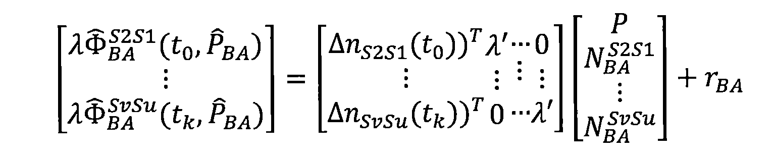
在一實施例中,該方法包括界定1110LS解估計及共變數矩陣。LS用以得知用於未知數之估計,以及共 變數估計。 In an embodiment, the method includes defining an 1110 LS solution estimate and a covariate matrix. LS is used to know the estimate for the unknown, and Variable estimate.
所得LS解估計之實例為
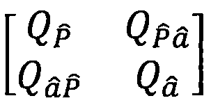
針對收斂或發散來檢查1112解。若不存在收斂或發散,則該方法返回至步驟1104。否則輸出1114解。 Check the 1112 solution for convergence or divergence. If there is no convergence or divergence, the method returns to step 1104. Otherwise output 1114 solution.
在一實施例中,昨天的最佳解估計用作用於浮動演算法之初始解。運用僅僅一次反覆來再次進行浮動演算法。若此解之包裝殘餘之均方誤差小於反覆浮動解之均方誤差,則輸出此解。 In an embodiment, the best solution estimate for yesterday is used as the initial solution for the floating algorithm. Use only one iteration to repeat the floating algorithm. If the mean square error of the package residue of this solution is less than the mean square error of the inverse floating solution, then the solution is output.
在一實施例中,固定模組406經組配以使用方位估計、模糊度估計及來自浮動區段的模糊度估計之共變數來改良浮動解之準確度。 In one embodiment, the fixed module 406 is configured to improve the accuracy of the floating solution using azimuth estimation, ambiguity estimation, and covariation of ambiguity estimates from the floating segments.
固定解固定整數N S ,亦被稱作固定整數模糊度,或僅僅固定模糊度。浮動解方法為線性方法,且因此,N S 在藉由LS方法予以求解時不為其應為之整數。 Fixed fixed integer N S , also known as fixed integer ambiguity, or only fixed ambiguity. The floating solution method is a linear method, and therefore, N S is not an integer that should be solved by the LS method.
若N S 可固定至正確整數,則未知數之數目自為方位向量加全部N S 縮減至僅僅方位向量。若N S 被設定為正確值,則此具有產生更準確解之潛在效應。 If N S can be fixed to the correct integer, the number of unknowns is reduced from the orientation vector plus all N S to only the orientation vector. If N S is set to the correct value, this has the potential effect of producing a more accurate solution.
為了固定模糊度,使用拉目達演算法經由ILS而將共變數以及自浮動解


接著可在以上方程式上使用LS以獲得固定解估計


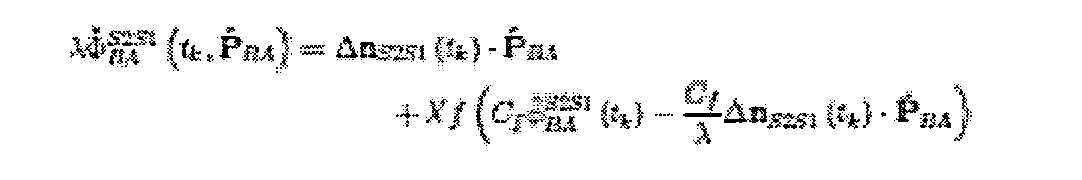
自以上方程式,LS可用以使用以下方程式來獲得解

此解亦為固定解,但在進行此捨位時,在解開的同時引入的任何循環滑移被移除,此係因為此捨位對於循環滑移係不變的。 This solution is also a fixed solution, but any loop slip introduced at the same time as the truncation is removed, because this truncation is constant for the cyclic slip system.
預期到,在給出實際真解的情況下的殘餘之均方誤差將產生用於全部給定解之最低值。由此,需要在固定演算法中包括一個最終步驟,藉以比較用於今天的最佳估計之殘餘之均方誤差與昨天的最佳估計。 It is expected that the residual mean square error given the actual true solution will produce the lowest value for all given solutions. Thus, a final step in the fixed algorithm is needed to compare the mean squared error for today's best estimate with yesterday's best estimate.
若使用昨天的最佳估計之殘餘之均方誤差 相比於使用今天的最佳估計之殘餘之均方誤差產生較低值,則此意謂出於任何原因而很可能使昨天的最佳估計相比於今天的當前估計為今天的較佳估計。在此狀況下,需要使用昨天的最佳估計而將雙差捨位至最近解平面,且接著使用最小平方以得知今天的新估計。 If using the best estimate of the mean square error of yesterday's best estimate Compared to the residual mean square error using today's best estimate yielding a lower value, this means that for any reason it is likely that yesterday's best estimate is compared to today's current estimate as today's better estimate. . In this case, it is necessary to use the best estimate of yesterday to round the double difference to the nearest solution plane, and then use the least square to know today's new estimate.
圖12展示由固定模組406實施之演算法之實例。方法1200檢查1202 


在一實施例中,在給出模糊度共變數


在一實施例中,該方法基於整數模糊度估計
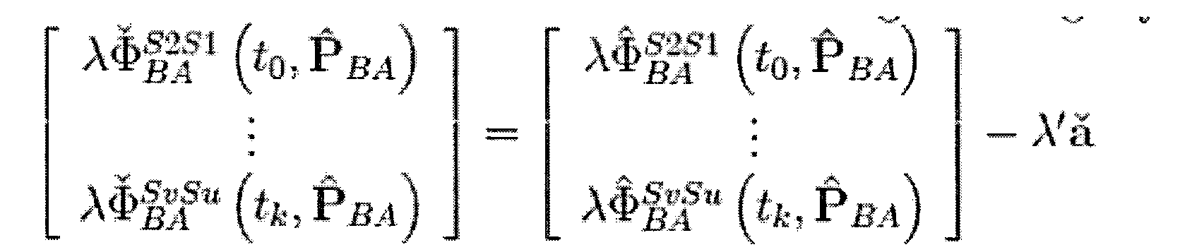
在一實施例中,該方法使用LS以獲得1208對以下方程式之第一解估計

在一實施例中,在給出解

在一實施例中,該方法使用LS以獲得1212對
以下方程式之第二解估計

在一實施例中,該方法比較使用昨天的最佳解估計P yesterday 的包裝殘餘之均方誤差與使用


在一實施例中,下文闡明每天恆星濾波方程式,其中下標n表示天n,條記號為遍及匹配雙差之天內的平均值,

已出於清晰起見而省略用於天內時間(同一天內之時間)、衛星及接收器命名法之全部記號。 All tokens for the time of day (time of the same day), satellite and receiver nomenclature have been omitted for clarity.

下文更完全地導出及探索以上方程式。 The above equations are derived and explored more fully below.
在一實施例中,恆星模組408經組配以進行恆星濾波,其中衛星群集大致每隔24小時246秒(亦被錯誤地稱作GPS恆星日)而重複。因為真實恆星日長度在地球上為大約24小時236秒,所以其係錯誤的。 In one embodiment, the star modules 408 are assembled for stellar filtering, wherein the satellite clusters are repeated approximately every 24 hours and 246 seconds (also incorrectly referred to as GPS stellar days). Because the real stellar day length is about 24 hours and 236 seconds on Earth, it is wrong.
若屬於一對衛星及一對接收器之雙差在時間上被分離整數數目個標稱GPS衛星軌道重複週期且在不同恆星日,則該等雙差被視為匹配。 If the double difference belonging to a pair of satellites and a pair of receivers is separated in time by an integer number of nominal GPS satellite orbit repeat periods and on different star days, then such double differences are considered to be matched.
因為多路徑隨GPS接收器之周圍環境及衛星幾何形狀而變,所以只要GPS接收器之周圍環境相對於GPS接收器不改變,則多路徑誤差就應自一個恆星日至下一恆星日幾乎相同。 Since the multipath varies with the surrounding environment of the GPS receiver and the geometry of the satellite, the multipath error should be almost the same from one stellar day to the next stellar day as long as the surrounding environment of the GPS receiver does not change relative to the GPS receiver. .
條記號為在可能時包括當前日n所計算之算術平均值。對於在日n的r k ,此為

為了計算恆星濾波解,需要計算


因此,代替直接計算(r n -


以此方式,(r n -
圖13展示由恆星模組408實施之方法1300之實例。首先藉由選擇P B 之值作為自固定模組獲得之第一一直固定解來初始化P B 之值。 FIG. 13 shows an example of a method 1300 implemented by a star module 408. First, the value of P B is initialized by selecting the value of P B as the first constant fixed solution obtained by the self-fixing module.
在一實施例中,該方法包括將包裝殘餘r k 暫時地移位1302a p 之整數倍以將其與今天(日n)對準。 In one embodiment, the method comprises packaging the residual r k is temporarily displaced 1302 a to an integer multiple of p is aligned with today (day n).
在一實施例中,方法1300判定1304有偏包裝殘餘。用以進行此功能之方程式之實例為:
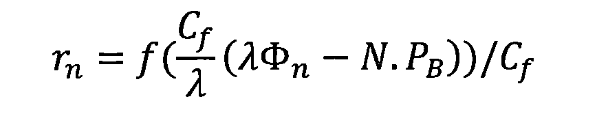
在一實施例中,該方法排除1306離群值。一種用於排除離群值之技術係自m日中排除全部日k,其中∥

在一實施例中,臨限值為大約1cm。在一實施例中,臨限值為大約2cm。 In an embodiment, the threshold is about 1 cm. In one embodiment, the threshold is about 2 cm.
在一實施例中,該方法判定或獲得1308平均值。平均值之一個實例為遍及來自m日之全部匹配雙差的全部|r k |之平均值以產生


在一實施例中,該方法判定1310估計。舉例
而言,
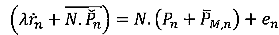

函數magmin(x,y)選擇具有最小絕對量值之自變數的傳回值。已確認,每一衛星重複週期隨衛星不同而不同。出於簡單起見,a p 之值被選擇為固定值,例如24小時246秒。 The function magmin(x, y) selects the return value of the argument with the smallest absolute magnitude. It has been confirmed that each satellite repetition period varies from satellite to satellite. For simplicity, the value of a p is chosen to be a fixed value, such as 24 hours and 246 seconds.
對於浮動階段及固定階段兩者,使用LS來求解線性方程式集合。因為在方程式中使用全部雙差的情況下可按照兩個其他雙差
在一實施例中,使用獨立集以避免此情形。為了決定哪些雙差被保留且哪些雙差被移除,使用參考衛星。參考衛星為必須在每一雙差中出現的每一曆元中之衛星。此產生雙差之星形型樣,其中已相對於此參考衛星而採取每一雙差。哪些參考衛星被使用可對方位解造成大的差異;此係因為參考衛星將其雜訊引入至方程式集合中之每一方程式中。 In an embodiment, an independent set is used to avoid this situation. In order to determine which double differences are retained and which double differences are removed, a reference satellite is used. The reference satellite is a satellite in each epoch that must appear in each double difference. This produces a double-difference star pattern in which each double difference has been taken with respect to this reference satellite. Which reference satellites are used can make a large difference to the azimuth solution; this is because the reference satellite introduces its noise into each of the equations in the equation set.
因此,將參考衛星選擇為具有最低雜訊之衛星會潛在地產生最準確解。選擇參考衛星之典型方法係歸因於具有高仰角之衛星具有低雜訊及低多路徑之假定而選擇具有最高仰角的衛星。 Therefore, selecting the satellite with the lowest noise from the reference satellite will potentially produce the most accurate solution. A typical method of selecting a reference satellite is to select the satellite with the highest elevation angle due to the assumption that the satellite with high elevation angle has low noise and low multipath.
參考衛星之選擇可變更最終解之準確度且對於基於精確差之解係關鍵的。演算法之固定階段及浮動階段兩者皆使用參考衛星之想法且使用同一獨立雙差集合。 The choice of reference satellites can change the accuracy of the final solution and is critical to solutions based on accurate differences. Both the fixed and floating phases of the algorithm use the idea of a reference satellite and use the same set of independent double differences.
相比於隨機地選擇參考衛星,選擇具有最高 仰角之衛星作為參考衛星會潛在地在全部方向上產生較小方差。 Compared to randomly selecting a reference satellite, the selection has the highest A satellite with an elevation angle as a reference satellite can potentially produce a smaller variance in all directions.
標題為「GPS基礎(GPS basics)」之附錄A提供基於GPS信號之背景閱讀。 Appendix A, entitled "GPS Basics", provides background reading based on GPS signals.
標題為「差分化相位可觀測量(Differencing the phase observable)」之附錄B闡釋解處理之更特定態樣。 Appendix B, entitled "Differencing the phase observable", explains the more specific aspects of the solution.
標題為「在夜晚之節點功能性(Node functionality at night)」之附錄C提供用以在夜晚獲得觀測之實驗之細節。 The details of the experiment used to obtain observations at night are provided in Appendix C entitled "Node functionality at night".
標題為「網路(Network)」之附錄D描述用以建立通訊網路之實施例的結構及演算法。 Appendix D, entitled "Network," describes the structure and algorithm for implementing an embodiment of a communication network.
標題為「第3章-多路徑及恆星濾波(Chapter 3-Multipath and sidereal filtering)」之附錄E描述既在已實施恆星濾波之前亦在已實施恆星濾波之後解在一實施例中採取的形式。 Appendix E, entitled "Chapter 3 - Multipath and sidereal filtering", describes the form taken in an embodiment both before and after the stellar filtering has been implemented.
標題為「第4章-演算法比較(Chapter 4-Algorithm comparison)」之附錄F比較使用上文所揭示之實施例而獲得的解與自其他解處理軟體獲得的解。 Appendix F, entitled "Chapter 4-Algorithm Comparison", compares the solutions obtained using the embodiments disclosed above with the solutions obtained from other solution processing software.
標題為「第6章-試驗台結果及分析(Chapter 6-Testbed results and analysis)」之附錄G描述兩個實驗之結果及分析。 The results and analysis of the two experiments are described in Appendix G entitled "Chapter 6 - Testbed results and analysis".
本發明之前述描述包括其較佳形式。可在不脫離如由隨附申請專利範圍所界定的本發明之範疇的情況下對該等較佳形式進行修改。 The foregoing description of the invention includes its preferred forms. Such preferred forms may be modified without departing from the scope of the invention as defined by the appended claims.
GPS基礎GPS foundation
在此附錄中,大體上介紹GPS操作,且尤其是與使用單頻帶接收器來獲取用於求解方位解之觀測相關的態樣。 In this appendix, GPS operations are generally described, and in particular, with the use of a single-band receiver to obtain aspects related to the observation of the azimuth solution.
A.1 GPS信號A.1 GPS signal
截至書寫為止,GPS當前正經歷現代化以改良民用用途及軍用用途兩者。在1990年與2004年之間發射了傳統衛星,而自2005年起已發射現代化衛星。根據國家空間定位、導航及定時協調辦公室[16],此致力於升級GPS之特徵及效能。當前,GPS在自衛星至終端使用者之三個不同RF鏈路上傳輸。RF鏈路被稱為L1、L2及L5,且在供其進行傳輸之頻帶之後被命名。分碼多重存取(CDMA)用作通道存取方法,因此全部衛星使用相同載波頻率。L1具有如自地球所見的1575.42Mhz之標稱頻率,L2具有1227.60Mhz之標稱頻率,且L5具有1176.45Mhz之標稱頻率。此等標稱頻率係運用各種信號予以調變以輔助導航。當前GPS現代化由以下各者組成:大體上改良硬體,以及添加在RF鏈路上發送之更多信號。當前在進行中之GPS現代化將花費許多年,且在L1上產生諸如L1C之信號的衛星被預期為直至2016年才發射,預期到大約2026年有24顆衛星[31]。因為吾人僅關注單頻帶接收器,此係因為其相比於多頻帶接收器較便宜且當前沒有新的現代化信號在L1上進行操作,所以吾人在此處將吾人之研究限定於傳統L1信號之研究。 As of writing, GPS is currently undergoing modernization to improve both civilian and military uses. Traditional satellites were launched between 1990 and 2004, and modern satellites have been launched since 2005. According to the National Space Positioning, Navigation and Timing Coordination Office [16], this is dedicated to upgrading the features and performance of GPS. Currently, GPS is transmitted over three different RF links from satellite to end users. The RF links are referred to as L1, L2, and L5 and are named after the frequency band for which they are transmitted. Code division multiple access (CDMA) channel access method used, so all of the satellites using the same carrier frequency. L1 has a nominal frequency of 1575.42 Mhz as seen from Earth, L2 has a nominal frequency of 1227.60 Mhz, and L5 has a nominal frequency of 1176.45 Mhz. These nominal frequencies are modulated using various signals to aid navigation. Current GPS modernization consists of substantially improving hardware and adding more signals sent over the RF link. The ongoing GPS modernization will take many years, and satellites that generate signals such as L1C on L1 are expected to be launched until 2016, with 24 satellites expected to be around 2026 [31]. Since we only focus on single-band receivers, because it is cheaper than multi-band receivers and there is currently no new modernization signal operating on L1, we limit our research to traditional L1 signals here. the study.

L1上之GPS傳統信號由以下各者組成:在1.023Mb/s下發送的被稱為C/A之粗略獲取偽隨機數(PRN)代碼、在10.23Mb/s下發送的在被加密的情況下被稱為Y之精確PRN代碼P,及在50b/s下發送的被稱為NAV之導航資料。兩個PRN代碼對於每一衛星係唯一的,且每一PRN代碼擴展導航信號。PRN代碼之位元亦被稱為碼片。L1由同相及正交分量組成。每一分量係使用二元相移鍵控(BPSK)作為其調變技術而被單獨地調變。一個調變器被供應來自P(Y)與NAV之模2加法的位元串,而另一調變器被供應來自C/A與NAV之模2加法的位元串。信號及載波頻率係自單一時間源導出且彼此同步,因此除了致使該等信號以較高位準彼此同步以外亦致使該等信號彼此位元定相。圖A.1描繪此等信號之產生的方塊圖。假定衛星時脈保持完美頻率,則衛星在時間t發送之瞬時L1波前W TX (t)可被書寫如下。 The GPS legacy signal on L1 consists of a coarsely obtained pseudo-random number (PRN) code called C/A transmitted at 1.023 Mb/s, which is transmitted at 10.23 Mb/s. The exact PRN code P, referred to as Y, and the navigation data called NAV transmitted at 50b/s. The two PRN codes are unique to each satellite system, and each PRN code extends the navigation signal. The bits of the PRN code are also referred to as chips. L1 consists of in-phase and quadrature components. Each component is individually modulated using binary phase shift keying (BPSK) as its modulation technique. One modulator is supplied with a bit string from the modulo 2 addition of P(Y) and NAV, and the other modulator is supplied with a bit string from the modulo 2 addition of C/A and NAV. The signals and carrier frequencies are derived from a single time source and are synchronized with each other, thus causing the signals to phase with each other in addition to causing the signals to be synchronized with one another at a higher level. Figure A.1 depicts a block diagram of the generation of these signals. Assuming that the satellite clock maintains a perfect frequency, the instantaneous L1 wavefront W TX ( t ) transmitted by the satellite at time t can be written as follows.

其中S(t)=NAV(t)(P(Y)(t)e i0+C(t)e iπ/2)為複合信號,C(t)為C/A代碼,P(Y)(t)為P(Y)代碼,NAV(t)為導航資料,


其中A RX 為接收振幅,且△t(t)為自在傳輸時間之衛星至在接收時間t之接收器的傳輸飛行時間。重要的是認識到,△t(t)並非在時間t之衛星與接收器之間的飛行時間,而是基於接收器看到其之時的飛行時間。其類似於飛機經過且吾人聽到飛機之聲音的時間滯後於飛機實際上所在之處。如由聽者所判定的來自飛機之聲音之飛行時間不同於吾人將根據相對於相同接收時間計算飛機實際上所在之處至使用者而得到的飛行時間。 Where A RX is the received amplitude and Δ t ( t ) is the transmission time of flight from the satellite at the time of transmission to the receiver at the time of reception t . It is important to recognize that Δ t ( t ) is not the time of flight between the satellite and the receiver at time t, but rather the time of flight when the receiver sees it. It is similar to the time when the airplane passes and the voice of the aircraft is heard by the plane. The flight time from the sound of the aircraft as determined by the listener is different from the flight time that the person will be based on calculating the actual location of the aircraft to the user relative to the same reception time.
A.2 GPS接收器對經接收W A.2 GPS receiver pair received W RXRX (t)信號做什麼( t ) what the signal does
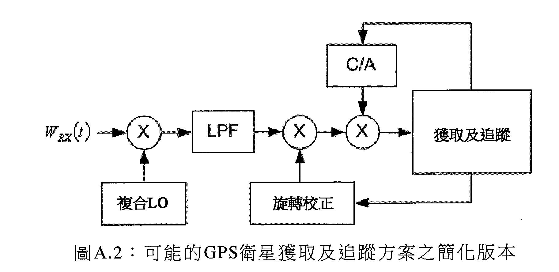
圖A.2展示GPS衛星接收器可做什麼以獲取衛星且追蹤其所產生之信號的簡化版本。在接收後,接收器就設法將信號與L1分離且追蹤C/A代碼及載波相位。此可藉由以下操作而有效地進行:將W RX (t)與複合本地振盪器

A.2.0.1 獲得基頻信號R(t)A.2.0.1 Obtain the fundamental frequency signal R ( t )
在與本地振盪器混頻且使用低通濾波器進行濾波之後,接收器獲得以下基頻,其中,△f=f RX -f TX 且
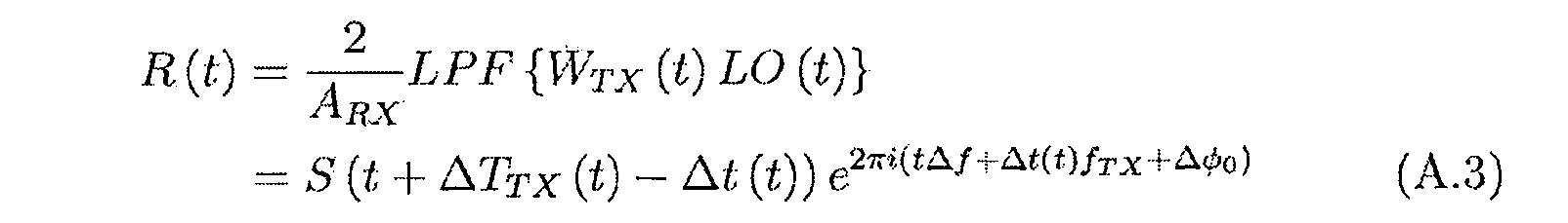
吾人將t△f+△t(t)f TX +△
A.2.0.2 停止旋轉A.2.0.2 Stop rotation
吾人看到,此為歸因於接收器之本地振盪器與衛星之振盪器之間的頻率差而旋轉及亦歸因於衛星自身相對於接收器之徑向運動而旋轉的四個點之群集。 As we have seen, this is a cluster of four points that are rotated due to the frequency difference between the local oscillator of the receiver and the oscillator of the satellite and also due to the radial movement of the satellite itself relative to the receiver. .
若吾人使
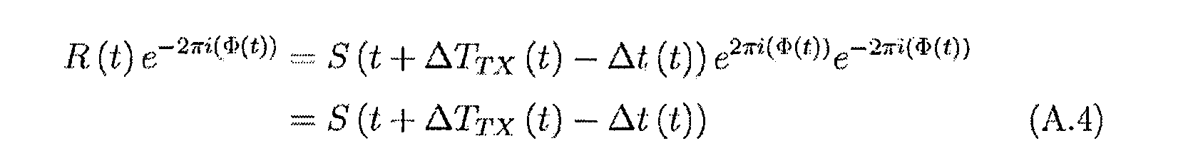
此阻止群集旋轉,且移除任何恆定群集旋轉偏移。此接著解析複合信號。因此,吾人將Φ(t)定義為接收器之經估計之經接收差拍載波相位(經估計載波相位)。群集之相位(或等效地為群集之旋轉偏移)被定義為載波相位與經估計載波相位之間的差t△f+△t(t)f TX +△
A.2.0.3 C/A代碼對準A.2.0.3 C/A code alignment
在已藉由使經估計載波相位與載波相位同相而停止群集旋轉之後,C/A代碼之本地複本必須與複合信號混頻且在時間上相移,直至C/A代碼之本地複本與經接收複合信號中之C/A代碼同相。吾人接著將τ(t)定義為C/A代碼對準偏移且為傳入C/A與本地複本未對準的程度。吾人將C/A代碼之本地複本定義為LCA(t)=C(t+△T RX (t)),其中△T RX (t)為接收器之時脈偏移。首先,吾人注意到,若吾人將本地C/A複本偏移τ(t)且使τ(t)=△t(t)+△T RX (t)-△T TX (t)並將此經 偏移C/A與R(t)相乘,則吾人針對隨機時間t預期下式。 After the cluster rotation has been stopped by causing the estimated carrier phase to be in phase with the carrier phase, the local replica of the C/A code must be mixed with the composite signal and phase shifted in time until the local replica of the C/A code is received. The C/A code in the composite signal is in phase. We then define τ ( t ) as the C/A code alignment offset and to the extent that the incoming C/A is misaligned with the local replica. We define the local replica of the C/A code as LCA ( t ) = C ( t + Δ T RX ( t )), where Δ T RX ( t ) is the clock offset of the receiver. First, we noticed that if we shift the local C/A replica by τ ( t ) and let τ ( t ) = Δ t ( t ) + Δ T RX ( t ) - Δ T TX ( t ) When the offset C/A is multiplied by R ( t ), then we expect the following equation for the random time t .

此係歸因於以下事實:P(Y)與C未很好地交叉相關,而當然C與其自身完美地相關。 This is due to the fact that P ( Y ) is not well cross-correlated with C , and of course C is perfectly related to itself.
LCA(t-τ(t))R(t)e -2πi(Φ(t))為至圖A.2中之獲取及追蹤區塊的輸入。在視覺上,LCA(t-τ(t))R(t)e -2πi(Φ(t))為在四個點無任何旋轉的情況下的群集。位於虛軸上之兩個點以一秒不大於50次緩慢地移動且含有導航資料,而位於實軸上之兩個點以均值為零之似隨機方式以一秒高達10.23百萬次極快速地移動。更一般而言,當發生此情形時,傳入C/A代碼與本地複本對準,且載波相位與經估計載波相位同相。 LCA ( t - τ ( t )) R ( t ) e -2π i (Φ( t )) is the input to the acquisition and tracking block in Figure A.2. Visually, LCA ( t - τ ( t )) R ( t ) e -2π i (Φ( t )) is a cluster without any rotation at four points. The two points on the imaginary axis move slowly with no more than 50 times per second and contain navigation data, while the two points on the real axis are in a random manner with a mean of zero, with a maximum of 10.23 million times per second. Move on the ground. More generally, when this occurs, the incoming C/A code is aligned with the local replica and the carrier phase is in phase with the estimated carrier phase.
A.3 獲取、追蹤及NAV資料提取A.3 Acquisition, tracking and NAV data extraction
A.3.0.1 使用濾波來提取NAV資料A.3.0.1 Using Filter to Extract NAV Data
當傳入C/A代碼與本地複本對準且載波相位與經估計載波相位同相時,可容易僅僅藉由使用低通濾波器來獲得導航資料NAV(t+△T TX (t)-△t(t))=-iLPF[LCA(t-τ(t))R(t)e -2πi(Φ(t))] (A.6) When the incoming C/A code is aligned with the local replica and the carrier phase is in phase with the estimated carrier phase, the navigation data NAV ( t + Δ T TX ( t ) - Δ t can be easily obtained simply by using a low pass filter. ( t ))=- iLPF [ LCA ( t - τ ( t )) R ( t ) e -2π i (Φ( t )) ] (A.6)
此允許GPS接收器存取包括大量資料的衛星之導航資料,該大量資料包括衛星之△T TX (t)估計及特定導航資料轉變之傳輸時間。以及用以計算衛星方位之資料。 This allows the GPS receiver to access navigation data for satellites including a large amount of data, including the Δ T TX ( t ) estimate of the satellite and the transmission time of the particular navigation data transition. And information used to calculate the position of the satellite.
A.3.0.2 用於C/A代碼對準及旋轉之度量A.3.0.2 Metrics for C/A code alignment and rotation
吾人將t限定為在小於NAV之週期的小時間段2δ內,同時仍確保足夠長週期,使得P(Y)與C遍及彼週期內仍未很好地相關。找到此時間段係可能的,此係因為NAV之週期比P(Y)之週期長204600倍。吾人假定C/A代碼完美地對準且載波相位與經估計載波相位同相。吾人接著預期下式。 We define t to be within a small time period 2 δ that is less than the period of the NAV , while still ensuring a sufficiently long period such that P ( Y ) and C are still not well correlated throughout the cycle. It is possible to find this time period because the period of the NAV is 204600 times longer than the period of P ( Y ). We assume that the C/A code is perfectly aligned and the carrier phase is in phase with the estimated carrier phase. I then expected the following formula.

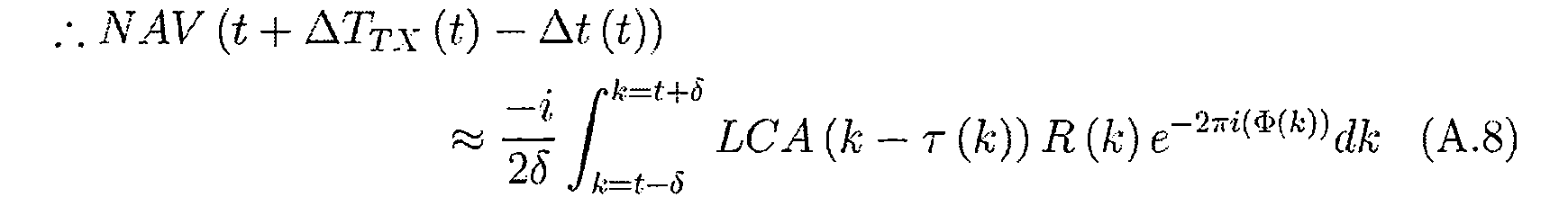
因為導航資料具有恆定量值1,所以歸因於不正確估計τ(t)的LCA(t-τ(t))與C(t+△T TX (t)-△t(t))之間的相關性之任何不完美性將影響所獲取導航資料之量值。另外,造成旋轉群集運動之不正確估計Φ(k)將在積分之後亦負面地影響所獲取導航資料之量值。因此,吾人可說明下式,其中γ被定義為C/A代碼之本地時移複本與經接收之可旋轉的C/A代碼之間的相關性係數。 Since the navigation data has a constant magnitude of 1, it is due to the incorrect estimation of τ ( t ) between LCA ( t - τ ( t )) and C ( t + Δ T TX ( t )-Δ t ( t )) Any imperfections in the relevance of the correlation will affect the magnitude of the navigation data obtained. In addition, an incorrect estimate of the rotational cluster motion Φ( k ) will also negatively affect the magnitude of the acquired navigation data after the integration. Therefore, we can specify the following equation, where γ is defined as the correlation coefficient between the local time-shifted replica of the C/A code and the received rotatable C/A code.

更一般而言,此係數可運用平均化予以更準確地計算;因此,GPS接收器可將其計算如下。 More generally, this coefficient can be calculated more accurately using averaging; therefore, the GPS receiver can calculate it as follows.

平方會消除BPSK之正負號。γ之量值與C/A代碼的對準程度及群集之旋轉運動的停止程度相關,而γ之角度與群集之具有半循環模糊度的恆定旋轉偏移相關。恆定群集旋轉 偏移不會影響γ之量值,此係因為恆定旋轉偏移剛好為可自積分中取出的常數。因此,當C/A代碼完美地對準且群集不旋轉時γ將被最大化,而γ對於群集之恆定旋轉偏移係不變的。 The square will eliminate the sign of BPSK. The magnitude of gamma is related to the degree of alignment of the C/A code and the degree of cessation of the rotational motion of the cluster, while the angle of gamma is related to the constant rotational offset of the cluster with half cycle ambiguity. Constant cluster rotation The offset does not affect the magnitude of gamma because the constant rotational offset is just a constant that can be taken from the integration. Therefore, γ will be maximized when the C/A code is perfectly aligned and the cluster is not rotating, while γ is constant for a constant rotational offset of the cluster.
˙當C/A代碼對準且群集不旋轉時|γ|被最大化。 | When the C/A code is aligned and the cluster is not spinning, |γ| is maximized.
在將Φ及τ視為變數的情況下,GPS接收器可變化Φ及τ以最大化γ。若γ高於某一臨限值,則GPS接收器可假定衛星被獲取且開始追蹤τ、Φ,並解碼NAV資料。 In the case where Φ and τ are considered as variables, the GPS receiver can vary Φ and τ to maximize γ. If γ is above a certain threshold, the GPS receiver can assume that the satellite is acquired and begins tracking τ, Φ, and decodes the NAV data.
吾人關注最大化γ,此係因為當γ為最大值時,在添加某一模糊度的情況下,Φ及τ兩者分別為t△f+△t(t)f TX +△
A.3.0.3 未知函數τ及Φ之一階線性近似A.3.0.3 One-order linear approximation of unknown function τ and Φ
吾人希望最大化相關性係數γ。歸因於γ相對於Φ及τ之量值之表面形狀,需要Φ及τ兩者之初始估計。在無良好初始估計的情況下,γ係由雜訊產生標準追蹤方案(諸如鎖相迴路(PLL)、鎖頻迴路(FLL)、延遲鎖定迴路(DLL)及早/晚時間無用)支配。其就像設法追蹤長草中之螞蟻爬行一樣;你必須在可追蹤螞蟻之前發現螞蟻,此係因為草使難以自遠處看到螞蟻。 We want to maximize the correlation coefficient γ. Due to the surface shape of gamma relative to the magnitude of Φ and τ, an initial estimate of both Φ and τ is required. In the absence of a good initial estimate, the gamma is dominated by noise generation standard tracking schemes such as phase-locked loops (PLLs), frequency-locked loops (FLLs), delay-locked loops (DLLs), and early/late time useless. It's like trying to track the ants crawling in the long grass; you have to find the ants before the ants can be traced, because the grass makes it difficult to see the ants from a distance.
首先,吾人建立Φ及τ如何改變之一階線性近似模型。吾人已經看到,當Φ(t)=t△f+△t(t)f TX +△


此等近似僅在F(t m )不快速地關於時間t m 改變的情況下才有效。速度將改變的最大速率為約0.1178ms -2且係衛星直接在頭頂之時(A.5.4)。在L1頻帶上,此暗示:若F(t m )在方程式A.13中保持不變,則群集旋轉速度將改變小於約0.9Hzs -1(參見A.5.3及A.5.4)。現在將此與F(t m )之範圍進行比較。△f TX (t m )可達約±5kHz(A.5.4),且取決於接收器時脈準確度,若吾人假定接收器時脈準確度為3.5ppm,則△f可超出另一5kHz。此意謂F(t m )之範圍為大約20kHz。若吾人將吾人之所關注時間限定於1ms,則F(t m )將改變小於0.0009Hz,其遠小於F(t m )的20kHz之範圍。因此,對於短時間段,此為有效近似。 These not only quickly approximate the time t m the case of a change to be effective in F (t m). The maximum rate at which the speed will change is approximately 0.1178 ms -2 and is when the satellite is directly overhead (A.5.4). In the L1 band, this implies that if F ( t m ) remains constant in Equation A.13, the cluster rotation speed will change by less than approximately 0.9 Hzs -1 (see A.5.3 and A.5.4). Now compare this to the range of F ( t m ). Δ f TX ( t m ) can reach approx. ±5 kHz (A.5.4), and depending on the receiver clock accuracy, if we assume that the receiver clock accuracy is 3.5 ppm , then Δ f can exceed the other 5 kHz . This means that F ( t m ) ranges from approximately 20 kHz . If we limit our attention time to 1 ms , F ( t m ) will change less than 0.0009 Hz , which is much smaller than the 20 kHz range of F ( t m ). Therefore, for a short period of time, this is a valid approximation.
方程式A.11及A.12形成Φ及τ將如何在短期內改變的近似模型。 Equations A.11 and A.12 form an approximate model of how Φ and τ will change in the short term.
A.3.0.4 關於獲取的未知函數τ及Φ之一階線性近似之進一步簡化A.3.0.4 Further simplification of the obtained one-order linear approximation of the unknown function τ and Φ
在圖A.2中,書寫如吾人已經看到的獲取及追蹤區塊之輸入,如在方程式A.13中。 In Figure A.2, write the input of the acquisition and tracking block as we have seen, as in Equation A.13.
LCA(t-τ(t))R(t)e -2πi(Φ(t)) (A.13) LCA ( t - τ ( t )) R ( t ) e -2π i (Φ( t )) (A.13)
為了獲取Φ及τ,吾人最初可對方程式A.11及A.12進行進一步簡化。方程式A.11中之θ(t m )在置放於方程式A.13中時對相對於時間改變群集旋轉沒有影響。A.13仍將為非旋轉四點群集,但僅僅具有θ(t m )循環之恆定旋轉偏移。如吾人已經在方程式A.10中所提及,任何恆定旋轉偏移對相關性係數之量值沒有影響。因此,吾人可在最初獲取Φ時忽略θ(t m )。 In order to obtain Φ and τ, we can further simplify the other programs A.11 and A.12. θ( t m ) in equation A.11 has no effect on changing cluster rotation with respect to time when placed in equation A.13. A.13 will still be a non-rotating four-point cluster, but with only a constant rotational offset of the θ( t m ) cycle. As we have already mentioned in Equation A.10, any constant rotational offset has no effect on the magnitude of the correlation coefficient. Therefore, we can ignore θ( t m ) when we initially acquire Φ.
載波頻率比C/A代碼之位元速率大1540倍。因為頻率乘時間為相位,所以若F=10,000Hz,則對於Φ而言,花費0.025ms而改變四分之一循環,而對於C/A代碼而言,花費38.5ms而改變四分之一碼片。若吾人接著假定R以4.092Mb/s之速率的數位化且取樣1ms R,則吾人甚至往往不能在C/A代碼中直接偵測F=0與F=10,000之間的差,而其將易於在載波中被偵測。 The carrier frequency is 1540 times larger than the bit rate of the C/A code. Since the frequency multiplication time is the phase, if F = 10,000 Hz , it takes 0.025 ms for Φ to change the quarter cycle, and for the C/A code, it takes 38.5 ms to change the quarter code. sheet. If it is then assumed at R / a rate of 4.092 Mb s and the digital sampling of 1 ms R, the I and often can not directly detect the difference between F 0 and F = = 10,000 in the C / A code, and which Easy to detect in the carrier.
歸因於此等兩個點,當考慮Φ及τ之初始獲取時吾人進行以下兩個近似。此處,吾人確認,群集將具有任意恆定旋轉偏移,僅在幾毫秒之時間段內才有效,且基頻取樣速率不大於每碼片幾次。 Due to these two points, when considering the initial acquisition of Φ and τ, we perform the following two approximations. Here, we confirm that the cluster will have any constant rotational offset, valid only for a period of a few milliseconds, and the base frequency sampling rate is no more than a few times per chip.
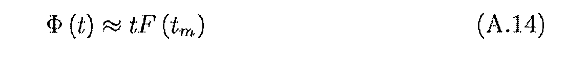

A.3.0.5 獲取A.3.0.5 Get
在此等兩個近似A.14及A.15的情況下,接收器可進行二維搜尋(F具有頻率維度且另一Ξ具有時間維度)以找到最大化方程式A.10中之相關性係數的點。假定接收器時脈準確度為3.5ppm,則接收器將必須自-10kHz搜尋至10kHz。因為C/A代碼為具有1ms週期之週期函數,所以接收器將必須自0ms搜尋至1ms。 In the case of these two approximations A.14 and A.15, the receiver can perform a two-dimensional search ( F has a frequency dimension and the other has a time dimension) to find the correlation coefficient in the maximum equation A.10. Point. It is assumed that the receiver clock accuracy is 3.5 ppm, the receiver would have to search from -10 kHz to 10 kHz. Since the C/A code is a periodic function with a 1ms period, the receiver will have to search from 0ms to 1ms.
藉由設法最大化本地C/A代碼複本與傳入C/A代碼之間的相關性來估計F及Ξ被證明為計算上要求使用比追蹤更多的能量,且為GPS接收器之主要關注。由此,已針對此問題進行許多研究以縮減用以估計此等兩個參數之計算努力[63]。藉由使用快速傅立葉變換(FFT)進行之並行化2D搜尋為當前在軟體界定接收器中使用之習知方法[63]。 Estimating F and Ξ by trying to maximize the correlation between the local C/A code replica and the incoming C/A code is proven to require computationally more energy than tracking, and is a primary concern for GPS receivers. . Thus, many studies have been conducted on this issue to reduce the computational effort to estimate these two parameters [63]. Parallelized 2D search by using Fast Fourier Transform (FFT) is a conventional method currently used in software-defined receivers [63].
作為一實例,吾人將本地C/A代碼複本與L1上之傳入C/A代碼複本交叉相關。吾人使用為碼片速率之標稱頻率之四倍的4.092Mb/s之取樣速率,並藉由以125Hz為步長將頻率項變化±10kHz且接著使用交叉相關而將時間項變化不大於±511.5碼片(±511.5碼片涵蓋整個1ms)進行搜尋。藉由使用隨機資料來模擬導航資料,而不添加P(Y)資料。將5000Hz之偏移應用於1.57542GHz載波頻率,且將250.15碼片之相位偏移應用於傳入信號之C/A代碼。在使用1ms之依序傳入資料的情況下,獲得圖A.3。 As an example, we cross-correlate the local C/A code replica with the incoming C/A code replica on L1. We use a sampling rate of 4.092 Mb/s which is four times the nominal frequency of the chip rate, and change the time term by no more than ±10 kHz by a frequency term of 125 Hz and then using cross-correlation A search of ±511.5 chips (±511.5 chips covering the entire 1 ms ). Simulate navigation data by using random data without adding P(Y) data. A 5000 Hz offset is applied to the 1.57542 GHz carrier frequency and a phase offset of 250.15 chips is applied to the C/A code of the incoming signal. Figure A.3 is obtained with a sequence of 1 ms incoming data.

如可看到,在表示F及Ξ之估計的圖形中存在清晰峰值。使用關於最高峰值之內插的經估計相位偏移為250.18碼片,而頻率之偏移為5000Hz;此與確切值很好地匹配。自此圖清晰地看到在t與Φ無良好初始估計的情況下追蹤為何將不起作用。值得指出的是,內插值超出之0.03碼片等於光行進9m所花費的時間。此大致為廉價消費等級GPS接收器所具有的正確準確度級。 As can be seen, there are clear peaks in the graphs representing the estimates of F and Ξ . The estimated phase offset using the interpolation for the highest peak is 250.18 chips , and the frequency offset is 5000 Hz ; this matches well with the exact value. It is clear from this figure that the tracking will not work if t and Φ have no good initial estimates. It is worth pointing out that the interpolated value exceeds 0.03 chips equal to the time it takes for the light to travel 9 m. This is roughly the correct level of accuracy that a low-cost consumer-grade GPS receiver has.
圖A.3中需要評估的點之數目為658,651。雖然較少點可能已被使用且仍能夠獲得F及Ξ之合理估計,但藉由2-D搜尋方法,始終固有地將存在大量需要評估的點。雖然存在諸如藉由使用FFT進行之並行化2D搜尋的其他方法且其計算上之要求較少及因此能量要求較少,但據吾人所知, 獲取仍使用比追蹤更多的能量。作為一實例,為現代消費等級GPS接收器之Ublox NEO-7N在其獲取狀態期間相比於其追蹤狀態使用多23%的能量[17]。 The number of points to be evaluated in Figure A.3 is 658,651. Although fewer points may have been used and still obtain reasonable estimates of F and Ξ , with the 2-D search method, there will always be a large number of points that need to be evaluated. While there are other methods such as parallelized 2D search by using FFT and their computational requirements are less and therefore less energy requirements, as far as we know, acquisition still uses more energy than tracking. As an example, the Ublox NEO-7N, which is a modern consumer grade GPS receiver, uses 23% more energy during its acquisition state than its tracking state [17].
A.3.0.6 追蹤A.3.0.6 Tracking
一旦已進行獲取且已找到最大相關性係數之點,接收器就接著可使用諸如PLL、FLL、DLL及早/晚追蹤方法之標準技術來追蹤τ及Φ。線性近似不會阻止最大相關性係數點移動,但線性近似充分地減緩該點移動,使得吾人可將其視為靜止點,直至其已被找到,接著,吾人可僅僅隨著該點移動而追蹤該點。 Once the acquisition has been made and the point of maximum correlation coefficient has been found, the receiver can then track τ and Φ using standard techniques such as PLL, FLL, DLL, and early/late tracking methods. The linear approximation does not prevent the maximum correlation coefficient point from moving, but the linear approximation sufficiently slows the point movement so that we can treat it as a stationary point until it has been found, and then we can only track as the point moves That point.
自獲取獲得F及Ξ之估計,其經由方程式A.12給出τ(t)之估計。為了追蹤τ(t),則可使用早/晚追蹤。此方法通常由三個本地產生之C/A複本組成,一個C/A複本稍微在自衛星預期者前面,一個C/A複本係如自衛星所預期,且一個C/A複本稍微在自衛星預期者後面。 An estimate of F and Ξ is obtained from the acquisition, which gives an estimate of τ( t ) via equation A.12. In order to track τ( t ), early/late tracking can be used. This method usually consists of three locally generated C/A replicas, one C/A replica slightly ahead of the satellite expectant, one C/A replica as expected from the satellite, and one C/A replica slightly from the satellite Behind the expectations.
早LCA(t-τ(t)+ξ) Early LCA ( t - τ ( t ) + ξ)
即時LCA(t-τ(t)) Instant LCA ( t - τ ( t ))
晚LCA(t-τ(t)-ξ) Late LCA ( t - τ ( t )-ξ)
接著使此等三個C/A複本各自與R(t)e -2πi(Φ(t))相關以產生三個相關性係數(γ E ,γ P ,γ L ),且在使用內插的情況下,可獲得τ(t)之新估計以使代碼保持對準。使代碼保持對準為用於最大化γ之兩個要求中的一者。 These three C/A replicas are then each correlated with R ( t ) e - 2π i (Φ( t )) to produce three correlation coefficients (γ E , γ P , γ L ), and interpolation is used. In the case, a new estimate of τ( t ) can be obtained to keep the code aligned. Keep the code aligned to one of the two requirements for maximizing gamma.
LCA(t-τ(t))R(t)具有自R移除C/A代碼之效應。此移除被稱為抹除代碼。一旦其被移除,就可在LCA(t-τ(t))R(t)上使用諸如PLL之載波追蹤方案,此係因為在一個方向上其表現為標準BPSK信號。可對LCA(t-τ(t))R(t)進行科斯塔斯(costas)PLL以估計Φ(t),此係因為其對於導航轉變係不變的。假定吾人設計科斯塔斯迴路以在虛軸上對準。接著,科斯塔斯迴路運用模糊度沿著虛軸對準NAV之BPSK信號,其對準係圍繞模糊度。科斯塔斯迴路亦將阻止群集旋轉,此為用於最大化γ之兩個要求中的一者。 LCA ( t -τ( t )) R ( t ) has the effect of removing the C/A code from R. This removal is called an erase code. Once it is removed, a carrier tracking scheme such as a PLL can be used on the LCA ( t - τ( t )) R ( t ) because it behaves as a standard BPSK signal in one direction. A costas PLL can be evaluated for LCA ( t - τ( t )) R ( t ) to estimate Φ( t ) because it is invariant to the navigation transition. Suppose we design a Costas loop to align on the imaginary axis. Next, the Costas loop uses the ambiguity to align the BPSK signal of the NAV along the imaginary axis, with the alignment around the ambiguity. The Costas loop will also prevent cluster rotation, which is one of two requirements for maximizing gamma.
因此,在同時使用代碼追蹤及載波追蹤的情況下,可連續地追蹤最大相關性點。對於接收器而言僅僅追蹤τ(t)或Φ(t)中之僅一者並不足夠;兩者需要被同時追蹤。 Therefore, in the case of using both code tracking and carrier tracking, the maximum correlation point can be continuously tracked. It is not sufficient for the receiver to track only one of τ( t ) or Φ( t ); both need to be tracked simultaneously.
吾人已經看到,在A.3.0.2中,τ(t)=△t(t)+△T RX (t)-△T TX (t)暗示最大相關性。歸因於1ms C/A模糊度,相反情形並不成立。因此,吾人可說最大相關性暗示τ(t)=△t(t)+△T RX (t)-△T TX (t)+M/1000,其中M為某一固定整數。 As we have seen, in A.3.0.2, τ ( t ) = Δ t ( t ) + Δ T RX ( t ) - Δ T TX ( t ) implies the maximum correlation. Due to the 1 ms C/A ambiguity, the opposite is not true. Therefore, we can say that the maximum correlation implies τ ( t ) = Δ t ( t ) + Δ T RX ( t ) - Δ T TX ( t ) + M / 1000, where M is a fixed integer.
同樣地,

當考慮此等模糊度時τ及Φ變成由幾乎全部低端消費等 級GPS接收器用於方位解計算的兩個可觀測量。 When considering these ambiguities, τ and Φ become almost all low-end consumption, etc. The level GPS receiver is used for two observable measurements of the azimuth solution calculation.
A.4 可觀測量A.4 Observable measurement
可觀測量為GPS接收器可直接量測之量的由GPS接收器採取之量測。可觀測量不會直接告知你GPS接收器位於何處,但藉由使用各種技術將允許你計算告知你GPS位於何處的方位解。吾人考慮的兩個可觀測量為代碼可觀測量及相位可觀測量。 Observable measurements are measurements taken by the GPS receiver that are directly measurable by the GPS receiver. Observables don't directly tell you where the GPS receiver is located, but using a variety of techniques will allow you to calculate the positional solution that tells you where the GPS is located. The two observables that we consider are code observable and phase observable.
吾人已藉由使用早晚定時及科斯塔斯PLL來追蹤γ之最大點而看到,吾人已找到針對某一固定整數M之τ(t)=△t(t)+△T RX (t)-△T TX (t)+M/1000及針對某一固定整數N之
A.4.1 代碼可觀測量A.4.1 Code observables
一旦追蹤到γ,接收器就可存取導航資料。導航資料以每字30位元被發送。在一子訊框中存在10個字,從而花費6秒進行傳輸。每一子訊框含有指示自衛星傳輸導航資料之第一位元的前緣之確切時間的交遞字(HOW)字。在衛星中,每一NAV資料轉變之第一位元對準至C/A代碼之第一碼片。此係可能的,此係因為C/A代碼及NAV資料係自同一振盪器導出(參見A.1)。圖A.4展示C/A NAV時序關係。 Once gamma is tracked, the receiver can access the navigation data. Navigation data is sent in 30 words per word. There are 10 words in a sub-frame, which takes 6 seconds to transmit. Each subframe contains a word of delivery (HOW) indicating the exact time of the leading edge of the first bit from the satellite transmission navigation data. In the satellite, the first bit of each NAV data transition is aligned to the first chip of the C/A code. This is possible because the C/A code and NAV data are derived from the same oscillator (see A.1). Figure A.4 shows the C/A NAV timing relationship.

因為每隔6秒之此唯一時戳及接收器連續地追蹤衛星之C/A代碼,所以C/A代碼之每一碼片可運用傳輸之確切時間予以唯一地識別。因此,接收器可求解代碼可觀測量中之模糊度M且因此可估計τ(t),使得τ(t)=△t(t)+△T RX (t)-△T TX (t)。 Since the unique time stamp and receiver continuously track the satellite's C/A code every 6 seconds, each chip of the C/A code can be uniquely identified using the exact time of transmission. Thus, the receiver may Ambiguity codes M of observables and thus may estimate τ (t), such that τ (t) = △ t ( t) + △ T RX (t) - △ T TX (t).
通常,代碼可觀測量係以公尺為單位且被稱為虛擬距離。藉由乘以光速c將τ(t)轉換成公尺會產生以下虛擬距離方程式,其中已出於簡潔起見而移除可變時間,且ρ為自在傳輸時間之傳輸器至在接收時間之接收器的距離。 Typically, code observables are measured in meters and are referred to as virtual distances. Converting τ( t ) into meters by multiplying the speed of light c produces the following virtual distance equation, where the variable time has been removed for the sake of brevity, and ρ is the transmitter of the free transmission time to the time of reception The distance of the receiver.
p=ρ+c(△T RX -△T TX ) (A.16) p = ρ + c (△ T RX -Δ T TX ) (A.16)
A.4.1.1 計算基於代碼之解A.4.1.1 Calculation based code solution
衛星之當前時脈偏差△T TX 係在導航資料中被傳輸且因此為已知值。因此,未知值為接收器之方位及時脈偏差;此等共同為P=[x,y,z,△T RX ]。此意謂虛擬距離為此等未知變 數之函數。獲得衛星之一個此類虛擬距離會產生以下非線性方程式。 The current clock offset ΔT TX of the satellite is transmitted in the navigation data and is therefore a known value. Therefore, the unknown value is the receiver's azimuth and time pulse deviation; these are collectively P = [ x , y , z , Δ T RX ]. This means that the virtual distance is a function of such unknown variables. Obtaining one such virtual distance of a satellite produces the following nonlinear equation.

因為求解線性方程式之簡易性,使用一階泰勒展開式來線性化此方程式對於導出求解任意大小之虛擬距離集合的一般化方法係明智的。吾人使經估計解為針對接收時間
之

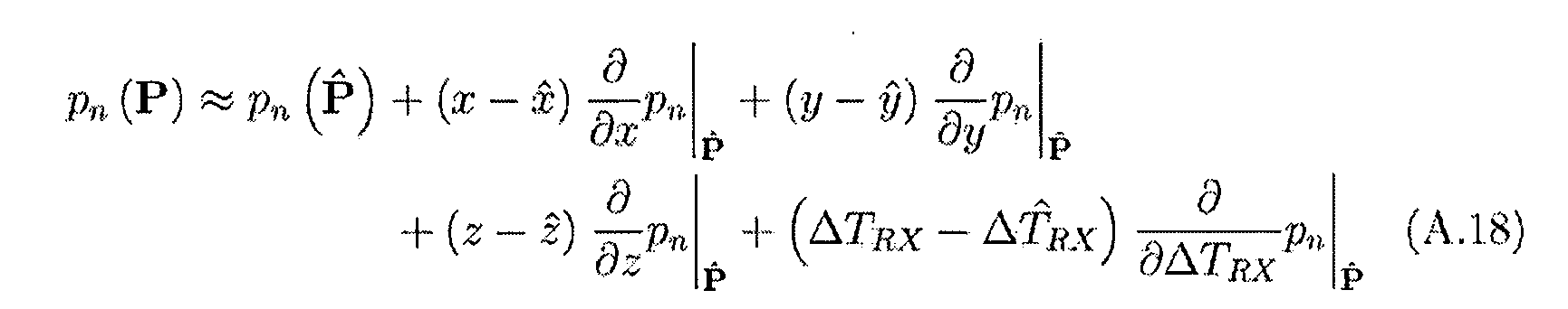
在給出針對虛擬距離p n 在傳輸時間的衛星之方位S n =[x n ,y n ,z n ]的情況下,則可在給出ρ n (x,y,z)=
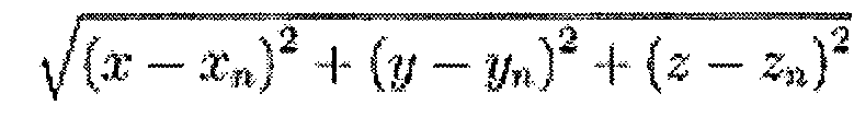

在給出良好估計

因為方程式A.19係線性的,所以此虛擬距離集合可以矩陣形式被書寫如下。 Since equation A.19 is linear, this virtual distance set can be written as a matrix as follows.

在使用粗體記號向量或矩陣的情況下,此具有A(P-


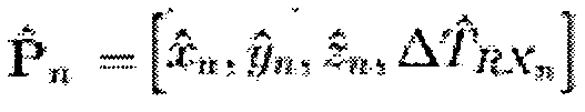


咸信由接收器T RX 在步驟3中產生接收時間之估計而對接收時間進行的校正對於大部分接收器而言將大約小於一毫秒且可以忽略。如步驟5中進行的計算傳輸時間之估計所需要的校正一般比較大,且大約為60ms,此係自衛星至接收器之近似飛行時間;此步驟不可忽略。 The receiver T RX generates an estimate of the reception time in step 3 and the correction of the reception time will be less than one millisecond for most receivers and can be ignored. The correction required to calculate the estimated transmission time as performed in step 5 is generally large and is approximately 60 ms , which is the approximate time of flight from the satellite to the receiver; this step is not negligible.
圖A.5展示針對六個衛星之集合及自其採取的代碼觀測的演算法A.1收斂之實例。如可看到,使用地球之中心作為六個反覆內之初始估計,演算法已收斂。 Figure A.5 shows an example of algorithm A.1 convergence for a set of six satellites and code observations taken from it. As can be seen, using the center of the Earth as the initial estimate within six replicates, the algorithm has converged.
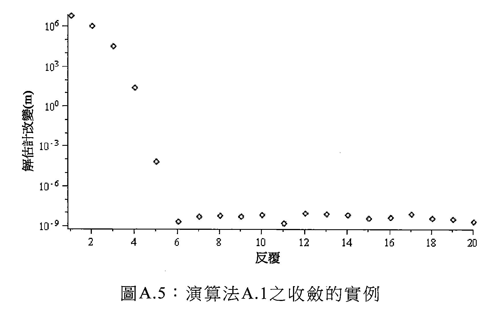
圖A.5中之實例的此演算法的輸出產生-116.644μs之接收器時脈偏差估計。此與如由接收器自身計算的-116.738μs之估計比較,兩者之間具有32m之空間解差異。 The output of this clock offset estimation algorithm of the example in Figure A.5 -116.644 μs of the receiver is generated. This is compared to an estimate of -116.738 μs as calculated by the receiver itself with a spatial solution difference of 32 m between the two.
A.4.1.2 最終代碼可觀測量模型A.4.1.2 Final code observables model
為何在吾人之解與如由GPS接收器自身計算的解之間存在32m之差異的一個原因係吾人已在方程式A.16的吾人之模型中忽略一些事物。方程式A.16中之模型可藉由添加 對流層延遲T、電離層延遲I、多路徑M r 及雜項誤差e r而延伸。因此,可書寫相位可觀測量之更確切模型,如在以下方程式中。 One reason why there is a difference of 32 m between our solution and the solution calculated by the GPS receiver itself is that we have ignored some things in the model of our equation A.16. A.16 in the model equation by adding tropospheric-delay T, the ionosphere delay I, M r multipath and miscellaneous error e r extends. Therefore, a more accurate model of phase observables can be written, as in the equation below.
p=ρ+c(△T RX -△T TX )+T+I+M r +e r (A.22) p = ρ + c (△ T RX - Δ T TX ) + T + I + M r + e r (A.22)
在誤差源之中,電離層通常係最大的。電離層在地球上方50km延伸至1000km,其主要由帶電粒子、帶電原子及帶電分子組成。大部分電離係由來自太陽之紫外線(UV)射線所引起且因此總電子計數(TEC)存在大的日改變,此改變又影響電離層校正項I。電離層可產生少至1m至高達100m之衛星距離誤差[13]。電離層校正項係頻率相依的且在雙頻帶接收器的情況下,可觀測量之電離層自由組合係可能的。對於單頻帶接收器,可能無此組合,實際上Klobuchar電離層模型用於單頻帶接收器GPS。Klobuchar係數係在導航訊息中傳輸,使得接收器接著可估計電離層校正項。Klobuchar演算法校正約50%之電離層誤差[40]。 Among the sources of error, the ionosphere is usually the largest. The ionosphere extends from 50km to 1000km above the Earth and consists mainly of charged particles, charged atoms and charged molecules. Most of the ionization system is caused by ultraviolet (UV) rays from the sun and thus there is a large daily change in the total electron count (TEC), which in turn affects the ionospheric correction term I. The ionosphere can produce satellite distance errors as small as 1m up to 100m [13]. The ionospheric correction term is frequency dependent and in the case of a dual band receiver, an observable ionospheric free combination is possible. For single-band receivers, there may be no such combination, in fact the Klobuchar ionospheric model is used for single-band receiver GPS. The Klobuchar coefficients are transmitted in the navigation message so that the receiver can then estimate the ionospheric correction term. The Klobuchar algorithm corrects about 50% of the ionospheric error [40].
此章節中對於吾人而言重要事物係吾人能夠獲得近似解、具有小於100m之某種準確度之空間分量,及某種小於1ps之時間準確度。關於代碼可觀測量,以上係吾人所關注的全部。 The important things in this chapter for us are that we can get an approximate solution, a spatial component with some accuracy of less than 100 m , and some time accuracy of less than 1 ps . Regarding the observable measurement of the code, the above are all of our concerns.
A.4.2 相位可觀測量A.4.2 Phase observables
相位可觀測量為由GPS接收器在特定時間內針對特定衛星所採取的量測之量。與僅使用代碼可觀測量進行量測之準確度相比較,相位可觀測量允許進行更高準確度GPS量測。此係歸因於與代碼可觀測量之碼片長度相比較的 GPS載波之短得多的波長。與C/A信號之碼片之大約300m長度相比較,L1之波長大約為20cm且可引起準確度之對應大的增加。量測來自監測接收之衛星載波與GPS接收器上之參考振盪器之間的相位差。接收器藉由追蹤而累積此瞬時相位差並將此作為相位可觀測量輸出至使用者。圖A.6展示在忽略在載波上發送的全部信號(諸如C/A、導航及P(Y)碼)的情況下在觀測衛星時GPS接收器正對於相位可觀測量進行什麼之方塊圖。 The phase observable is the amount of measurement taken by the GPS receiver for a particular satellite at a particular time. Phase observables allow for higher accuracy GPS measurements compared to the accuracy of measurements using only code observables. This is due to the comparison with the chip length of the code observable A much shorter wavelength of the GPS carrier. The wavelength of L1 is approximately 20 cm compared to the length of the chip of the C/A signal of approximately 300 m and can cause a correspondingly large increase in accuracy. The phase difference between the satellite carrier on the monitored receiver and the reference oscillator on the GPS receiver is measured. The receiver accumulates this instantaneous phase difference by tracking and outputs this as a phase observable to the user. Figure A.6 shows a block diagram of what the GPS receiver is doing for phase observables when observing satellites, ignoring all signals transmitted on the carrier, such as C/A, navigation, and P(Y) codes.

對於GPS,為了使GPS起作用,相位習慣以循環為單位而非弧度或度。相位為接收循環單位之三角函數內部之自變數。Φ S 為衛星之載波的相位,而Φ U 為接收器之參考相位。Φ S 及Φ U 兩者可變得任意大。 For GPS, in order for GPS to work, the phase is used in cycles rather than radians or degrees. The phase is the self-variable inside the trigonometric function of the receiving cycle unit. Φ S is the phase of the carrier of the satellite, and Φ U is the reference phase of the receiver. Both Φ S and Φ U can be arbitrarily large.
相位之累積中固有的係取決於你開始累積相位之時的模糊度N。除了模糊度以外亦存在遺漏一些旋轉之可能性。計數汽車輪胎旋轉之次數取決於你開始計數其旋轉之 時且亦取決於你是否遺漏任何旋轉。雖然GPS接收器設法連續地追蹤相位,但此未必總是可能的。歸因於雜訊、信號之損失或關斷GPS接收器及再次接通GPS接收器,相位之追蹤可丟失,從而引起N值的整數改變。此產生所謂的「循環滑移」。因此,理想地,此相位模糊度在衛星被追蹤的同時應為固定的,但歸因於循環滑移其偶爾地將改變。 The inherent in the accumulation of phases depends on the ambiguity N at which you begin to accumulate phases. In addition to the ambiguity, there is also the possibility of missing some rotation. Counting the number of times a car tire spins depends on when you start counting its rotation and also if you miss any rotation. Although the GPS receiver manages to continuously track the phase, this is not always possible. Due to noise, loss of signal, or turning off the GPS receiver and turning the GPS receiver back on, phase tracking can be lost, causing an integer change in the value of N. This produces a so-called "loop slip". Therefore, ideally, this phase ambiguity should be fixed while the satellite is being tracked, but it will occasionally change due to cyclic slip.
如吾人已看到,衛星不會發送出連續波,該等波係以兩個BPSK信號於一調變,一個信號在正交相位中且另一信號在同相中。碼追蹤具有自BPSK信號中之一者抹除C/A代碼的效應,但當設法追蹤其時仍使導航添加複雜度之位準。當BPSK資料不用以再生原始載波時,載波相位中之半循環模糊度被引入至相位可觀測量中且據說相位可觀測量具有為2之代碼因數C f =2。當BPSK資料用以再生原始載波時,原始載波可運用一個循環之模糊度完全再生且據說相位可觀測量具有為2之代碼因數C f =1。因此,當使用為1之代碼因數時可縮減相位可觀測量之模糊度。 As we have seen, the satellite does not transmit continuous waves, which are modulated by two BPSK signals, one in the quadrature phase and the other in the same phase. Code tracking has the effect of erasing the C/A code from one of the BPSK signals, but still adds a level of complexity to the navigation when trying to track it. When the phase observables BPSK data is not used for the reproduction of the original carrier, in the semi-circular carrier phase ambiguity is introduced and is said to have a code phase observable factor of 2 C f = 2. When the BPSK data for reproducing the original carrier, the carrier can use the original cycle ambiguity of a complete regeneration phase observables and said to have the code 2 of the factor C f = 1. Therefore, when a code factor of 1 is used, the ambiguity of the phase observable can be reduced.
A.4.2.1 最終相位可觀測量模型A.4.2.1 Final phase observables model
如吾人已看到,追蹤載波相位會最大化γ,其又意謂在追蹤的同時累積之相位在使用科斯塔斯PLL時對於某一固定整數N為

假定接收器之時脈係基於其本地振盪器且其頻率保持完美的時間,則真實GPS時間可經轉換為如由接收器判定
為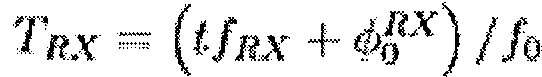


使兩式相減且乘以f 0會產生下式。 Subtracting the two equations and multiplying f 0 produces the following equation.

在使此式與方程式A.23相等的情況下,吾人看到,吾人可將方程式A.23書寫如下

f TX 為GPS傳輸器之振盪器且為極接近於f 0之原子時脈。因此,出於吾人之目的,f TX /f 0=1,且吾人可將方程式A.27重寫如下。 f TX is the oscillator of the GPS transmitter and is an atomic clock that is very close to f 0 . Therefore, for my purposes, f TX / f 0 =1, and we can rewrite equation A.27 as follows.
Φ=f 0(△T RX -△T TX )+ρ/λ0+N/C f (A.28) Φ= f 0 (△ T RX -Δ T TX )+ ρ /λ 0 + N / C f (A.28)
方程式A.28中之此模型可藉由如運用代碼可觀測量進行的添加對流層延遲T、電離層延遲I、多路徑


方程式A.29中之距離項p係針對在接收時間t RX 處之接收器及在傳輸時間t TX 處之衛星。因此,因為t TX 為比t RX 之當前時間早的時間,所以距離ρ為你所在之處至在短時間段之前衛星所在之處的量度;此等兩個值之間的差通常為約60ms標記且衛星可在此時間中移動幾百公尺。 The distance term p in equation A.29 is for the receiver at reception time t RX and the satellite at transmission time t TX . Therefore, since t TX is a time earlier than the current time of t RX , the distance ρ is a measure of where the satellite is from where you are until a short period of time; the difference between these two values is typically about 60 ms Mark and the satellite can move a few hundred meters during this time.
相位可觀測量係在GPS時間t RX 量測,此變數自身必須被求解,此係因為你不確切地知曉進行量測在什麼時間;你知曉你現在進行量測,但你不知曉現在為何時。此可使用如前所示之代碼可觀測量而獲得。 Phase observables are measured at GPS time t RX and this variable must be solved by itself, because you don't know exactly when to take the measurement; you know that you are measuring now, but you don't know when it is. This can be obtained using a code observable as shown previously.
接收器之時脈偏差係在t RX ,而衛星之時脈偏差係在t TX ,但此等並不如此關鍵,此係因為此等不在60ms內快速改變且可安全地假定為在短時間段內恆定。 The receiver's clock skew is at t RX , and the satellite's clock bias is at t TX , but this is not so critical, because it does not change quickly within 60ms and can safely be assumed to be in a short period of time. Constant inside.
方程式A.29為用於相位可觀測量之吾人之最終模型。左側為接收器給予吾人之物,而右側為吾人將其解譯為之物。將其乘以衛星之標稱波長仍分類為單差,而非相位可觀測量之循環的單位,相位可觀測量單位變成公尺。 Equation A.29 is the final model for our phase observables. On the left is what the receiver gives to us, and on the right is what we interpret as something. Multiplying it by the nominal wavelength of the satellite is still classified as a single difference, rather than the unit of the cycle of phase observable measurement, and the phase observable unit becomes a meter.
A.5 選定證明A.5 Certificate of choice
A.5.1 使用飛行時間近似之經接收相位A.5.1 Received phase using time-of-flight approximation
飛行時間之泰勒展開式

一階線性近似
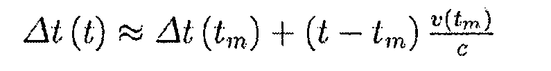
定義經接收相位

A.5.2τ 一階線性近似A.5.2τ First-order linear approximation
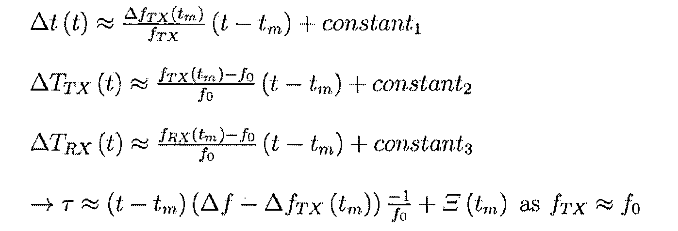
A.5.3 具有恆定徑向速度偏移 
恆定速度偏移發生了什麼。 What happens to the constant speed offset.
若徑向速度一直超出

其中θ'(t m )及δ為一些常數 Where θ ' ( t m ) and δ are some constants
A.5.4 衛星相對於接收器之最大徑向速度及加速度A.5.4 Maximum radial velocity and acceleration of the satellite relative to the receiver
圖A.7為衛星在傳輸至接收器的同時圍繞地球運行的簡化模型。不考慮相對論效應且假定衛星之軌道極佳地為具有恆定切向速度之圓形且當衛星最接近接收器時衛星直接在頭頂。 Figure A.7 is a simplified model of the satellite orbiting the Earth while transmitting to the receiver. The relativistic effect is not considered and it is assumed that the orbit of the satellite is excellently circular with a constant tangential velocity and that the satellite is directly overhead when the satellite is closest to the receiver.

自圖A.7吾人獲得描述系統之以下方程式。 From Figure A.7, we have the following equations describing the system.
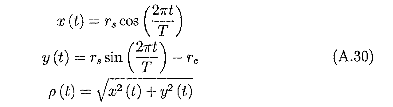
使用以下近似值,近似值為GPS衛星軌道週期T、地球之半徑及GPS衛星軌道之半徑的大體上認可之值。藉由區分距離方程式A.30,獲得圖A.8。 Using the approximate values below, the approximation is a generally accepted value for the GPS satellite orbital period T , the radius of the Earth, and the radius of the GPS satellite orbit. Figure A.8 is obtained by distinguishing the distance equation A.30.
T e =6371000m T s =26600000m T=43080s (A.31) T e = 6371000 m T s = 26600000 m T= 43080 s (A.31)

自模型導出的最大徑向速度在衛星上升時間及設定時間為929ms -1 。最大加速度為0.1178ms -2 且係在衛星直接在頭頂之時。[57](第91頁)陳述GPS衛星可具有相對於地球上之靜止接收器的高達800ms -1 之徑向速度。此與吾人之簡化模型一致。在L1頻帶上,0.1178ms -2 之加速度大約為0.9Hzs -1都卜勒頻移率,而L1頻帶上之929ms -1 大約為5kHz都卜勒頻移,因此f 0 ±5kHz必須經搜尋用於載波頻率。 The maximum radial velocity derived from the model is 929 ms -1 at satellite rise time and set time. The maximum acceleration is 0.1178 ms -2 and is when the satellite is directly above the head. [57] (p. 91) states that GPS satellites can have radial velocities of up to 800 ms -1 relative to stationary receivers on Earth. This is consistent with our simplified model. In the L1 band, the acceleration of 0.1178 ms -2 is about 0.9 Hzs -1 Doppler shift rate, while the 929 ms -1 on the L1 band is about 5 kHz Doppler shift, so f 0 ±5 kHz must pass Search for carrier frequency.
差分化相位可觀測量Differential phase observable
使用多個相位觀測並採取其之差會產生可用於得知方位解的各種差。在此附錄中吾人查看此等差及方位解採用的何種形式。 Using multiple phase observations and taking the difference produces a variety of differences that can be used to learn the azimuth solution. In this appendix we see which form of this difference and orientation solution is used.
B.1 單差B.1 single difference
單差為兩個不同GPS接收器(兩個不同使用者)在同一曆元處的兩個相位可觀測量之間的差。進行單差消除在觀測一個衛星時之系統誤差。此等誤差包括衛星時脈偏差及在很大程度上大氣壓誤差。 The single difference is the difference between two phase observables at the same epoch for two different GPS receivers (two different users). Perform a single difference to eliminate systematic errors in observing a satellite. These errors include satellite clock skew and, to a large extent, atmospheric pressure errors.
吾人現在使用兩個GPS接收器A及B以觀測衛星S。相位可觀測量係在大約相同時間藉由兩個接收器量測。使用者A報告如由接收器自身上之系統時脈報告的時間T A ,而使用者B報告在採取其量測時其GPS接收器上之時脈為T B。實際GPS時間與根據接收器自身上之時脈的時間之間的關係如下。 We now use two GPS receivers A and B to observe satellite S. Phase observables are measured by two receivers at approximately the same time. User A reports the time T A as reported by the system clock on the receiver itself, and User B reports that the clock on its GPS receiver is T B when taking its measurements. The relationship between the actual GPS time and the time according to the clock on the receiver itself is as follows.
t A =T A -△T A (B.1) t A = T A -△ T A (B.1)
t B =T B -△T B (B.2) t B = T B -△ T B (B.2)
在使用虛擬距離可觀測量的情況下,可獲得接收器時脈偏差△T a 及△TB。小於1ps的時脈偏差之良好估計被假定為今後給出。 In the case of using a virtual distance observable, the receiver clock offsets Δ T a and ΔT B can be obtained. A good estimate of the clock skew less than 1 ps is assumed to be given in the future.
兩個可觀測量模型可被書寫如下,其中應理解,多路徑誤差及雜項誤差指代相位可觀測量而非代碼。 Two observable models can be written as follows, where it should be understood that multipath errors and miscellaneous errors refer to phase observables rather than code.

其中△T S 為衛星之時脈偏差,T為對流層校正,I為電離層校正,C f 為代碼因數,


雖然對流層校正及電離層校正對於兩個接收器不完全地相同,但吾人假定其係完全地相同。亦因為量測並非完全同時進行,所以衛星時脈偏差在兩個接收器採取量測時將係不同的,但此處吾人假定衛星時脈偏差△T S 對於兩個接收器係相同的。 Although tropospheric correction and ionospheric correction are not completely identical for the two receivers, we assume that they are completely identical. Also because the measurements are not completely simultaneous, the satellite clock bias will be different when the two receivers are taking measurements, but here we assume that the satellite clock offset Δ T S is the same for both receivers.
因為觀測並非同時,所以兩個使用者在不同地點看到衛星;下圖描述該情形。 Since the observations are not simultaneous, two users see the satellite at different locations; the following figure describes the situation.
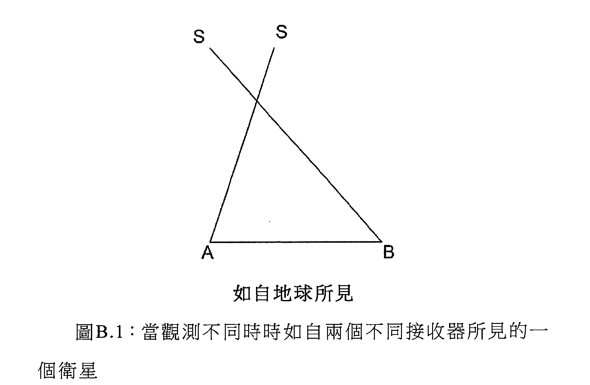
吾人因此外推第二t上之共同曆元。吾人現在必須調整相位可觀測量如同吾人實際上在此共同曆元處採取量測。為了做到這一點,吾人可在兩個距離項上使用使用泰勒展開式的一階近似並重排其得到下式。 We therefore extrapolated the common epoch on the second t . We now have to adjust the phase observables as we actually take measurements at this common epoch. In order to do this, we can use the first-order approximation using Taylor expansion on two distance terms and rearrange them to get the following formula.
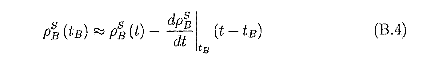


在將此回代至方程式B.3中之可觀測量模型中的情況下,吾人得到下式。 In the case where this is substituted into the observable model in Equation B.3, we obtain the following formula.

距離變化率


若吾人假定接收器大體上靜止且距離變化率比光速小得多,則吾人獲得下式。 If we assume that the receiver is substantially stationary and the rate of change of distance is much smaller than the speed of light, then we obtain the following equation.

如吾人已看到的最大距離變化率小於800ms -1 ,其比光速小得多,因此其為有效假定。通常,t-t B 將比1ms小得多,1ms將在方程式B.5中產生小於10μm之校正誤差,其為可接受的誤差。 As we have seen, the maximum distance change rate is less than 800 ms -1 , which is much smaller than the speed of light, so it is a valid assumption. In general, t - t B will be much smaller than 1 ms , and 1 ms will produce a correction error of less than 10 μm in equation B.5, which is an acceptable error.
方程式B.5的左側之項係全部可獲得的。Φ為在吾人已選擇的共同曆元t之經量測相位可觀測量,量測之實際時間t B 係已知的且吾人亦可估計距離變化率。左側為相位可觀測量之校正版本以考量相位可觀測量並非同時採取的事實。吾人因此將給定之相位可觀測量重寫如下。 The items on the left side of equation B.5 are all available. Φ is the measured phase observable of the common epoch t that we have selected. The actual time t B of the measurement is known and we can also estimate the rate of change of the distance. The left side is the corrected version of the phase observable to take into account the fact that phase observables are not taken at the same time. We therefore rewrite the given phase observables as follows.
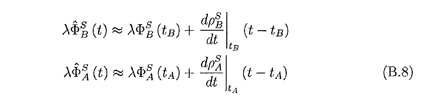
Φ符號之頂部上的上標三角將展示吾人此時並未量測相位,而實際上其為其在彼時的估計。比如t與t A 之間的時差很可能小於一毫秒,一毫秒對於吾人此處談論之時間係相對短的時間段且因此為可接受之近似值。在將方程式B.8代入至方程式B.3中後,吾人就得到外推至共同曆元t之以下相位可觀測量。 The superscript triangle on top of the Φ symbol will show that we have not measured the phase at this time, but in fact it is an estimate of it at that time. For example the difference between t A and t is likely less than one millisecond, a millisecond for time-based I here talking about the relatively short period of time and is therefore acceptable approximation. After substituting equation B.8 into equation B.3, we are extrapolated to the following phase observables of the common epoch t .

在採取方程式B.9中之兩個可觀測量之間的差的情況
下,吾人得到下式,其中
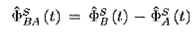

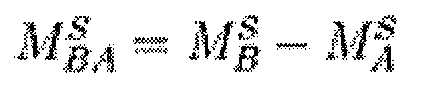
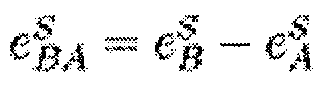
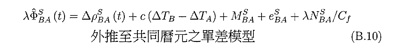
此單差具有移除兩個接收器共同之誤差的效應。此等誤差包括大氣壓誤差及與衛星自身相關的誤差。假定兩個接收器足夠接近,使得大氣條件對於兩個使用者相同且此等兩個觀測之間的時間儘可能地小。然而,亦不考量多路徑及雜項誤差(諸如雜訊)。 This single difference has the effect of removing the error common to both receivers. These errors include atmospheric pressure errors and errors associated with the satellite itself. It is assumed that the two receivers are close enough that the atmospheric conditions are the same for both users and the time between these two observations is as small as possible. However, multipath and miscellaneous errors (such as noise) are not considered.
B.1.1單差解譯B.1.1 single difference interpretation
吾人現在進行如下近似:與兩個接收器彼此相距距離相比較,衛星距接收器距離要遠得多。此意謂衛星幾乎在距接收器無限遠處出現,此意謂角度SAB等於角度ABS,如下圖所描繪。 We now make the following approximation: the satellite is much farther away from the receiver than the distance between the two receivers. This means that the satellite appears almost infinity from the receiver, which means that the angle SAB is equal to the angle ABS, as depicted in the following figure.
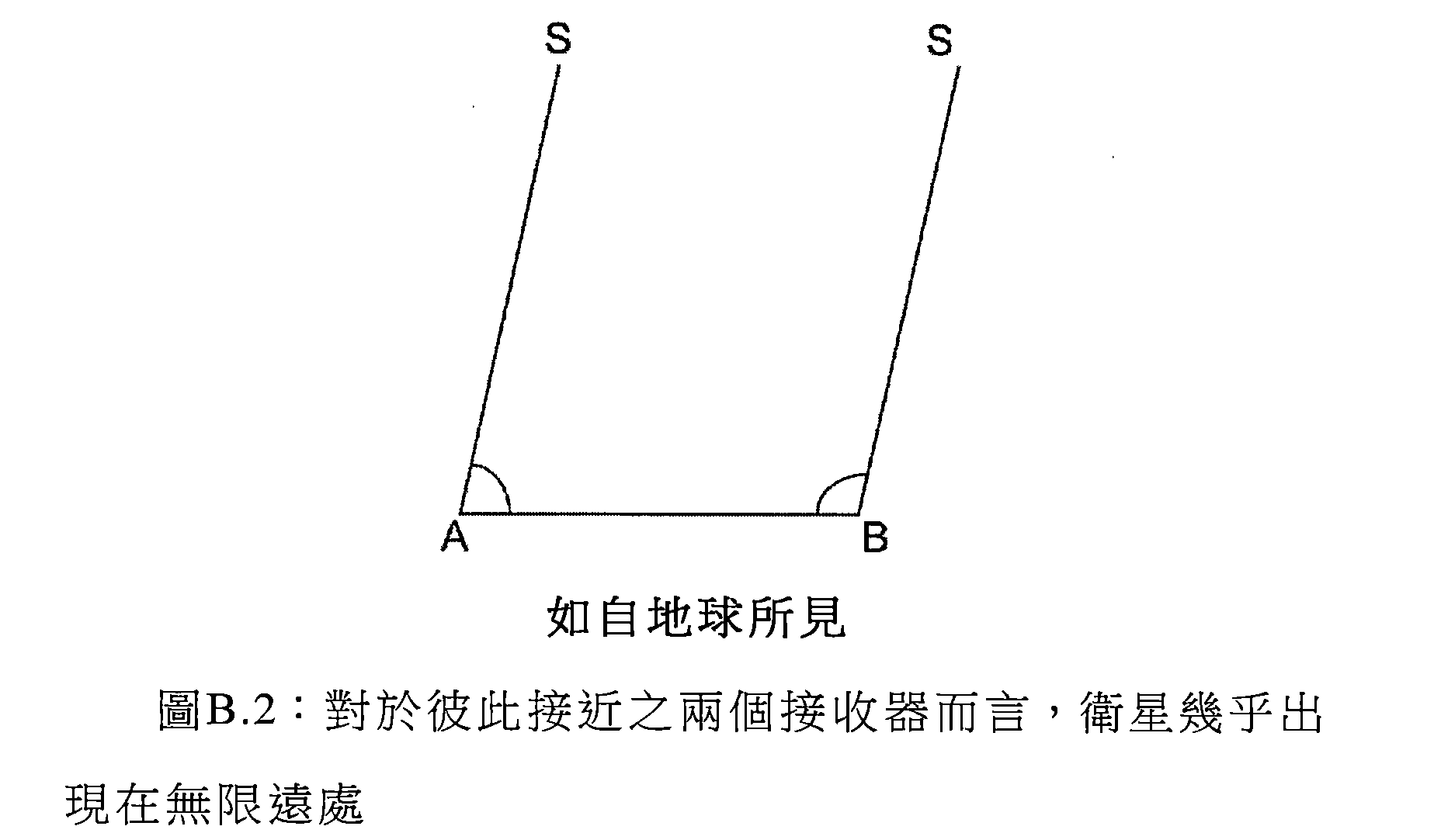
GPS衛星至少約20,000km遠,因此對於幾十公里之任何基線,此係有效的假定。 GPS satellites are at least about 20,000 km away, so this is a valid assumption for any baseline of tens of kilometers.
此意謂對於兩個接收器存在指向衛星之共同向量。吾人稱此為單位法向量

在採取方位向量(位移向量)與單位法向量之點積的情況下,吾人可將距離差項重寫如下。 In the case where the dot product of the orientation vector (displacement vector) and the unit normal vector is taken, the distance difference term can be rewritten as follows.

此允許吾人將方程式B.10重寫如下。 This allows us to rewrite equation B.10 as follows.
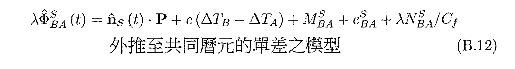
方位向量為吾人想要求解之物。方位向量告知使用者B之方位如何與使用者A相關。 The orientation vector is what we want to solve. The orientation vector informs the user how the orientation of B is related to user A.
在使用代碼可觀測量的情況下,可獲得基於自主代碼之解,其亦由接收器時脈偏差組成。然而,與基於自主代碼之解自身相比較,此等不足夠準確以允許使用方程式B.12進行方位準確度之改良。為經設計用於精確度時序應用的單頻帶接收器之Ublox LEA-6T主張「高達15ns之準確度」[15],其等於在方程式B.12中引入約4.5m之誤差。此 給予吾人用於進行雙差的動機,雙差消除進行同時觀測的接收器自身之系統誤差 In the case of code observables, a solution based on autonomous code can be obtained, which also consists of receiver clock skew. However, compared to the solution based on the autonomous code itself, these are not sufficiently accurate to allow for improved azimuth accuracy using equation B.12. The Ublox LEA-6T, designed for single-band receivers for precision timing applications, claims "accuracy up to 15 ns" [15], which is equivalent to introducing an error of approximately 4.5 m in equation B.12. this Giving us the motivation to make double difference, double difference elimination, systematic error of the receiver itself for simultaneous observation
B.2 雙差B.2 double difference
雙差為單差之差。當進行同時觀測時,雙差消除接收器自身之系統誤差。此等誤差包括接收器時脈偏差。 The double difference is the difference between the single differences. When performing simultaneous observations, the double difference eliminates the systematic error of the receiver itself. These errors include receiver clock skew.
吾人仍使用接收器A及B採取兩個衛星S2及S1之兩個單差。吾人亦需要同時採取此等單差。當GPS使用CDMA時此同時性係可能的,此意謂GPS接收器同時看到天空中之每一衛星。方程式B.13展示單差對。 We still use receivers A and B to take two single differences between the two satellites S2 and S1. We also need to take these single differences at the same time. This simultaneity is possible when GPS uses CDMA, which means that the GPS receiver sees each satellite in the sky at the same time. Equation B.13 shows a single difference pair.

在採取兩式之差的情況下,吾人得到下式,其中


相位多路徑可高達觀測的四分之一循環且並不自一個位點至另一位點很好相關[28],因此雙差中之多路徑分量可高達一個循環。雜項誤差分量取決於許多事物,但若吾人假定其僅歸因於準確量測相位之能力且吾人假定吾人可量測相位為循環之1%,則吾人將預期雜項誤差分量為循環之4%。實際上由此,多路徑可在使用雙差時為定位誤差之主要源。 Phase multipath can be as high as one quarter of the observed cycle and is not well correlated from one site to another [28], so the multipath component of the double difference can be as high as one cycle. The miscellaneous error component depends on many things, but if we assume that it is only due to the ability to accurately measure the phase and we assume that we can measure the phase to 1% of the cycle, then we will expect the miscellaneous error component to be 4% of the cycle. In fact, multipath can be the main source of positioning error when using double difference.
B.2.1雙差解譯B.2.1 double difference interpretation
△nS2S1被吾人稱為差量範數,而散佈著方位向量之任何向量被稱為方向向量。差量範數因此亦為方向向量。吾人注意到,用於雙差之方向向量不再為單位向量。此之解譯可運用以下圖來可視化。 I is referred to as △ n S2S1 difference norm, the scattered direction vectors of any vector direction vector is called. The difference norm is therefore also the direction vector. We have noticed that the direction vector used for the double difference is no longer a unit vector. This interpretation can be visualized using the following diagram.

出於簡潔起見,使

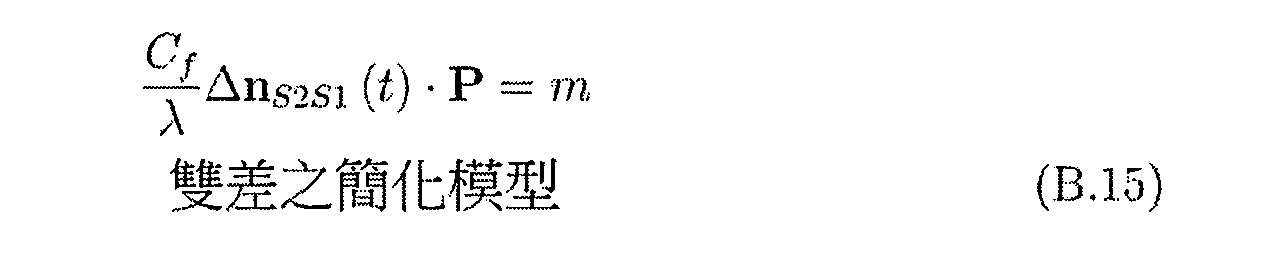
P為吾人希望求解的未知數,因此吾人將其視為變數。作為變數,存在滿足方程式B.15的P之許多值,不僅僅係吾人尋找的P=B-A,因此吾人現在可不再說P=B-A。吾人現在尋找方程式B.15之解採用的何種形式,因此得知吾
人之雙差模型的解。當吾人知曉


在重排後,吾人就看到

若吾人將P及


此意謂方程式B.14之解形成位於接收器B上之平面。吾人說此平面為雙差之解平面。 This means that the solution of equation B.14 forms a plane on receiver B. We say that this plane is the solution plane of the double difference.
B.2.2雙差循環滑移B.2.2 Double-difference cycle slip
理想地,方程式B.14中之雙差中的整數

如可看到,半循環及全循環模糊度兩者已被偵測,因此,接收器(Ublox LEA-6T)在此繪圖產生時並不使用導航資料來重新建構載波。在此狀況下,自繪圖易於看到循環滑移出現之處及校正其所需要之物,但此未必總是如此,尤其是在接收器廣泛地分離時。各種方式已經設計以偵測及/或校正雙差循環滑移。未校正及/或未偵測之循環滑移嚴重影響方位解準確度[46]。 As can be seen, both the half cycle and the full cycle ambiguity have been detected, so the receiver (Ublox LEA-6T) does not use navigation data to reconstruct the carrier when this plot is generated. In this case, self-drawing is easy to see where the loop slip occurs and what is needed to correct it, but this is not always the case, especially when the receiver is widely separated. Various approaches have been designed to detect and/or correct double-difference cycle slip. Uncorrected and/or undetected cyclic slips severely affect the accuracy of the azimuth solution [46].
B.2.3雙差殘餘B.2.3 Double difference residual
雙差殘餘(或簡言之,殘餘)為所量測之雙差與在給出方位P的情況下所預期之雙差之間的差;在循環中殘餘被書寫如下。 The double difference residual (or in short, the residual) is the difference between the measured double difference and the expected double difference in the case where the orientation P is given; the residual is written as follows in the loop.

作為獲得如何校正解或多少誤差在雙差中之想法的方式,殘餘係有用的。 The residual is useful as a way to get an idea of how to correct the solution or how much error is in the double difference.
B.3 包裝雙差B.3 Packaging double difference
吾人針對關於衛星S1及S2以及接收器A及B的雙差之正分數分量定義以下記號,並將其稱為包裝雙差,其中{}為鋸齒形函數。 We define the following notation for the positive fractional components of the double differences for satellites S1 and S2 and receivers A and B, and call them the package double difference, where {} is a zigzag function.
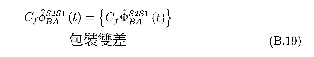
在使此與吾人之雙差模型相等的情況下,吾人看到下式。 In the case where this is equal to our double-difference model, we see the following formula.
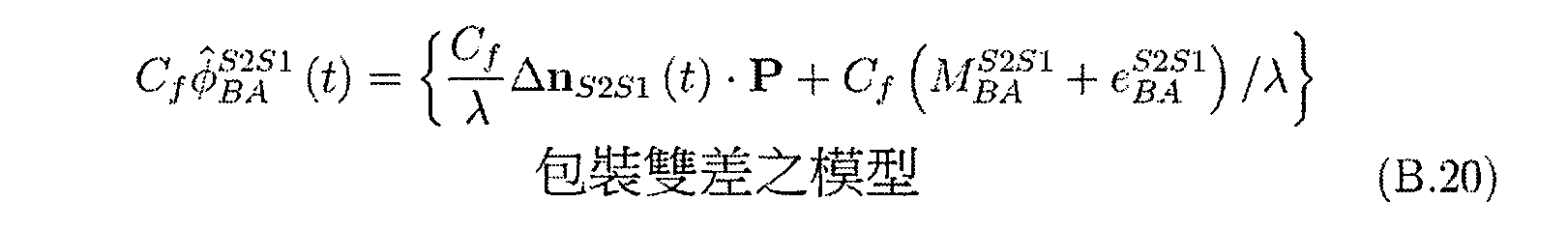
此為用於包裝雙差之吾人之模型。包裝雙差移除未知整數N,從而移除循環滑移。 This is the model used to wrap the double difference. The package double difference removes the unknown integer N, removing the loop slip.
B.3.1包裝雙差解譯B.3.1 Packaging double difference interpretation
包裝雙差藉由包裝雙差而移除未知整數N。當相對於時間標繪來自一對衛星的包裝雙差時,吾人得到看起來類似於以下圖之某圖。資料似乎被包裝,因此其得名。 The package double difference removes the unknown integer N by wrapping the double difference. When plotting the double difference of the package from a pair of satellites with respect to time, we get a picture that looks similar to the one below. The information seems to be packaged, so it gets its name.

圖B.7:使用隔開幾公分之兩個GPS接收器針對一對衛星之包裝雙差資料。 Figure B.7: Packaging double-difference data for a pair of satellites using two GPS receivers separated by a few centimeters.
圖B.7係針對相隔僅僅幾個公分置放的兩個接收器對於在大於此之距離處的接收器,當標繪包裝雙差時吾人得到的繪圖視覺上變得無意義且看起來像除了均質點塊以外什麼都沒有。 Figure B.7 is for two receivers placed just a few centimeters apart. For receivers at distances greater than this, the plots we get when plotting the double difference in the package visually become meaningless and look like There is nothing but a homogeneous block.
出於簡潔起見,使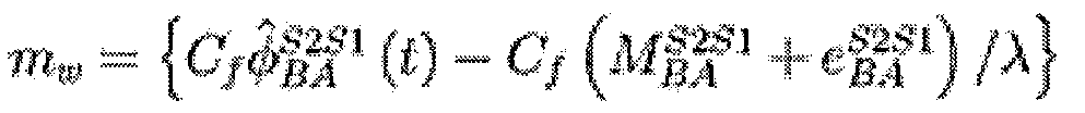

可以類似於針對子章節B.2.1中之雙差模型進行的的方式得知對於包裝雙差的吾人之模型的解之形式。吾人尋找方程式B.21之解採取的何種形式。當吾人知曉


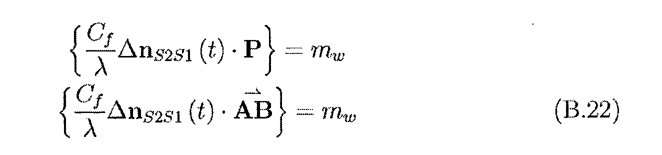
採取兩式之差。 Take the difference between the two.

此類似於針對雙差之解採取的形式,惟此次歸因於鋸齒形函數而存在無限數目個平面除外。為除移除鋸齒形函數,吾人注意到,存在k 

此意謂
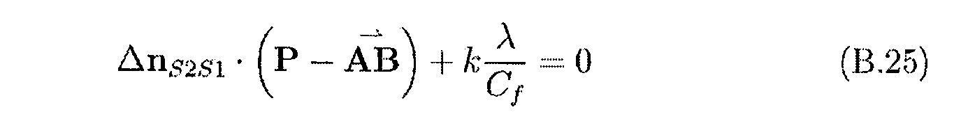
此可被重寫如下,其中μ S2S1=λ/(C f ∥△n S2S1∥)。 This can be rewritten as follows, where μ S 2 S 1 =λ/( C f ∥Δn S 2 S 1 ∥).
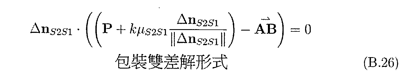
因此,解形成平面無限集。一個平面與用於雙差之解平面相同,且其他平面平行於此平面,其中每一平面彼此之間具有μ S2S1 公尺之固定間隔。因此吾人將μ S2S1 稱為平面間隔。下圖可視化無限解平面集合中之三個平面。 Therefore, the solution forms a plane infinite set. One plane is the same as the solution plane for the double difference, and the other planes are parallel to this plane, with each plane having a fixed interval of μ S2S1 meters from each other. Therefore, we call μ S2S1 a plane interval. The following image visualizes three planes in an infinite solution plane set.

B.3.2包裝相位可觀測量B.3.2 Packaging phase observable measurement
吾人將包裝相位可觀測量定義如下。 We define the phase observable measurement of the package as follows.

可將此如下使用方程式B.8外推至共同曆元t。 This can be extrapolated to the common epoch t using equation B.8 as follows.

在給出兩個接收器A及B的情況下,接著可形成單差,吾人將包裝單差稱為

且最終將兩個包裝單差給予兩個不同衛星S1及S2,可形成包裝雙差。 Finally, the two package differences are given to two different satellites S1 and S2, which can form a package double difference.

因此,在給出包裝相位可觀測量的情況下,有可能形成外推至共同曆元之包裝雙差。其以此方式進行的優點在於,與給定準確度之正常相位可觀測量相比較,需要較少位元來表示包裝相位可觀測量;此節省網路頻寬。 Therefore, given the appreciable measurement of the package phase, it is possible to form a package double difference that is extrapolated to a common epoch. The advantage of doing this in this way is that fewer bits are needed to represent the package phase observables compared to the normal phase observables of a given accuracy; this saves network bandwidth.
歸因於鋸齒形函數之屬性,當自四個包裝觀測建立包裝雙差時,僅需要一個鋸齒形操作;此可被書寫如下。 Due to the properties of the zigzag function, only one zigzag operation is required when building a package double difference from four package observations; this can be written as follows.

B.3.3解開包裝雙差B.3.3 Unpacking the double difference
解開為一種自包裝雙差重新建立雙差之方法。 Unraveling is a method of re-establishing double difference for self-packaging double difference.
首先,吾人將鋸齒形差函數定義如下。 First, we define the zigzag difference function as follows.
f(x)={x+0.5}-0.5 (B.32) f ( x )={ x +0.5}-0.5 (B.32)
此處,吾人定義進行解開並用於CFF演算法的演算法。α 

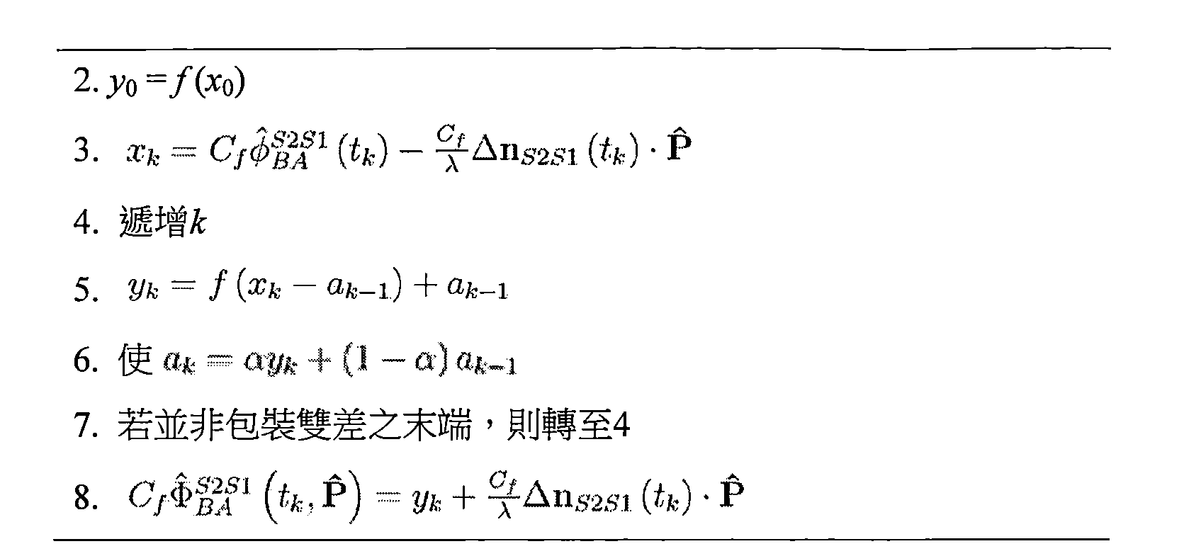
此解開演算法需要近似方位估計
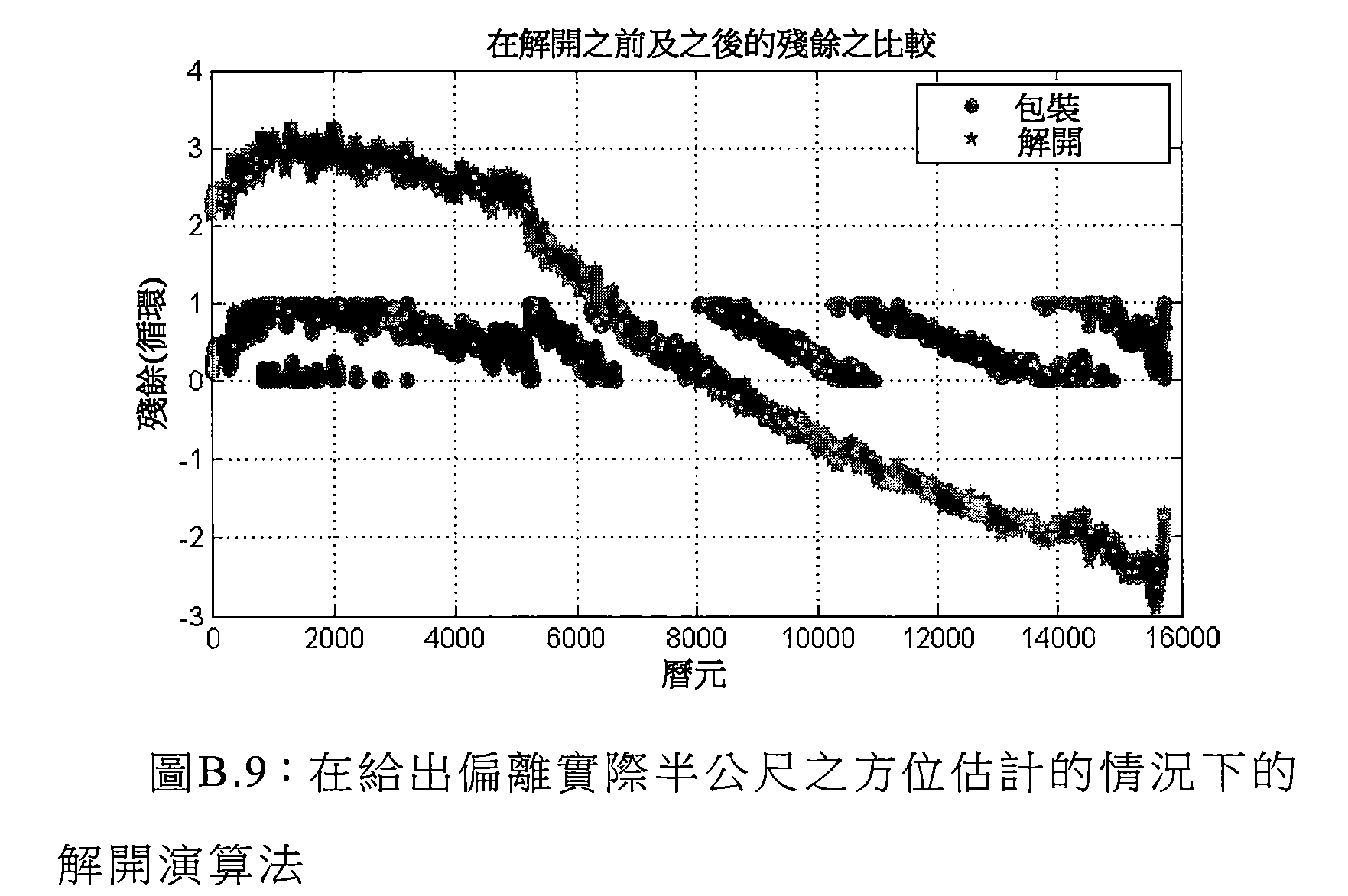
解開演算法可藉由引入循環滑移而出錯,特別是當資料為間歇(對於吾人之情境常常係此狀況)時。然而,如吾人應看到,解開演算法對於靜態情境(諸如吾人之情境)出 人意料很好地進行。 The unwrapping algorithm can make mistakes by introducing loop slips, especially when the data is intermittent (this is often the case for my situation). However, as I should see, the unwrapping algorithm is for static situations (such as my situation). The expectation is good.
B.3.4包裝雙差殘餘B.3.4 Packaging double difference residual
包裝雙差殘餘(或簡稱為包裝殘餘)為所量測的包裝或解開雙差與在給出方位P的情況下預期的雙差之間的鋸齒形差;以循環為單位,其被書寫如下。 The double residue of the package (or simply the package residue) is the zigzag difference between the measured package or the unwrapped double difference and the expected double difference given the orientation P ; in cycles, it is written as follows.
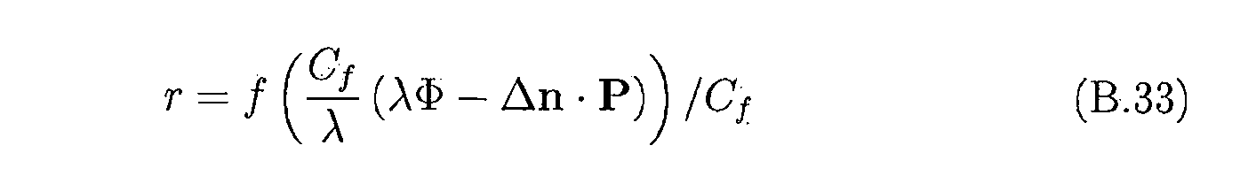
與雙差殘餘對比,包裝殘餘係循環滑移不變的。類似於雙差殘餘之包裝殘餘表達所量測物與所預期物之間的誤差。 In contrast to the double difference residual, the package residue is cyclically slippery. A package residue similar to a double difference residue expresses the error between the measured object and the expected product.
B.4 選定證明B.4 Certificate of choice
B.4.1距離變化率計算B.4.1 Distance change rate calculation
在給出
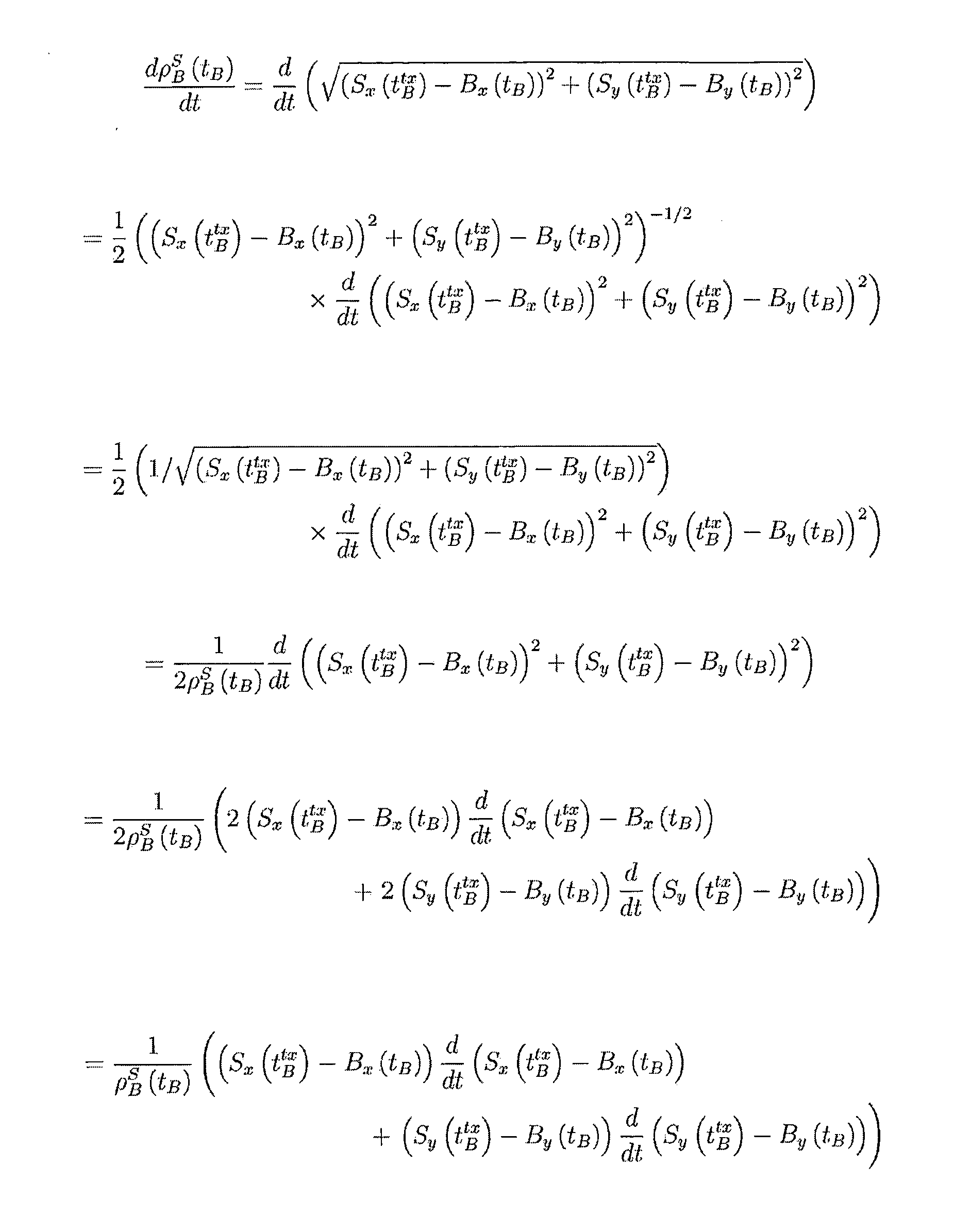

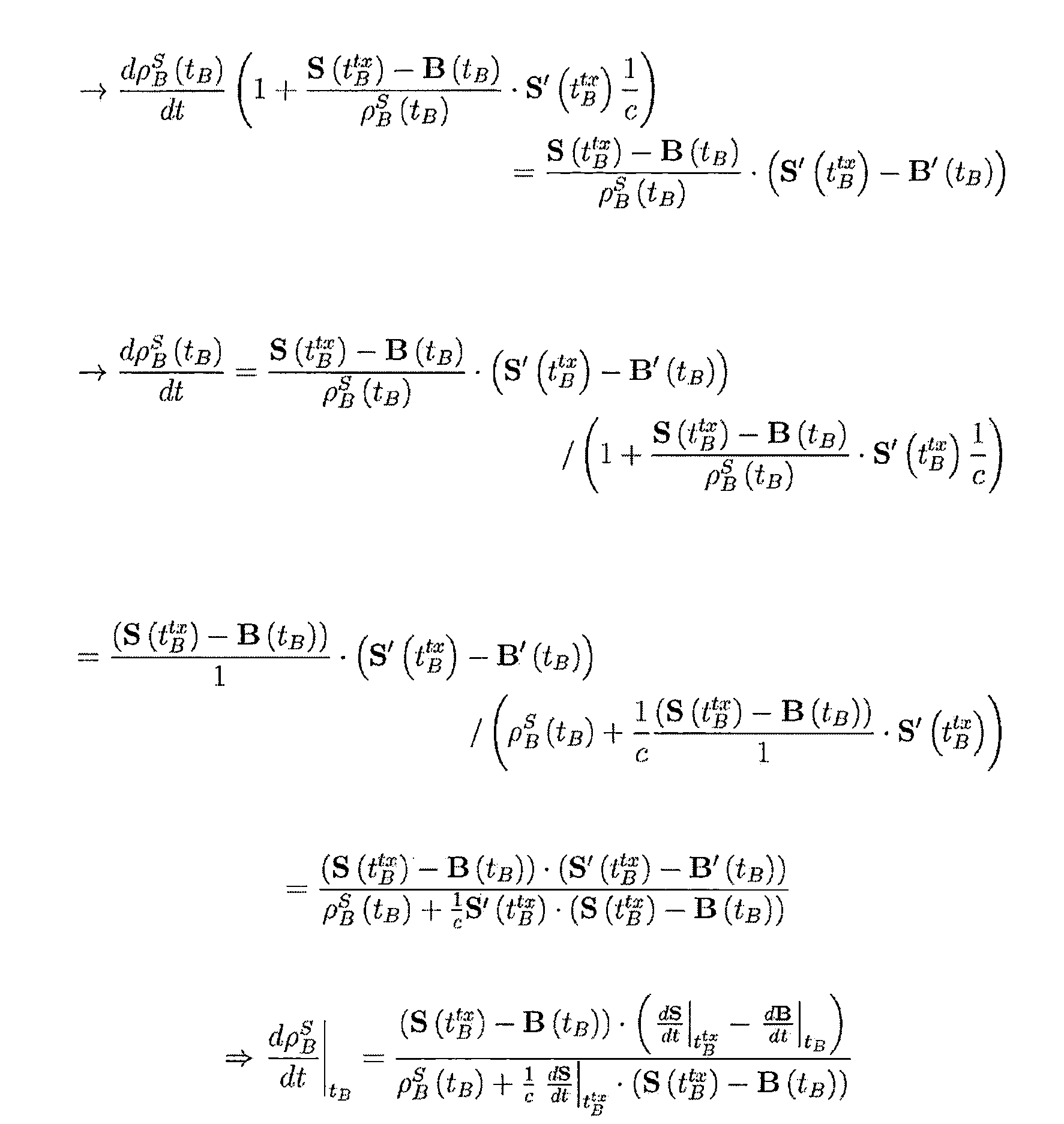
對於3D,展開式係明顯的,並得到相同公式。 For 3D, the expansion is obvious and the same formula is obtained.
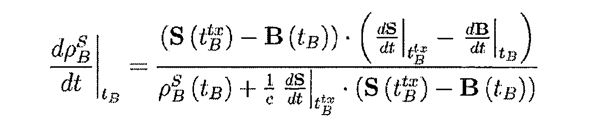
在夜晚之節點功能性Node functionality at night
作為概念證明,除了使用將時序、位置及星曆導入至GPS接收器中的輔助全球定位系統(AGPS)系統以外,吾人亦設計及實施基於晝夜節律之能量分佈演算法。33F電容器用於此測試。 As a proof of concept, in addition to the use of an auxiliary global positioning system (AGPS) system that introduces timing, position and ephemeris into a GPS receiver, we also design and implement an energy distribution algorithm based on circadian rhythm. A 33F capacitor was used for this test.
C.1 輔助GPSC.1 Assisted GPS
為了擴展在夜晚使用諸如33F電容器之極小能量儲存裝置相當均一地獲得的觀測,需要具有極低導通時間之極低工作循環([44]之第5章);此促動吾人設計AGPS系統。AGPS系統經由替代鏈路而非來自衛星之通常50波特通訊通道來將星曆、曆書及近似時間及方位供應至GPS模組。此允許GPS接收器節省不必收聽衛星的時間以恰好獲得星曆及曆書資料。 In order to extend the observations obtained fairly uniformly at night using very small energy storage devices such as 33F capacitors, an extremely low duty cycle with extremely low on-time is required (Chapter 5 of [44]); this motivates us to design an AGPS system. The AGPS system supplies ephemeris, almanac and approximate time and orientation to the GPS module via an alternate link instead of the usual 50 baud communication channel from the satellite. This allows the GPS receiver to save time when it is not necessary to listen to the satellite to get the ephemeris and almanac data.
輔助GPS之吾人之實施方案包含自由Ublox提供之Assistnow伺服器獲得星曆、曆書及近似時間。此資料保存在本地PC上並週期性地與Assistnow伺服器同步。此PC以大約250kb/s之速率在具有相異個人區域網路(PAN)識別(ID)的專用通道(AGPS通道)上使用802.15.4無線電連續地發送出此資料。具有不同PAN ID之另一通道(主通道)用於自GPS節點擷取資料並將其發送回至個人電腦(PC)。圖C.1展示此通訊實施方案。 The implementation of Assisted GPS includes the Assistnow server provided by Free Ublox to obtain ephemeris, almanac and approximate time. This data is saved on the local PC and periodically synchronized with the Assistnow server. The PC continuously transmits this data using an 802.15.4 radio at a rate of approximately 250 kb/s on a dedicated channel (AGPS channel) with distinct Personal Area Network (PAN) identification (ID). Another channel (main channel) with a different PAN ID is used to retrieve data from the GPS node and send it back to the personal computer (PC). Figure C.1 shows this communication implementation.

對於主通道,歸因於來自AGPS通道之串擾,需要確認以避免在主通道上之封包丟失。 For the primary channel, due to crosstalk from the AGPS channel, an acknowledgment is required to avoid packet loss on the primary channel.
在任何特定時間之輔助GPS資料的量並不恆定,而是約3kB量。GPS接收器可在約300ms內運用GPS資料初始化,此類似於直接自衛星下載此資料之約15分鐘。 The amount of assisted GPS data at any given time is not constant, but is about 3kB. The GPS receiver can be initialized with GPS data in about 300 ms, which is similar to the 15 minutes of downloading this material directly from the satellite.
在晴朗的天空情況下,在運用或不運用輔助GPS資料的吾人之實施方案的情況下,在沒有被供應至GPS接收器之後備功率的情況下,吾人進行10次試驗。對於每一試驗記錄TTFF且結果在下圖中標繪。 In the case of a clear sky, with the implementation of our own GPS with or without the aid of GPS data, we conducted 10 tests without being supplied to the GPS receiver. TTFF was recorded for each test and the results are plotted in the figure below.
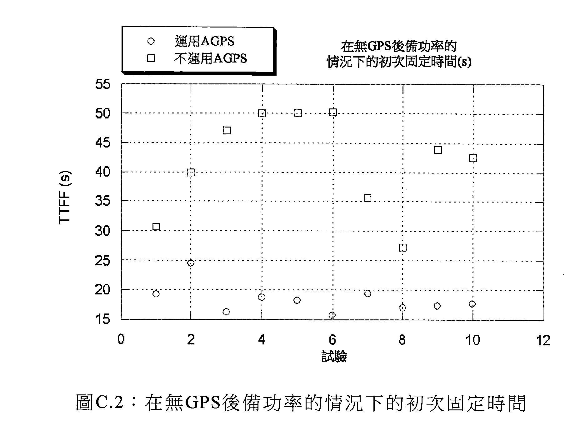
如可看到,使用AGPS系統時之TTFF顯著低於不使用AGPS系統時的TTFF。與使用AGPS系統時之18秒相比較,不使用AGPS時之平均時間為42秒。接著,根據量測使用大約30μW向GPS接收器供應後備功率的情況下,再次進行此TTFF測試;在每一試驗之間使用60秒之週期。結果在下圖中描繪。 As can be seen, the TTFF when using the AGPS system is significantly lower than the TTFF when the AGPS system is not used. The average time when AGPS is not used is 42 seconds compared to 18 seconds when using the AGPS system. Next, in the case where the backup power was supplied to the GPS receiver using approximately 30 μW according to the measurement, the TTFF test was performed again; a period of 60 seconds was used between each test. The results are depicted in the figure below.

初次GPS試驗TTFF比剩餘試驗大得多的原因係歸因於以下事實:GPS後備功率直至彼試驗才給予電力。排除初次試驗,與不使用吾人之AGPS實施方案時之10秒相比較,吾人之AGPS實施方案產生4秒之TTFF。 The reason why the initial GPS test TTFF is much larger than the remaining test is due to the fact that the GPS backup power is not supplied until the test. Excluding the initial test, our AGPS implementation produced a 4 second TTFF compared to 10 seconds when we did not use our AGPS implementation.
運用及不運用GPS後備功率的情況下,TTFF在兩種狀況下皆為大約一半。 With and without GPS backup power, TTFF is about half in both cases.
試驗之間的時間段在使用GPS後備功率時係重要的,此係因為在施加後備功率時GPS接收器保持的任何資訊將老化;在足夠長時間段情況下,其保持的任何資訊將變得無用。舉例而言,除了四個小時老化以外通常並不使用星曆。因此,當使用AGPS並供應GPS後備功率時進行30分鐘之較長間隔。採取此類型之七個依序試驗且結果在下圖中標繪。 The time period between trials is important when using GPS backup power because any information held by the GPS receiver will age when the backup power is applied; any information it maintains will become available for a sufficiently long period of time. useless. For example, ephemeris is usually not used except for four hours of aging. Therefore, a longer interval of 30 minutes is used when using AGPS and supplying GPS backup power. Seven sequential tests of this type were taken and the results were plotted in the figure below.

排除初次試驗的情況下,此測試平均TTFF為5秒。此展示高達30分鐘之節點非作用中狀態時段在使用AGPS及GPS後備功率的情況下最低限度地影響TTFF。 In the case of the initial test, the average TTFF for this test was 5 seconds. This shows that the node inactive state period of up to 30 minutes minimally affects TTFF with AGPS and GPS backup power.
在夜晚之工作循環可被計算如下
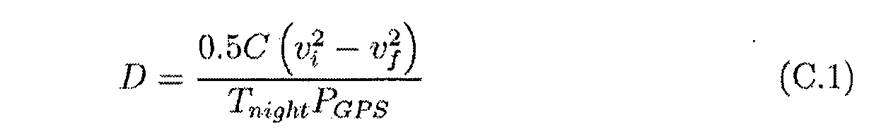
如可看到,工作循環隨夜晚長度而變。因此,假定夜晚長度為12小時,則吾人看到工作循環為大約0.5%,不必說此係極低工作循環。 As can be seen, the duty cycle varies with the length of the night. Therefore, assuming a night length of 12 hours, we see a duty cycle of about 0.5%, not to mention that this is an extremely low duty cycle.
接通時間之浪費百分比被給出如下,其中t on 為工作循環之每一作用中部分的接通時間。 The percentage of waste of the on time is given as follows, where t on is the on time of each active portion of the duty cycle.
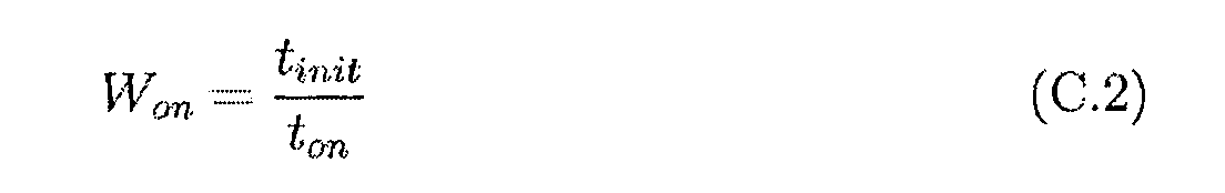
而在整個夜晚期間作用中時段之數目被給出如下。 The number of active periods during the entire night is given below.

因此,吾人採取50%之接通時間的浪費百分比,此暗示在使用吾人之AGPS給出5秒之TTFF的情況下,10秒之接通時段。此又暗示在整個夜晚期間大約20個作用中時段。每一作用中時段持續10秒,且用於此等作用中時段中之每一者的此能量的一半歸因於初始化而浪費掉。雖然工作循環為0.5%,但此百分比之一半歸因於初始化而浪費,吾人預期僅僅夜晚之0.25%獲得觀測;吾人將此稱為有效工作循環。 Therefore, we take a 50% turn-on time waste percentage, which implies a 10 second turn-on period in the case of using our AGPS to give a 5 second TTFF. This in turn implies approximately 20 active time periods throughout the night. Each active period lasts 10 seconds, and half of this energy for each of these active periods is wasted due to initialization. Although the duty cycle is 0.5%, one-half of this percentage is wasted due to initialization, and we expect only 0.25% of the night to be observed; we call this an effective work cycle.
C.2 晝夜節律能量分佈演算法C.2 Circadian rhythm energy distribution algorithm
為了在夜晚進行量測,儲存於電容器上之能量必須在整個夜晚期間被分佈以進行此任務。除此之外,亦必須在整個夜晚期間有足夠能量保留以運行類似於微處理器之其他此等事物。為了允許此發生,吾人設計及實施基於晝夜節律之想法的能量分佈演算法。以下描述該演算法。 In order to measure at night, the energy stored on the capacitor must be distributed throughout the night to perform this task. In addition to this, there must be enough energy to remain throughout the night to run other things like microprocessors. To allow this to happen, we design and implement an energy distribution algorithm based on the idea of circadian rhythm. The algorithm is described below.
第一假定為始終可在一天的白天時間期間對電容器充滿電。若並非如此,則吾人說電容器對於太陽能面板太大或太陽能面板不夠大。必須對於每一太陽能面板及電容器組合檢查此假定。 The first assumption is that the capacitor can be fully charged during the daylight hours of the day. If this is not the case, then we say that the capacitor is too large for the solar panel or the solar panel is not large enough. This assumption must be checked for each solar panel and capacitor combination.
第二假定為用以獲得觀測之全部時間段花費相同時間段及能量。此等時間段中之每一者稱為事件。 The second assumption is that it takes the same time period and energy to obtain the entire time period of the observation. Each of these time periods is called an event.
存在兩個事件類型,觸發及隔開。 There are two event types, triggered and separated.
觸發事件可在任何時間發生。當電容器之電壓超過2.2V之固定電壓時其發生。 Trigger events can occur at any time. It occurs when the voltage of the capacitor exceeds a fixed voltage of 2.2V.
另一類型之事件為隔開事件。此等事件如下圖中所描繪在最後觸發事件與第一觸發事件之間均勻隔開發生。 Another type of event is to separate events. These events occur as evenly spaced between the last trigger event and the first trigger event as depicted in the following figure.

在隔開事件階段期間最後觸發事件與第一觸發事件之間的隔開事件之能量的總和大約等於電容器之可用能量。 The sum of the energies of the spaced events between the last trigger event and the first trigger event during the interval event phase is approximately equal to the available energy of the capacitor.
在最後觸發事件之後的α/(n+1)發生第一隔開事件,且大約每隔α/(n+1)發生直至第一觸發事件。n為充滿電之電容器在未變平的情況下及在未得到任何新能量輸入的情況下可進行事件的次數,而α為在隔開事件階段期間最後觸發事件與第一觸發事件之間的時間段。 [Alpha] after the last trigger event / (n +1) spaced apart from the occurrence of a first event and a first trigger event occurs until approximately every α / (n +1). n is the number of times the fully charged capacitor can be evented without being flattened and without any new energy input, and α is between the last trigger event and the first trigger event during the interval event phase period.
當節點開始進行隔開事件時,其將直至隔開事件中之至少第三事件出現才進行觸發事件。在隔開事件階段期間監測電壓不足且若遇到則將停止進行隔開事件。若電壓仍高於固定電壓(比如2.2V),則事件將延長。每當隔開事件發生時就更新事件之間隔。隔開事件之數目係藉由考量在事件之後的當前電容器電壓、每一隔開事件使用的能量之量及下一觸發事件可能要多久而計算。節點使即時日歷時脈(RTCC)一直保持作用中。RTCC並不在全球設定任何特定時間,其僅僅大約每隔24小時循環。其沒有必要知曉具體時間是什麼,但其有必要對地球繞其自身軸旋轉花費多久有想法。其進行與吾人之晝夜節律相同的功能。 When a node begins a separation event, it will not trigger until the third event in the interval event occurs. The monitoring voltage is insufficient during the interval event phase and the separation event will be stopped if encountered. If the voltage is still higher than a fixed voltage (such as 2.2V), the event will be extended. The interval of events is updated whenever a separate event occurs. The number of spaced events is calculated by considering the current capacitor voltage after the event, the amount of energy used by each spaced event, and how likely the next trigger event may be. The node keeps the Instant Calendar Clock (RTCC) active. RTCCs are not set globally for any given time, they only cycle around every 24 hours. It is not necessary to know what the specific time is, but it is necessary to have an idea of how long it takes for the Earth to rotate around its own axis. It performs the same function as our circadian rhythm.
C.3 晝夜節律能量分佈演算法及AGPS系統實施結果C.3 Circadian rhythm energy distribution algorithm and AGPS system implementation results
接著,晝夜節律能量分佈演算法連同如所描述之AGPS系統一起實施於硬體上並被測試。以下描述自此系統獲得之結果。 Next, the circadian energy distribution algorithm is implemented on the hardware along with the AGPS system as described and tested. The results obtained from this system are described below.
在下午5:00,節點持續大約18小時置放在外部且記錄節點之超級電容器電壓;圖C.6展示此等量測之結果;如可看到,此圖表看起來類似於圖C.5中之圖表。 At 5:00 pm, the node is placed externally for approximately 18 hours and the node's supercapacitor voltage is recorded; Figure C.6 shows the results of these measurements; as can be seen, this chart looks similar to Figure C.5 Chart in the middle.
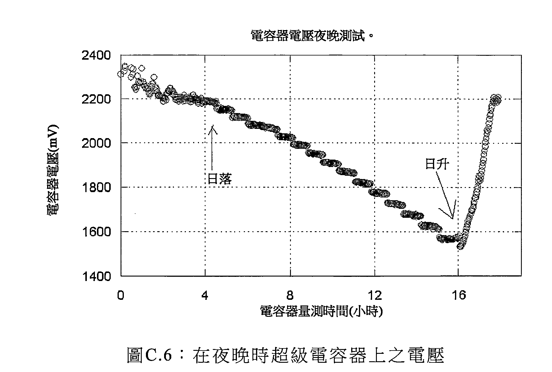
在圖C.6中可看到的在整個夜晚期間之短尖銳下降係由GPS進入作用中並採取量測所造成。在整個夜晚期間僅僅存在大約14個量測,而非較接近於如在最後觸發事件與第一觸發事件之間的整個時段期間所預期的20個量測的原因係因為節點晝夜節律直至完整24小時過去才同步。 The short sharp drop during the entire night that can be seen in Figure C.6 is caused by the GPS entering the action and taking measurements. There are only about 14 measurements during the entire night, rather than being closer to the 20 measurements expected during the entire time period between the last trigger event and the first trigger event because the node circadian rhythm is up to 24 It’s only after the hour has passed.
持續大約75小時進行測試,記錄GPS模組之基於自主代碼之方位解,計算此資料集合之平均值且接著對於每一方位解,自此平均值之偏移被計算並標繪於圖C.7中。 The test is continued for approximately 75 hours, the azimuth solution of the GPS module based on the autonomous code is recorded, the average of the data set is calculated, and then for each azimuth solution, the offset from this average is calculated and plotted in Figure C. 7 in.
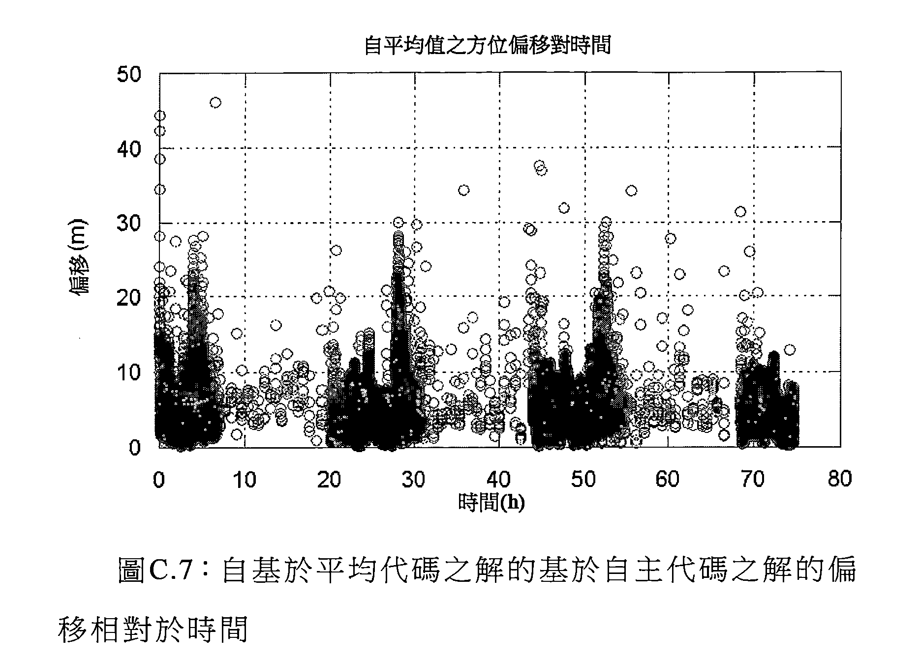
圖C.7中之較低密度地方係在夜晚獲得之方位解,高密度地方係日間解。對於此測試,一個標準差等於2.9m。對於每一隔開事件計算大約7.7個方位解。在一年的特定時間在彼位置處,夜間大約持續13小時,此意謂在夜晚一秒0.003方位解之解密度,或0.3%之有效工作循環;此非常好地與0.25%之近似預期有效工作循環相比較。 The lower density areas in Figure C.7 are the azimuth solutions obtained at night, and the high density areas are daytime solutions. For this test, one standard deviation is equal to 2.9m. Approximately 7.7 azimuthal solutions are calculated for each spaced event. At a specific time of the year at the position, the night lasts for approximately 13 hours, which means a solution density of 0.003 azimuth solution at one second in the night, or an effective duty cycle of 0.3%; this is very good with an approximate expected effect of 0.25%. Work cycle comparison.
在白天期間,實際上吾人藉由比較可說工作循環為100%,因此解之99.7%係在白天期間獲得。然而,夜間時之資料在整個夜晚期間相對均勻地隔開,此係能量分佈之目標。因此,吾人之能量分佈演算法有效於在夜晚操作GPS接收器,使得不極大地叢集其得到之觀測。在夜晚獲得觀測之可能優點可能係作為減輕解偏差之方式。另外,GPS接收器能夠有時在夜晚操作並在夜晚之彼等時間內至少獲 得基於自主代碼之解,從而增加時間資訊。 During the day, in fact, by comparison, we can say that the work cycle is 100%, so 99.7% of the solution is obtained during the day. However, the data at night is relatively evenly spaced throughout the night, which is the target of energy distribution. Therefore, our energy distribution algorithm is effective in operating GPS receivers at night so that the observations obtained therefrom are not greatly clustered. The possible advantages of obtaining observations at night may be a way to mitigate the bias. In addition, GPS receivers can sometimes operate at night and receive at least during the night. Based on the solution of the autonomous code, it adds time information.
歸因於時間約束、增加之複雜度及吾人主要關注通常來自24小時時段之許多觀測形成一個解的靜態解,因此並未進一步採取在整個夜晚期間分佈觀測。然而,吾人已展示實際上有可能在夜晚使用極低工作循環及或非常大電容器獲得解。顯然,許多其他新演算法可以較大複雜度建立以允許諸如恆星濾波及獲得基於曆元之解之此等技術。 Due to time constraints, increased complexity, and our main focus on many observations, usually from a 24-hour period, form a static solution to the solution, so no further observations are made throughout the night. However, we have shown that it is actually possible to obtain solutions at night using very low duty cycles and very large capacitors. Obviously, many other new algorithms can be built with greater complexity to allow such techniques as stellar filtering and obtaining epoch-based solutions.
網路network
資料必須在節點與進行最終處理之主電腦之間傳送。吾人將此分成兩個區段;WSN區段及網際網路區段。網際網路區段由在已進行任何處理之後自其到達基地台之時起的資料流程組成,處理係諸如時間模糊度解析、重複封包移除、非依序封包移除等等。WSN區段由資料流程及節點之經處理資料之間的處理(直至其交遞至網際網路區段)組成。 The data must be transferred between the node and the host computer for final processing. We divide this into two segments; the WSN segment and the Internet segment. The Internet segment consists of a data flow from the time it arrives at the base station after any processing has been performed, such as temporal ambiguity resolution, repeated packet removal, non-sequential packet removal, and the like. The WSN segment consists of processing between the data flow and the processed data of the node (until it is handed over to the Internet segment).
D.1 網際網路區段D.1 Internet segment
網路之網際網路結構為直播器、伺服器、用戶端結構。此為網際網路協定RTCM網路連接輸送(NTRIP)用於在網際網路上存取GPS接收器的相同想法。實施自訂直播器、伺服器、用戶端結構之吾人自身的實施方案,吾人稱其為JAC封包。下圖展示用於兩個試驗台之結構。 The network structure of the network is a live broadcaster, a server, and a client-side structure. This is the same idea that the Internet Protocol RTCM Network Connection Transport (NTRIP) is used to access GPS receivers over the Internet. Implementing the implementation scheme of the custom broadcaster, server, and client structure, we call it JAC packet. The figure below shows the structure used for two test stands.

裝置伺服器充當用於WSN閘道器裝置及實體連接之GPS接收器兩者的驅動器以及資料至JAC封包直播器之供應器。因而,其任務中之一些任務係用於網際網路區段,而其他任務係用於WSN區段。在先前圖中,裝置伺服器上之虛線表示其兩個任務之間的接面。裝置伺服器充當JAC封包直播器可連接至以獲得希望記錄在JAC封包伺服器處之資料的伺服器。JAC封包直播器經由保持開啟的TCP連接而附接至JAC封包伺服器,且JAC封包伺服器記錄來自每一試驗台之傳入資料。JAC封包用戶端接著可連接至JAC封包伺服器且獲得來自試驗台之經記錄資料或來自試驗台 中之一者的即時串流。對於連接至JAC封包伺服器之JAC封包直播器,鑑認係經由使用者名稱及密碼;對於JAC封包用戶端不實施鑑認要求。不對基地台進行資料之記錄,意謂若網際網路連接停止,則資料將丟失。 The device server acts as a driver for both the WSN gateway device and the physically connected GPS receiver and as a provider of data to the JAC packet live broadcaster. Thus, some of its tasks are for the Internet segment and other tasks are for the WSN segment. In the previous figures, the dashed line on the device server indicates the junction between its two tasks. The device server acts as a JAC packet live broadcaster that can be connected to a server that obtains the data that is desired to be recorded at the JAC packet server. The JAC packet live broadcaster is attached to the JAC packet server via a TCP connection that remains open, and the JAC packet server logs incoming data from each test station. The JAC packet client can then connect to the JAC packet server and obtain recorded data from the test bench or from the test bed. Instant streaming of one of the ones. For the JAC packet live broadcaster connected to the JAC packet server, the authentication is via the user name and password; for the JAC packet client, the authentication requirement is not implemented. Failure to record data on the base station means that if the Internet connection is stopped, the data will be lost.
D.2 WSN區段D.2 WSN section
在設計階段期間,因為與建立困難多跳網路相比較,獲得解之處理程序更重要,所以最初設想單跳網路。然而,在臺灣廬山之真實壽命試驗台中,節點傳輸距離被發現為並不足夠且需要延伸距離之方式。歸因於節點上之有限時間及有限資源兩者,設計及實施專用中繼器節點以延伸距離。 During the design phase, the single-hop network was originally conceived because it was more important to obtain a solution to the solution than to establish a difficult multi-hop network. However, in the real life test bench of Laoshan, Taiwan, the node transmission distance was found to be insufficient and the way to extend the distance. Due to the limited time and limited resources on the node, a dedicated repeater node is designed and implemented to extend the distance.
以下圖像展示節點、中繼器及基地台之專用於建立經交遞至網際網路區段之資料的部分。 The following image shows the nodes, repeaters, and base stations dedicated to establishing the material that is handed over to the Internet segment.

D.2.1 中繼器D.2.1 Repeater
為了使用中繼器,將兩個額外位元組添加至每一資料封包。一個位元組為序號,而另一位元組為8個旗標,其中 每一旗標對應於中繼器節點編號之模8。資料封包序號不與每一802.15,4封包之標頭中的序號相同。 In order to use the repeater, two extra bytes are added to each data packet. One byte is a sequence number, and another tuple is 8 flags, of which Each flag corresponds to the modulo 8 of the repeater node number. The data packet sequence number is not the same as the sequence number in the header of each 802.15, 4 packet.
每當封包由節點傳輸時資料封包序號就將增加。同時所傳輸之旗標位元組將被設定為零。因此,收聽資料封包之任何人將能夠告知此等封包之次序,使其中之任一者遺漏,外加知曉其來自節點而非中繼器,此係因為旗標位元組已被設定為零。 The data packet sequence number will increase each time the packet is transmitted by the node. At the same time, the transmitted flag byte will be set to zero. Therefore, anyone listening to the data packet will be able to inform the order of these packets, leaving any of them missing, plus knowing that they are from the node instead of the repeater, since the flag byte has been set to zero.
中繼器含有其最近藉由儲存802.15.4標頭封包序號及源節點編號而發送之小封包清單。當中繼器聽到封包時,若中繼器發現其已發送該封包,則其將不再次發送該封包;此有助於防止無限傳輸循環發生及重複中繼器已發送的資料。另外,當中繼器聽到封包時,若中繼器發現中繼器旗標位元組之其位元已經被設定,則其將不再次發送此封包;雖然可能並不嚴格地需要,但此完全防止無限傳輸循環發生。 The repeater contains a list of small packets that it recently sent by storing the 802.15.4 header packet sequence number and the source node number. When the repeater hears the packet, if the repeater finds that it has sent the packet, it will not send the packet again; this helps prevent the infinite transmission loop from occurring and repeating the data that the repeater has sent. In addition, when the repeater hears the packet, if the repeater finds that its bit of the repeater flag byte has been set, it will not send the packet again; although it may not be strictly required, this is completely Prevent infinite transmission loops from occurring.
當中繼器發送封包時其欺騙802.15.4標頭以便匹配於發端節點。此欺騙資訊意謂802.15.4標頭中之源MAC位址及序號兩者匹配於發端節點之源MAC位址及序號。中繼器設定對應於中繼器之節點編號的中繼器旗標位元組之位元。另外,中繼器使用節點編號及802.15,4標頭封包序號更新經傳輸封包清單。使用802.15.4標頭封包序號而非資料封包序號的原因係允許節點有機會發送複本封包以縮減封包丟失。 When the repeater sends a packet, it spoofs the 802.15.4 header to match the originating node. The spoofing information means that the source MAC address and the sequence number in the 802.15.4 header match the source MAC address and sequence number of the originating node. The repeater sets the bit of the repeater flag byte corresponding to the node number of the repeater. In addition, the repeater updates the list of transmitted packets using the node number and the 802.15, 4 header packet sequence number. The reason for using the 802.15.4 header packet sequence number instead of the data packet sequence number is to allow the node to have the opportunity to send a replica packet to reduce packet loss.
吾人意識到,歸因於聽到來自一節點之同一封包而兩 個中繼器同時傳輸的可能性仍繼續存在。然而,若中繼器可彼此聽到,則csma/ca演算法應至少設法減輕此效應,使得來自中繼器之兩個所得封包被依序發送。 I realized that due to hearing the same packet from one node, two The possibility of simultaneous transmission of repeaters continues. However, if the repeaters can hear each other, the csma/ca algorithm should at least try to mitigate this effect so that the two resulting packets from the repeater are sent sequentially.
D.2.2 裝置伺服器D.2.2 device server
裝置伺服器之作用的另一半係自其聽到之「節點演算法資料」求解時間模糊度、移除複本封包,及移除非依序封包。 The other half of the role of the device server is to solve the temporal ambiguity, remove the duplicate packet, and remove the non-sequential packet from the "node algorithm data" that it hears.
首先,裝置伺服器求解時間模糊度。為了移除複本封包及非依序封包,裝置伺服器進行以下操作。其追蹤循環緩衝器中之自每一節點接收之最後10個唯一資料封包。若在循環緩衝器中找到封包,則其被視為複本且被丟棄。若其並非為複本,則封包被放入循環緩衝器中。若封包之GPS時間比循環緩衝器中之其他10個封包中之任一者早,則封包被丟棄。否則,其經傳遞至網際網路區段。此防止複本封包及封包之非依序次序兩者傳遞至網際網路區段。 First, the device server solves the time ambiguity. In order to remove the duplicate packet and the non-sequential packet, the device server performs the following operations. It tracks the last 10 unique data packets received from each node in the circular buffer. If a packet is found in the circular buffer, it is considered a duplicate and discarded. If it is not a duplicate, the packet is placed in a circular buffer. If the GPS time of the packet is earlier than any of the other 10 packets in the circular buffer, the packet is discarded. Otherwise, it is passed to the Internet segment. This prevents both the duplicate packets and the non-sequential order of the packets from being passed to the Internet segment.
D.2.3 相控D.2.3 Phase control
中繼器僅僅重複其聽到的封包;其不知曉封包將何時到達。由此,對於充當中繼器之中繼器,其無線電必須連續地接通,此使用使GPS接收器接通使用的功率之大約70%。此為相當大的功率,意謂需要工作循環。 The repeater simply repeats the packets it hears; it does not know when the packet will arrive. Thus, for a repeater acting as a repeater, its radio must be continuously turned on, this use causes the GPS receiver to turn on approximately 70% of the power used. This is a considerable amount of power, meaning that a work cycle is required.
雖然可能不存在足夠輻照度以使任一節點連續地保持作用中,但若節點全部輪流在作用中,則有可能存在一個節點在白天時間期間始終在作用中,因此強迫中繼器連續地接通。當然,若不存在足夠輻照度,則一個中繼器不可 連續地在作用中狀態中。若節點及中繼器在某種程度上全部經同步以變得同時在作用中且節點及中繼器兩者大約獲得相同量的輻照度,則節點接著在中繼器必須在非作用中之前將全部變得在非作用中,此係因為與中繼器相比較,節點在某種程度上使用更多功率;因此中繼器將完全地伺服節點需要。 Although there may not be enough irradiance to keep any node in active, if all the nodes are active, there may be a node that is always active during daylight hours, thus forcing the repeater to continuously connect through. Of course, if there is not enough irradiance, then one repeater is not available. Continuously in the active state. If the node and the repeater are all synchronized to some extent to become active at the same time and both the node and the repeater obtain approximately the same amount of irradiance, then the node then before the repeater must be inactive All become inactive, because the node uses more power to some extent because it is compared to the repeater; therefore the repeater will be completely needed by the servo node.
當中繼器在作用中且全部節點在非作用中時,會出現另一問題。在此狀況下,當節點最終變得在作用中時中繼器可必須變得在非作用中以節省能量,不能充當用於作用中節點之中繼器。因此,當節點活動停止時中繼器變得在非作用中係有意義的。 Another problem arises when the repeater is active and all nodes are inactive. In this case, the repeater may have to become inactive to save energy when the node eventually becomes active, and cannot act as a repeater for the active node. Therefore, when the node activity stops, the repeater becomes meaningful in the inactive.
自此等兩個問題,形成對WSN網路中之全部節點及中繼器進行相控的想法。該想法係使中繼器及節點同時變得在作用中且同時變得在非作用中;以便彼此同相。 From these two issues, the idea of phase control of all nodes and repeaters in the WSN network is formed. The idea is to make the repeater and the node become active at the same time and at the same time become inactive; so as to be in phase with each other.
因為雙差可僅由來自同時接通之兩個GPS接收器之觀測形成,所以對同時變得在作用中之節點進行相控意謂,與節點彼此不同相的情況相比較,可由節點自身形成更多雙差。雖然觀測引起關注,但歸因於時間約束,並不研究此效應。 Since the double difference can be formed only by observations from two GPS receivers that are simultaneously turned on, phase control of the nodes that are simultaneously in effect means that the nodes themselves can be formed as compared with the case where the nodes are out of phase with each other. More double difference. Although observations are of concern, they are not studied due to time constraints.
D.2.3.1 相控演算法D.2.3.1 Phased algorithm
吾人設計及實施針對吾人之節點及中繼器的相控演算法。此演算法之主要假定係全部節點及中繼器獲得相同輻照度。 We design and implement phased algorithms for our nodes and repeaters. The main assumption of this algorithm is that all nodes and repeaters get the same irradiance.
在假定輻照度對於全部節點及中繼器相同的情況下, 全部節點可具有相同工作循環及接通時間,在中繼器相比於節點在作用中時使用稍微較少的功率的相同時間,中繼器可至少匹配於節點之工作循環及接通時間。 Under the assumption that the irradiance is the same for all nodes and repeaters, All nodes may have the same duty cycle and turn-on time, and the repeater may match at least the duty cycle and turn-on time of the node at the same time that the repeater uses slightly less power than when the node is active.
無論節點是否正獲得適用之觀測,節點皆將發送資料封包以向節點及中繼器兩者通知節點使其GPS接收器接通;當不可獲得適用之觀測時此等封包將為空白,否則其將含有通常「節點演算法資料」。若其為空白,則其在裝置伺服器處被丟棄。 Regardless of whether the node is getting the applicable observations, the node will send a data packet to inform both the node and the repeater that the node is connected to its GPS receiver; these packets will be blank when no applicable observations are available, otherwise Will contain the usual "node algorithm data". If it is blank, it is discarded at the device server.
當節點之超級電容器達到2.2V時,其被視為充滿且節點將開始相控時段,若未聽到GPS封包,則相控時段將在10分鐘之後逾時。在下圖中描繪如在節點上所運行的相控演算法。 When the supercapacitor of the node reaches 2.2V, it is considered full and the node will start the phase control period. If the GPS packet is not heard, the phase control period will expire after 10 minutes. The phased algorithm as run on the node is depicted in the following figure.

在吾人之實施方案中,在節點相控期間需要相對小功率,此係因為使用大約10mW或GPS接收器在接通的情況下將使用的功率之4%,節點僅僅持續2秒接通其無線電且接著再次持續18秒關斷。在吾人之實施方案中,此相控時段可持續高達10分鐘。在此相控時段期間若聽到表示其他節點使其GPS接收器接通的任何資料封包,則節點將退出 相控時段並開始正常收集觀測的GPS資料。另一方面,若在10分鐘之後仍沒有聽到表示其他節點使其GPS接收器接通之資料封包,則節點將退出相控時段並開始正常收集觀測的GPS資料。 In our implementation, relatively low power is required during node phase control, because the node uses only about 10 mW or 4% of the power that the GPS receiver will use when it is turned on, the node only turns on its radio for 2 seconds. And then continue for another 18 seconds to turn off. In our implementation, this phase control period can last up to 10 minutes. If any data packet indicating that other nodes have their GPS receiver connected is heard during this phase control period, the node will exit The phased time period and the normal collection of observed GPS data began. On the other hand, if after 10 minutes, the data packet indicating that the other node has its GPS receiver turned on is not heard, the node will exit the phase control period and start to collect the observed GPS data normally.
在下圖中描繪如在中繼器上所運行的相控演算法。 The phased algorithm as run on the repeater is depicted in the following figure.
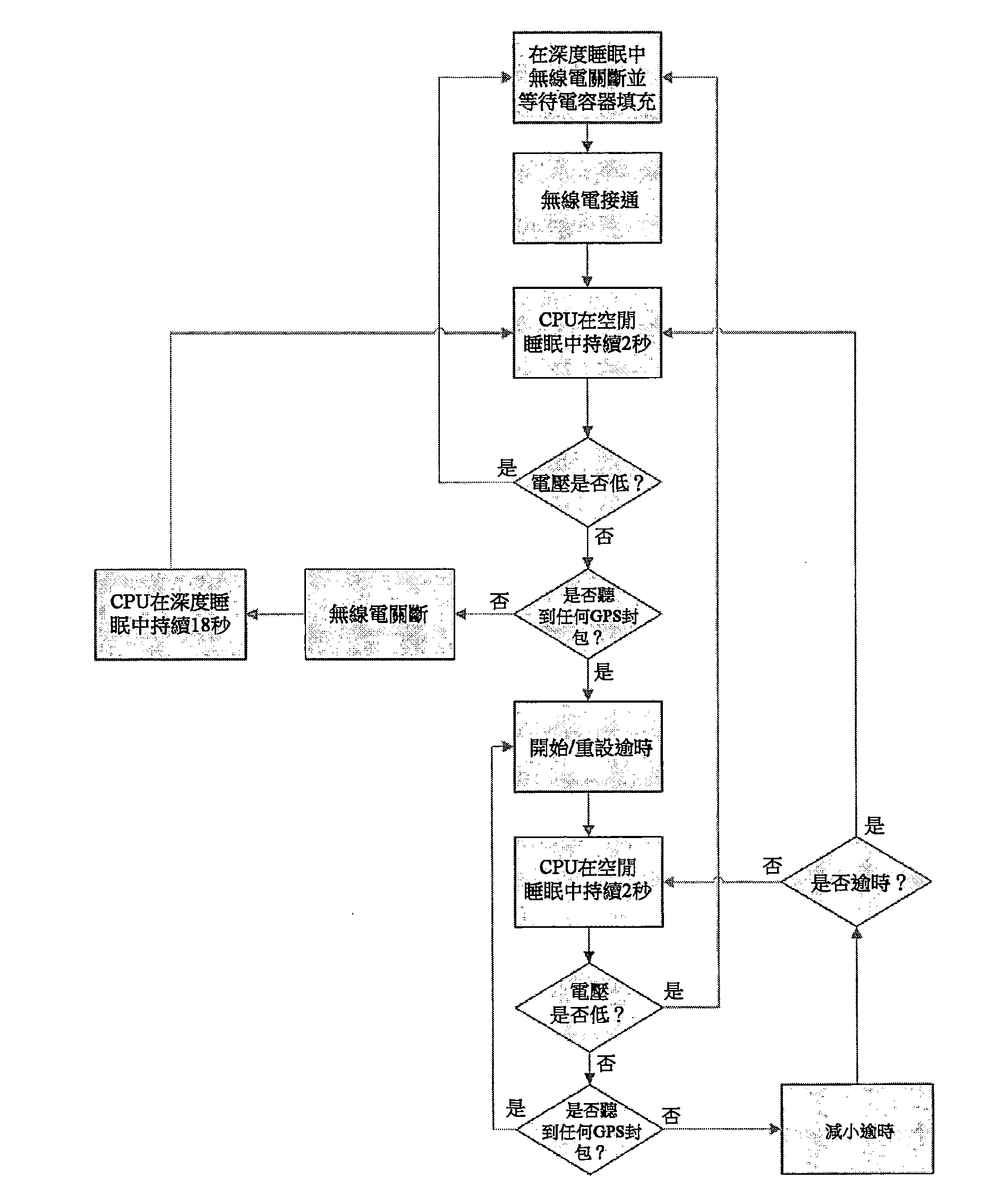
在無節點活動之時間期間,中繼器運行相控時段,中繼器將持續2秒接通其無線電以收聽資料封包且接著再次關斷。若聽到表示其他節點使其GPS接收器接通之資料封包,則中繼器接著變得在作用中,且若未聽到表示其他節點使其GPS接收器接通之新資料封包,則將被觸發的逾時開始。當逾時被觸發時中繼器再次返回至相控時段中。只要中繼器在其演算法中,若電容器之電壓位準變得太低,則無線電就將關斷且中繼器將等待其超級電容器電壓再次上升至2.2V。 During the time of no-node activity, the repeater runs a phased period, and the repeater will turn its radio on for 2 seconds to listen to the data packet and then turn it off again. If a packet of data indicating that the other node has its GPS receiver turned on is heard, the repeater then becomes active and will be triggered if a new data packet indicating that the other node has its GPS receiver turned on is not heard. The timeout begins. When the timeout is triggered, the repeater returns to the phase control period again. As long as the repeater is in its algorithm, if the voltage level of the capacitor becomes too low, the radio will turn off and the repeater will wait for its supercapacitor voltage to rise again to 2.2V.
多路徑及恆星濾波Multipath and stellar filtering
基於曆元之解為此時使用來自一個曆元之觀測來獲得解的解。基於每天之解為此時使用來自一天之全部可用觀測來獲得解的解。在此論文中吾人主要集中於基於每天靜態之解。 The solution based on the epoch is to use the observation from one epoch to obtain the solution of the solution at this time. Based on the daily solution, the solution is obtained using all available observations from one day at this time. In this paper, we mainly focus on solutions based on static everyday.
演算法之恆星部分使用固定解及相對於有偏位置的絕對包裝殘餘堆疊兩者之堆疊技術實施恆星濾波;此經設計以改良在觀測為間歇的吾人之特定情境下之解準確度及精確度。在此章中,吾人藉由研究被證明係吾人之雙差中的最大誤差源的多路徑而開始。自此,假定模糊度解析度為求解問題,吾人重寫吾人之雙差模型以包括僅僅多路徑及加成性白高斯雜訊並判定當間歇地採取觀測時吾人獲得的吾人之解的分佈。吾人接著導出吾人之恆星濾波公式並展示在模擬中及在真實壽命中其實際上改良吾人之解。吾人亦展示歸因於吾人獲得觀測之隨機間歇性質,與吾人使用連續供電GPS接收器輸出恆定高速率觀測相比較,吾人在解精確度方面獲得較大改良。 The stellar portion of the algorithm implements stellar filtering using a stacking technique of both fixed solutions and absolute package residual stacks with biased positions; this is designed to improve the accuracy and precision of the solution in the specific context of the observations that are intermittent. . In this chapter, we begin by studying the multipath of the largest source of error in the double difference that proves to be ours. From then on, assuming that the ambiguity resolution is a solution problem, we rewrite our double-difference model to include only multipath and additive white Gaussian noise and to determine the distribution of our solution obtained when we take observations intermittently. We then derive our stellar filter formula and show that it actually improves our solution in the simulation and in real life. We also show that due to the random intermittent nature of our observations, we have made significant improvements in accuracy compared to the continuous high-rate observations of continuously powered GPS receivers.
相位可觀測量之多路徑誤差歸因於經由不同路徑到達接收器之載波的疊加。此具有似乎延遲到達接收器之載波的效應。對於除了直視線信號以外的單一反射信號,相位可觀測量之多路徑誤差可經模型化如下,其中α為阻尼因數,λ為標稱波長,且Φ為兩個信號之間的循環之相位差[60]。 The phase observable multipath error is due to the superposition of carriers arriving at the receiver via different paths. This has the effect of appearing to delay the arrival of the carrier of the receiver. For a single reflected signal other than a direct line of sight signal, the multipath error of the phase observable can be modeled as follows, where α is the damping factor, λ is the nominal wavelength, and Φ is the phase difference between the two signals [ 60].

當阻尼因數等於1時此產生絕對最大誤差
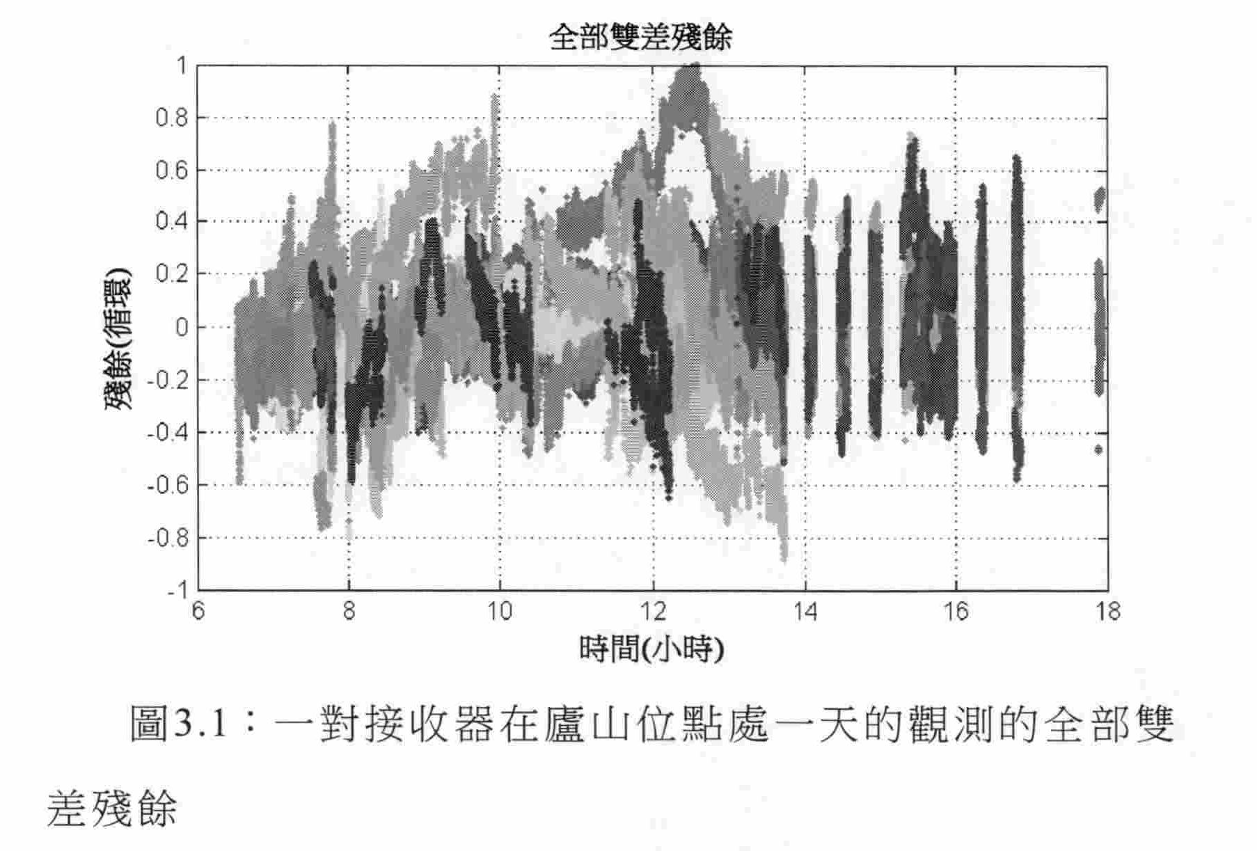
PCV似乎非常類似於多路徑,惟對天線旋轉之相依性除外。因為此情形,吾人將PCV與多路徑誤差集總在一起。如自圖3.1可看到,存在為吾人將自多路徑誤差預期的最大值之高達約一個循環之偏差。然而,解開演算法可失效且引入循環滑移,循環滑移亦可為先前圖(圖3.1)中獲得之極 高讀數中之一些的原因。在處理吾人之資料時,吾人使用為2之代碼因數,因此圖3.1中之循環滑移將引起0.5循環之偏移。吾人應看到,多路徑被證明係雙差殘餘的方差之最主要分量。此亦藉由參考文獻支援,諸如主張「多路徑為差分載波相位及虛擬距離量測中之主要誤差源」的[55]及說明「多路徑常常視為精確GPS定位中之最多限制因數」的[45]。來自圖3.1之雙差並非為用以獲得解的誤差源。實際上,使用具有最高仰角之衛星作為參考衛星的雙差之獨立集被使用;此等雙差之殘餘可在圖3.2中看到。 PCV seems to be very similar to multipath, except for the dependence on antenna rotation. Because of this situation, we aggregate the PCV with the multipath error. As can be seen from Figure 3.1, there is a deviation of up to about one cycle that we would expect from the multipath error. However, the unwrapping algorithm can fail and introduce cyclic slip, which can also be obtained from the previous graph (Figure 3.1). The reason for some of the high readings. When dealing with our data, we use a code factor of 2, so the cyclic slip in Figure 3.1 will cause a 0.5 cycle offset. We should see that multipath is proved to be the most important component of the variance of the double difference residual. This is also supported by references such as "Multipath is the main source of error in differential carrier phase and virtual distance measurement" [55] and "Multipath is often considered the most limiting factor in accurate GPS positioning". [45]. The double difference from Figure 3.1 is not intended to be used as a source of error for the solution. In fact, an independent set of double differences using the satellite with the highest elevation angle as the reference satellite is used; the residual of these double differences can be seen in Figure 3.2.
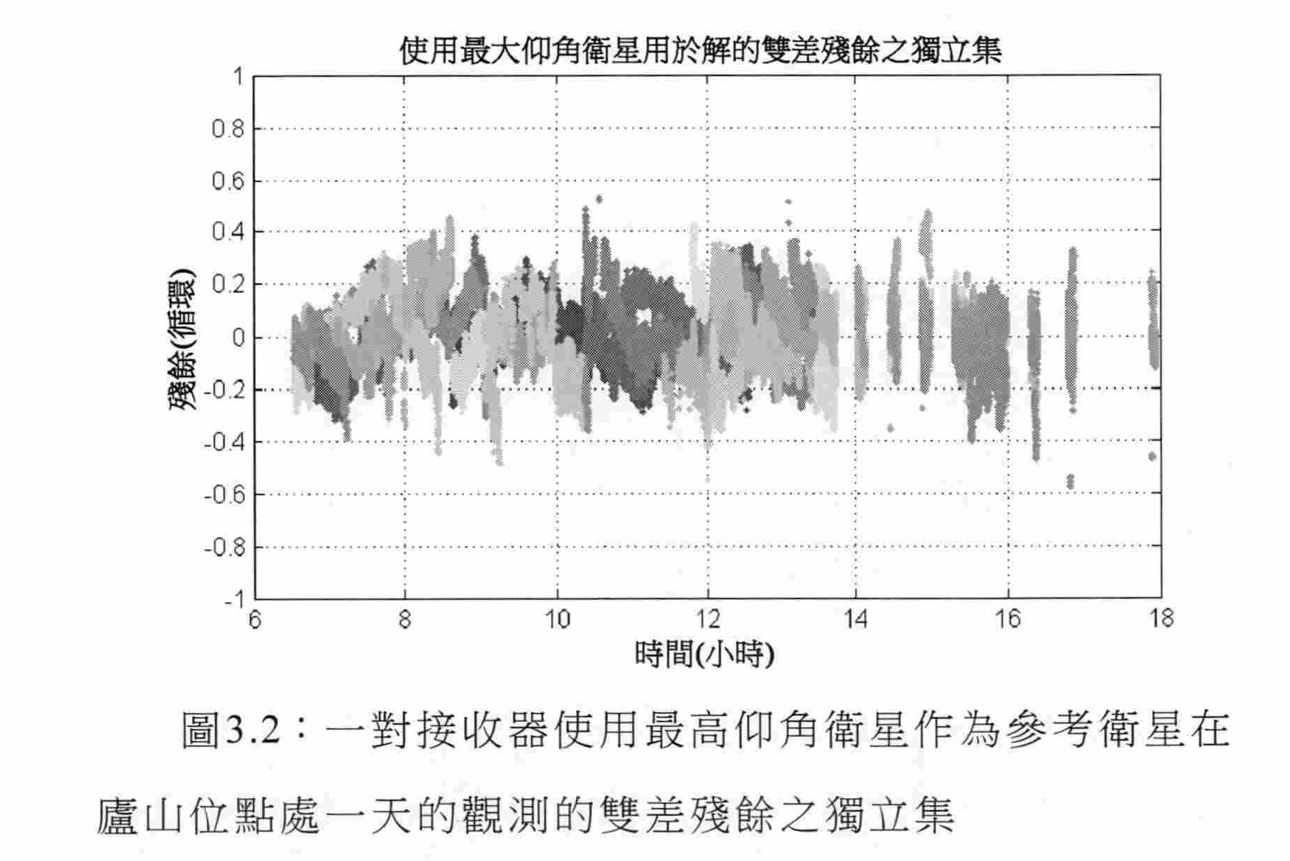
自圖3.2,顯而易見的是,方差顯著較少,但如吾人應看到仍比平均量測雜訊大很多。 From Figure 3.2, it is obvious that the variance is significantly less, but as I should see it is still much larger than the average measurement noise.
自圖3.1中之殘餘,出現在幾個小時之相對長時間內緩慢變化的大分量。除了緩慢分量以外,出現週期性且具有通常約5至10分鐘之時段的快速分量亦可看到且在某種程 度上具有三角形性質。若吾人僅少量放大來自圖之跡線中的一者,則快速週期性分量可更清晰地看到;此可在圖3.3中看到。 The remnants from Figure 3.1 appear as large components that change slowly over a relatively long period of several hours. In addition to the slow component, a fast component that appears periodic and has a period of typically about 5 to 10 minutes can also be seen and in some way Degree has a triangular nature. If we only zoom in on one of the traces from the graph, the fast periodic component can be seen more clearly; this can be seen in Figure 3.3.

此高度時間相關多路徑被稱為鏡面多路徑且由光滑表面(可能是地面)之反射產生且當每一曆元計算解時及亦如在吾人之當針對一整天計算一個解時的狀況下導致定位誤差[41,20]。在高多路徑環境中,解誤差可為實質性且為約幾個公分[20]。 This height-time-dependent multipath is called specular multipath and is generated by the reflection of a smooth surface (possibly the ground) and when each epoch calculates a solution and also as when we calculate a solution for a whole day The resulting positioning error [41, 20]. In a high multipath environment, the solution error can be substantial and is about a few centimeters [20].
3.1 衛星及多路徑週期性3.1 Satellite and multipath periodicity
歸因於GPS衛星軌道週期,衛星大約每隔24小時246秒重複其相對於基於地面之使用者的位置,亦錯誤地被稱作GPS恆星週期(錯誤地,如恆星日並非為24小時246秒而實際上為24小時236秒)。雖然衛星具有稍微小於12小時之軌道週期,但歸因於地球之旋轉,衛星相對於基於地球之觀測者大約每隔24小時而非12小時大約出現在天空中之同一地方。GPS衛星偶爾地進行操縱以確保其大約維持相對於地球之固定地面軌跡。根據文獻,地球扁率引起升交點向 西偏移,此藉由將GPS軌道週期減小大約四秒而補償[19]。一日中存在兩個軌道週期,此引起與恆星日之大約八秒差。此值僅僅為近似值且衛星重複時間已看到變化至少9秒[24]。因為衛星重複週期僅僅為近似值,所以吾人僅使用24小時246秒之一個固定重複時間,藉由[24]之一組觀測發現該固定重複時間與平均重複時間有1秒差且匹配於資料集中藉由[34]給出的平均重複週期。在吾人之論述中,吾人將24小時246秒之GPS衛星重複時間錯誤地稱為恆星週期且將其假定為指代吾人之給定標稱衛星重複週期且並非實際恆星日長度,吾人這樣做係因為此濾波處理程序通常稱為恆星濾波而非GPS軌道重複週期濾波。 Due to the GPS satellite orbital period, the satellite repeats its position relative to the ground-based user approximately every 24 hours and 246 seconds, also incorrectly referred to as the GPS star cycle (incorrectly, if the stellar day is not 24 hours and 246 seconds) It is actually 24 hours and 236 seconds). Although the satellite has an orbital period of slightly less than 12 hours, due to the rotation of the Earth, the satellite appears approximately in the same place in the sky approximately every 24 hours instead of 12 hours relative to the Earth-based observer. GPS satellites are occasionally manipulated to ensure that they maintain a fixed ground trajectory relative to the Earth. According to the literature, the earth's flattening rate causes the ascending point to West offset, which is compensated by reducing the GPS orbit period by approximately four seconds [19]. There are two orbital periods in a day, which causes about eight seconds difference from the stellar day. This value is only an approximation and the satellite repetition time has seen a change of at least 9 seconds [24]. Since the satellite repetition period is only an approximation, we only use a fixed repetition time of 24 hours and 246 seconds. The observation of one of [24] shows that the fixed repetition time has a difference of 1 second from the average repetition time and matches the data set. The average repetition period given by [34]. In our discussion, we have incorrectly referred to the 24-hour 246-second GPS satellite repetition time as the stellar period and assumed it to refer to the given nominal satellite repetition period of ours and not the actual stellar day length. Because this filtering process is often referred to as stellar filtering rather than GPS track repetition period filtering.
多路徑隨GPS接收器之周圍環境及衛星幾何形狀而變。因此,只要GPS接收器之周圍環境不相對於GPS接收器改變,則多路徑誤差應自一個恆星日至下一恆星日係類似的。此允許判定吾人在圖3.1中看到的大誤差係歸因於多路徑抑或某一其他誤差形式的方式。在以下兩個圖3.4及圖3.5中,吾人繪製自吾人之硬體獲得的對於固定GPS接收器針對兩個相異恆星日之一對衛星的雙差殘餘;一者針對衛星對在一日中可見的整個時間,且另一者針對其之小特寫部分。 Multipath varies with the surrounding environment of the GPS receiver and the geometry of the satellite. Therefore, as long as the surrounding environment of the GPS receiver does not change relative to the GPS receiver, the multipath error should be similar from one stellar day to the next stellar day. This allows to determine the way in which the large error seen in Figure 3.1 is due to multipath or some other form of error. In the following two figures 3.4 and 3.5, we draw the double-difference residuals obtained from our hardware for a fixed GPS receiver for one of two distinct celestial days; one for satellite pairs visible in a day The whole time, and the other is aimed at its small close-up.

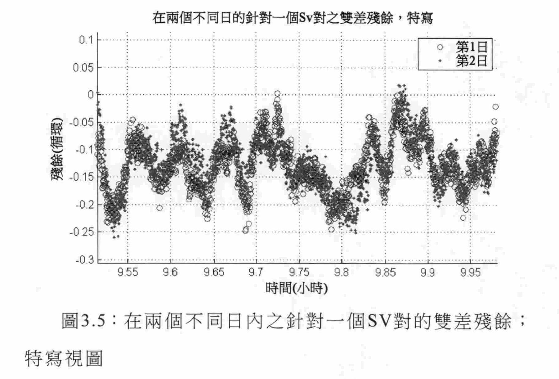
如可看到,甚至對於小快速週期性三角形分量在日之間存在非常接近匹配。因此,吾人推斷圖3.1中可見的誤差之大部分係歸因於多路徑及PCV。 As can be seen, there is a very close match between the days even for small fast periodic triangular components. Therefore, I have inferred that most of the errors seen in Figure 3.1 are due to multipath and PCV.
3.2 剩餘誤差3.2 Residual error
假定整數模糊度解析已成功,吾人可更簡單重寫吾人之雙差模型如下,其中全部下標、上標及索引已被移除。 Assuming that the integer ambiguity resolution has been successful, we can more easily rewrite our double-difference model as follows, in which all subscripts, superscripts, and indexes have been removed.
λΦ=△n.P+M+e (3.1) λΦ=△n. P+ M + e (3.1)
吾人已將剩餘誤差分成由歸因於吾人視為多路徑之幾何形狀(衛星位置、接收器周圍環境及PCV)之誤差組成的M,及雜項誤差e。雜項誤差將由量測雜訊及其他誤差組成。因為吾人僅僅使用雙差之獨立集(其中具有最大仰角之衛星用作參考衛星以用於解),所以吾人僅僅關注僅僅此等獨立雙差值中之剩餘誤差而非其他。如圖3.2中所見,吾人關注雙差而非其他者。當估計剩餘誤差時,吾人僅僅使用此等雙差。 We have divided the residual error into M consisting of errors due to the geometry (satellite position, receiver surroundings, and PCV) that we consider to be multipath, and miscellaneous error e . Miscellaneous errors will consist of measuring noise and other errors. Since we only use an independent set of double differences (where the satellite with the largest elevation angle is used as a reference satellite for the solution), we only focus on the residual error in only these independent double differences and not others. As seen in Figure 3.2, we focus on double differences rather than others. When estimating the residual error, we only use these double differences.
3.2.1量測雜訊3.2.1 Measuring noise
為了獲得量測雜訊之近似值,在給定準確方位估計情況下,對於60對衛星,吾人採取一秒時間差分雙差殘餘(r(t)-r(t-1)),接著量測平均方差。因為衛星看起來相對緩慢自地球束縛觀測者移動並假定其他誤差相對緩慢改變,所以一秒差將主要由量測雜訊組成。下圖3.6展示用於該等衛星對中之一者的用以獲得估計的一秒時間差分雙差殘餘。 In order to obtain an approximation of the measured noise, for a given pair of satellites, we take a one-second time difference double residual ( r (t)- r ( t -1)) for the 60 pairs of satellites, and then measure the average variance. Because the satellite appears to be moving relatively slowly from the Earth-bound observer and assumes that other errors change relatively slowly, the one-second difference will consist primarily of measurement noise. Figure 3.6 below shows one of these satellite pairs used to obtain an estimated one second time differential double residual.

因為此為加成性白高斯雜訊之差,所以對於雙差,此需要除以2的平方根。自此,吾人獲得歸因於0.013循環之量測雜訊的雙差之平均標準差或var(雜訊)=0.000169循環2的方差。因為量測誤差取決於信號強度,所以低至0.009循環之誤差經獲得用於一對衛星而0.019循環之最大值經獲得用於另一對衛星。因為雙差由誤差之兩個倍增組成,所以為了獲得吾人之GPS接收器中的一者的量測誤差之估計,此等值必須除以4之平方根。因此,平均起來,吾人之GPS接收器應具有95%可信度,與真值之0.013循環或約1%循環相比較,其將更好地正確地量測相位可觀測量。 Since this is the difference between additive white Gaussian noise, this is required to divide by the square root of 2 for double difference. Since then, we have obtained the mean standard deviation of the double difference or the variance of var (noise) = 0.000169 cycle 2 due to the measurement noise of 0.013 cycles. Since the measurement error is dependent on the signal strength, an error as low as 0.009 cycles is obtained for a pair of satellites and a maximum of 0.019 cycles is obtained for another pair of satellites. Since the double difference consists of two doublings of the error, in order to obtain an estimate of the measurement error of one of our GPS receivers, this value must be divided by the square root of 4. Therefore, on average, our GPS receiver should have 95% confidence that it will better measure phase observables better than a true value of 0.013 cycles or about 1% cycle.
3.2.2 多路徑誤差3.2.2 Multipath error
多路徑誤差高度取決於位置,因此,對於其方差,可能無法獲得確切值。如吾人已看到的上限針對雙差為一個循環且針對一個接收器自身為四分之一循環。另外,自實 際資料量測多路徑亦可能係複雜的,此係因為雙差殘餘之恆星差分化自一日至下一日未完全消除多路徑。此係因為雙差需要兩個衛星且因為此等兩個衛星之重複時間將不相同,嚴格地講,不存在衛星相對於彼此將在確切相同位置中的確切時間。其他人已意識到相同問題且已設計將雙差變換成單差且接著將每一衛星與更多確切重複時間對準接著將此等單差變換回成雙差的技術[62]。然而,吾人不使用此方法且超出此論文之範疇;因此吾人進行衛星之對準自一個標稱衛星重複週期至下一週期係確切相同的近似。藉由使用恆星差分化之此近似,吾人可獲得多路徑誤差及其他誤差之量值的近似想法,吾人不可運用恆星濾波之吾人特定方法來校正多路徑誤差及其他誤差。 The multipath error is highly dependent on position, so the exact value may not be obtained for its variance. As I have seen, the upper limit is one cycle for double difference and one quarter cycle for one receiver itself. In addition, self-real Inter-data measurement multipath may also be complex, because the star difference of the double-difference residual does not completely eliminate multipath from day to day. This is because two satellites are required for double difference and because the repetition times of these two satellites will be different, strictly speaking, there is no exact time when the satellites will be in exactly the same position relative to each other. Others have recognized the same problem and have designed a technique to transform the double difference into a single difference and then align each satellite with more exact repetition times and then transform these single differences back into double differences [62]. However, we do not use this method and are beyond the scope of this paper; therefore, we align the satellites from one nominal satellite repetition period to the next cycle with the exact same approximation. By using this approximation of stellar differentiation, we can obtain an approximate idea of the magnitude of multipath errors and other errors. We cannot use the specific method of stellar filtering to correct multipath errors and other errors.
圖3.7展示連續兩日之恆星差以及兩日殘餘· Figure 3.7 shows the star difference and two days of remnants for two consecutive days.

在廬山試驗台位點處在一日內對用於最終每天解之全 部衛星對進行此恆星差分計算的情況下,恆星方差之平均值經判定為0.0014,而第二日之平均值為0.0096。恆星方差可書寫為var(恆星差)=2×var(雜訊)+2×var(其他) In the case where the stellar difference calculation is performed for all satellite pairs used for the final daily solution at the site of the Laoshan test bed within one day, the average of the stellar variance is judged to be 0.0014, and the average of the second day is 0.0096. The stellar variance can be written as var (stellar difference) = 2 × var (noise) + 2 × var (other)
而第2日之方差可書寫為var(第2日)=var(雜訊)+var(其他)+var(吾人可校正之多路徑) The variance of the 2nd day can be written as var (2nd day) = var (noise) + var (other) + var (multipath that we can correct)
此又暗示

因此var(吾人可校正之多路徑)=0.0089循環 2且var(其他)=0.000531循環 2。 So var (multiple path that we can correct) = 0.0085 loop 2 and var (other) = 0.000531 loop 2 .
在進行衛星之對準自一個標稱衛星重複週期至下一週期係確切相同的近似的情況下,吾人說對於所使用之兩個接收器,在廬山試驗台處信號中之平均多路徑具有0.094循環之標準差,而其他誤差之值具有0.023循環標準差。 In the case where the satellite alignment is exactly the same approximation from one nominal satellite repetition period to the next cycle, we say that for the two receivers used, the average multipath in the signal at the Laoshan test bench has 0.094. The standard deviation of the cycle, while the value of the other error has a standard deviation of 0.023 cycles.
因此,多路徑的0.094循環之標準差對於此特定例項為下限,而1循環為上限。因此,看起來量測雜訊小於多路徑誤差至少一數量級,因此相當微不足道。其他誤差無庸置疑具有多路徑之某一分量但難以判定。吾人將其他誤差與 量測雜訊組合,吾人將其他誤差與量測雜訊稱為雜項誤差,而吾人可校正的多路徑誤差之組合,吾人稱為多路徑誤差。因此,在此特定境況中吾人獲得此等兩個誤差之以下標準差。 Therefore, the standard deviation of the 0.094 cycle of the multipath is the lower limit for this particular example, and the 1 cycle is the upper limit. Therefore, it seems that the measurement noise is at least an order of magnitude smaller than the multipath error and is therefore quite insignificant. Other errors are undoubtedly having a certain component of multipath but difficult to determine. We will have other errors Measuring the noise combination, we call other errors and measurement noises as miscellaneous errors, and the combination of multipath errors that we can correct is called multipath error. Therefore, in this particular situation, we obtain the following standard deviations of these two errors.
σ e =0.026循環 σ e =0.026 cycle
σ M =0.094循環 σ M = 0.094 cycle
定性標準差值 Qualitative standard deviation
雖然當然此取決於GPS接收器周圍環境,但其給出多路徑誤差及非多路徑誤差兩者的量值之想法。多路徑誤差此處為下限,因此係保守的。即使如此,吾人已檢查的誤差(吾人將其一起集總至多路徑中)之重複性質仍大於組合之暫時誤差的剩餘者之重複性質許多倍。因此,恆星濾波之某一形式似乎有利於使用。 Although this of course depends on the surroundings of the GPS receiver, it gives the idea of the magnitude of both multipath and non-multipath errors. The multipath error is here the lower limit and is therefore conservative. Even so, the repeating nature of the errors we have examined (which we aggregate together into the multipath) is still many times greater than the repeating nature of the remainder of the combined temporary errors. Therefore, some form of stellar filtering seems to be beneficial for use.
3.3 日間恆星濾波3.3 Daytime star filtering
日間恆星濾波解(日間解)為使用除了在自身所討論之日中可用的全部觀測以外亦使用在其他日中全部可用觀測的每天解;其他日可未必係連續日。 The daytime star filtering solution (daytime solution) uses daily solutions for all available observations in other days, in addition to all observations available on the day in which it is discussed; other days may not be consecutive days.
衛星重複性質允許吾人將在不同恆星日獲得的雙差視為好像其幾乎相同。當衛星位置相同時,若接收器位置及其周圍環境兩者皆不變,則差量範數及多路徑M亦相同。在此狀況下,若今天用以獲得方位解之雙差亦與明天用以獲得解之雙差相同,則兩個解應非常類似。 The satellite repeating nature allows us to treat the double difference obtained on different star days as if it were almost identical. When the satellite positions are the same, if the receiver position and its surroundings are unchanged, the difference norm and multipath M are also the same. Under this circumstance, if the double difference used today to obtain the azimuth solution is the same as the double difference used to obtain the solution tomorrow, the two solutions should be very similar.
吾人定義下標k及n以表示恆星日。出於簡單起見,吾人不給出表示一日內之時間的記號。對於彼此匹配的兩個 雙差,吾人定義其必須在不同恆星日相對於a p 之整數倍數分離不大於一秒,且雙差屬於同一衛星及接收器對,其中a p 為標稱GPS衛星軌道重複週期。當雙差彼此匹配時,吾人進行衛星幾何形狀對於兩個雙差係確切相同的近似。吾人將N定義為含有用於一日之每一可能差量範數,而N k 含有僅僅在第k日使用的差量範數,類似記號用於多路徑,M用於在一日期間之每一可能的多路徑,且M k 用於在第k日使用的多路徑。 We define subscripts k and n to represent stellar days. For the sake of simplicity, we do not give a sign indicating the time of day. For two double differences that match each other, we define that they must be separated by no more than one second from an integer multiple of a p on different star days, and the double difference belongs to the same satellite and receiver pair, where a p is the nominal GPS satellite orbit Repeat cycle. When the double differences match each other, we make the satellite satellite geometry exactly the same approximation for the two double difference systems. We define N as containing each possible difference norm for one day, while N k contains the difference norm used only on the kth day, similar tokens are used for multipath, and M is used during one day. Every possible multipath, and Mk is used for multipath used on day k .
吾人可對於一日之全部雙差及對於第k日取樣之雙差兩者之多路徑進行分解因數;亦即M=NP M +M MNL 及M k =N k P M,k +M MNL,k 。此允許吾人將方程式3.1重寫如下,此意謂吾人之解歸因於多路徑而有偏。 We can decompose the multipath of all the double differences of one day and the double difference of the sampling of the kth day; that is, M = NP M + M MNL and M k = N k P M, k + M MNL, k . This allows us to rewrite Equation 3.1 as follows, which means that our solution is biased due to multipath.
λΦ k =△n k .(P k +P M,k )+M MNL,k +e k (3.2) λΦ k =Δn k . (P k +P M,k )+ M MNL,k + e k (3.2)
因此,吾人可說對於第k日,解採取如下分佈,假定多路徑係以零平均值正態分佈,其中α k 為用於第k日之每天雙差之百分比。 Therefore, we can say that for the kth day, the solution takes the following distribution, assuming that the multipath is normally distributed with a zero mean, where α k is the percentage of the daily double difference for the kth day.
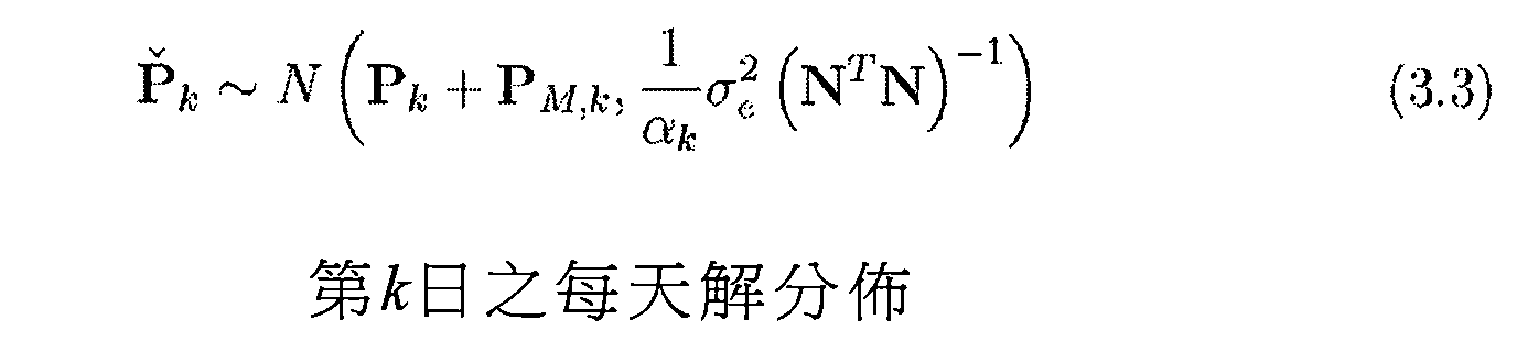
若每日使用相同雙差,則P M,k 變得固定且解之方差係僅歸因於所使用之雙差之數目及雜項誤差。儘管解將係有偏解,但對於其中相對移動係有關注價值的地面變形監測而言,此固定有偏將係不相關的,因此解將與吾人可能希望的一般好。 If the same double difference is used daily, P M,k becomes fixed and the variance of the solution is only due to the number of double differences used and miscellaneous errors. Although the solution will be biased, this fixed bias will be irrelevant for ground deformation monitoring where the relative mobile system has a value of concern, so the solution will be generally better than we might hope.
若吾人假定吾人每日不可獲得相同雙差,且實際上吾人隨機地取樣具有均一分佈之全部每日雙差之α百分比,則吾人僅僅具有假設明天將存在匹配雙差的今天獲得之雙差的機率,則吾人之解在足夠日情況下應如下分佈,使得PM,k之平均值更緊密類似於如吾人預期PM,k~N(P M ,(1-α k )

在此狀況下,在足夠日內吾人預期固定偏差,但具有大於之前的方差。吾人現在面臨兩個問題,第一問題顯然係方差的增大,而另一問題係每天多路徑偏差PM,k每日如何改變。GPS衛星重複時間相對於24小時每日滯後約四分鐘,因此若吾人可在整個全部白天時間期間獲得觀測,則吾人將預期每天多路徑偏差之緩慢改變。在此狀況下解可能看起來類似於就好像節點之實際方位在移動一般。作為實例,吾人進行以下模擬:吾人產生正態分佈多路徑、差量範數及雜項誤差,其中雜項誤差顯著小於多路徑誤差。吾人設定[1,1,1]之固定節點位置,計算針對全部曆元之可觀測量Φ,每日使用連續曆元之50%並每日將此移位0.3%,因此僅僅在白天時間期間模擬獲得觀測。下圖3.8展示使用吾人之模擬的解之x座標的繪圖。「Phat」係針對

比較起來,再次以相同參數運行相同模擬,惟改為每日使用確切相同之雙差除外。在圖3.9中標繪解之x座標。如可看到,當P M,k 固定時,剩餘方差係歸因於如方程式3.3中給出的雜項誤差。 In comparison, the same simulation is run again with the same parameters, except for the exact same double difference used daily. The x coordinate of the solution is plotted in Figure 3.9. As can be seen, when P M,k is fixed, the residual variance is due to the miscellaneous error as given in Equation 3.3.
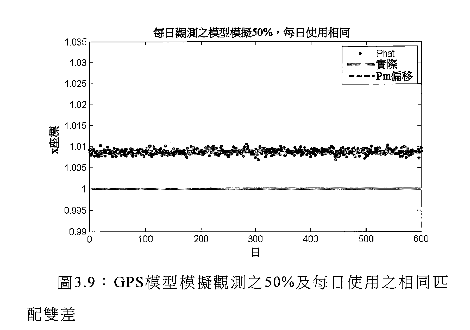
因此,吾人之情境係,短期內分佈可遵循方程式3.3,但在較長時期內分佈可遵循方程式3.4。 Therefore, the context of ours, the short-term distribution can follow Equation 3.3, but the distribution can follow Equation 3.4 for a longer period of time.
因此,為了縮減短期及長期之解方差,應一日24小時每秒一次採取觀測且每日使用相同之雙差處理資料。在運用永久供電之GPS接收器的情況下,非常易於每日獲得相同雙差且一日24小時每秒一次獲得,此係因為有足夠功率做到這一點。然而,在吾人之情境中,吾人不可僅僅在半夜接通吾人之GPS接收器,僅因為此處存在吾人需要匹配於吾人昨天使用之雙差的雙差以計算解。因此,對於吾人之情境,吾人將預期造成解方差增大之相當小的a值,而一秒一次取樣的永久供電高速率GPS接收器之情境將具有產生具有較少方差之解的大a值。吾人具有一具有大方差量之有偏估計器。吾人現在利用長期內P M,k 為隨機變數之事實。 Therefore, in order to reduce short-term and long-term solution variances, observations should be taken every second, 24 hours a day, and the same double-difference data should be used daily. In the case of a permanently powered GPS receiver, it is very easy to get the same double difference every day and get it once every 24 hours a day, because there is enough power to do this. However, in my situation, we can't just connect our GPS receiver in the middle of the night, just because there is a double difference between us that needs to match the double difference we used yesterday to calculate the solution. Therefore, for our situation, we will expect a fairly small value of a to increase the solution variance, and the situation of a permanently powered high rate GPS receiver sampled once per second will have a large a value that produces a solution with less variance. . We have a biased estimator with a large variance. We now use the fact that P M,k is a random variable in the long term.
使用吾人之來自方程式3.1的模型,吾人看到,對於第 k恆星日,以P B 及實際位置P k 評估之以循環為單位的殘餘可被書寫如下。 Using our model from Equation 3.1, we see that for the kth stellar day, the residual in cycles, evaluated by P B and the actual position P k , can be written as follows.

對於使用雙差之恆星差分化,今天之殘餘減去昨天之殘餘得到自昨天觀測以來的位移;此被書寫如下。 For the use of double-difference stellar differentiation, today's residual minus the residual of yesterday is obtained from the displacement observed yesterday; this is written as follows.

加性雜訊加倍,多路徑被移除,且使用LS得到昨天與今天之間的位移之估計

在許多此等天內平均化,吾人獲得下式。 After averaging over many of these days, we have the following formula.
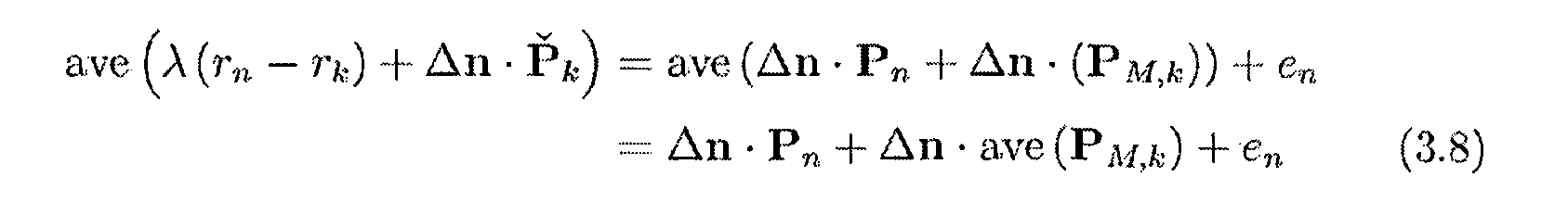
在足夠天內,吾人預期

因此,使用LS以獲得針對Pn之估計

其與吾人每日使用相同雙差時之分佈相同。當然,此為準確度及精確度之上限。若吾人考慮在許多此等天內平均化的算術平均值,則事情變得更複雜,此係因為僅僅存在吾人可首先形成殘餘差r n -r k 的機率。由此,吾人將條記號定義為所計算的算術平均值,可能時包括當天n。對於在第n日之r k ,此為


因此,使用方程式3.11之針對P n +

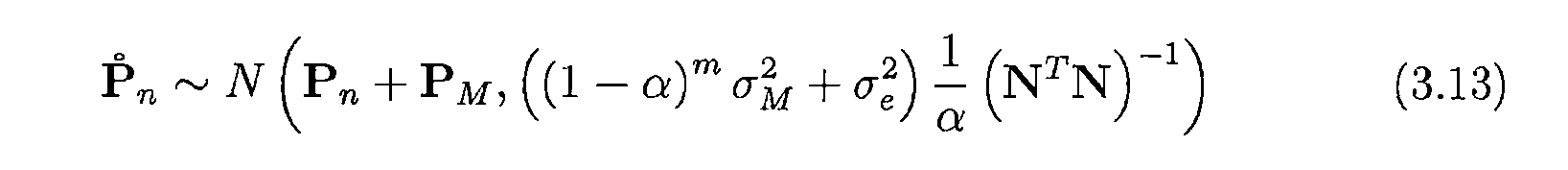
在吾人之情境中,吾人不可整日隨機地取樣α觀測,此係因為節點僅僅能夠在白天時間期間操作。若吾人將白天時間相對於整日之百分比定義為β,則吾人僅僅能夠隨機地取樣在白天時間內的觀測之α百分比(亦即,吾人獲得每日全部可能觀測的αβ百分比且此等中之全部係在白天時間)。每日,3指的觀測經移位四分鐘,因此第k日在時間上離開第n日更遠,能夠形成殘餘之機率下降。因此,運行平均值所針對的日愈多,

吾人不獲得g(α,β,m,δ)之顯式公式,實際上吾人僅注意,其與αβ及m正相關。 We do not obtain the explicit formula of g(α, β, m, δ) . In fact, we only pay attention to it, which is positively correlated with αβ and m .
在白天時間期間,節點獲得觀測,但在白天時期間未均一地獲得觀測。實際上,觀測大約在中午獲得較多且在早晨及夜晚獲得較少。然而,為使事情簡單,吾人不考慮此額外複雜情況且改為繼續假定在白天時間期間均一地獲取觀測。在紐西蘭之Paekakariki試驗台中在兩週時段內, 吾人量測在白天時間期間獲得的曆元之平均百分比為30%。因此,為了模擬,吾人使用α=0.3、β=0.5及δ=0.003。另外,吾人經由模擬移動節點[0.05 0.05 0.05]一半。吾人接著使用15天來進行恆星平均化(m=15)。在使用如前所述之相同模擬設定的情況下,吾人獲得圖3.10中之以下模擬結果。 During daylight hours, the nodes were observed, but were not uniformly observed during the daytime. In fact, observations get more at about noon and less in the morning and night. However, to make things simple, we do not consider this extra complication and instead continue to assume that observations are uniformly acquired during daylight hours. In the Paekakariki test bed in New Zealand during the two-week period, The average percentage of epochs we measured during daylight hours was 30%. Therefore, for the sake of simulation, we use α = 0.3, β = 0.5, and δ = 0.003. In addition, we passed the simulated mobile node [0.05 0.05 0.05] half. We then used 15 days for stellar averaging (m=15). In the case of using the same simulation settings as described above, we obtained the following simulation results in Figure 3.10.

如可看到,平均起來,存在微小解偏差且恆星濾波解進行顯著更好。作為比較,吾人再次進行相同模擬,但此次使用表示使用在白天時間期間之全部雙差的α=1。 As can be seen, on average, there is a slight solution bias and the stellar filter solution is significantly better. For comparison, we performed the same simulation again, but this time the use indicates that α = 1 is used for all double differences during daylight hours.

自圖3.10及3.11,吾人看到低頻雜訊分量及高頻雜訊分量。當使用日間恆星濾波時,低頻分量顯然相同,僅僅縮減高頻分量。低頻分量似乎為每一年重複並歸因於四分鐘每天移位的緩慢移動解偏差。低頻分量係有問題的,此係因為其看起來像GPS接收器節點隨時間緩慢移動。自此等圖,吾人亦看到,在長期過程中,日間恆星濾波僅僅在高頻雜訊分量具有顯著大於低頻分量之量值的量值時才有效。此等於說僅僅當正常解精確度之量值顯著大於每一年重複之緩慢移動偏差的量值時日間恆星濾波才在改良每天解準確度方面真正有效。 From Figure 3.10 and 3.11, we see low frequency noise components and high frequency noise components. When using daytime star filtering, the low frequency components are clearly the same, only the high frequency components are reduced. The low frequency component appears to be repeated for each year and is attributed to the slow moving solution deviation of the four minute shift per day. The low frequency component is problematic because it looks like the GPS receiver node moves slowly over time. From this graph, we also see that during the long-term process, daytime star filtering is only effective when the high-frequency noise component has a magnitude that is significantly larger than the magnitude of the low-frequency component. This is equivalent to saying that daytime stellar filtering is only really effective in improving the accuracy of daily solutions when the magnitude of the normal solution accuracy is significantly greater than the magnitude of the slow moving deviation repeated each year.
為檢查對於高頻雜訊之日間恆星濾波,吾人僅查看藉由使用一天差分化獲得的雜訊。為顯式


圖3.12僅展示在移除低頻雜訊分量後的高頻雜訊分量。如可看到,即使當使用在白天時間期間之全部雙差(α=1.0)時,在使用恆星濾波時仍存在高頻雜訊分量的縮減。然而,當僅僅使用白天時間期間雙差之分率(在此狀況下30%)時,高頻雜訊分量之改良更顯著。在此狀況下,使用白天時間期間之全部雙差造成高頻雜訊分量大約50%的縮減,而當使用白天時間期間雙差之僅僅30%時產生大約80%的高頻雜訊分量之縮減‘因此,當使用白天時期間之觀測之任何分率時,日間恆星濾波在縮減高頻雜訊分量方面有效。高頻分量的縮減當然係解精確度之改良。 Figure 3.12 shows only the high frequency noise components after removing the low frequency noise components. As can be seen, even when using the full double difference during daylight hours ( α = 1.0), there is still a reduction in high frequency noise components when using stellar filtering. However, the improvement of the high frequency noise component is more pronounced when only the rate of double difference during daylight hours (30% in this case) is used. In this case, the use of all double differences during daylight hours causes a reduction of about 50% of the high frequency noise components, and a reduction of about 80% of the high frequency noise components when using only 30% of the double difference during daylight hours. 'Therefore, daytime stellar filtering is effective in reducing high frequency noise components when using any fraction of the observations during the daytime period. The reduction in high-frequency components is of course an improvement in accuracy.
吾人最終檢查日間恆星濾波對解的效應,其中一日中之每一雙差用以計算解;在此狀況下,α=1、β=1且δ不相關。在經由模擬來運行此情形的情況下,吾人獲得圖3.13。 We finally examine the effect of daytime star filtering on the solution, where each double difference of the day is used to calculate the solution; in this case, α = 1, β = 1 and δ is irrelevant. In the case of running this scenario via simulation, we obtained Figure 3.13.

如所預期,在恆星濾波之前及之後的解係相同的且不存在準確度或精確度之改良。另外,不存在每年重複的緩慢移動解偏差。 As expected, the solutions before and after stellar filtering are identical and there is no improvement in accuracy or precision. In addition, there is no slow moving solution deviation repeated every year.
看起來當僅在整個白天時間獲得觀測時,日間恆星濾波改良精確度。當在白天時間期間採取僅僅幾個觀測時精確度之改良係最顯著。相比於正常解精確度之量值,日間恆星濾波取決於每年重複的緩慢移動偏差之量值而可或可不顯著改良準確度。正常解精確度之量值當然至少部分取決於在白天時間期間獲得的觀測之數目。 It seems that daytime stellar filtering improves accuracy when observations are taken only throughout the daylight hours. The improvement in accuracy when taking only a few observations during daylight hours is most pronounced. The daytime stellar filtering may or may not significantly improve the accuracy depending on the magnitude of the repeated slow moving deviations per year compared to the magnitude of the normal solution accuracy. The magnitude of the normal solution accuracy will of course depend, at least in part, on the number of observations obtained during daylight hours.
總而言之,吾人看到對於吾人之唯一間歇觀測情境由於使用恆星濾波而增加益處,另外若觀測不間歇,則間歇 觀測將對吾人不可用。另外,因為吾人之節點甚至在白天時間期間工作循環,因此相比於在吾人在整個白天時間連續獲得觀測的情況下吾人將獲得的益處,吾人自日間恆星濾波獲得更多益處然而,當僅使用白天時間觀測時,吾人亦觀測使用吾人之日間恆星濾波形式不可縮減之一年一次重複的緩慢移動解偏差。此緩慢移動偏差影響準確度而在短時間段內其似乎為固定偏差。 All in all, we have seen that the only intermittent observation scenario for our people has increased the benefits due to the use of stellar filtering, and if the observations are not intermittent, then intermittent Observations will not be available to us. In addition, because our nodes even work cycle during daylight hours, we benefit from daytime stellar filtering compared to the benefits that we will gain in the case of continuous observations throughout the daytime. However, when only used During the daytime observation, we also observed that the use of our day's stellar filtering form can not be reduced by one year of repeated slow moving solution deviation. This slow movement bias affects accuracy and appears to be a fixed deviation over a short period of time.
吾人現在繼續校驗當在使用真實壽命觀測的情況下間歇地獲得觀測時日間恆星濾波確實改良解。 We continue to verify that daytime stellar filtering does improve the solution when observations are obtained intermittently using real life observations.
3.3.1模擬驗證3.3.1 Simulation verification
對於基於吾人之多路徑模型的模擬,吾人已看到,對於吾人之特定唯一硬體,觀測僅僅在白天期間且甚至接著僅僅間歇地可用,吾人預測吾人之解應採取圖3.10中看到的結果。首先,吾人預測恆星濾波器應即刻對節點位置之改變作出反應且解應匹配於所進行的實體位移之改變。其次,吾人預測吾人當間歇地獲得觀測時使用此章中描述之日間恆星濾波確實獲得每天解精確度之改良,且當使用連續高速率觀測時不可得到改良。第三,應存在吾人之日間恆星濾波不可縮減之將每年重複一次的解偏差之緩慢改變。第三預測吾人可不校驗,此係因為其將需要靜態節點之多於一年的觀測。第四,當使用比許多白天觀測更少的白天觀測時,任何改良更顯著。第四預測吾人此處不驗證。 For the simulation based on our multi-path model, we have seen that for our particular unique hardware, the observations are only available during the day and even then only intermittently, and we predict that our solution should take the results seen in Figure 3.10. . First, we predict that the stellar filter should react immediately to changes in node position and the response should match the change in the physical displacement being performed. Secondly, we predict that the daytime stellar filtering described in this chapter will improve the daily solution accuracy when we obtain observations intermittently, and cannot be improved when using continuous high-rate observations. Third, there should be a slow change in the deviation of the solution that will be repeated every year for our day's stellar filtering. The third prediction may not be verified by us because it will require more than one year of observation of static nodes. Fourth, any improvement is more pronounced when using less daytime observations than many daytime observations. The fourth forecast is not verified by us here.
前兩個關於回應及改良之預測吾人驗證如下。 The first two predictions about response and improvement are verified as follows.
3.3.1.1 恆星回應3.3.1.1 Stellar response
運用如第5章硬體中所描述但經修改成關斷連續電力供應器之節點運行實驗。天線置放於屋頂上且接收器安裝在屋簷下方避免直射日光及元件影響,基準為大約10m。運用連續功率,有可能獲得最高可能準確度,且判定恆星解當節點之基礎移動改變時是否瞬時移動,另外,判定恆星解之改變是否與基礎移動一致。節點之天線在NNW方向中且稍微向下移動;首先20±2mm且接著5±1mm。使用日之每一曆元,相對於計算解所針對的日,標繪解之主要主分量。圖3.14展示此繪圖,其中恆星濾波器具有15日之移動窗時間段。 Run the experiment using a node as described in Chapter 5, Hardware, modified to turn off the continuous power supply. The antenna is placed on the roof and the receiver is mounted under the eaves to avoid direct sunlight and component effects. The reference is approximately 10m. With continuous power, it is possible to obtain the highest possible accuracy, and determine whether the stellar solution moves instantaneously when the base motion of the node changes, and determines whether the change of the stellar solution is consistent with the base motion. The antenna of the node moves in the NNW direction and moves slightly downward; first 20 ± 2 mm and then 5 ± 1 mm. Using each epoch of the day, plot the main principal component of the solution relative to the day against which the solution is calculated. Figure 3.14 shows this plot where the star filter has a 15 day moving window time period.

節點之天線大約在第357日之中午移動;此可在上圖3.14中看到,此係因為既不在如在之前位置處獲得之一些雙差之-0.01處亦不在如在之後位置處獲得之其他雙差之0.01處的點,造成最終解既不為前者亦不為後者。在第368 日下午7點處進行5mm移動。如可看到,恆星濾波器對如所預期之移動瞬時回應,但不同於模擬,對於類似2cm移動之較大移動,恆星解低估移動且緩慢調整至新的位置。此係有意義的,此係因為多路徑隨位置而變,因此,用於恆星解之先前日具有稍微不正確多路徑資訊。為了模擬,吾人假定多路徑獨立於位置,因此為何吾人未在圖3.10中看到吾人在圖3.14中看到的恆星解之緩慢線性上升。對於5mm運動,恆星濾波器在2cm移動之前不具有足夠時間捨棄全部觀測,當在5mm移動之後計算第一恆星解時在進行2cm移動之前吾人使用4日。自圖3.14,吾人藉由在進行移動之前檢查恆星解及在進行移動之前獲得方位之估計而估計恆星解之移動的量值;按時間次序,此等值為-9.9±0.2mm、8.0±0.4mm且12.6±0.2mm,具有95%可信度。自此,吾人估計第一移動為17.8±0.6mm而第二移動為4.6±0.6mm,兩者具有95%可信度;因此,兩者估計與自使用尺子獲得的估計一致。對於在此特定試驗位點處在短暫時間框內的相對較小移動,此至少展示盡吾人所能可判定的恆星解與GPS天線自身之基礎移動一致。 The antenna of the node moves about noon on the 357th day; this can be seen in Figure 3.14 above, because it is neither at the 0.01 of the double difference obtained at the previous position nor at the position as after. The point of the other double difference of 0.01 makes the final solution neither the former nor the latter. A 5mm move was made at 7 pm on the 368th day. As can be seen, the stellar filter responds instantaneously to the expected motion, but unlike the simulation, for larger movements like 2 cm movement, the stellar solution underestimates the movement and slowly adjusts to the new position. This makes sense because this multipath varies with location, so the previous day for the stellar solution has slightly incorrect multipath information. For the sake of simulation, we assume that the multipath is independent of location, so why did we not see the slow linear rise of the stellar solution we saw in Figure 3.14 in Figure 3.10. For 5 mm motion, the stellar filter does not have enough time to discard all observations before the 2 cm movement, and when the first stellar solution is calculated after 5 mm movement, we use 4 days before the 2 cm movement. From Figure 3.14, we estimate the magnitude of the movement of the stellar solution by examining the stellar solution before moving and obtaining an estimate of the orientation before moving; in chronological order, the values are -9.9 ± 0.2 mm, 8.0 ± 0.4 Mm and 12.6 ± 0.2 mm with 95% confidence. Since then, we have estimated that the first movement is 17.8 ± 0.6 mm and the second movement is 4.6 ± 0.6 mm, both with 95% confidence; therefore, the two estimates are consistent with the estimates obtained from the use of the ruler. For relatively small movements within a short time frame at this particular test site, this at least shows that the stellar solution that can be determined by us is consistent with the base movement of the GPS antenna itself.
3.3.1.2 恆星解改良3.3.1.2 Stellar solution improvement
全部吾人之靜態真實壽命觀測之試驗係相對短暫的,持續不大於幾個月。此意謂吾人能夠看到解之高頻率而非低頻率。此意謂吾人可僅僅觀測解精確度改良而非準確度改良。當然,吾人預測之上述情形係日間恆星濾波將展示清晰改良的情況。 The test of all our static real life observations is relatively short and lasts no more than a few months. This means that we can see the high frequency of the solution rather than the low frequency. This means that we can only observe the accuracy improvement rather than the accuracy improvement. Of course, the above-mentioned situation predicted by us is that the daytime stellar filtering will show a clear improvement.
根據吾人之多路徑模型,當每日使用相同曆元以獲得解時(諸如當使用永久供電GPS接收器取得高速率觀測時)獲得的解,日間恆星濾波應不具有效應。然而,自圖3.14來看,此似乎並非如此。若吾人僅考慮2cm移動之前及在5mm移動之後的日,則吾人看到大約30%之2DRMS的改良。吾人推理吾人在吾人之模擬中並未預測的此改良可係由於衛星重複週期並非確切為24小時246秒而實際上對於每一衛星係不同的,從而造成雙差之多路徑並不完全每日重複的事實。當使用來自永久供電接收器之全部觀測時,繪製解之前兩個主分量,獲得圖3.15,其中可更清晰地看到此改良。 According to our multipath model, daytime stellar filtering should have no effect when the same epoch is used daily to obtain a solution (such as when using a permanently powered GPS receiver to achieve high rate observations). However, as seen in Figure 3.14, this does not seem to be the case. If we only consider the day before the 2cm movement and after the 5mm movement, then we see an improvement of about 30% of 2DRMS. We reason that this improvement that we did not predict in our simulations may be due to the fact that the satellite repetition period is not exactly 24 hours and 246 seconds but is actually different for each satellite system, resulting in a double-difference path that is not completely daily. Duplicate facts. When using all observations from the permanent power receiver, plot the two previous principal components and obtain Figure 3.15, which can be seen more clearly.
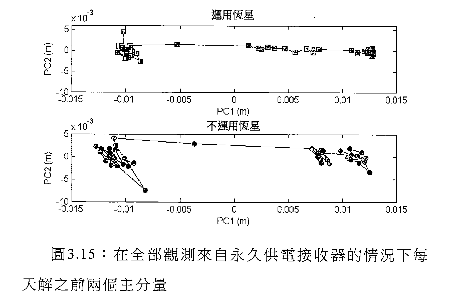
為了研究在觀測不連續時的改良,吾人使用自連續供電節點獲得的觀測且僅僅選擇具有與在附近置放的太陽能供電GPS節點相同之時間的觀測。因此,永久供電觀測之 作用中的分佈將匹配於自太陽能供電GPS節點自身獲得之觀測的分佈。以此方式,吾人消除位置對改良之可能相依性。再次,僅考慮在2cm移動之前及在5mm移動之後的日,在此狀況下,吾人獲得大約60%之2DRMS的改良。此改良為當一秒一次地連續獲得觀測時獲得的未預期改良之雙倍。在太陽能供電GPS接收器節點獲得觀測的情況下,當僅僅使用來自永久供電接收器之觀測時,繪製解之前兩個主分量,吾人獲得可看到此改良之以下繪圖。 In order to study the improvement in the observation discontinuity, we used the observations obtained from the continuous power supply node and only selected the observations with the same time as the solar powered GPS nodes placed nearby. Therefore, permanent power supply observation The distribution in action will match the distribution of observations obtained from the solar powered GPS node itself. In this way, we eliminate the possible dependence of location on improvement. Again, considering only the day before the 2 cm movement and after the 5 mm movement, in this case, we obtained an improvement of about 60% of 2DRMS. This improvement is double the unexpected improvement obtained when the observation is continuously obtained once in a second. In the case where the solar powered GPS receiver node is observing, when only the observations from the permanent power receiver are used, the first two principal components are plotted, and we obtain the following plots where this improvement can be seen.

如自此等圖(3.15及3.16)兩者可看到,使用恆星濾波產生彼此相當類似的解。在第二圖(3.16)中在不使用恆星濾波之情況下的5mm階躍不可被容易地判定而當使用恆星濾波時其易於判定。視需要,在白天時間期間當使用間歇觀測時的改良顯著大於當使用永久供電GPS接收器時獲得之改良。 As can be seen from the figures (3.15 and 3.16), the use of stellar filtering produces solutions that are quite similar to each other. The 5 mm step in the second graph (3.16) without the use of stellar filtering cannot be easily determined and is easy to determine when using stellar filtering. The improvement when using intermittent observations during daylight hours is significantly greater than the improvement obtained when using permanently powered GPS receivers, as needed.
最終,對於置放於Paekakariki試驗台處且保持22天的實際太陽能供電GPS接收器,吾人比較恆星解與非恆星解。此GPS接收器節點為如第5章中所描述的節點。可在第68頁上之圖3.17中看到解之鳥眼視圖。 Finally, for the actual solar-powered GPS receivers placed at the Paekakariki test rig for 22 days, we compared stellar solutions with non-stellar solutions. This GPS receiver node is a node as described in Chapter 5. The bird's eye view of the solution can be seen in Figure 3.17 on page 68.

如可看到,恆星濾波對解精確度有顯著效應。獲得自5.6mm至2.8mm之2DRMS的大約50%之改良。僅僅使用在太陽能供電GPS接收器節點在作用中時取得之觀測的情況下的2DRMS之此改良百分比與在使用永久供電GPS接收器時吾人看到之改良相當。 As can be seen, stellar filtering has a significant effect on the accuracy of the solution. Approximately 50% improvement in 2DRMS from 5.6 mm to 2.8 mm was obtained. The percentage improvement of 2DRMS in the case of using only observations taken while the solar powered GPS receiver node is active is comparable to the improvement seen by us when using a permanently powered GPS receiver.
3.4 天內恆星濾波3.4 days of stellar filtering
天內恆星濾波解(天內解)為使用除了在自身所討論之秒中觀測以外在其他日中之觀測的基於曆元之解;其他日可未必為連續日。 The stellar filtering solution (in-day solution) is an epoch-based solution using observations in other days other than observations in the second discussed in the day; other days may not be consecutive days.
天內恆星濾波並非為吾人之主要關注,此係因為吾人 之系統並不與諸如RTK之即時系統競爭。另外,進行使用每天解集中於長期地面變形量測的決策並很好進行此決策。然而,不存在吾人之系統為何不可擴展至基於曆元之解的原因但將需要更多工作來研究此類型解。在該章節中,吾人使用過去資訊及當前曆元來計算解而簡單檢查天內解。 The stellar filtering in the day is not the main concern of our people. This is because of my The system does not compete with real-time systems such as RTK. In addition, the decision to use the daily defocusing on long-term ground deformation measurements is made and this decision is made very well. However, there is no reason why our system cannot be extended to epoch-based solutions but more work will be needed to study this type of solution. In this chapter, we use the past information and the current epoch to calculate the solution and simply check the solution within a day.
計算天內演算法之多路徑估計係藉由使用先前日而進行,其中節點之位置不變,吾人具有先前日之日間恆星解。此等日間解係非常準確,其中殘餘主要由多路徑組成且因此吾人可計算彼等先前日的多路徑。吾人具有的此多路徑資訊接著使用簡單幾何平均化而組合以建立多路徑映圖,吾人可將當前日之任何雙差校正成多路徑映圖。吾人使用有偏位置將雙差變成殘餘,校正殘餘,接著將此等轉換回雙差(最小平方可用於雙差),而非校正雙差自身。此經如此進行,以便避免使用如在日間恆星濾波演算法中進行的經解開雙差值。假定吾人具有真實多路徑M之估計為M',最初對於經解開雙差,此程序經概括如下。 The multipath estimation of the algorithm in the calculation day is performed by using the previous day, where the position of the node is unchanged, and we have the star solution of the previous day. These daytime solutions are very accurate, where the residuals are primarily composed of multiple paths and therefore we can calculate their previous day's multipath. This multipath information that we have is then combined using simple geometric averaging to create a multipath map, and we can correct any double difference for the current day to a multipath map. We use the biased position to turn the double difference into a residual, correct the residual, and then convert this back to double difference (the least square can be used for double difference) instead of correcting the double difference itself. This is done in order to avoid using the unwrapped double difference as performed in the daytime stellar filtering algorithm. Assuming that we have an estimate of true multipath M as M' , this procedure is summarized as follows for the unwrapped double difference.
˙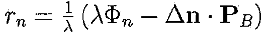
˙
˙
˙
˙
為了獲得多路徑估計M',幾何平均化歸因於簡單實施方案而使用並概括如下。 To obtain a multipath estimate M' , geometric averaging is used and summarized as follows due to a simple implementation.
˙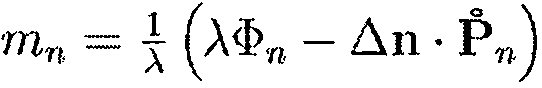

˙
因此,兩個方程式用於吾人之天內恆星濾波;基於昨天之多路徑估計的經校正方程式及多路徑估計之更新方程式,此等兩個方程式為方程式(3.15)及(3.16)(並非基礎)。 Therefore, the two equations are used for stellar filtering in our day; based on the corrected equations of yesterday's multipath estimation and the updated equations for multipath estimation, these two equations are equations (3.15) and (3.16) (not the basis). .

吾人改為選擇使用包裝殘餘以便避免如吾人在日間恆星濾波中進行的循環滑移,而非使用解開殘餘。在使用包裝殘餘後,就可如以下演算法中所列出而描述吾人之演算法。 Instead of using the unwrapping residue, we chose to use the packaging residue instead of the cyclic slip as we did in the daytime star filtering. After using the package remnants, our algorithm can be described as listed in the following algorithm.

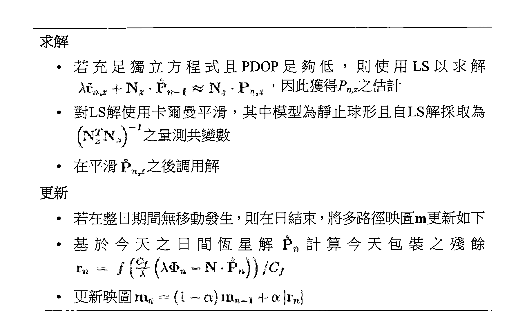
3.4.1天內恆星濾波改良Improved star filtering in 3.4.1 days
吾人將基於曆元之解與或不與天內恆星濾波比較。下圖3.18展示在不對藉由如硬體章-硬體(Hardware)中所描述的吾人之無線太陽能供電GPS接收器節點自廬山試驗台獲得之觀測進行天內恆星濾波之情況下的基於曆元之解。不處理具有不充足方程式及/或過多方位精確度因子(PDOP)之曆元之解。另外,對解進行卡爾曼平滑,其中模型為靜止球形及自LS解採取為(
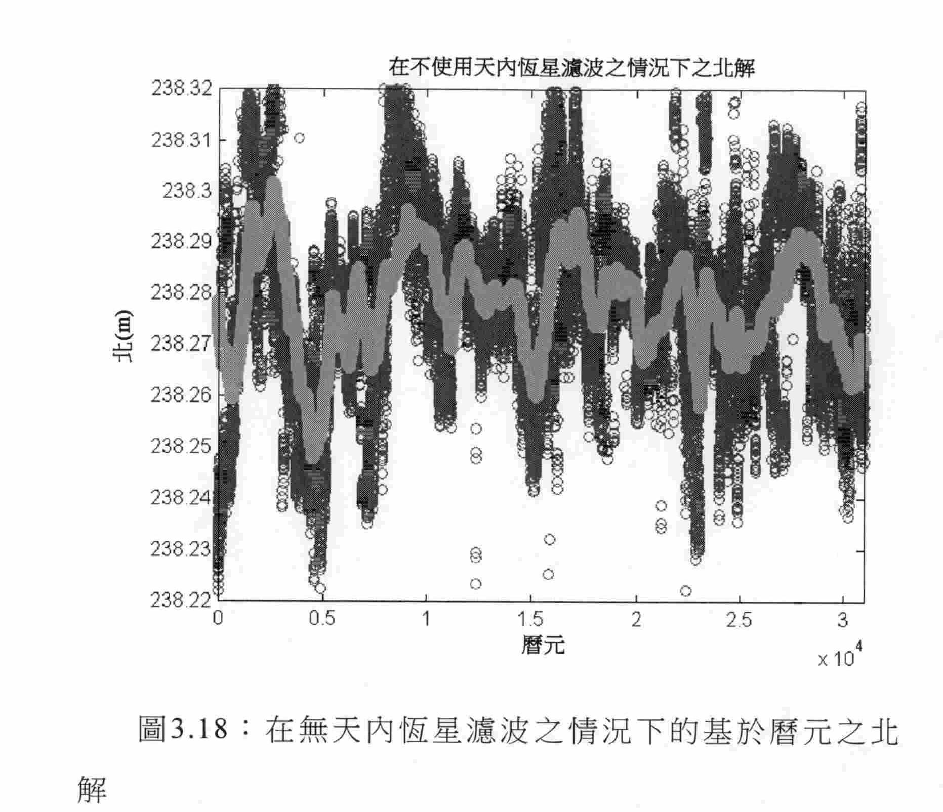
下圖3.19展示如用於圖3.18但實際上運用天內恆星濾波之相同觀測。演算法預先具有10日以調整其多路徑映圖。 Figure 3.19 below shows the same observations as used in Figure 3.18 but actually using stellar filtering for a day. The algorithm has 10 days in advance to adjust its multipath map.

如可看到,多路徑效應已在每秒基礎上顯著縮減。對於解自身,觀測到2DRMS準確度的大約60%之改良,而一旦經由卡爾曼濾波器運行解自身就觀測到大約80%之改良。對於此測試,2DRMS精確度量測列表於下表(表3.1)中。 As can be seen, the multipath effect has been significantly reduced on a per second basis. For the solution itself, an improvement of about 60% of the 2D RMS accuracy was observed, and an improvement of about 80% was observed once the solution itself was run via the Kalman filter. For this test, the 2DRMS accurate measurement is listed in the table below (Table 3.1).

3.4.2天內恆星濾波回應Stellar filtering response within 3.4.2 days
3.4.2.1 5mm永久功率3.4.2.1 5mm permanent power
首先使用如章節3.3.1.1中看到的永久供電GPS接收器 之5mm移動檢查天內恆星濾波對於移動的回應。首先,在運用應用於解之一小時移動平均濾波器情況下在圖3.20中標繪在四日內之在無天內恆星濾波之情況下的移動之主要水平分量。 First use the permanently powered GPS receiver as seen in section 3.3.1.1 The 5mm movement checks the response of the star filter to the movement during the day. First, the main horizontal component of the movement in the case of no-day star filtering within four days is plotted in Figure 3.20 using the one-hour moving average filter applied.
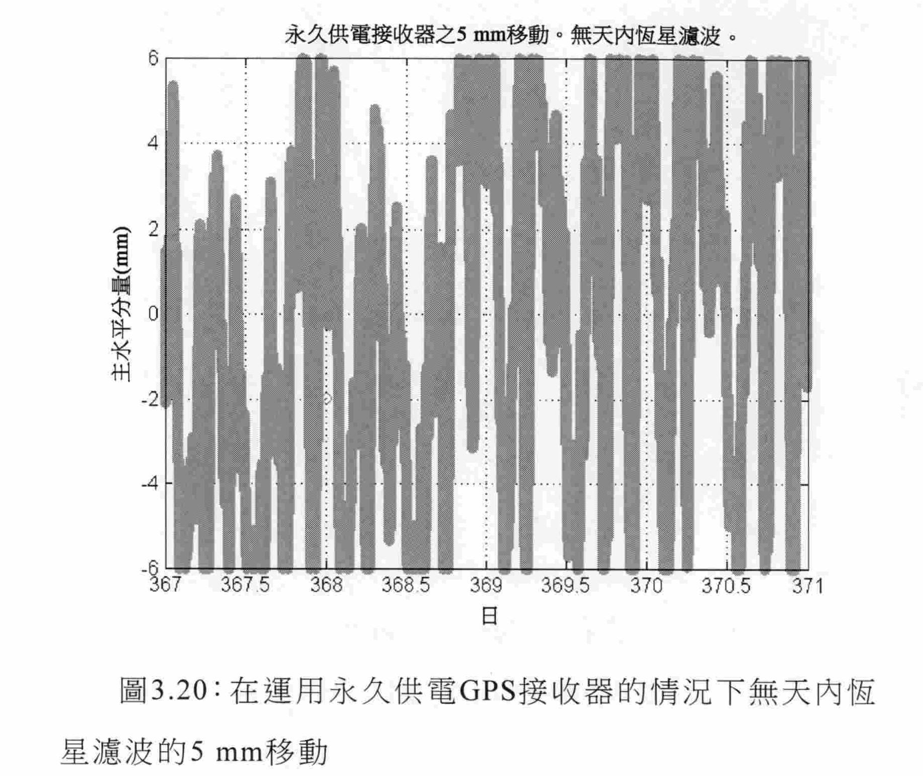
再次相同地但在α為0.25之情況下藉由添加天內恆星濾波而處理相同資料;可在具有與先前圖(圖3.20)相同之標度的圖3.21中看到結果。 Again, the same data is processed again by adding intra-day star filtering if α is 0.25; the results can be seen in Figure 3.21 with the same scale as the previous figure (Figure 3.20).
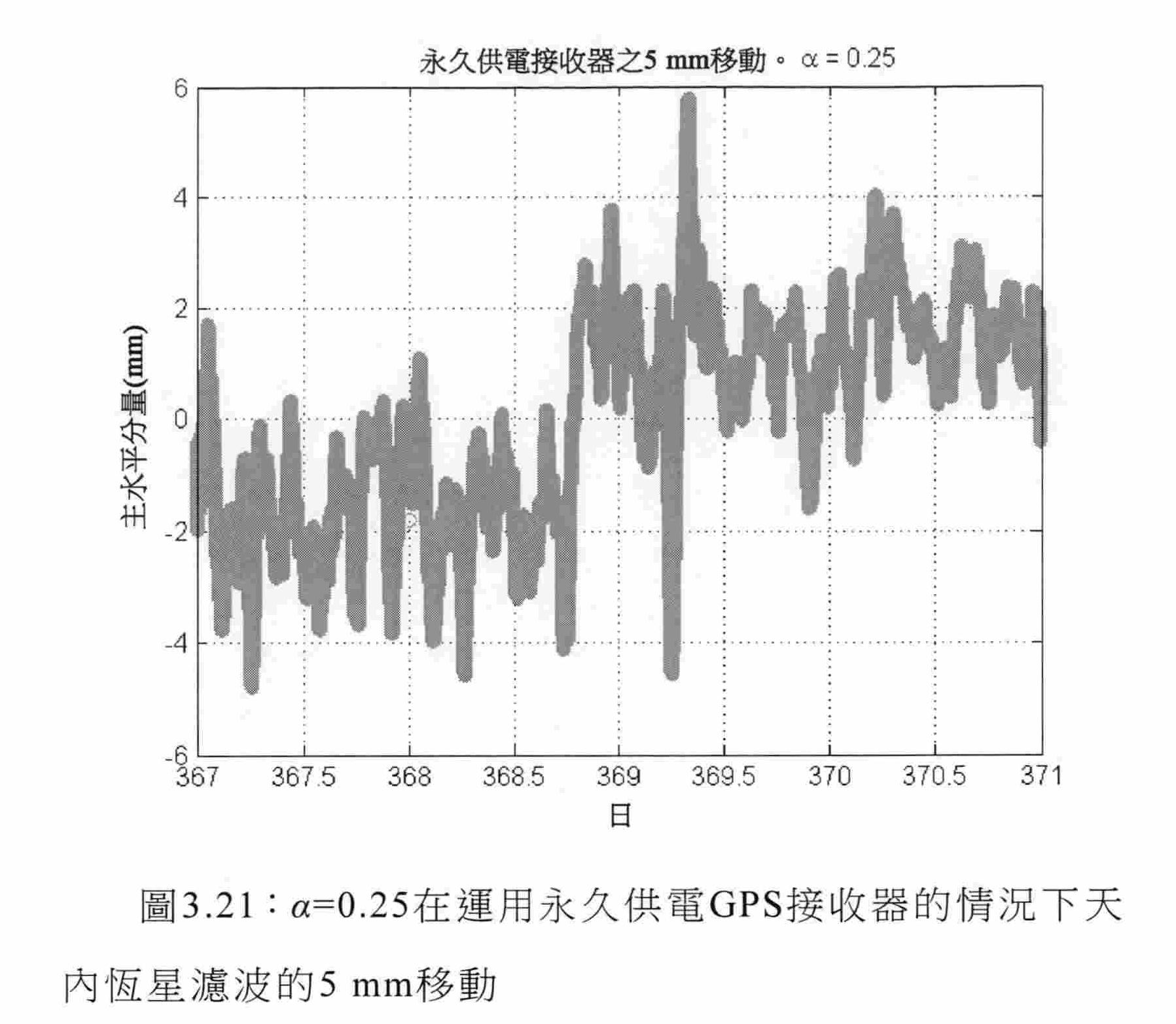
如可看到‘在無天內恆星濾波之情況下,非常難以判定移動已發生,而運用天內恆星濾波,可更容易地偵測移動。藉由圖3.21判定如在1月3日之下午6點與下午8點之間的移動之時間,而實際移動之時間係在1月3日的下午7:10。 As you can see, ‘without a day of star filtering, it’s very difficult to determine that a movement has occurred, and using a day of star filtering makes it easier to detect movement. The time of the move between 6 pm and 8 pm on January 3 is determined by Figure 3.21, and the actual movement time is at 7:10 pm on January 3.
對圖3.21進行核心密度估計(KDE),獲得圖3.22。 Core density estimation (KDE) is performed in Figure 3.21, and Figure 3.22 is obtained.

圖3.22展示移動為大約3.2mm。如由傾角儀所量測的屋頂之坡度為15°,因此總移動應為離5mm之期望值1.7mm的3.3mm。 Figure 3.22 shows that the movement is approximately 3.2 mm. If the slope of the roof measured by the inclinometer is 15°, the total movement should be 3.3 mm from the expected value of 1.7 mm from 5 mm.
最終,再次進行天內恆星濾波,但此次使用為1之α值。可在圖3.23中看到此之結果。 Finally, the stellar filtering is performed again in the day, but this time it is the alpha value of 1. This can be seen in Figure 3.23.

圖3.21與圖3.23之間的差為脈衝回應。可在圖3.23中看到,在移動之後恰好一天存在圖3.21中並不顯著的尖銳谷。此如當α=1時用於獲得多路徑估計的僅僅前一日所預期且當獲得該多路徑估計時的要求係在彼日中節點靜止,此顯然並非當節點移動時之狀況。當α=0.25時,較少多路徑估計係基於前一日且因此為何吾人不注意在圖3.21中之實際移動之後的一天的任何谷。 The difference between Figure 3.21 and Figure 3.23 is the impulse response. As can be seen in Figure 3.23, there is a sharp valley that is not significant in Figure 3.21 just one day after the move. This is as expected only for the previous day when α = 1 is used to obtain the multipath estimate and when the multipath estimate is obtained, the node is stationary in the day, which is obviously not the condition when the node moves. When α = 0.25, the less multipath estimation is based on the previous day and therefore why we are not paying attention to any valley of the day after the actual movement in Figure 3.21.
3.4.2.2 2cm太陽能3.4.2.2 2cm solar energy
在紐西蘭之Paekakariki試驗台處進行在四天內使用太陽能供電節點之階躍回應測試。第一日係記錄多路徑映圖,第二日係確保多路徑減輕成功並獲得控制,第三日係 其中節點被移動,且第四日係監測天內恆星濾波器之回應。為1之α用於天內恆星濾波演算法,此意謂有限脈衝回應且在階躍之後僅僅一日將需要看到任何類型之回應。 A step response test using a solar powered node within four days was conducted at the Paekakariki test bed in New Zealand. The first day records the multipath map, and the second day ensures that the multipath is mitigated successfully and gains control. On the third day, the nodes are moved, and the fourth day monitors the response of the stellar filter during the day. The alpha of 1 is used for the stellar filtering algorithm in the day, which means a finite impulse response and will only need to see any type of response after only one day after the step.
節點之移動係在大約北方向中且如藉由尺子所量測之移動為大約2cm。在2014年12月5日之上午11:06進行移動。使用天內恆星濾波演算法,看到在大約上午11點開始並在下午12點完成的線性移動,但因為解僅僅係間歇的因而難以判定。因為移動係瞬時的,因此吾人可以說線性移動之第一跡象應在如由吾人所引起的實際瞬時移動處或在進行如由吾人所引起的實際瞬時移動之後。因此,吾人自天內恆星濾波演算法判定瞬時移動發生在與如由吾人進行之實際移動一致的大約上午11點。 The movement of the nodes is in the approximately north direction and is about 2 cm as measured by the ruler. Moved at 11:06 am on December 5, 2014. Using the stellar filtering algorithm for a day, I saw a linear movement that started around 11 am and completed at 12 pm, but it was difficult to determine because the solution was only intermittent. Since the movement is instantaneous, it can be said that the first indication of linear movement should be at the actual instantaneous movement as caused by our own or after the actual instantaneous movement as caused by our own. Therefore, from day to day, the stellar filtering algorithm determines that the instantaneous movement occurs at approximately 11 am, which is consistent with the actual movement as performed by us.
圖3.24展示在第二至第四日(包括首尾)內的解之密度。如可看到,存在在幾乎正北方向中之清晰移動;如自下圖3.24量測的兩個位置之間的位移為大約1.8cm。此位移稍微小於如使用尺子量測的2cm。 Figure 3.24 shows the density of the solution in the second to fourth days (both inclusive). As can be seen, there is a clear movement in the almost north direction; the displacement between the two positions as measured from Figure 3.24 below is approximately 1.8 cm. This displacement is slightly less than 2 cm as measured using a ruler.
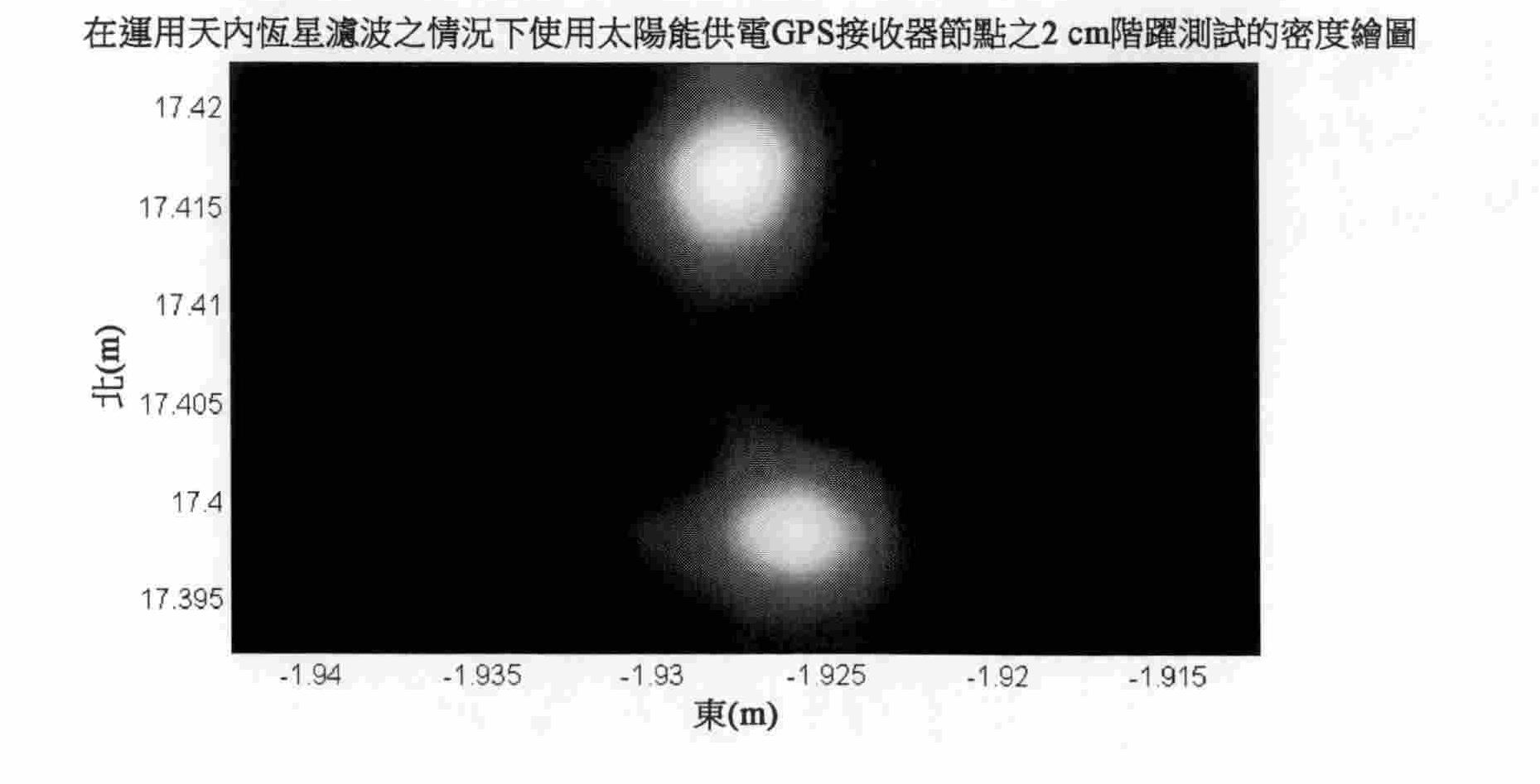
下圖3.25展示關於進行移動時之時間的水平解之主要主分量。 Figure 3.25 below shows the main principal component of the horizontal solution for the time when the movement was made.
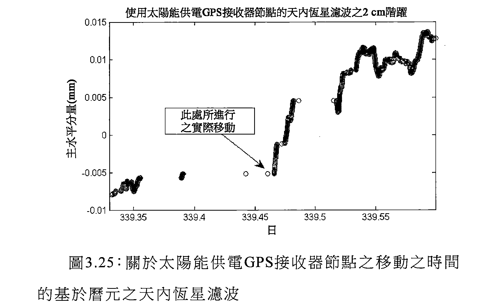
如可看到,使用太陽能供電GPS接收器之間歇性質意謂若移動在GPS接收器並未接通或主動地獲得適用之觀測時發生,則直至在GPS接收器再次變得在作用中且獲得足夠數目個觀測之後移動才將被量測。 As can be seen, the intermittent nature of using a solar powered GPS receiver means that if the movement occurs when the GPS receiver is not turned on or actively obtains the applicable observations, then until the GPS receiver becomes active again and gets After a sufficient number of observations, the movement will be measured.
下圖3.26展示全部四天內的水平解之主要主分量。 Figure 3.26 below shows the main principal components of the horizontal solution for all four days.

作為比較,在不使用天內恆星濾波之情況下,第2日至第4日(包括首尾)之解的密度如前在圖3.24中但在無天內恆星濾波之情況下被標繪;此可在圖3.27中看到,其中繪圖之標度與圖3.24中相同。如在此狀況下可看到,不可能判定兩個位置。 For comparison, the density of the solution from day 2 to day 4 (including the head and tail) is plotted as shown in Figure 3.24 but without star filtering in the day without star filtering in the day; This can be seen in Figure 3.27, where the scale of the plot is the same as in Figure 3.24. As can be seen in this situation, it is not possible to determine two locations.

演算法比較Algorithm comparison
4.1 網路頻寬比較之縮減4.1 Reduction of network bandwidth comparison
GPS接收器輸出以下各者以用於精確度應用;L1虛擬距離可觀測量、L1相位可觀測量、L1多普勒可觀測量、L1信號強度可觀測量、失鎖識別符、品質識別符、衛星數目,及如藉由接收器之時脈給出的觀測時間。通常,發出更大量資料。雖然並不需要全部用於高準確度解,但虛擬距離、相位、衛星編號及時間將被視為某種高準確度解所需要的最小需求。 The GPS receiver outputs the following for accuracy applications; L1 virtual distance observables, L1 phase observables, L1 Doppler observables, L1 signal strength observables, loss of lock identifiers, quality identifiers, number of satellites, And the observation time given by the clock of the receiver. Usually, a larger amount of information is sent. Although not all for high-accuracy solutions, virtual distance, phase, satellite number, and time will be considered the minimum requirements for a high-accuracy solution.
資料大小之典型分解將為:虛擬距離、相位及時間全部為八位元組值;多普勒為四位元組;信號強度為一位元組;失鎖識別符為一位元組;品質識別符為一位元組;且衛星編號為一位元組。 The typical decomposition of data size will be: virtual distance, phase and time are all octet values; Doppler is four bytes; signal strength is one tuple; loss lock identifier is one tuple; quality The identifier is a tuple; and the satellite number is a tuple.
對於一曆元,通常一次將僅僅發出對不同衛星之n多個觀測。表4.1展示在此情形下發送的位元組之數目的分解

雖然對於一個曆元n可在任意處為0至32,但典型值將 介於4與10之間。假定10為上限,此將每一節點一秒產生高達248位元組。 Although it can be anywhere from 0 to 32 for an epoch n , a typical value will be between 4 and 10. Assuming 10 is the upper limit, this will result in up to 248 bytes per second per node.
低功率無線網路解具有相對緩慢資料速率,從而限制通道容量。此部分地歸因於較慢資料速率意謂對於相同數量功率及相同調變方法之較大傳輸距離的事實。另外,節點之較少頻寬要求產生較低曆元資料丟失,因此減輕有損通道之效應。因為通道容量、功率使用及曆元丟失,最小化節點實際上發送的資料量係有利的。較少頻寬要求之另一優點為更多節點可佔據通道,從而在給定通道上增加網路中之節點的數目。 Low power wireless network solutions have a relatively slow data rate, limiting channel capacity. This is due in part to the fact that the slower data rate means a larger transmission distance for the same amount of power and the same modulation method. In addition, the less bandwidth of the nodes requires lower epoch data loss, thus mitigating the effects of lossy channels. Because channel capacity, power usage, and epochs are lost, it is advantageous to minimize the amount of data that the node actually sends. Another advantage of less bandwidth requirements is that more nodes can occupy the channel, increasing the number of nodes in the network on a given channel.
為縮減來自GPS接收器自身之資料量,CFFS演算法中之一些係實施於節點自身上,因此改變經由RF鏈結發送之資料。演算法2.1為在節點上運行之演算法。 To reduce the amount of data from the GPS receiver itself, some of the CFFS algorithms are implemented on the node itself, thus changing the data sent via the RF link. Algorithm 2.1 is an algorithm that runs on a node.
外推之包裝相位可觀測量、衛星編號及秒對準時間為傳回之主要變數。另外,偶爾地傳回基於近似碼之解;此可如一日一次或兩次地不頻繁進行。此係如此不頻繁,以致其對所需要頻寬無有效貢獻且可被忽略。 The extrapolated package phase observable, satellite number and second alignment time are the main variables of the return. In addition, the solution based on the approximation code is occasionally returned; this can be done infrequently once or twice a day. This is so infrequent that it does not contribute effectively to the required bandwidth and can be ignored.
演算法之主要部分經由網際網路或某一其他機制對時間有近似瞭解且節點區段已將時間對準至秒。若吾人假定演算法之主要部分知曉一分鐘內之時間,且演算法之節點區段與主要區段之間的潛時亦小於一分鐘,則演算法之主要部分有可能在節點區段僅發送時間之模256版本之情況下計算觀測之時間。因為此等時序要求非常容易達成,因此需要每曆元僅僅一個位元組在演算法之節點與主要區段 之間發送。 The main part of the algorithm has an approximate understanding of time via the Internet or some other mechanism and the node segment has time aligned to seconds. If we assume that the main part of the algorithm knows the time within one minute and the latency between the node segment and the main segment of the algorithm is less than one minute, then the main part of the algorithm may only be sent in the node segment. The time of observation is calculated in the case of the 256 version of time. Because these timing requirements are very easy to achieve, only one byte per epoch is required at the node and main section of the algorithm. Sent between.
包裝之相位可觀測量移除相位可觀測量之整數部分且留下零與一之間的數目。此將需要一之分率之準確度的約20,000之數目轉換至需要一之分率的約一之數目;此意謂吾人僅僅需要幾個位元組以恰好準確地編碼剩餘資訊且出於吾人之目的2位元組應係足夠的。2位元組意謂吾人具有約65,000分之一的相位解析度。 The phase of the package is appreciable to remove the integer portion of the phase observable and leave a number between zero and one. This will require a number of approximately 20,000 of the accuracy of the rate to be converted to a number that requires a rate of one; this means that we only need a few bytes to accurately encode the remaining information and The purpose of the 2-byte should be sufficient. A 2-byte means that we have a phase resolution of about 65,000.
下表展示可發送用於CFFS演算法節點的位元組之絕對最小數目之分解。 The following table shows the decomposition of the absolute minimum number of bytes that can be sent for a CFFS algorithm node.
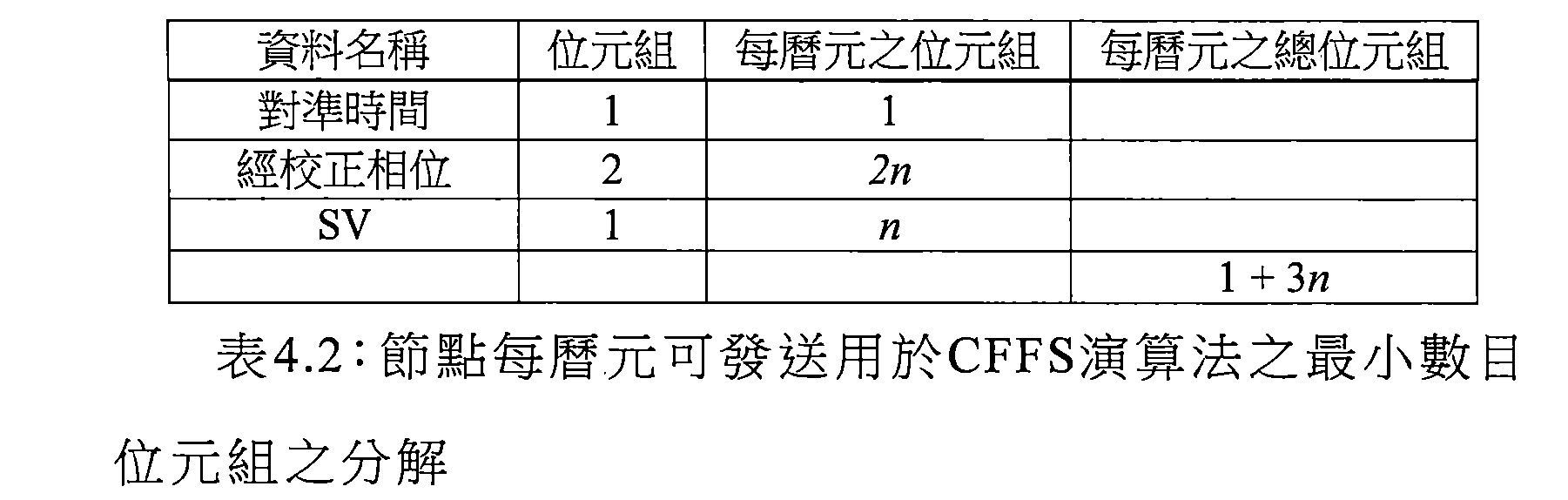
如前所述,假定一個曆元中之10個衛星的上限,此將每一節點一秒產生高達31個位元組。對於相同給定曆元速率,此等於所需要頻寬之87.5%縮減。 As mentioned earlier, assuming an upper limit of 10 satellites in an epoch, this would result in up to 31 bytes per second per node. For the same given epoch rate, this is equal to the 87.5% reduction in the required bandwidth.
4.1.1頻寬比較之真實壽命縮減4.1.1 Real life reduction of bandwidth comparison
設計及實施使用低功率無線電之藉由小太陽能面板及無電池供電的低成本GPS接收器節點。無線電鏈路並不具有封包丟失校正,封包係使用廣播方法而發送但若封包未到達,則其將不被再次發送。GPS接收器自身為單頻帶Ublox LEA6T而所使用之天線係25mm貼片及20mm螺旋天線。接收器在冬季置放在外面具有大量環繞樹及建築物之地面上。節點歸因於年時及高樹不接收直射日光。太陽 之最大仰角在正午為27°且白天長度為9.5小時。在白天之此等9.5小時期間,節點平均能夠使其GPS接收器接通大約20%時間(約一日2小時)。接收器遠離節點大約10m置放並收集資料。永久供電參考接收器用以最大化節點之重疊曆元;此置放在屋頂上。 Design and implement a low-power radio with low-cost GPS receivers and small battery-powered low-cost GPS receiver nodes. The radio link does not have packet loss correction, the packet is sent using the broadcast method but if the packet does not arrive, it will not be sent again. The GPS receiver itself is a single-band Ublox LEA6T and the antenna used is a 25mm patch and a 20mm helical antenna. The receiver is placed outside in the winter with a large number of floors surrounding the trees and buildings. The node is attributed to the year and the high tree does not receive direct sunlight. sun The maximum elevation angle is 27° at noon and 9.5 hours at daytime. During this 9.5 hour period during the day, the node is able to turn its GPS receiver on for approximately 20% of the time (about 2 hours a day). The receiver is placed approximately 10 m away from the node and collects data. The permanent power reference receiver is used to maximize the overlapping epochs of the nodes; this is placed on the roof.
進行兩個實驗,第一實驗係其中如表4.1中之全部典型資料在大約一週內傳回(「典型資料」),及另一實驗係其中係其中除了信號強度及一些除錯資訊以外的如表4.2中之來自節點演算法的輸出在大約兩週內被傳回(「節點演算法資料」)。經由無線電鏈路發送曆元丟失以及每曆元之位元組,其中比較節點傳回「節點演算法資料」情況與節點傳回「典型資料」情況;其結果係在中下表概述。 Perform two experiments. The first experimental system is that all the typical data in Table 4.1 is returned within about one week ("Typical Data"), and the other experimental system is in addition to the signal strength and some debugging information. The output from the node algorithm in Table 4.2 is passed back in approximately two weeks ("Node Algorithm Data"). The epoch loss and the octet per epoch are transmitted via the radio link, wherein the comparison node returns the "node algorithm data" status and the node returns "typical data"; the results are summarized in the following table.

與估計之87.5%相比僅僅74%資料的縮減的原因係歸因於增加之信號強度及被添加至「節點演算法資料」之除錯資訊。 The reason for the reduction of only 74% of the data compared to the estimated 87.5% is due to the increased signal strength and the debug information added to the "node algorithm data".
與正常輸出資料相比,當使用「節點演算法資料」時,存在頻寬之大約74%縮減及曆元丟失之46%縮減。因為「節點演算法資料」係來自已經由CFFS演算法部分地處理的觀測,所以資料將不能夠由典型GNSS封包使用。「節點演算法資料」為經設計用於CFFS演算法之中間資料,其為演算法自身之積分部分。 Compared with the normal output data, when using "node algorithm data", there is a reduction of about 74% of the bandwidth and a 46% reduction of the epoch loss. Since the "node algorithm data" is from observations that have been partially processed by the CFFS algorithm, the data will not be available for use by typical GNSS packets. The "node algorithm data" is an intermediate data designed for the CFFS algorithm, which is the integral part of the algorithm itself.
4.2 解比較4.2 Solution comparison
準確度及精確度可令人混淆。詳言之,準確度難以量測且藉由在每日說話中之字的共同模糊使用率使敏感之主題變得更糟。下圖展示針對藍色解集合相對於紅色真解的精確度與準確度之間的區別。黑色圓表示量測集合之精確度位準而黑色圓之中心與紅色點之中心之間的距離表示量測集合之準確度‘ Accuracy and accuracy can be confusing. In particular, accuracy is difficult to measure and makes sensitive topics worse by the common blurring of the words in everyday speech. The figure below shows the difference between the accuracy and accuracy of the blue solution set versus the red true solution. The black circle indicates the accuracy level of the measurement set and the distance between the center of the black circle and the center of the red point indicates the accuracy of the measurement set ‘

精確度可自解集合容易地估計,準確度為完全不同事項。如[48]中所指出,對於準確度而言,在內部計算並不常見,其中解係在長時間段內獲得,使得其採取正態分佈形式並假定此分佈之平均值匹配於真解。此假定並非必需有效。如吾人在多路徑章節3中看到,多路徑造成固定解偏差,即使在整日中連續採取觀測仍存在固定解偏差,且此 偏差至少在模擬中一日至下一日不改變。不可避免地系統誤差造成蠕變至解中之偏差。對於許多應用,此將並非係問題,此係因為無論如何皆不改變的固定偏差僅意謂你始終量測你的設備之不同點。然而,多路徑引起方位相依偏差,若GPS接收器移動,則此偏差相對於解之平均位置改變,因此使在足夠大時段內採取的正態分佈解之平均值匹配於真解的假定無效。量測真實位置需要外部計算準確度,此意謂使用具有較好準確度之某一其他裝置。此超出此論文之範疇,因此吾人僅僅考慮近似內部準確度評估。如[48]所說,「記住任何給定GPS量測可由以下方程式表示:量測=確切值+偏差+隨機誤差。隨機誤差分量呈現針對內部及外部評估兩者之大致相同問題。然而,偏差需要用於偵測之外部真值。不存在藉由僅僅研究經移位資料集自資料集中之真值偵測恆定移位之容易方式。」。 Accuracy can be easily estimated from the set of solutions, and the accuracy is completely different. As noted in [48], internal calculations are not common for accuracy, where the solution is obtained over a long period of time such that it takes a normal distribution and assumes that the mean of this distribution matches the true solution. This assumption is not required to be valid. As we saw in multipath chapter 3, multipath causes a fixed solution deviation, even if continuous observations are taken throughout the day, there is still a fixed solution deviation, and this The deviation does not change at least in the simulation from one day to the next. Inevitably the systematic error causes creep to the deviation in the solution. For many applications, this will not be a problem, because the fixed deviation that does not change anyway simply means that you always measure the difference between your device. However, multipath causes azimuth dependent deviation, and if the GPS receiver moves, the deviation changes relative to the average position of the solution, thus invalidating the assumption that the average of the normal distribution solutions taken over a sufficiently large period of time matches the true solution. Measuring the real position requires external calculation accuracy, which means using some other device with better accuracy. This is beyond the scope of this paper, so we only consider the approximate internal accuracy assessment. As noted in [48], "Remember that any given GPS measurement can be represented by the following equation: measurement = exact value + deviation + random error. The random error component presents roughly the same problem for both internal and external evaluations. However, The deviation needs to be used for the detection of the external truth value. There is no easy way to detect a constant shift from the true value of the data set by shifting the data set.".
雖然很可能難以量測,歸因於多路徑引起的偏差,但運用高品質GPS天線在低多路徑環境中使用24小時觀測最可能產生部分歸因於環境及裝備,及亦部分歸因於獲得瞬時多路徑偏差之平均值的24小時觀測的小偏差。在此狀況下,內部獲得準確度很可能相當接近於實際準確度。然而,對於吾人之應用,吾人具有不具有扼流環之不良未經校準之天線、高多路徑環境,及歸因於多路徑且僅僅能夠獲得白天時間觀測所造成的偏差之每年預測之循環。此意謂可靠地內部計算準確度係非常困難且潛在地更不準確。如第3章預測的每年解偏差循環特別地使準確度估計非常困難, 此係因為將需要至少一年有價值觀測來考慮每年解偏差循環。 Although it is likely to be difficult to measure due to multipath-induced deviations, the use of high-quality GPS antennas in low-multipath environments using 24-hour observations is most likely due in part to the environment and equipment, and partly due to A small deviation of the 24-hour observation of the average of the instantaneous multipath deviations. In this case, the internal accuracy is likely to be quite close to the actual accuracy. However, for our application, we have a bad uncalibrated antenna without a choke, a high multipath environment, and an annual forecast cycle due to multipath and only being able to obtain deviations from daytime observations. This means that reliable internal computational accuracy is very difficult and potentially less accurate. The annual solution deviation cycle as predicted in Chapter 3 makes it very difficult to estimate the accuracy, This is because the annual de-bias cycle is considered for at least one year of valuable observations.
在無某一類型量測之情況下,準確度及精確度係無意義的。準確度及精確度量測通常係解將在某一給定大小之某一形狀內的機率。一般而言,所使用形狀係圓或球體且概率自50%向上。2D水平(北東向)似乎係很可能最常給予的,此係因為與向上方向相比,GPS解在此平面中往往會更精確,且在此平面中相當地對稱。下表定義三個非常常見量測,其中CEP DRMS及2DRMS係針對2D水平面且SEP係針對全部三個維度。對於一個維度,通常使用向上方向RMS。 In the absence of a certain type of measurement, accuracy and precision are meaningless. Accuracy and accurate metrology typically resolve the probability of being within a certain shape of a given size. In general, the shape used is a circle or sphere with a probability from 50% up. The 2D level (north-east) seems to be most likely to be given most often because the GPS solution tends to be more accurate in this plane than in the upward direction and is quite symmetrical in this plane. The table below defines three very common measurements, where CEP DRMS and 2DRMS are for the 2D horizontal plane and the SEP is for all three dimensions. For a dimension, the upward direction RMS is usually used.

下表展示吾人用以計算此等量測的近似計算,其中σ N 、σ E 及σ U 分別為在北東及向上方向中的解之標準差。此等公式係自[26]獲得。 The following table shows the approximate calculations that we use to calculate these measurements, where σ N , σ E , and σ U are the standard deviations of the solutions in the northeast and upward directions, respectively. These formulas are obtained from [26].

吾人在此論文中僅僅考慮內部準確度且當吾人討論解之準確度時,吾人意謂吾人已自充分大數量的解之樣本獲得群體之標準差的估計,吾人希望此等解之平均值與真解相同且已計算如前一表中之準確度。對於解精確度,當吾人通常處理每天解且僅僅能夠一日計算一解時,解之精確度意謂如當解之低頻分量已被移除從而僅留下高頻分量時使用在不大於幾個月之一時間段內或在更長時間段內採取的解集自前一表所量測之精確度。 In this paper, we only consider internal accuracy and when we discuss the accuracy of the solution, we mean that we have obtained an estimate of the standard deviation of the group from a sample of a sufficient number of solutions. We hope that the average of these solutions The true solution is the same and the accuracy as in the previous table has been calculated. For solution accuracy, when we usually deal with daily solutions and can only calculate one solution per day, the accuracy of the solution means that if the low-frequency component of the solution has been removed and only the high-frequency component is left, it is used in no more than a few. The accuracy of the solution taken from the previous table during the period of one month or for a longer period of time.
4.2.1比較方法4.2.1 Comparison method
吾人設計被稱為JAC-MM及JAC之兩個程式。JAC-MM實施CFFS演算法,而JAC實施除了恆星濾波階段以外的CFFS演算法。若吾人假定遠端GNSS接收器設置與電力網隔離並經由無線鏈路連接至使用者,則若吾人縮減硬體及部署之成本及功率要求,則使用者將最可能獲得較少類型之觀測,或多或少間歇觀測,增加之多路徑,增加之PCV,及大體上較不良品質資料。接著繼續存在的問題係有可能仍獲得準確/精確靜態解且若如此則該等準確/精確靜態解之準確/精確程度很可能將如何。就此而言,吾人將不預期當前GNSS軟體進行特別好的工作,此係因為設計軟體之人可能假定可得到連續高品質資料。因此,吾人經由JAC及JAC-MM運行不同類型修改之觀測並比較此等靜態相關解與經由開放源GNSS套件RTKLib[11]及GPSTk[8]運行的相同修改之觀測。使用RTKLib及GPSTk,此係因為此等係支援吾人發現的基於單頻帶相位之相對方位解的可免費得 到之僅有兩個開放源GNSS套件。日復一日地獲得靜態解。 I designed two programs called JAC-MM and JAC. JAC-MM implements the CFFS algorithm, while JAC implements the CFFS algorithm in addition to the stellar filtering stage. If we assume that the remote GNSS receiver settings are isolated from the power grid and connected to the user via a wireless link, then if we reduce the cost and power requirements of the hardware and deployment, the user will most likely receive fewer types of observations, or More or less intermittent observations, increased multipath, increased PCV, and generally poorer quality data. It is then possible to continue to have an accurate/accurate static solution and if so, how accurate/accurate the exact/precise static solution is likely to be. In this regard, we will not expect the current GNSS software to perform particularly well, because the person designing the software may assume that continuous high quality data is available. Therefore, we run different types of modified observations via JAC and JAC-MM and compare the observations of these static correlation solutions with the same modifications run via the open source GNSS suites RTKLib [11] and GPSTk [8]. Using RTKLib and GPSTk, because this system supports the relative orientation solution based on single-band phase that we found, it is free. There are only two open source GNSS kits. Get a static solution day after day.
除了多種其他解類型(諸如RTK、精確點定位(PPP)、差分GPS(DGPS)、單一、固定等)以外,RTKLib亦進行靜態解。支援單頻帶及雙頻帶接收器兩者。對於在小於10km之短暫基線上的靜態解,使用某一形式之擴展卡爾曼濾波器及雙差[52](第161頁)。 In addition to a variety of other solution types (such as RTK, precise point positioning (PPP), differential GPS (DGPS), single, fixed, etc.), RTKLib also performs static solutions. Both single-band and dual-band receivers are supported. For static solutions over short baselines of less than 10 km, some form of extended Kalman filter and double difference [52] (page 161) are used.
GPSTk其中具有稱為DDBase之能夠使用僅僅單頻接收器計算靜態解及亦使用雙差的應用程式[35]。 GPSTk has an application called DDBase that can calculate static solutions using only single-frequency receivers and also uses double difference [35].
JAC實施CFFS演算法但在不運用恆星濾波。因此,JAC計算之全部每天解僅基於在正如RTKLib及GPSTk所在之彼日內獲得的觀測。此允許三個程式之間的有意義之效能比較。 JAC implements the CFFS algorithm but does not use stellar filtering. Therefore, all of the daily solutions for JAC calculations are based only on observations taken within the same day as RTKLib and GPSTk. This allows for a meaningful performance comparison between the three programs.
恆星濾波使用來自先前日之資訊以計算解且因此與JAC GPSTk及RTKLib作比較並不公平。恆星濾波演算法可附加至此等三個程式中之任一者以獲得較高準確度/精確度之解。然而,吾人將恆星濾波之實施方案附加至JAC程式,以便看到恆星濾波與其他三個程式相比具有的效應;具有附加恆星濾波之此JAC程式稱為JAC-MM且為如第2章中所描述的吾人之CFFS演算法的完整實施方案。 Stellar filtering uses information from previous days to calculate solutions and is therefore unfair compared to JAC GPSTk and RTKLib. A stellar filtering algorithm can be attached to any of these three programs to obtain a higher accuracy/accuracy solution. However, we have attached the implementation of the stellar filter to the JAC program to see the effects of stellar filtering compared to the other three programs; this JAC program with additional stellar filtering is called JAC-MM and is as in Chapter 2 A complete implementation of the CFFS algorithm described by us.
4.2.2連續高品質資料4.2.2 Continuous high quality data
此子章節之目標係展示CFFS演算法的吾人實施方案產生與在良好品質條件下之預先存在解處理程式相當的解。對於最初效能測試,吾人使用自GPS接收器獲得之兩月高品質資料,第一GPS接收器定位在Te Papa博物館且第 二GPS接收器定位在惠靈頓機場。此資料係自陸地及資訊紐西蘭(LINZ)之RINEX資料存檔獲得[5]。資料速率為每30秒一個曆元。此等兩個接收器之間的基準為約4km。兩個接收器為Trimble NetRS[12]而天線係不同的,一者為LEIAT504且另一者為TRM41249.00。資料藉由GeoNet計劃供應至吾人。接收器及天線之此等類型為高端雙頻帶。如藉由資料表給出的此接收器之靜態解準確度針對水平方向為5mm+0.5ppmDRMS,且針對向上方向為5mm+1ppm RMS,其中ppm係指基準長度。此意謂資料表暗示如藉由接收器自身計算之靜態解針對水平將為14mm 2DRMS。功率消耗係介於3W與4W之間。 The goal of this subsection is to show that the implementation of the CFFS algorithm produces a solution that is comparable to a pre-existing solution in good quality conditions. For the initial performance test, we used two months of high quality data obtained from a GPS receiver, the first GPS receiver positioned at the Te Papa Museum and the second GPS receiver positioned at Wellington Airport. This information was obtained from the RINEX data archive of Land and Information New Zealand (LINZ) [5]. The data rate is one epoch every 30 seconds. The reference between these two receivers is approximately 4 km. The two receivers are Trimble NetRS [12] and the antenna system is different, one is LEIAT504 and the other is TRM41249.00. The information is supplied to us through the GeoNet program. These types of receivers and antennas are high-end dual bands. The static solution accuracy of this receiver as given by the data sheet is 5 mm + 0.5 ppm DRMS for the horizontal direction and 5 mm +1 ppm RMS for the upward direction, where ppm is the reference length. This means that the data sheet implies that the static solution, as calculated by the receiver itself, will be 14 mm 2DRMS for the level. The power consumption is between 3W and 4W.
為了公平比較,當吾人之演算法意欲僅僅處理單頻帶GPS接收器時,首先藉由剝除精確P代碼以及L2頻帶觀測而修改觀測,以便僅留有C1、D1、S1及L1觀測類型及廣播導航資料;此等類型觀測對於低成本低功率單頻帶GPS接收器係典型的。 For fair comparison, when our algorithm is intended to process only single-band GPS receivers, the observations are first modified by stripping the exact P code and the L2 band observations so that only the C1, D1, S1, and L1 observation types and broadcasts are left. Navigation data; these types of observations are typical for low cost, low power single band GPS receiver systems.
DDBase歸因於不能夠正確地讀取導航檔案而在第六天失效,而不管此等檔案係自IGS產品獲得[27]。GPSTk及JAC兩者獲得全部天之解以供處理。圖4.2展示解之鳥眼視圖而表4.6展示解之一些統計,其中NEU為北東上之縮寫。亦包括JAC-MM解。 DDBase expired on the sixth day due to failure to properly read the navigation file, regardless of whether the files were obtained from IGS products [27]. Both GPSTk and JAC get all the solutions for processing. Figure 4.2 shows the bird's eye view of the solution and Table 4.6 shows some statistics of the solution, where NEU is the abbreviation of North East . Also includes the JAC-MM solution.
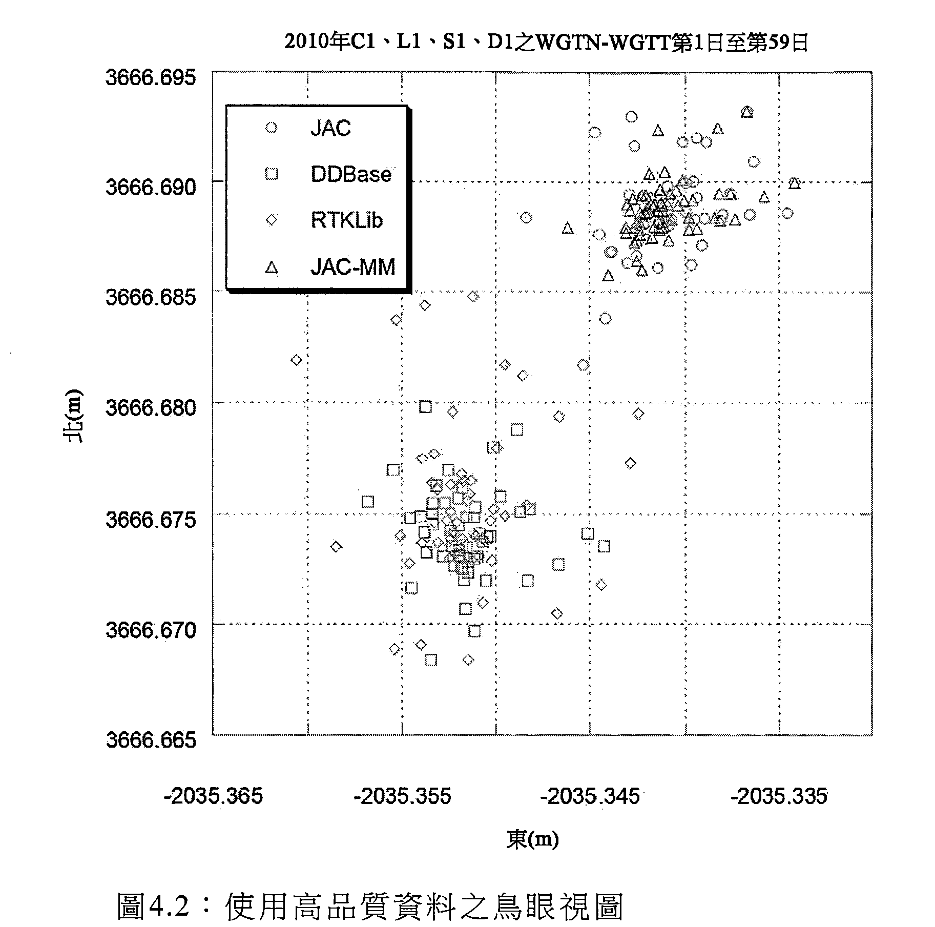

如可看到,全部程式產生具有相當精確度之解全部解之標準差類似。在水平面中,DDBase及RTKLib彼此平均起來在一毫米內一致,在垂直方向中RTKLib高於DDBase 1.6cm。JAC在垂直方向中與DDBase在8mm內一致而在水平面中,JAC不同於DDBase及RTKLib兩者大約1.8cm。JAC與DDBase差為20mm,JAC與RTKLib差為20mm且DDBase 與RTKLib差為16mm。準確度之三個量測係在下表中概述。 As can be seen, the standard deviation of all solutions yielding a solution with comparable accuracy is similar. In the horizontal plane, DDBase and RTKLib are averaged within one millimeter of each other, and RTKLib is 1.6 cm higher than DDBase in the vertical direction. JAC is consistent with DDBase within 8 mm in the vertical direction and in the horizontal plane, JAC is approximately 1.8 cm different from both DDBase and RTKLib. The difference between JAC and DDBase is 20mm, the difference between JAC and RTKLib is 20mm and DDBase The difference from RTKLib is 16mm. The three measurements of accuracy are summarized in the table below.

如已提及,JAC-MM使用來自先前日之資料計算解。因此,當直接與其他三個程式解相比時,JAC-MM解之結果係不公平的。然而,如所預期,JAC-MM之解比其他三個程式更精確。亦引起關注的係應注意,恆星濾波改良精確度而不管觀測僅僅具有每30秒一次之曆元速率。此係引起關注的,由於所需要的恆星移位意謂今天不存在如昨天存在的一對衛星之匹配觀測,此係因為246/30並非為整數。實際上,花費五天間隔出現一對衛星之匹配觀測。檢查數目,對於此資料,JAC-MM比JAC約多20%精確度。 As already mentioned, JAC-MM uses the data from previous days to calculate the solution. Therefore, the results of the JAC-MM solution are unfair when compared directly to the other three program solutions. However, as expected, the JAC-MM solution is more accurate than the other three programs. It is also interesting to note that stellar filtering improves accuracy regardless of whether the observation has only an epoch rate once every 30 seconds. This is of concern, since the required star shift means that there is no matching observation of a pair of satellites that existed yesterday, because 246/30 is not an integer. In fact, a pair of satellite matching observations occurred at five-day intervals. The number of inspections, for this information, JAC-MM is about 20% more accurate than JAC.
當彼此比較時,全部程式具有範圍介於16mm至20mm之顯著解偏差。出於吾人之目的,吾人不關注不隨位置或隨著時間而改變的解偏差。使用三個不同程式造成的此等偏差是否隨位置或擴展時間改變,吾人不知曉。下圖展示在值得處理之此等兩個月內具有95%可信度球體之平均解。如可看到,其中無一者彼此一致。JAC-MM之球體並未標繪為在JAC之球體內。引起關注的係應注意,全部程式使用相同觀測但全部程式產生不同結果。全部程式產生非常精確結果。 When compared to each other, all programs have significant solution deviations ranging from 16 mm to 20 mm. For my purposes, we do not care about deviations that do not change with location or over time. Whether these deviations caused by using three different programs change with position or expansion time, I don't know. The figure below shows the average solution with a 95% confidence sphere for the two months worth dealing with. As can be seen, none of them are consistent with each other. The sphere of JAC-MM is not plotted as being in the sphere of JAC. Attention should be paid to the fact that all programs use the same observations but all programs produce different results. All programs produce very accurate results.

4.2.3模擬間歇高品質資料4.2.3 Simulating intermittent high quality data
藉由使用如前所述之相同高品質Te Papa惠靈頓機場資料(但其中隨機地移除衛星觀測之50%)建立模擬間歇高品質資料。如前所述,經由JAC、DDBase及RTKLib運行資料。DDBase及RTKLib未能傳回任何解。圖4.4展示解之鳥眼視圖而表4.8展示解之一些統計且表4.9展示解之精確度的量測。 Simulated intermittent high quality data was created by using the same high quality Te Papa Wellington airport data as previously described (but randomly removing 50% of satellite observations). As mentioned earlier, the data is run via JAC, DDBase and RTKLib. DDBase and RTKLib failed to return any solution. Figure 4.4 shows the bird's eye view of the solution and Table 4.8 shows some statistics for the solution and Table 4.9 shows the measurement of the accuracy of the solution.
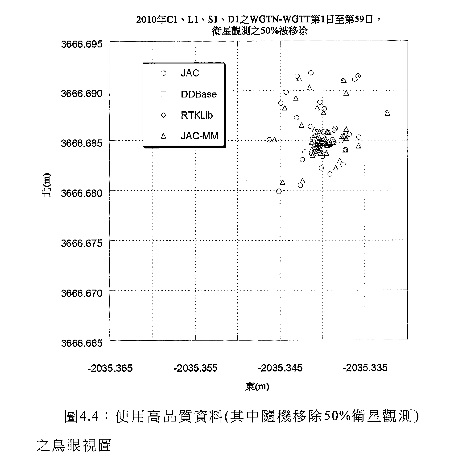
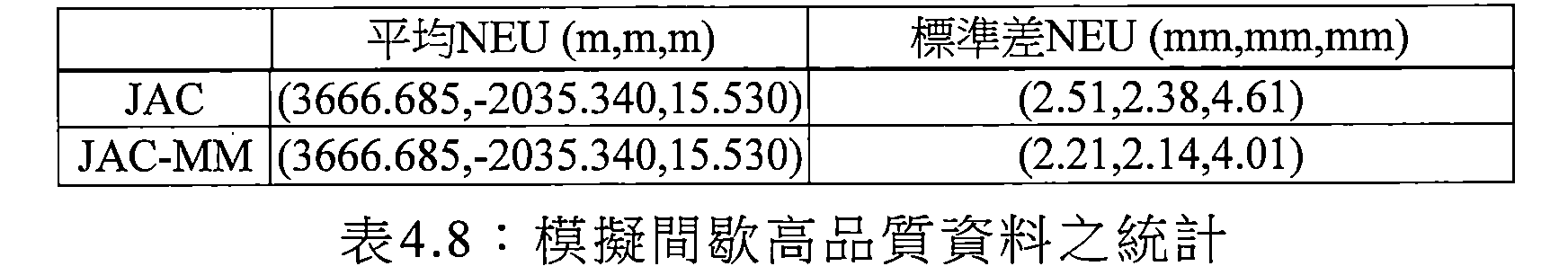
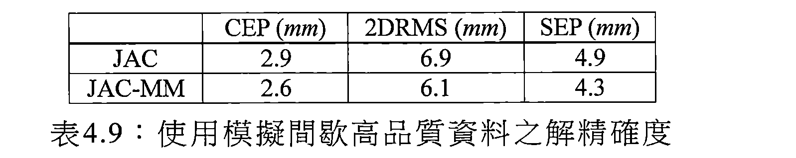
JAC之解幾乎與之前其中未移除衛星觀測之情境相同;平均位置為兩者之間的4mm差。如可看到,有效隨機地移除50%衛星觀測使JAC之解的精確度有極少差。 The JAC solution is almost identical to the previous scenario in which satellite observations were not removed; the average position is 4 mm difference between the two. As can be seen, the effective and random removal of 50% of satellite observations results in very little accuracy in the JAC solution.
4.2.4使用真實壽命間歇不良品質資料之演算法效能4.2.4 Algorithm performance using real life intermittent bad quality data
此子章節之目標為判定三個程式(JAC、DDBase及RTKLib)中之任一者是否可使用自吾人設計之GPS WSN節點獲得的真實壽命間歇不良品質資料獲得合理精確度之解。用以獲得曆元丟失之子章節4.1.1中使用的相同兩個實驗亦用以獲得真實壽命間歇不良品質資料。 The goal of this subsection is to determine whether any of the three programs (JAC, DDBase, and RTKLib) can use the true lifetime misperformed quality data obtained from the GPS WSN node designed by us to obtain a reasonable accuracy solution. The same two experiments used in subsection 4.1.1 to obtain epoch loss are also used to obtain real life intermittent bad quality data.
CFFS演算法經設計為分佈式演算法,其中演算法中之一些係在節點自身上運行。此具有如子章節4.1.1中所看到之曆元丟失縮減的優點。在不考慮此之情況下比較CFFS演算法與DDBase及RTKLib將係不公平的。若節點僅傳回「典型資料」且CFFS演算法之節點區段將以非分佈式方式在基地台上運行,則與如表4.3中所看到之14%曆元丟失相比,CFFS演算法可帶來26%曆元丟失。因此,兩個節點設置經組配。藉由節點傳回「典型資料」的第一設置,及藉由節點傳回「節點演算法資料」的另一設置。第一設置經設計以將資料供應至DDBase及RTKLib,而第二設置經設計以將資料供應至CFFS演算法之主要部分。 The CFFS algorithm is designed as a distributed algorithm in which some of the algorithms run on the nodes themselves. This has the advantage of epoch loss reduction as seen in subsection 4.1.1. It is unfair to compare CFFS algorithms with DDBase and RTKLib without considering this. If the node only returns "typical data" and the node segment of the CFFS algorithm will run on the base station in a non-distributed manner, the CFFS algorithm is compared to the 14% epoch loss as seen in Table 4.3. Can bring 26% epoch lost. Therefore, the two node settings are assembled. The node returns the first setting of "Typical Data" and returns another setting of "Node Algorithm Data" by the node. The first setting is designed to supply data to DDBase and RTKLib, while the second setting is designed to supply data to the main part of the CFFS algorithm.
大約1週之「典型資料」經獲得用於DDBase及RTKLib,而大約2週之「節點演算法資料」經獲得用於CFFS演算法之主要部分以待處理。觀測並非同時採取,且歸因於需要再程式化節點以輸出「節點演算法資料」而非「典型資料」,其中節點之位置在兩個資料收集時段期間不可避免地稍微移位。此等移動係極小的且不改變吾人之結果。下圖展示解結果之鳥眼視圖。JAC計算全部日之解。 DDBase可計算全部日之解但其係不準確的,RTKLib並不成功地計算任何解。 About 1 week of "typical data" was obtained for DDBase and RTKLib, and about 2 weeks of "node algorithm data" was obtained for the main part of the CFFS algorithm for processing. The observations are not taken at the same time, and due to the need to reprogram the nodes to output "node algorithm data" rather than "typical data", where the position of the nodes is inevitably slightly shifted during the two data collection periods. These movements are extremely small and do not change the results of our people. The figure below shows the bird's eye view of the solution. JAC calculates the solution for all days. DDBase can calculate all day solutions but its system is not accurate. RTKLib does not successfully calculate any solution.

為了比較對歸因於當使用JAC時在基地台中之節點之間傳輸「節點演算法資料」(而非「典型資料」)時曆元丟失之縮減而獲得解之能力的影響,節點演算法實施於基地台上且DDBase及RTKLib的用以計算以上解的一週有價值資料經由JAC而運行。JAC計算全部日之解;所獲得解之鳥眼視圖在下圖中展示。 In order to compare the impact of the ability to obtain solutions due to the reduction of epoch loss when transmitting "node algorithm data" (rather than "typical data") between nodes in the base station when using JAC, node algorithm implementation The one-week valuable data used to calculate the above solution on the base station and DDBase and RTKLib is run via JAC. JAC calculates the solution for all days; the bird's eye view of the solution is shown in the figure below.
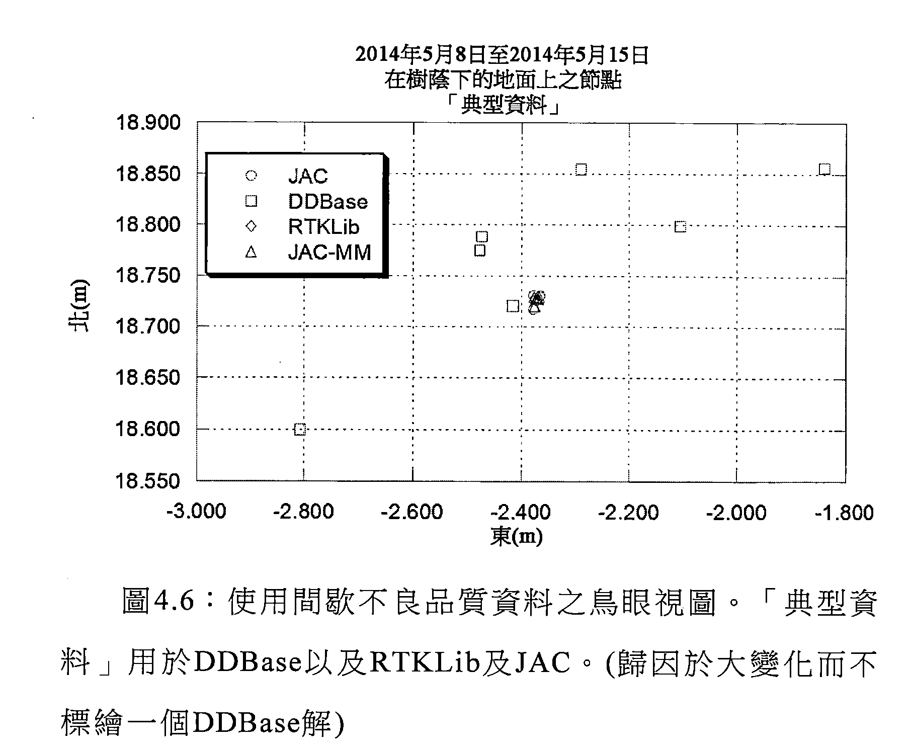
如可看到,不管曆元丟失之增加,JAC非常類似於在節點與基地台之間傳輸「節點演算法資料」的情況而進行。以下兩個表概述解之一些統計。 As can be seen, regardless of the increase in epoch loss, JAC is very similar to the case where "node algorithm data" is transmitted between the node and the base station. The following two tables summarize some of the statistics of the solution.
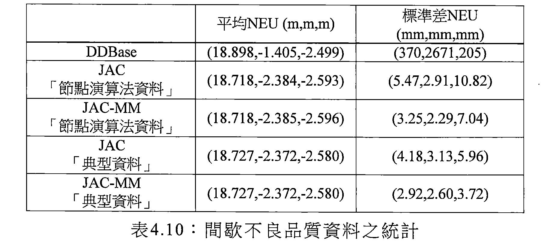

如可看到,僅僅JAC能夠獲得任一真實值之解。JAC之精確度的量測為高品質Te Papa惠靈頓機場資料之精確度量測的大約雙倍。歸因於小樣本大小,相比於「節點演算法資料」,當傳輸「典型資料」時JAC之樣本標準差不同於吾人將預期的標準差。與當傳輸「節點演算法資料」時相比,當在節點與基地台之間傳輸「典型資料」時引發的較高曆元丟失對能夠獲得有效解沒有顯著的效應。 As can be seen, only JAC can get a solution of any real value. The accuracy of the JAC is approximately doubled for the accurate measurement of the high quality Te Papa Wellington airport data. Due to the small sample size, the sample standard deviation of JAC is different from the standard deviation that we would expect when transmitting "typical data" compared to "node algorithm data". The higher epoch loss caused when transmitting "typical data" between a node and a base station has no significant effect on the ability to obtain an effective solution compared to when transmitting "node algorithm data".
4.2.5解比較概述4.2.5 Overview of the solution
在下圖中描繪定性概述。 A qualitative overview is depicted in the figure below.
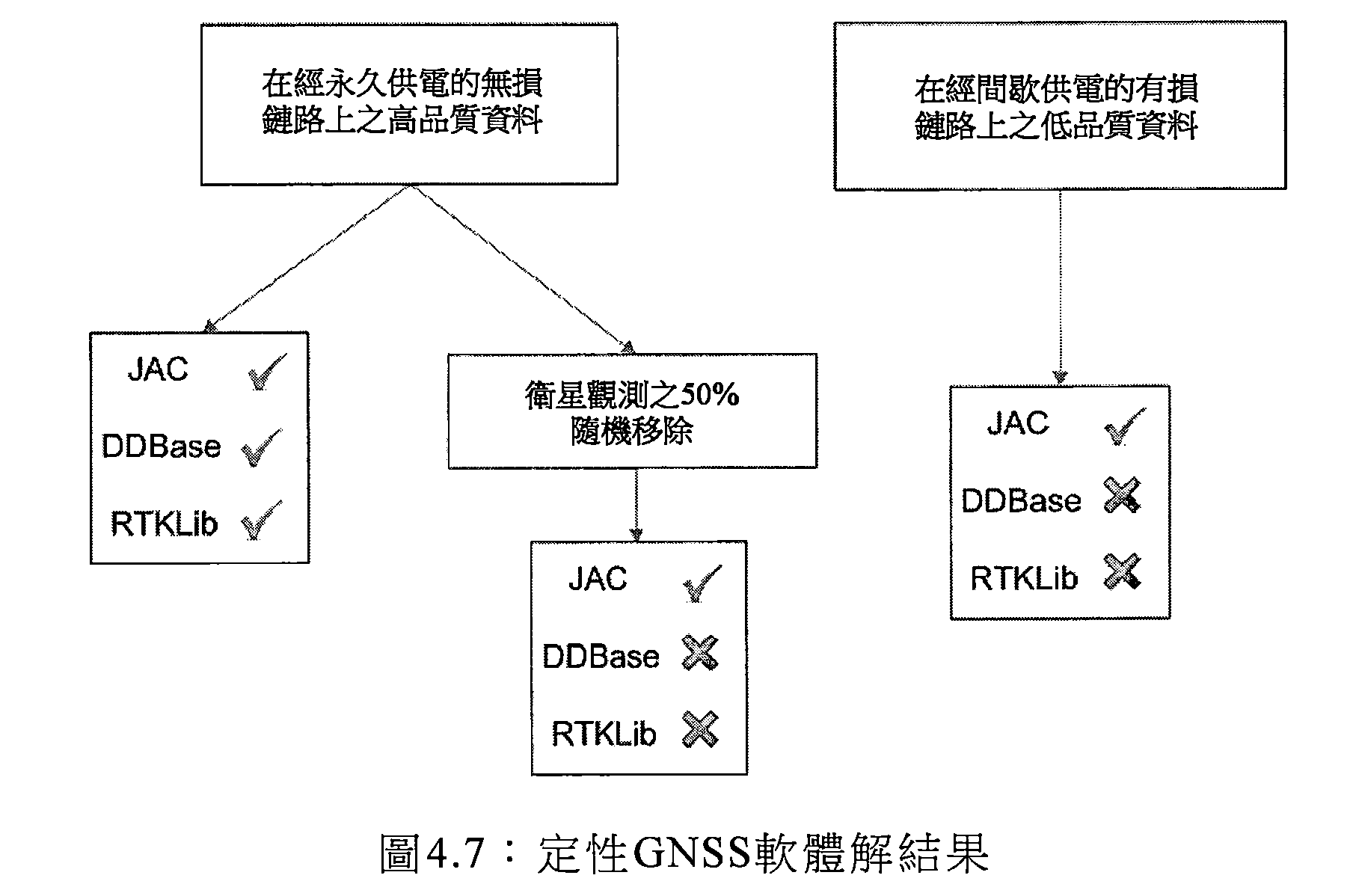
全部三個程式在使用經由經永久供電的無損無線電鏈路之高品質GPS資料時獲得類似的精確度,而同時產生相對於彼此範圍介於16mm至20mm之顯著不同偏差。DDBase及RTKLib兩者對遺漏衛星觀測極敏感而JAC對此等事件不敏感。歸因於JAC之對遺漏衛星觀測的不敏感度 及小樣本大小,相比於傳輸「典型資料」,當傳輸「節點演算法資料」時偵測精確度之不顯著改良。如所預期,與當在低多路徑環境中使用高端裝備時相比,當在高多路徑環境中使用吾人之低端硬體時JAC之解更糟。當使用吾人之GPS WSN節點時,僅僅JAC及JAC-MM可產生任何有意義準確度之解。因此,當JAC-MM為吾人之CFFS演算法的實施方案時,CFFS演算法適合於使用吾人之硬體的地面變形監測的吾人之應用。 All three programs achieve similar accuracy when using high quality GPS data via permanently powered lossless radio links, while at the same time producing significantly different deviations ranging from 16 mm to 20 mm with respect to each other. Both DDBase and RTKLib are extremely sensitive to missing satellite observations and JAC is not sensitive to such events. Attributable to JAC's insensitivity to missing satellite observations And the small sample size, compared to the transmission of "typical data", the detection accuracy is not significantly improved when transmitting "node algorithm data". As expected, the JAC solution is even worse when using our low-end hardware in a high multipath environment compared to when using high-end equipment in a low multipath environment. When using our GPS WSN node, only JAC and JAC-MM can produce any meaningful accuracy solution. Therefore, when JAC-MM is an implementation of our CFFS algorithm, the CFFS algorithm is suitable for our application using ground deformation monitoring of our hardware.
雖然準確度可並不完全知曉,但歸因於吾人系統之高精確度可量測僅幾個公釐之小急劇移動。 Although the accuracy may not be fully known, due to the high accuracy of our system, only a few millimeters of sharp movement can be measured.
試驗台結果及分析Test bench results and analysis
6.1 Paekakariki試驗台6.1 Paekakariki test bench
在下圖中展示Paekakariki試驗台。如由紫色圓描繪,節點彼此相對接近而置放·另外,永久供電GPS接收器節點置放在圖之右下手拐角處的建構之屋頂上。圖之左邊為北方向。 The Paekakariki test rig is shown in the image below. As depicted by the purple circle, the nodes are placed relatively close to each other. Additionally, the permanently powered GPS receiver node is placed on the constructed roof at the right lower hand corner of the figure. The left side of the figure is the north direction.
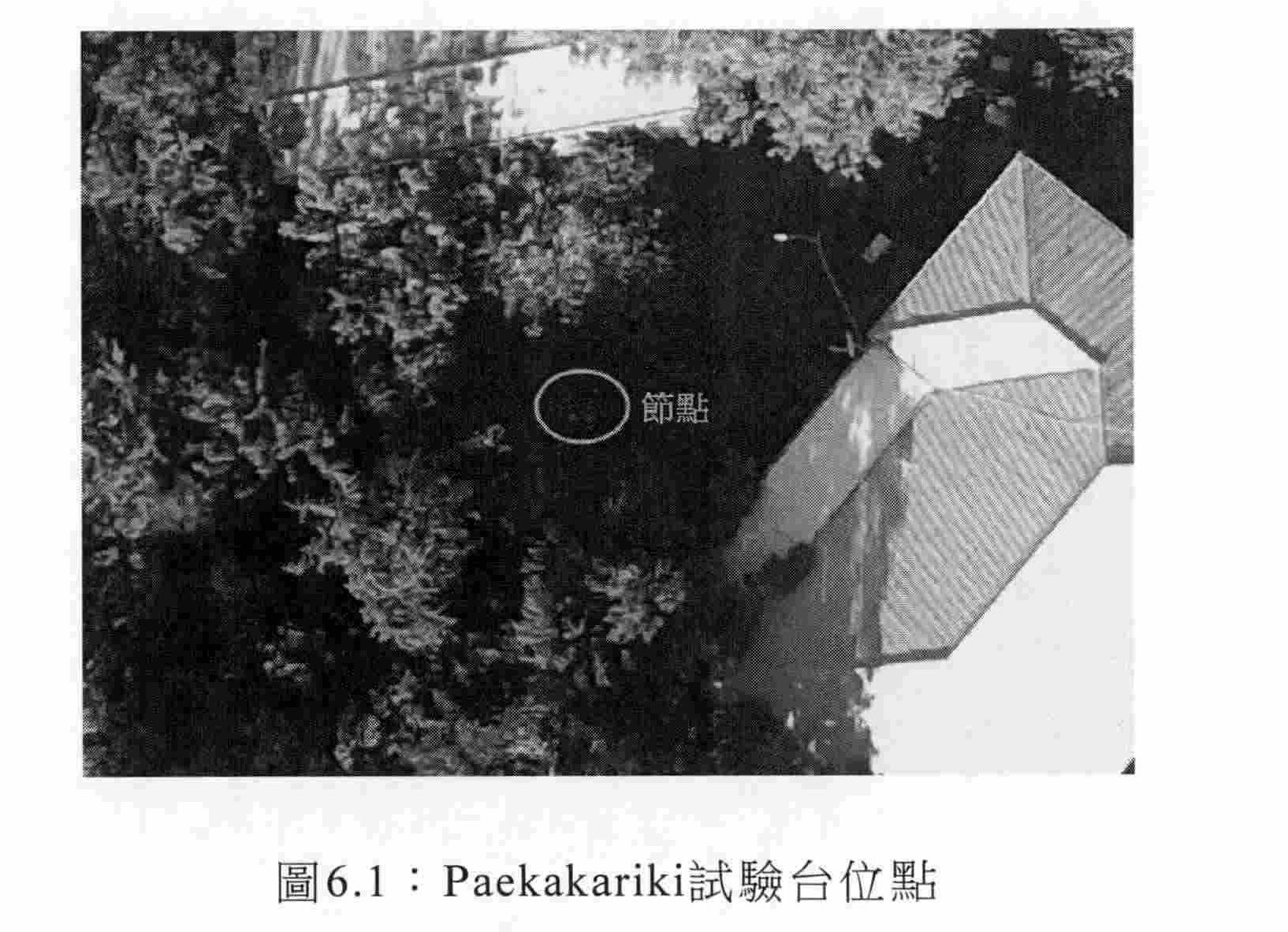
如可看到,用於地面上之節點之Paekakariki試驗台存在不良天空可見度,而在屋頂上之接收器具有稍微較好可見度。在此論文全篇中使用自此試驗台獲得之觀測及使用其之結果。 As can be seen, the Paekakariki test rig for nodes on the ground has poor sky visibility, while the receiver on the roof has slightly better visibility. The observations obtained from this test bed and the results of their use are used throughout this paper.
首先,吾人研究GPS接收器在一日中往往會在作用中的小時之數目及此數目如何變化。下圖展示節點272之GPS當在夏季及接著在冬季持續大約兩週置放於Paekakariki測 試位點處時每日在作用中及成功地傳回曆元的小時之數目。 First, we study the number of hours that a GPS receiver tends to be active in a day and how this number changes. The figure below shows that the GPS of node 272 is placed in Paekakariki during the summer and then in the winter for about two weeks. The number of hours in the active and successful return of the epoch at the test site.

在冬季,吾人觀測最小小於0.5小時,而在夏季吾人觀測最大大於8小時。平均起來,在冬季存在1.7小時在作用中而在夏季存在6.2小時在作用中;與冬季解相比,此意謂3.6倍多的曆元用於處理夏季解。下圖中描繪使用JAC-MM實施CFFS演算法之水平解。 In the winter, we observed a minimum of less than 0.5 hours, while in the summer we observed a maximum of more than 8 hours. On average, there are 1.7 hours in effect in winter and 6.2 hours in summer; this means that 3.6 times more epochs are used to process summer solutions than in winter solutions. The horizontal solution using the JAC-MM to implement the CFFS algorithm is depicted in the following figure.

如可看到,與冬季相比,似乎在夏季期間有更好精確度,如吾人預期,與冬季解相比,存在3.6倍多的曆元用於夏季解。 As can be seen, it seems that there is better precision during the summer than in winter. As I expected, there are 3.6 times more epochs for the summer solution than the winter solution.
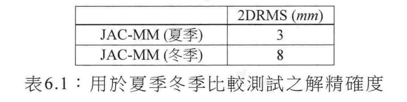
以下圖像展示在夏季持續一個月運行的在Paekakariki試驗台位點處之部署,其中北係在圖像之向上方向中且節點直接置放在地面上;此等三個節點可正好在圖6.1中看到。如此圖中可看到,樹陰影經過該等節點。 The following image shows the deployment at the Paekakariki test rig site, which lasts for one month in the summer, where the North is in the upward direction of the image and the nodes are placed directly on the ground; these three nodes can be exactly in Figure 6.1. Seen in. As you can see in the figure, the tree shadow passes through the nodes.

使用具有大約1cm之準確度的卷尺來量測至天線中的每一者之近似實體水平中心的量測。以下圖中描繪此等量測之結果。 A tape measure having an accuracy of about 1 cm is used to measure the measurement of the approximate physical horizontal center to each of the antennas. The results of these measurements are depicted in the following figures.
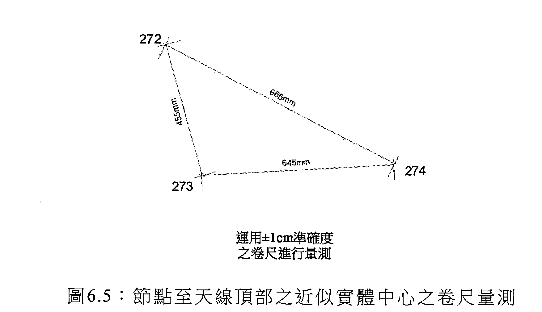
在一個月之後處理每天解,且在下圖中標繪全部水平解;每一節點之間的平均距離亦以如自CFFS解之水平分量導出的95%不確定度在以下圖中描繪。 The daily solution is processed after one month, and all horizontal solutions are plotted in the following figure; the average distance between each node is also depicted in the following figure as 95% uncertainty derived from the horizontal component of the CFFS solution.

因為三個天線中之每一者的相位中心(由於其為未經校準之天線)尚未知曉,所以對於使用卷尺的天線之近似實 體中心之間的相對距離量測之間的差,及水平CFFS解之平均值之間的差,吾人應預期此等僅僅為近似值。然而,不管此,此等距離值之差仍與使用卷尺量測的差一致。 Since the phase center of each of the three antennas (because it is an uncalibrated antenna) is not known, the approximate implementation of the antenna using the tape measure The difference between the relative distance measurements between the center of the body and the difference between the average of the horizontal CFFS solutions, which we should expect, are only approximations. However, regardless of this, the difference between these equidistance values is still consistent with the difference in the measurement using the tape measure.
持續此一個月靜態測試對於三個節點計算的平均2DRMS精確度為5mm且似乎為對於高多路徑環境之解精確度的典型值。 The one-month static test lasted for the three nodes calculated with an average 2D RMS accuracy of 5 mm and appears to be a typical value for the solution accuracy of the high multipath environment.
6.2 廬山試驗台6.2 Lushan Test Bench
廬山位點為在臺灣南投山區的高於廬山之城鎮之坡道上的已知高危地滑位點。其為使用衛星成像、空中成像、雷射器測量及GPS研究的位點。作用中移動區帶大約涵蓋1km2且類似於在坡道之頂部開始的倒V之形狀。 The Lushan site is a known high-risk ground-slip site on the slope of the town of Nantou, Taiwan, which is higher than the town of Lushan. It is a site for satellite imaging, aerial imaging, laser measurement, and GPS research. The active zone is approximately 1 km 2 in length and resembles the shape of the inverted V starting at the top of the ramp.
4個小無電池GPS無線感測器節點之試驗台經部署於該位點處。節點係使用國立暨南國際大學(NCNU)之總台沿著用於基於雷射之地面變形監測之逆向反射器的邊而部署。 A test bed of four small batteryless GPS wireless sensor nodes is deployed at the site. The node system is deployed using the main station of the National University of South China (NCNU) along the side of the retroreflector for laser based ground deformation monitoring.
歸因於密集且高的植被,網路涵蓋及GPS衛星之充分可見度兩者係有問題的。為了充分網路涵蓋,使用兩個無電池太陽能供電無線電中繼器。一個中繼器置放在所關注之坡道上而另一個中繼器置放在相對之坡道上。為了GPS衛星之充分可見度,藉由目測發現節點位點且決定是否存在天空之足夠清晰視圖。節點274有意置放於坡道底部之靜止位置處作為參考點。其他三個節點或置放在作用中移動位點上。 Due to the dense and high vegetation, both network coverage and the full visibility of GPS satellites are problematic. For full network coverage, two batteryless solar powered radio repeaters are used. One repeater is placed on the ramp of interest and the other repeater is placed on the opposite ramp. For sufficient visibility of the GPS satellites, the node sites are visually inspected and a clear enough view of the sky is determined. Node 274 is intentionally placed at a rest position at the bottom of the ramp as a reference point. The other three nodes are placed on the active moving point.
充當用於藉由節點獲得的資料之儲集器的永久供電基 地台(亦稱為路由器)、經由3G數據機路由資料至吾人以經由網際網路以用於解處理的路由器,及用以獲得衛星觀測之GPS節點自身置放在稱為節點1之坡道上。基地台安裝於內部具有主插口之大預先存在防風雨金屬箱框中。 a permanent power supply that acts as a reservoir for the data obtained by the node A platform (also known as a router), a router that routes data to us via a 3G modem for descrambling via the Internet, and a GPS node that uses satellite observations is placed on a ramp called Node 1. . The base station is mounted in a large pre-existing weatherproof metal box with a main socket inside.
下圖展示節點、中繼器及基地台之位置;試驗台之大小大約為300m乘700m。 The figure below shows the location of nodes, repeaters and base stations; the size of the test bench is approximately 300m by 700m.

所關注的坡道上之地面滑移之方向係在大約東南方向上。不確定中繼器104是否定位於靜止地面上或是否地面亦在滑動,此係因為中繼器104不在所關注的坡道上。節點274 係唯一已知靜止位置。節點276及277係在滑動區域之極西側而節點275係在滑動區域之極東面。永久供電之基地台亦充當稱為節點1之GPS接收器節點。節點1亦在滑動區域之西側。 The direction of the ground slip on the slope of interest is about southeast. It is not determined whether the repeater 104 is positioned on a stationary ground or if the ground is also slipping because the repeater 104 is not on the slope of interest. Node 274 The only known stationary position. Nodes 276 and 277 are on the extreme west side of the sliding area and node 275 is on the extreme east side of the sliding area. The permanently powered base station also acts as a GPS receiver node called Node 1. Node 1 is also on the west side of the sliding area.
L1 GPS相位可觀測量係用以計算相對節點方位之主要觀測。此等相位可觀測量連同藉由GPS接收器自身計算的自主解一起經組合以在使用2.4Ghz 802.15.4無線電直接或經由一系列中繼器發送其回至儲集器之前修改節點上之相位可觀測量。儲集器接著經由3G網際網路連接傳遞此資料至吾人上以用於處理。不管電池之缺少,節點經設計以如所預期在大雨期間在黑天在極低光條件下操作,然而節點將在夜晚並不起作用。由此,節點僅僅在白天期間傳回資料。 The L1 GPS phase observable is used to calculate the main observations of the relative node orientation. These phase observables are combined along with the autonomous solution calculated by the GPS receiver itself to modify the phase on the node before using the 2.4Ghz 802.15.4 radio to transmit it back to the reservoir directly or via a series of repeaters. measuring. The reservoir then passes this data over to the person via a 3G internet connection for processing. Regardless of the lack of batteries, the nodes are designed to operate in very low light conditions on a dark day during heavy rain as expected, however the nodes will not function at night. Thus, the node only returns data during the day.
在夏季使用靠近測試位點安裝在NCNU處之模擬節點進行溫度量測且58.1℃之最大溫度係在節點內量測到。節點內部之任何組件的最小額定值為70℃,因此最大記錄溫度係在組件容許度內。 In the summer, the temperature is measured using an analog node installed near the test site at the NCNU and the maximum temperature of 58.1 °C is measured in the node. The minimum rating of any component inside the node is 70 °C, so the maximum recording temperature is within the tolerance of the component.
第一節點係在2014年7月4日安裝而最後節點在2014年7月15日安裝。節點之安裝方法可在下圖中看到,其中金屬邊緣係用螺栓栓至道路之壁中的一者之側面。節點或中繼器接著使用RTV矽酮膠合至頂部。 The first node was installed on July 4, 2014 and the last node was installed on July 15, 2014. The method of mounting the nodes can be seen in the figure below, where the metal edges are bolted to the side of one of the walls of the road. The node or repeater is then glued to the top using RTV anthrone.
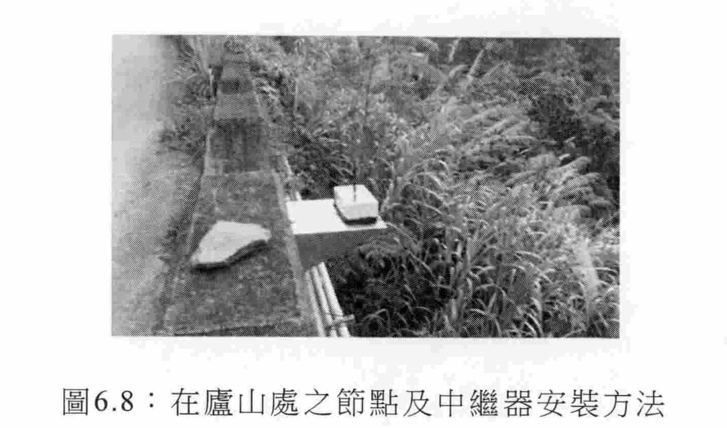
臺灣大約6月至10月往往會持續有季節性颱風。希望歸因於熱帶氣旋之大雨可能造成吾人可量測的地面變形。在2014颱風季節期間僅僅兩個熱帶氣旋衝擊臺灣;大約在2014年7月23日(204日)的稱為麥德姆之2類颱風及大約在2014年9月21日(264日)的稱為鳳凰之熱帶風暴。 Taiwan will continue to have seasonal typhoons from June to October. It is hoped that the heavy rain attributed to tropical cyclones may cause ground deformation that can be measured by us. During the 2014 typhoon season, only two tropical cyclones hit Taiwan; around July 23, 2014 (204), a type 2 typhoon called Medham and about September 21, 2014 (264 days) Tropical storm for the phoenix.

節點失效為顯著問題。節點274最終在2014年8月11日失效,節點275在2014年8月13日失效,且節點277在2014年12月21日失效。節點274及275正常進行直至其最終失 效。節點277在颱風麥德姆期間失效且此後兩天沒有傳回信號。節點277逐漸變得間歇,最終在2014年12月20日聽到最後信號而在2014年11月16日聽到倒數第二次信號。節點276幾乎完美地起作用且僅僅在熱帶氣旋鳳凰期間之三天確實無法傳輸任何信號。 Node failure is a significant problem. Node 274 eventually expired on August 11, 2014, node 275 expired on August 13, 2014, and node 277 expired on December 21, 2014. Nodes 274 and 275 proceed normally until they finally lose effect. Node 277 failed during Typhoon Modem and did not return a signal for the next two days. Node 277 gradually became intermittent, eventually hearing the last signal on December 20, 2014 and hearing the penultimate signal on November 16, 2014. Node 276 works almost perfectly and does not transmit any signals for only three days during the tropical cyclone.
完美且並非一天進行的基地台硬體及中繼器兩者被觀測,其中兩者中之任一者失效。 Both the base station hardware and the repeater, which are perfect and not one day, are observed, and either of them fails.
假定節點失效之原因係由進入電子電路並造成腐蝕及短路之水所引起。然而,因為吾人係以紐西蘭為基地,所以可並不容易地返回並檢查此等節點失效之原因。下圖展示在其失效之後某一時間的節點275。最初GPS天線為光亮的銀色而顯然在下圖中其失去光澤。天線係在RTV矽酮下方,RTV矽酮經設計以保護天線以對抗元件。在天線之右下角處的少量棕色亦大概被腐蝕。因此,似乎很可能此特定節點歸因於水破壞而失效。 It is assumed that the cause of node failure is caused by water entering the electronic circuit and causing corrosion and short circuit. However, because we are based in New Zealand, it is not easy to return and check the reasons for the failure of these nodes. The figure below shows node 275 at some time after its failure. The GPS antenna was originally bright silver and apparently lost its luster in the picture below. The antenna is below the RTV fluorene, and the RTV fluorene is designed to protect the antenna against the components. A small amount of brown at the lower right corner of the antenna is also likely to be corroded. Therefore, it seems likely that this particular node will fail due to water damage.
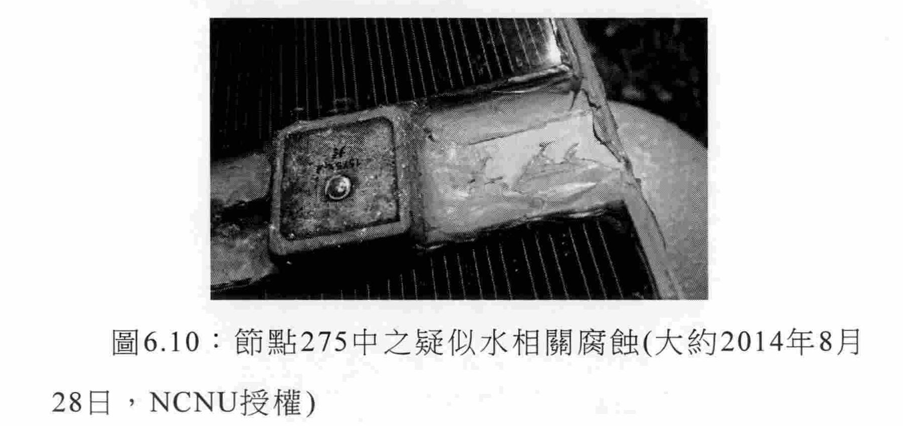
節點失效之另一疑似問題係植物過度生長。以下係在節點277間歇地失效時間期間的節點277之圖像。 Another suspected problem with node failure is plant overgrowth. The following is an image of node 277 during the intermittent failure time of node 277.

吾人自身先前設法建立不受水破壞影響之節點證明係困難的。在Paekakariki試驗台處在外面六個月之後,在開啟GPS接收器節點後就獲得以下圖像。如可看到,相當大量的水已進入殼體且亦設法在過去得到覆蓋PCB之保形塗層。實際上,由於PCB上之保形塗層,水不能排盡,從而使情形更糟。 It is difficult for us to try to establish a node that is not affected by water damage. After six months outside the Paekakariki test rig, the following image was obtained after turning on the GPS receiver node. As can be seen, a significant amount of water has entered the housing and has also managed to obtain a conformal coating covering the PCB in the past. In fact, due to the conformal coating on the PCB, the water cannot be drained, making the situation worse.
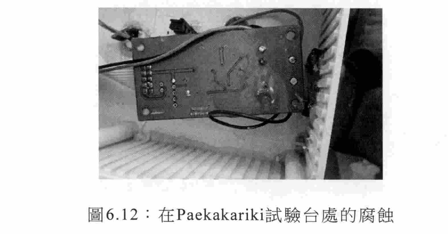
在廬山試驗台處在2014年年初,吾人發送最初GPS接收器節點以待於坡道上測試。截至吾人6月下旬到達,在開啟一個接收器節點後,就如可在下圖(圖6.13)中看到含有並 未排盡之熱水的殼體。吾人在7月放置在坡道上之新節點之殼體已經重新設計,且節點自身內部之PC板完全覆蓋在環氧樹脂中,惟程式設計接腳除外。GPS天線覆蓋在環氧樹脂中。吾人希望此將預防歸因於水破壞的節點失效。然而,吾人沒有足夠時間來預先嚴密進行測試。 At the Lushan Test Bench in early 2014, we sent the original GPS receiver node to be tested on the ramp. As we arrived in late June, after opening a receiver node, as seen in the figure below (Figure 6.13) The housing of the hot water that has not been drained. The shell of the new node that we placed on the ramp in July has been redesigned, and the PC board inside the node itself is completely covered in epoxy, except for the programming pins. The GPS antenna is covered in epoxy resin. We hope that this will prevent the failure of nodes attributed to water damage. However, we do not have enough time to test it in advance.
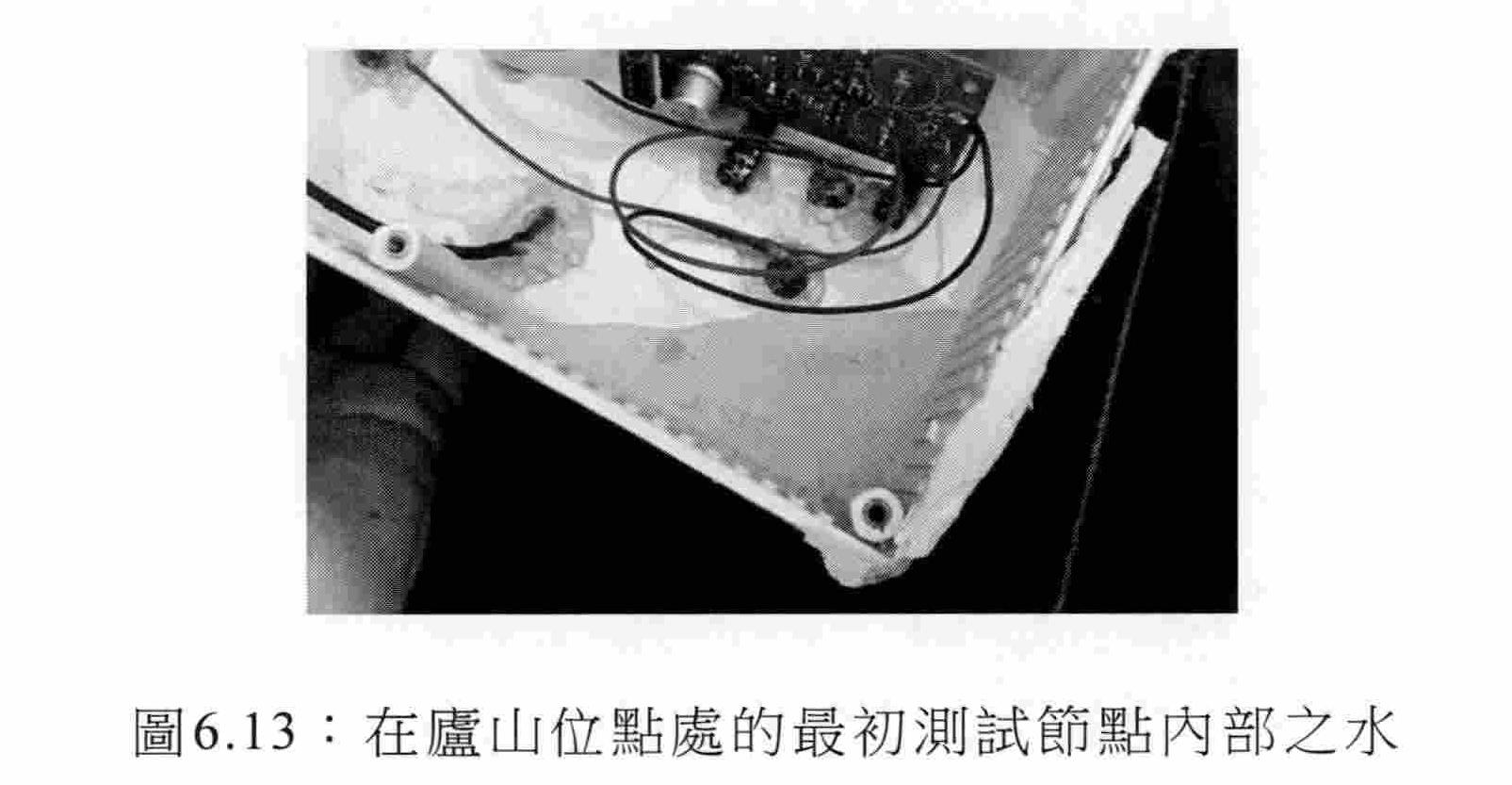
吾人希望使用節點274作為固定參考以便能夠量測與其他節點之相對位置。然而,因為節點274在安裝之後大約一月失效,所以上述希望在試驗台運行的大部分時間未實現。此使僅僅節點1及276在大部分時間內可用·節點1安裝在金屬I樑上,金屬I樑從前可能垂直但歸因於地面變形而有微向南傾斜坡度。此等節點皆在作用中滑動區帶上,意謂如沿著道路之壁與I樑頂部之間的長期關係的全部,吾人長期可希望量測。 We prefer to use node 274 as a fixed reference to be able to measure the relative position to other nodes. However, since node 274 failed approximately one month after installation, the above-mentioned hopes were not realized most of the time the test bed was in operation. This allows only nodes 1 and 276 to be available most of the time. Node 1 is mounted on a metal I beam that may have been vertically inclined from the front but may be slightly inclined to the south due to ground deformation. These nodes are all in the active sliding zone, meaning that as long as the long-term relationship between the wall of the road and the top of the I beam, we can hope to measure for a long time.
6.2.1相對於節點274之移動6.2.1 Movement relative to node 274
在以下圖中,吾人展示無線太陽能供電GPS接收器相對於節點274的NEU時間數列。此藉由採取相對於節點274的每一節點之間的最終解之差而進行。當採取解之間的差 時加性雜訊增加。然而,似乎在自相對於共同參考台的兩個不同節點獲得的解之間存在相當大的隨機相依性,此係大概因為類似日光條件造成觀測在兩個節點之間被相當類似地採取。因此,此方式獲得的解之精確度並不如吾人首先可能預測之精確度一般差。計算解之此方法具有以下優點:能夠使用在作用中滑動區帶上之永久供電參考台作為參考台使得最大化存在用於在給定太陽能供電GPS接收器上觀測之曆元之機率的優點,因此更多雙差可用於最終解。此與藉由使用兩個無線GPS接收器節點自身獲得雙差值且因此求解方位之方法進行對比;在此狀況下兩個GPS接收器節點必須同時獲得未必發生的雙差。另外,與建立兩個GPS接收器自身之間的雙差相比,非常容易減去最終解。 In the following figures, we show the NEU time series of wireless solar powered GPS receivers relative to node 274. This is done by taking the difference between the final solution between each node of node 274. When taking the difference between solutions Additive noise increased. However, it appears that there is considerable random dependence between solutions obtained from two different nodes relative to the common reference station, which is probably taken quite similarly between the two nodes because of similar daylight conditions. Therefore, the accuracy of the solution obtained in this way is not as good as the accuracy that we may first predict. This method of calculating the solution has the advantage that the ability to use the permanently powered reference station on the active sliding zone as a reference station maximizes the probability of having an epoch for observation on a given solar powered GPS receiver, Therefore more double differences can be used for the final solution. This is compared to the method of obtaining a double difference by using two wireless GPS receiver nodes themselves and thus solving the azimuth; in this case the two GPS receiver nodes must simultaneously obtain a double difference that does not necessarily occur. In addition, it is very easy to subtract the final solution compared to establishing a double difference between the two GPS receivers themselves.
對於下圖,吾人標繪運用實施如第2章中所描述之CFFS演算法的JAC-MM產生的NEU解。全部無線GPS接收器節點相對於節點274之時間數列被標繪,此係因為吾人被告知無274在非滑動區帶上。因為節點274在安裝之後不久失效,所以僅僅大約一月之解經標繪在諸圖中之每一者上。正好在第204日之前的黑色垂直線表示近似時間觀測將受颱風麥德姆影響。在277-274NEU時間數列圖中,兩個離群值被人工地移除,此係因為其顯著與解之剩餘部分不一致。 For the following figure, we plot the NEU solution generated by JAC-MM implementing the CFFS algorithm as described in Chapter 2. The time series of all wireless GPS receiver nodes relative to node 274 are plotted because we are told that no 274 is on the non-slip zone. Because node 274 fails shortly after installation, only about one month of interpretation is plotted on each of the figures. The black vertical line just before the 204th indicates that the approximate time observation will be affected by Typhoon Modham. In the 277-274 NEU time series chart, the two outliers are manually removed because they are significantly inconsistent with the rest of the solution.
使用獲得相對於節點274之相對解的此間接方式,忽略前14個解以允許恆星濾波穩定為3.3mm之平均2DRMS精 確度。 Using this indirect way of obtaining a relative solution relative to node 274, the first 14 solutions are ignored to allow the stellar filter to stabilize to an average 2DRMS fine of 3.3 mm. Exact.
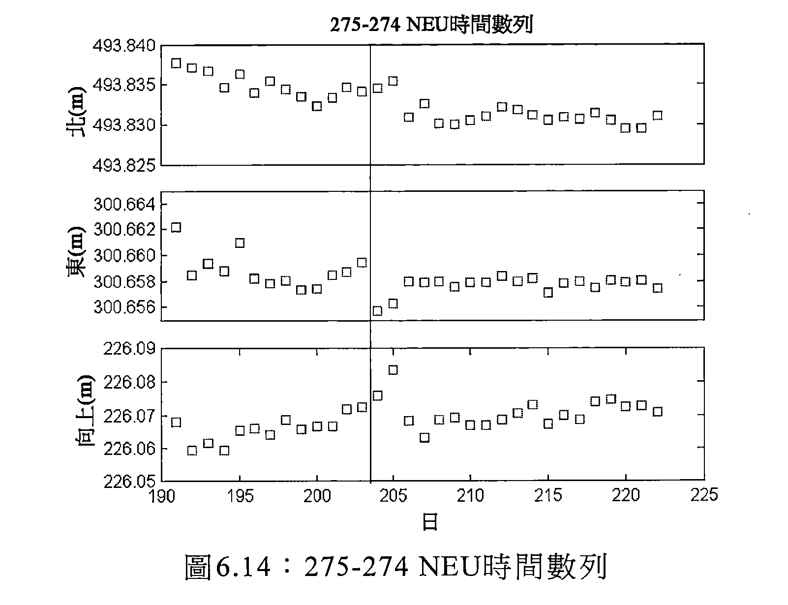
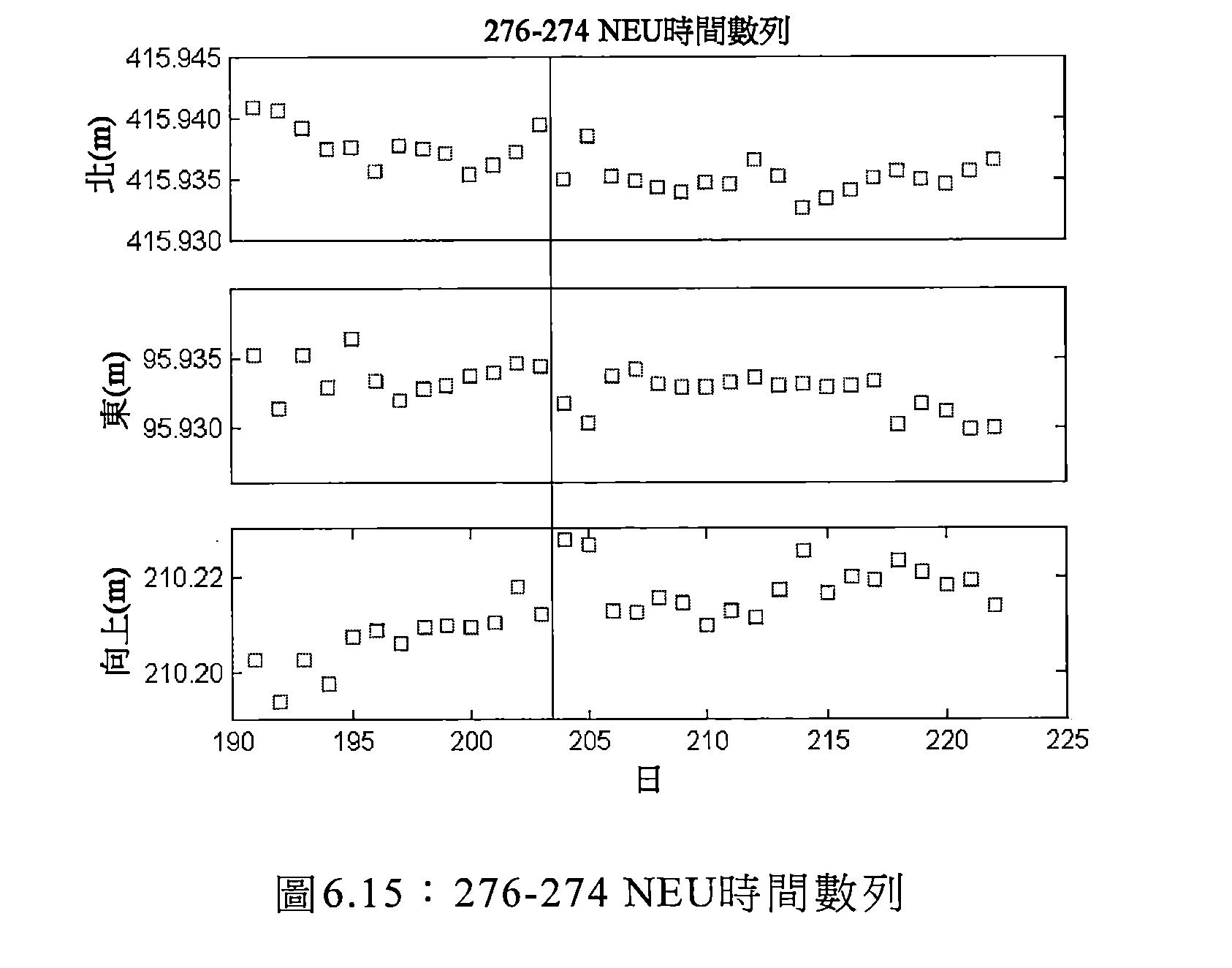

如可看到,不存在歸因於颱風麥德姆引起的顯著移動。在颱風之後約幾天的任何解偏差可歸因於雙差之缺少,此係因為陰天或土壤膨脹或一些其他暫時現象。全部節點具有在0.12mm/日至0.22mm/日之間的向南趨勢。節點277具有稍微向東分量而275及276具有極微小向西分量,全部節點具有在0.3mm/天至0.7mm/天之間的向上分量。不存在有力證據證實此在此短暫時間段內之極微小趨勢與任何地面變形有關,且完全可以想像其實際上為歸因於相對於太陽日之四分鐘恆星移位或節點隨著時間而沈降引起的在第3章中之模擬中預測的緩慢偏差變化。 As can be seen, there is no significant movement due to Typhoon Modham. Any deviation from the solution after a few days after the typhoon can be attributed to the lack of double difference, due to cloudy or soil swelling or some other temporary phenomenon. All nodes have a southward trend between 0.12 mm/day and 0.22 mm/day. Node 277 has a slightly eastward component and 275 and 276 have a very slight westward component, with all nodes having an upward component between 0.3 mm/day and 0.7 mm/day. There is no strong evidence that this extremely small trend during this short period of time is related to any ground deformation, and it is fully conceivable that it is actually due to a four-minute star shift relative to the sun's day or that the node settles over time. The resulting slow deviation change predicted in the simulation in Chapter 3.
6.2.2相對於節點1之277及2766.2.2 277 and 276 relative to node 1
在第222日之後從未再次聽到節點274。節點277愈來愈少聽到,而節點276截至書寫今天仍繼續。因此,此時吾人 比較相對於節點1之解且特定言之集中於相對於節點1之276,此係因為此對大部分始終在作用中。 Node 274 is never heard again after day 222. Node 277 is less and less heard, and node 276 continues as of today. Therefore, at this time, I am Comparing the solution with respect to node 1 and specifically focusing on 276 relative to node 1, this is because most of this pair is always active.
下圖展示節點277相對於節點1(277-1)之NEU時間數列解。正好在第264日之前的第二中心黑色垂直線表示熱帶風暴鳳凰可能影響解之時間。 The figure below shows the NEU time series solution of node 277 relative to node 1 (277-1). The black vertical line in the second center just before the 264th day indicates that the Tropical Storm Phoenix may affect the time of the solution.
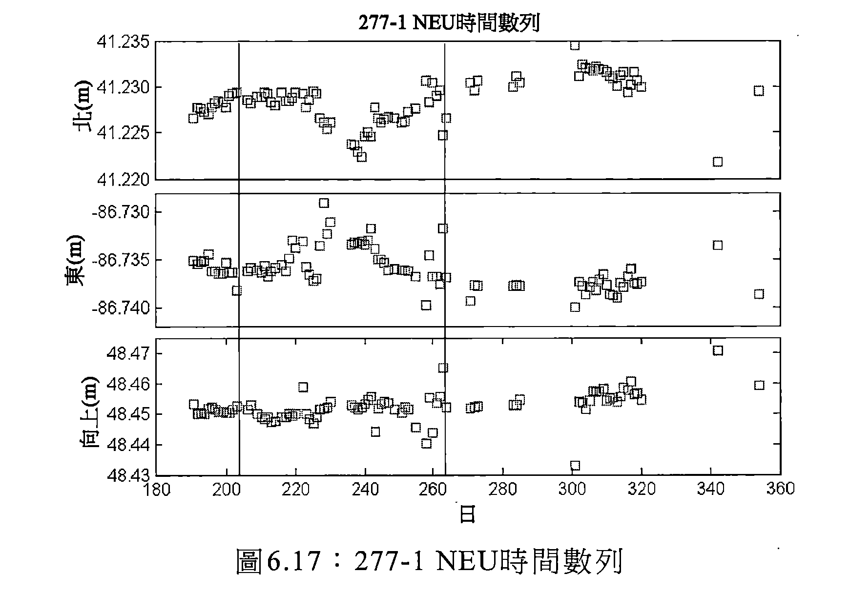
如可看到,顯著異常以約日期230為中心發生並延伸至少10日至日期之任一側。在北方向上存在約5mm之下降而同時在東方向上存在大約相同量值之上升;此並不為吾人知曉。如可看到,在熱帶風暴鳳凰衝擊之日附近並不存在顯著改變。如同到目前為止對於廬山展示的全部解,在向上方向上存在緩慢大約線性增加;在此狀況下約0.03mm/日至0.05mm/日。 As can be seen, significant abnormalities occur around the date 230 and extend at least 10 days to either side of the date. There is a drop of about 5 mm in the north and an increase in the same magnitude in the east; this is not known to us. As can be seen, there is no significant change around the day of the Tropical Storm Phoenix impact. As with all solutions so far for the Lushan show, there is a slow linear increase in the upward direction; in this case about 0.03 mm/day to 0.05 mm/day.
下圖展示使用JAC-MM獲得的276-1之東北向上時間數列解。 The figure below shows the northeast up time series solution of 276-1 obtained using JAC-MM.

在大約第340日至第360日之間存在雜訊之異常增加,此係在12月期間。吾人認為此雜訊係由於道路施工,因為在此時間期間道路瀝青中之一些被替換,經過感測器之重型機械可能使其振動。然而,遠離道路施工之月,解一般係非常精確且在其被獲得的七個月內緩慢改變。因為此係吾人之持續最大時間段的測試,所以吾人視為七個月足夠接近於12個月,期間吾人可至少獲得系統(諸如吾人之系統)將在典型設定中具有的預期準確度之想法。若節點276並不移動及/或其周圍環境並不改變,則忽略前14日以允許恆星濾波將內部解準確度穩定為9.12mm 2DRMS;當然,此僅僅在不存在移動或周圍環境不改變之情況下有效。此 亦可大約視為內部準確度之最差狀況。另一方面,若解之緩慢改變由節點自身之實體移動引起,則使用10次多項式擬合以移除解之緩慢改變,獲得大約3.6mm之2DRMS內部準確度;此可被視為解準確度之最佳狀況且亦被視為解精確度。 There was an abnormal increase in noise between about 340th and 360th, which was during the December period. I think this noise is due to road construction, because some of the road asphalt is replaced during this time, and heavy machinery passing through the sensor may vibrate it. However, away from the month of road construction, the solution is generally very accurate and slowly changes within seven months of its acquisition. Because this is our continuous maximum time period test, we consider it to be close enough to 12 months in seven months, during which we can at least get the idea that the system (such as our system) will have the expected accuracy in the typical setting. . If node 276 does not move and/or its surrounding environment does not change, the first 14 days are ignored to allow stellar filtering to stabilize the internal solution accuracy to 9.12 mm 2DRMS; of course, this is only in the absence of movement or the surrounding environment does not change. It is effective in the case. this It can also be considered as the worst case of internal accuracy. On the other hand, if the slow change of the solution is caused by the physical movement of the node itself, a 10 degree polynomial fit is used to remove the slow change of the solution, achieving a 2DRMS internal accuracy of approximately 3.6 mm; this can be considered as the solution accuracy The best condition is also considered to be the accuracy of the solution.
首先,吾人應注意,向上方向在非線性方面不同於節點277,東解平滑地波動而北解相當平坦直至第310日,在第310日中其快速下降而同時向上方向快速增加。吾人注意到最顯著的事係,正好在熱帶風暴鳳凰之前獲得的向上解顯著高於正好在該風暴之後獲得的向上解。同時在北解中亦存在相當顯著快速改變。另外,解之改變率在風暴之前及之後突然改變。若吾人在第242日與第287日(包含端點)之間獲得主要主分量方向向量,則可較好看到此等快速改變,且標繪此等解,如在下圖中可看到。 First, we should note that the upward direction differs from the node 277 in terms of nonlinearity, the east solution fluctuates smoothly and the north solution is fairly flat until the 310th day, during which it rapidly drops while the upward direction increases rapidly. I noticed the most striking fact that the upward solution obtained just before the Tropical Storm Phoenix was significantly higher than the upward solution obtained just after the storm. At the same time, there is also a fairly significant rapid change in the North Solution. In addition, the rate of change of the solution suddenly changed before and after the storm. If we obtain the main principal component direction vector between 242th and 287th (including the endpoint), we can see these fast changes better, and plot these solutions, as can be seen in the figure below.
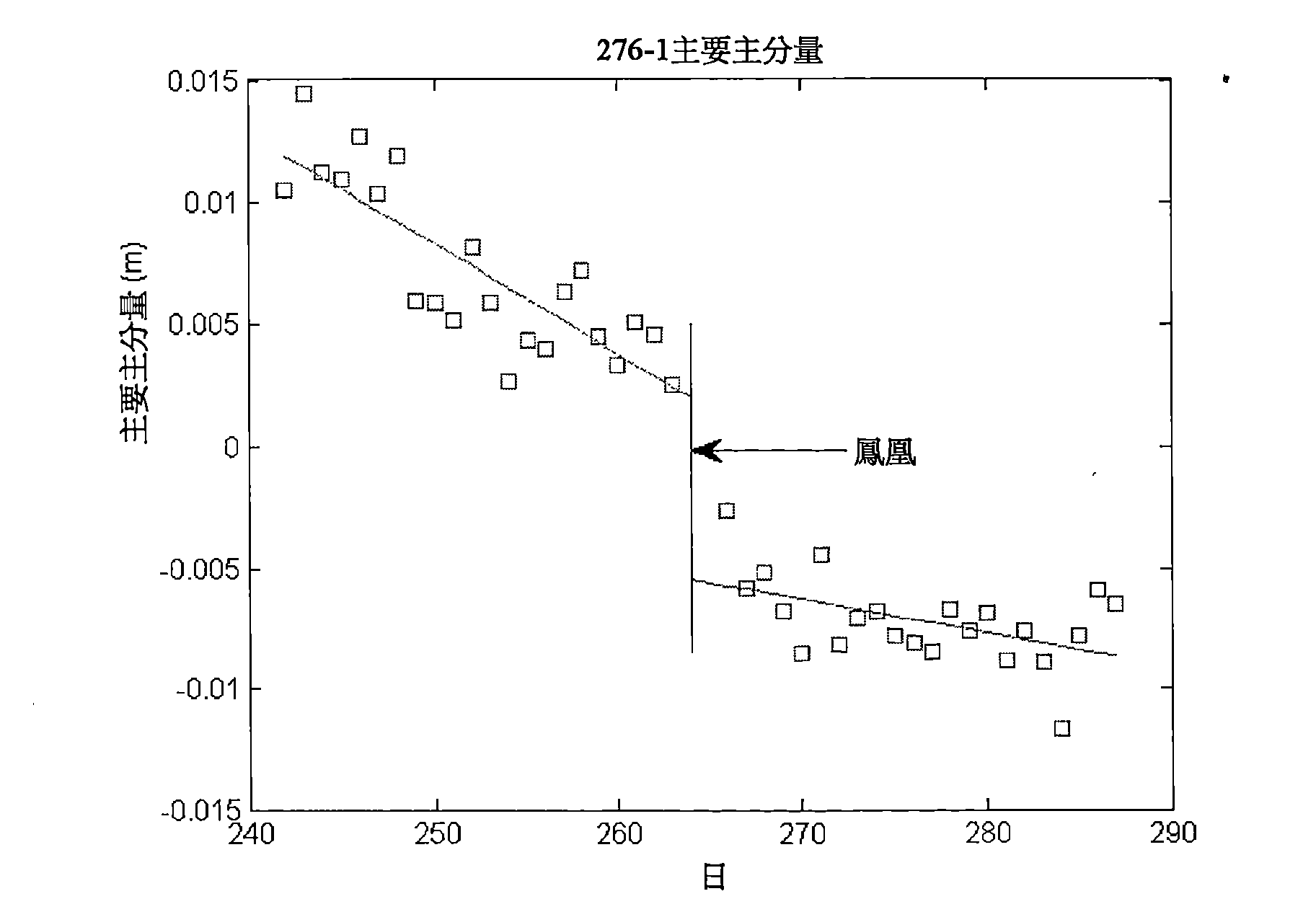
此圖大約展示在氣旋之前的20日及在氣旋之後的20日。綠線及紫線分別為針對在氣旋之前及之後的時間之線性擬合。解在氣旋之前及在氣旋之後以不同速率改變。另外,兩個線性擬合在氣旋時失配7.45mm。解看起來亦繞其線性擬合大體上正態分佈。吾人接著藉由自此等解中移除線性趨勢而估計此位移之準確度以獲得具有點線標準差之下圖。 This figure shows approximately 20 days before the cyclone and 20 days after the cyclone. The green and purple lines are respectively a linear fit for the time before and after the cyclone. The solution changes at different rates before and after the cyclone. In addition, the two linear fits mismatched 7.45 mm at cyclonic. The solution also appears to have a substantially normal distribution around its linear fit. We then estimate the accuracy of this displacement by removing the linear trend from this solution to obtain a plot with a dotted line standard deviation.
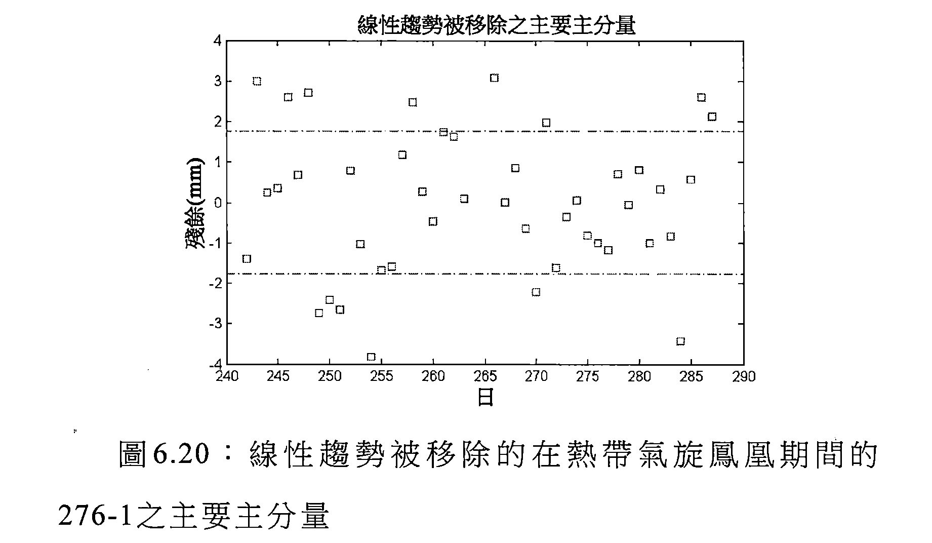
如可看到,其看起來為具有1.758mm之標準差的相當正態分佈。因此,吾人應獲得所量測之移動關於吾人之估計為
吾人並不將解導數之不連續性完全理解為其不在吾人之模擬中出現。圖6.18中之一個顯著不連續性係在約第315日在向上方向中,其亦伴隨著北方向上之緩慢下降。此恰巧符合3.6量級及4.9km深度之小較淺地震,非常接近但可恰好重合。 We do not fully understand the discontinuity of the derivation number as it does not appear in our simulations. One of the significant discontinuities in Figure 6.18 is in the upward direction about 315 days, which is also accompanied by a slow decline in the north. This coincides with a small shallow earthquake of magnitude 3.6 and a depth of 4.9 km, which is very close but can coincide.
6.2.3與逆向反射器觀測之比較6.2.3 Comparison with retroreflector observations
下圖展示在位點處之逆向反射器之位置。綠色逆向反射器為在作用中滑移區帶外部並用於滑移區帶中之反射器的相對定位的逆向反射器。 The figure below shows the position of the retroreflector at the site. The green retroreflector is a retroreflector that is external to the active slip zone and is used for relative positioning of the reflectors in the slip zone.
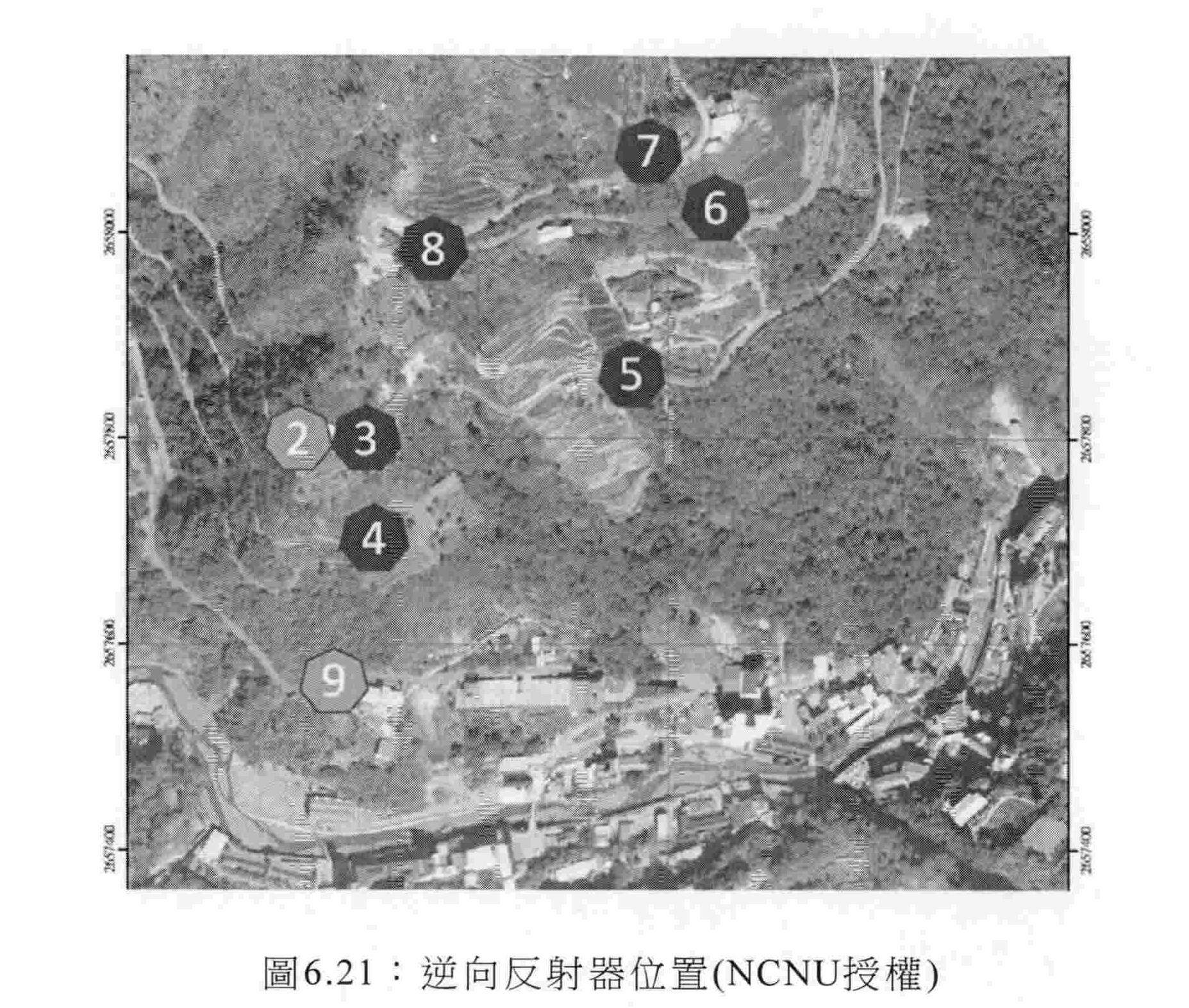
如可看到,不存在裝配於吾人之基地台之GPS接收器節點1的位點處的逆向反射器。逆向反射器8緊鄰於吾人之節點276定位,而逆向反射器9緊鄰於吾人之節點274。由NCNU使用之總台為Trimble S8;根據NCNU,其自Trimble接收之報告說距離準確度為2mm±1ppm且角度準確度為0.5",但吾人並未被通知此等準確度類型係什麼。自Trimble S8資料表[56],存在對於不同情形給出之許多不同準確度;其中使用逆向反射器,全部準確度係大約相同數量級且經給定為用於距離之RMSE及用於角度之標準差。對於在「DR HP」下之效能,距離準確度1mm+1ppm RMSE及0.5"標準差之角度準確度。因此,吾人假定距離準確度2 mm+1ppm RMSE及0.5"標準差之角度準確度,其大約匹配於如資料表中給出之「DR HP」效能,且數目極類似於由NCNU給予吾人之數目。總台置放於位點正南大約一公里;角度準確度及距離準確度以及定向可在下圖中看到。 As can be seen, there is no retroreflector at the location of the GPS receiver node 1 of the base station of ours. The retroreflector 8 is positioned next to the node 276 of ours, and the retroreflector 9 is adjacent to the node 274 of our person. The total station used by the NCNU is the Trimble S8; according to the NCNU, the report received from Trimble has a distance accuracy of 2 mm ±1 ppm and an angular accuracy of 0.5", but we have not been notified of what these accuracy types are. From the Trimble S8 data sheet [56], there are many different accuracies given for different situations; where retroreflectors are used, all accuracy is about the same order of magnitude and is given for the RMSE for distance and for angles Standard deviation. For performance under "DR HP", distance accuracy is 1 mm +1 ppm RMSE and angular accuracy of 0.5" standard deviation. Therefore, we assume distance accuracy of 2 mm +1 ppm RMSE and 0.5" standard deviation The angular accuracy is approximately matched to the "DR HP" performance as given in the data sheet, and the number is very similar to the number given to us by the NCNU. The total stage is placed approximately one kilometer south of the site; angular accuracy and distance accuracy and orientation can be seen in the figure below.
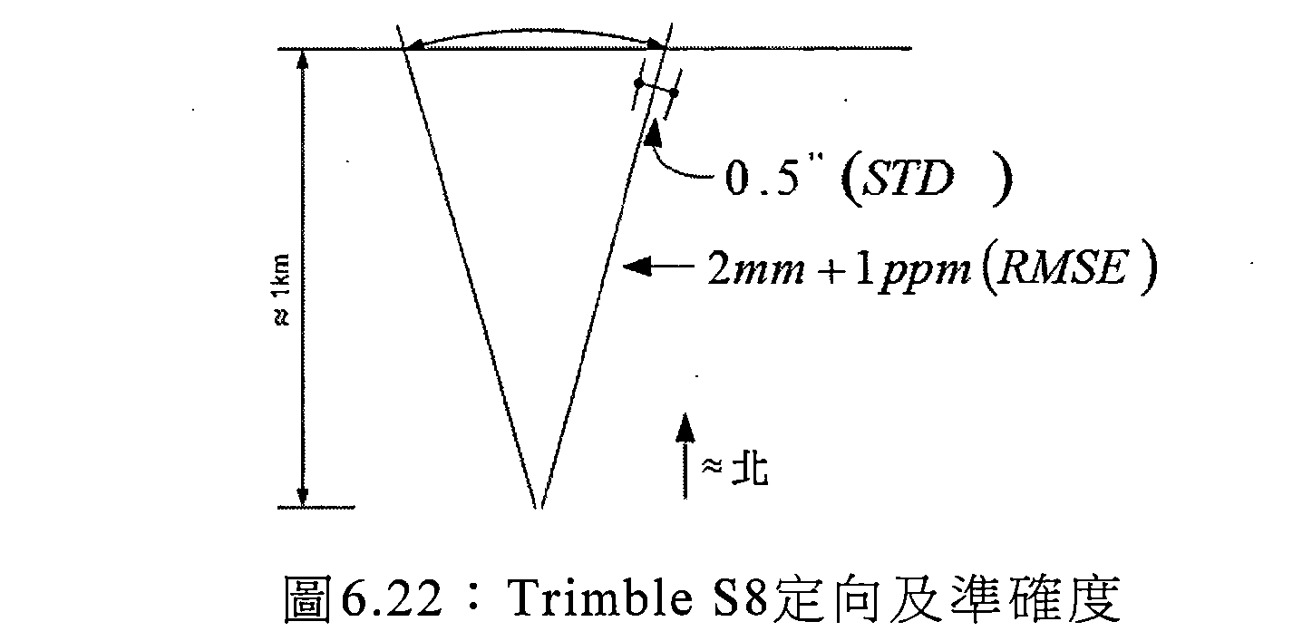
為了獲得應自總台預期什麼3D準確度之想法,導出極近似估計。對於東及向上準確度,吾人使用假定關於北軸之旋轉對稱性的小角度近似,而北準確度之假定僅為共台之距離準確度。進行此意謂東及向上方向中之標準差為約

以下三個圖展示自2013年11月8日以來至如顏色所指示之日期的逆向反射器相對於逆向反射器2及9的總位移。舉例而言,在2014年7月2日與2014年8月28日之間,逆向反射器6在第57日向南移動10mm。 The following three figures show the total displacement of the retroreflector relative to retroreflectors 2 and 9 from November 8, 2013 to the date indicated by the color. For example, between July 2, 2014 and August 28, 2014, the retroreflector 6 moved 10 mm south on the 57th day.
吾人關注逆向反射器8,此係因為此對應於吾人之節點276,且吾人關注逆向反射器3及4,此係因為此等接近於吾人之節點1且因此吾人將預期到地面之移動更可能類似於 其他逆向反射器。 I am concerned about retroreflector 8, which is because this corresponds to node 276 of ours, and we are concerned with retroreflectors 3 and 4, because this is close to our node 1 and therefore we are expected to move to the ground more likely Similar to Other retroreflectors.


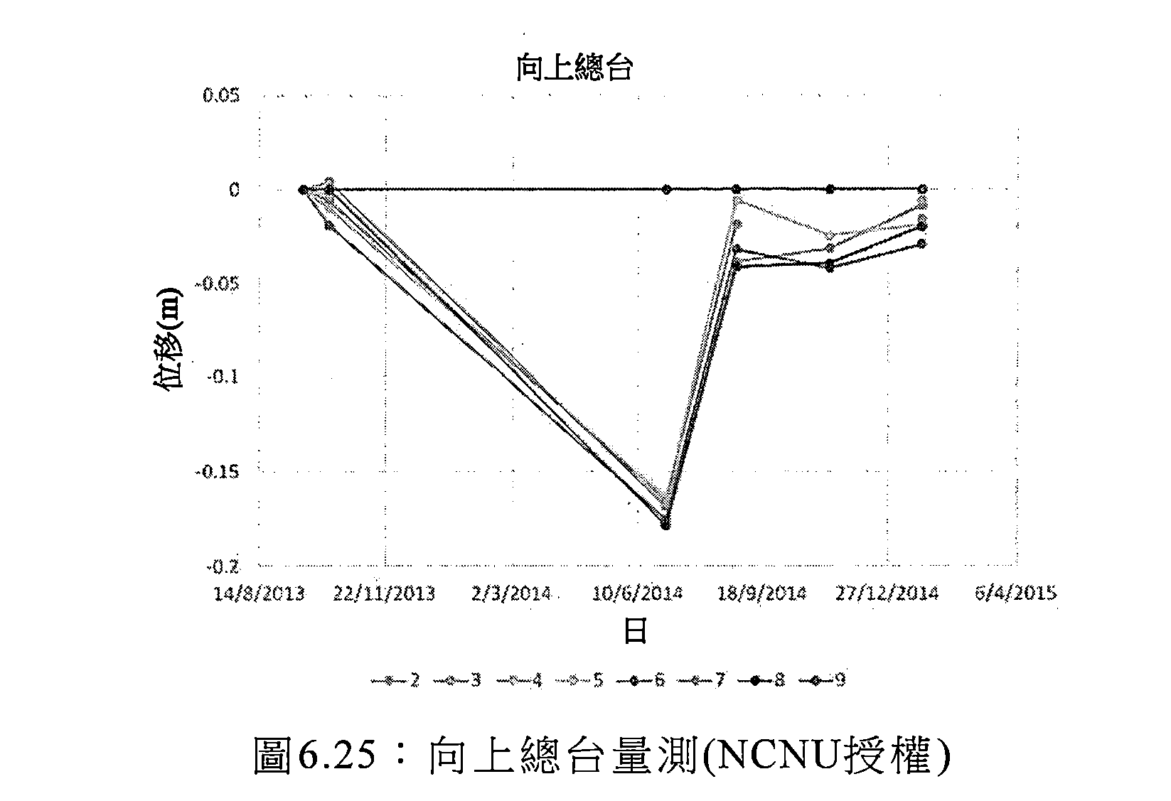
如可看到,存在使用總台獲得之解的一些相當大的改變;第三向上解及第四東解顯著遠離吾人將預期的解。每當總台用以獲得量測時亦出現解之相當大的相關性,如可看到,當一個解向南移動時全部其他解往往會同時移動。量測之稀疏性係有問題的,此係因為此使得難以知曉量測可靠性如何。在全部解之中,北解似乎為最一致且展示如所預期之緩慢向南的一般趨勢。東解及向上解兩者甚至在移除在7月及8月進行之量測之後似乎仍不能說大量。顯然存在引入至此等解中之顯著大於吾人估計之誤差的其他誤差。歸因於此等其他誤差,不知曉坡道之實際移動如何與總台量測相關。雖然不令人滿意,但吾人實際上不能比較GPS解與總台解。 As can be seen, there are some considerable changes in the solution obtained using the main station; the third upward solution and the fourth east solution are significantly far from the solution that we would expect. There is also a considerable correlation of the solution whenever the total station is used to obtain the measurements. As can be seen, all of the other solutions tend to move simultaneously as one solution moves south. The sparsity of the measurement is problematic because it makes it difficult to know the reliability of the measurement. Among all the solutions, the North Solution seems to be the most consistent and shows the general trend of slow southward as expected. Both East and Up Solutions seem to be unable to say a lot after removing the measurements taken in July and August. Obviously there are other errors introduced into these solutions that are significantly larger than the error estimated by us. Due to these other errors, it is not known how the actual movement of the ramp is related to the total station measurement. Although it is not satisfactory, we can't actually compare the GPS solution with the total solution.
總台量測係時間稀疏且可變的,從而使結論困難。用於瞬時移動(亦即,不緩慢且連續之移動)之GPS解如吾人對於歸因於熱帶風暴鳳凰之解改變所說顯然極精確。對比 而言,難以自GPS解對GPS接收器在六個月內之長期移動作出結論。此係因為自多路徑及恆星濾波,吾人預測歸因於多路徑偏差之解分量,其經預測為在年內改變,從而使得難以區分真實移動與僅緩慢改變的解偏差。另外,在節點274失效之前在7月可僅僅比較GPS移動。然而,在此月中,GPS接收器全部展示相對於被給定為靜止的節點274之微小南向趨勢,此匹配自總台獲得的北解之變化的一般趨勢與吾人將預期之趨勢。 The total station measurement time is sparse and variable, making the conclusion difficult. The GPS solution for instantaneous movement (i.e., non-slow and continuous movement) is as apparently accurate as the solution due to the tropical storm phoenix. Compared In terms of difficulty, it is difficult to conclude from the GPS solution to the long-term movement of the GPS receiver within six months. This is because, since multipath and stellar filtering, we predict the solution component due to multipath bias, which is predicted to change during the year, making it difficult to distinguish between true and only slowly changing solution deviations. In addition, only GPS movements can be compared in July before node 274 fails. However, during the month, the GPS receivers all show a slight southward trend relative to the node 274 that is given a standstill, which matches the general trend of the change in the North Solution obtained from the total station and the trend that we would expect.
110‧‧‧無線感測器網路(WSN) 110‧‧‧Wireless Sensor Network (WSN)
116A、116B、116C‧‧‧節點 116A, 116B, 116C‧‧‧ nodes
400‧‧‧系統 400‧‧‧ system
402‧‧‧代碼模組 402‧‧‧ Code Module
404‧‧‧浮動模組 404‧‧‧ Floating Module
406‧‧‧固定模組 406‧‧‧Fixed modules
408‧‧‧恆星模組 408‧‧‧Star Module
Claims (30)
Applications Claiming Priority (2)
| Application Number | Priority Date | Filing Date | Title |
|---|---|---|---|
| ??719310 | 2016-04-22 | ||
| NZ71931016 | 2016-04-22 |
Publications (1)
| Publication Number | Publication Date |
|---|---|
| TW201802492A true TW201802492A (en) | 2018-01-16 |
Family
ID=60116681
Family Applications (1)
| Application Number | Title | Priority Date | Filing Date |
|---|---|---|---|
| TW106113658A TW201802492A (en) | 2016-04-22 | 2017-04-24 | Method and system for monitoring land deformation |
Country Status (5)
| Country | Link |
|---|---|
| US (1) | US11163070B2 (en) |
| AU (1) | AU2017252079A1 (en) |
| NZ (1) | NZ747152A (en) |
| TW (1) | TW201802492A (en) |
| WO (1) | WO2017183005A1 (en) |
Cited By (4)
| Publication number | Priority date | Publication date | Assignee | Title |
|---|---|---|---|---|
| CN116432694A (en) * | 2021-12-30 | 2023-07-14 | 浙江舜宇智能光学技术有限公司 | Compression method and device based on neural network model for eliminating TOF multipath |
| TWI852221B (en) * | 2022-12-15 | 2024-08-11 | 立積電子股份有限公司 | Object sensing method and radar apparatus |
| CN118626952A (en) * | 2024-05-29 | 2024-09-10 | 无锡承方科技有限公司 | Automatic recognition system of seismic wave signals based on machine learning |
| CN119936920A (en) * | 2024-12-30 | 2025-05-06 | 上海移为通信技术股份有限公司 | NTN signal transmission direction adjustment method, device, storage medium and product |
Families Citing this family (10)
| Publication number | Priority date | Publication date | Assignee | Title |
|---|---|---|---|---|
| CN108537360A (en) * | 2018-03-01 | 2018-09-14 | 长安大学 | One kind taking polyfactorial adaptable Kalman filter slide prediction method into account |
| US11172423B2 (en) | 2018-12-31 | 2021-11-09 | Itron, Inc. | Solar-powered access point for load balancing network traffic across backhaul networks |
| US11296539B2 (en) | 2018-12-31 | 2022-04-05 | Itron, Inc. | Solar hybrid battery for powering network devices over extended time intervals |
| US11184831B2 (en) | 2018-12-31 | 2021-11-23 | Itron, Inc. | Solar-powered relay for coupling remotely-located leaf nodes to a wireless network |
| CN110068849A (en) * | 2019-05-06 | 2019-07-30 | 国网山东省电力公司东营供电公司 | Transmission line of electricity multidimensional deformation method of real-time and system based on Differential positioning |
| CN112073996B (en) * | 2019-06-10 | 2022-08-09 | 华为技术有限公司 | Operator information updating method and device |
| US11914051B2 (en) | 2019-11-20 | 2024-02-27 | Tupaia | System and method for determining accurate positions of stationary global navigation satellite system sensors |
| CN111641490B (en) * | 2020-05-20 | 2021-07-09 | 中国人民解放军国防科技大学 | A high-precision phase calibration and time reference determination method for sampling clock |
| CN112180830B (en) * | 2020-10-13 | 2021-05-25 | 广东省地质建设工程勘察院 | Geological disaster early warning monitoring devices |
| CN119124053B (en) * | 2024-08-23 | 2026-01-30 | 武汉大学 | A geological disaster deformation monitoring method based on the BeiDou satellite navigation system |
Family Cites Families (17)
| Publication number | Priority date | Publication date | Assignee | Title |
|---|---|---|---|---|
| US5148179A (en) * | 1991-06-27 | 1992-09-15 | Trimble Navigation | Differential position determination using satellites |
| JP2816948B2 (en) * | 1995-04-20 | 1998-10-27 | 株式会社レイディック | Landslide surface movement measurement device |
| US5991691A (en) * | 1997-02-20 | 1999-11-23 | Raytheon Aircraft Corporation | System and method for determining high accuracy relative position solutions between two moving platforms |
| US6570530B2 (en) * | 2001-03-05 | 2003-05-27 | Qualcomm Incorporated | Method and apparatus providing improved position estimate based on an initial coarse position estimate |
| JP4116792B2 (en) | 2001-12-19 | 2008-07-09 | 古野電気株式会社 | Carrier phase relative positioning device |
| ITTO20050065A1 (en) * | 2005-02-04 | 2006-08-05 | Sepa Sistemi Elettronici | SYSTEM AND METHOD OF MONITORING AND SURVEILLANCE OF LAND MOVEMENTS, LARGE INFRASTRUCTURE AND CIVIL CONSTRUCTION WORKS IN GENERAL, BASED ON SIGNALS SENT BY THE GPS SATELLITE NAVIGATION SYSTEM |
| US7702460B2 (en) * | 2006-06-17 | 2010-04-20 | Northrop Grumman Guidance And Electronics Company, Inc. | Estimate of relative position between navigation units |
| WO2009000314A1 (en) * | 2007-06-22 | 2008-12-31 | Trimble Terrasat Gmbh | Position tracking device and method |
| US8174437B2 (en) * | 2009-07-29 | 2012-05-08 | Hemisphere Gps Llc | System and method for augmenting DGNSS with internally-generated differential correction |
| US7961145B1 (en) * | 2010-05-07 | 2011-06-14 | Sri International | Method and apparatus for estimating relative position in a global navigation satellite system |
| US9846241B2 (en) * | 2010-07-30 | 2017-12-19 | Deere & Company | Navigation system and method using RTK with data received from a mobile base station |
| JP5884960B2 (en) * | 2011-03-18 | 2016-03-15 | セイコーエプソン株式会社 | Position detection system |
| US9529093B2 (en) * | 2012-10-12 | 2016-12-27 | Google Inc. | Systems and methods for estimating attitude using double differenced GPS carrier phase measurements |
| WO2016163910A1 (en) * | 2015-04-09 | 2016-10-13 | Limited Liability Company "Topcon Positioning Systems" | Reducing time and increasing reliability of ambiguity resolution in gnss |
| WO2019083523A1 (en) * | 2017-10-23 | 2019-05-02 | Deere & Company | Rtk vector phase locked loop architecture |
| US10775513B1 (en) * | 2018-04-18 | 2020-09-15 | Topcon Positioning Systems, Inc. | High performance positioning system based on GNSS receiver with multiple front ends |
| US11402483B2 (en) * | 2019-01-07 | 2022-08-02 | Niiva OpCo, LLC | Systems and methods to detect motion on sloped surfaces |
-
2017
- 2017-04-24 TW TW106113658A patent/TW201802492A/en unknown
- 2017-04-24 US US16/095,401 patent/US11163070B2/en not_active Expired - Fee Related
- 2017-04-24 AU AU2017252079A patent/AU2017252079A1/en not_active Abandoned
- 2017-04-24 WO PCT/IB2017/052328 patent/WO2017183005A1/en not_active Ceased
- 2017-04-24 NZ NZ747152A patent/NZ747152A/en not_active IP Right Cessation
Cited By (5)
| Publication number | Priority date | Publication date | Assignee | Title |
|---|---|---|---|---|
| CN116432694A (en) * | 2021-12-30 | 2023-07-14 | 浙江舜宇智能光学技术有限公司 | Compression method and device based on neural network model for eliminating TOF multipath |
| TWI852221B (en) * | 2022-12-15 | 2024-08-11 | 立積電子股份有限公司 | Object sensing method and radar apparatus |
| US12546876B2 (en) | 2022-12-15 | 2026-02-10 | Richwave Technology Corp. | Object sensing method and radar apparatus |
| CN118626952A (en) * | 2024-05-29 | 2024-09-10 | 无锡承方科技有限公司 | Automatic recognition system of seismic wave signals based on machine learning |
| CN119936920A (en) * | 2024-12-30 | 2025-05-06 | 上海移为通信技术股份有限公司 | NTN signal transmission direction adjustment method, device, storage medium and product |
Also Published As
| Publication number | Publication date |
|---|---|
| US11163070B2 (en) | 2021-11-02 |
| NZ747152A (en) | 2022-01-28 |
| AU2017252079A1 (en) | 2018-11-22 |
| WO2017183005A1 (en) | 2017-10-26 |
| US20190137631A1 (en) | 2019-05-09 |
| AU2017252079A2 (en) | 2019-03-14 |
Similar Documents
| Publication | Publication Date | Title |
|---|---|---|
| TW201802492A (en) | Method and system for monitoring land deformation | |
| CN110275186B (en) | LEO satellite enhanced GNSS ionosphere normalization and fusion modeling method | |
| CN103376454B (en) | Advanced GLONASS using precise satellite Information locating(GNSS) | |
| CN111983654B (en) | Method for constructing ionosphere phase scintillation factor in arctic region based on GNSS | |
| Lu et al. | Multipath mitigation in GNSS precise point positioning based on trend-surface analysis and multipath hemispherical map | |
| RU2479855C2 (en) | Distance dependant error mitigation in real-time kinematic positioning | |
| JP2022530983A (en) | Systems and methods for high integrity satellite positioning | |
| US20150369924A1 (en) | Method and system for high-accuracy differential tracking of global positioning system (gps) receivers | |
| CN103748480A (en) | Coding in Wide Area Positioning System (WAPS) | |
| CN104483691B (en) | A kind of GNSS combines accurate one-point positioning method | |
| CN107462901A (en) | For the method and system from transmitter network launches positioning signal | |
| CN113985455A (en) | High-precision ionosphere modeling method fusing multi-source ionosphere observation data | |
| CN103336290A (en) | A method and a system for measuring baselines between adjacent formation satellites | |
| Jin et al. | Atmospheric sounding from fengyun‐3c gps radio occultation observations: First results and validation | |
| WO2006082520A2 (en) | A system and method for monitoring and surveying movements of the terrain, large infrastructures and civil building works in general, based upon the signals transmitted by the gps navigation satellite system | |
| CN117111112B (en) | GNSS and LNSS data fusion processing method and system | |
| Wu | Performance of regional atmospheric error models for NRTK in GPSnet and the implementation of a NRTK system | |
| Sun et al. | Real-time precise point positioning performance in Hong Kong during May 2024 space weather events | |
| Wang et al. | Long-term time-varying characteristics of UPD products generated by a global and regional network and their interoperable application in PPP | |
| Mushini et al. | Use of varying shell heights derived from ionosonde data in calculating vertical total electron content (TEC) using GPS–New method | |
| Luo et al. | Improved GNSS-IR height measurement method based on locally weighted regression | |
| Das et al. | Simplistic approach for water vapour sensing using a standalone global positioning system receiver | |
| Olds | Small batteryless wireless solar powered GPS receivers for subcentimeter land deformation monitoring | |
| Chen | Real-time precise point positioning, timing and atmospheric sensing | |
| Xu et al. | Determining of Geopotential Difference with Multi-GNSS Undifferenced Time-Frequency Signals |