WO2012111118A1 - 高速最適化装置、およびプログラム - Google Patents
高速最適化装置、およびプログラム Download PDFInfo
- Publication number
- WO2012111118A1 WO2012111118A1 PCT/JP2011/053325 JP2011053325W WO2012111118A1 WO 2012111118 A1 WO2012111118 A1 WO 2012111118A1 JP 2011053325 W JP2011053325 W JP 2011053325W WO 2012111118 A1 WO2012111118 A1 WO 2012111118A1
- Authority
- WO
- WIPO (PCT)
- Prior art keywords
- analysis
- experimental
- experimental point
- point
- model
- Prior art date
- Legal status (The legal status is an assumption and is not a legal conclusion. Google has not performed a legal analysis and makes no representation as to the accuracy of the status listed.)
- Ceased
Links
Images





Classifications
-
- G—PHYSICS
- G06—COMPUTING OR CALCULATING; COUNTING
- G06F—ELECTRIC DIGITAL DATA PROCESSING
- G06F30/00—Computer-aided design [CAD]
- G06F30/20—Design optimisation, verification or simulation
-
- G—PHYSICS
- G06—COMPUTING OR CALCULATING; COUNTING
- G06F—ELECTRIC DIGITAL DATA PROCESSING
- G06F2111/00—Details relating to CAD techniques
- G06F2111/04—Constraint-based CAD
-
- G—PHYSICS
- G06—COMPUTING OR CALCULATING; COUNTING
- G06F—ELECTRIC DIGITAL DATA PROCESSING
- G06F2111/00—Details relating to CAD techniques
- G06F2111/10—Numerical modelling
Definitions
- Patent Literature 1 a new design variable to be newly analyzed and an analysis have already been performed in a design support device that obtains an optimum shape of an air supply port that satisfies a target evaluation index by numerical fluid calculation. Determine whether past design variables are similar, determine whether the analysis result of the evaluation index is accompanied by flow separation, and the new design variables are similar to past design variables If it is determined that the evaluation index is analyzed, the analysis result of the evaluation index for the new design variable is assigned the analysis result of the evaluation index for the past design variable that is similar to the new design variable and does not involve separation.
- a technique for obtaining an optimum shape of an air supply port at high speed is disclosed.
- Patent Document 1 The invention described in Patent Document 1 is effective for shortening the analysis time.
- an analysis model that has already been analyzed and an analysis result database in which the analysis results are sufficiently stored are required. Therefore, an object of the present invention is to provide a method for efficiently reducing the analysis time even when there is no analysis result database.
- the present invention is configured as follows.
- the high-speed optimization device of the present invention is a high-speed optimization device that performs numerical analysis related to a predetermined design variable space of a shape template model of three-dimensional CAD (Computer Aided Design) data to obtain an optimal solution, Based on an analysis order determining unit that determines an analysis order of a plurality of experimental points in a predetermined design variable space and outputs an analysis order-determined experimental point group, and the design variable information related to the shape template model and the first experimental point An analysis model creation unit that creates a first analysis model, an analysis execution unit that analyzes an analysis model and outputs an analysis result, and a predetermined experimental point related to the analysis model in the analysis order determined experimental point group An analysis result mapping execution unit that maps an analysis result related to the predetermined experimental point to an analysis model related to the next experimental point when there is a next experimental point based on Characterized by comprising.
- CAD Computer Aided Design
- the high-speed optimization program of the present invention is a high-speed optimization program that causes a computer to perform numerical analysis related to a predetermined design variable space of a shape template model of three-dimensional CAD (Computer Aided Design) data, and to obtain the optimal solution from the computer
- An analysis order determining process for determining an analysis order of a plurality of experimental points in the predetermined design variable space, and outputting an analysis order-determined experimental point group; and a design related to the shape template model and the first experimental point
- an analysis model creation process for creating a first analysis model, an analysis execution process for analyzing the analysis model and outputting an analysis result, and a predetermined analysis order for the analysis model in the analysis order determined experimental point group If there is a next experimental point based on this experimental point, the analysis result related to the predetermined experimental point is mapped to the analysis model related to the next experimental point. Ping analyzing results mapping execution and causing a computer. Other means will be described in the embodiment for carrying out the invention.
- 1 is a schematic configuration diagram showing a high-speed optimization device according to a first embodiment. It is a flowchart of the high-speed optimization apparatus which concerns on 1st Embodiment. It is a flowchart which shows the analysis and mapping process which concern on 1st Embodiment. It is a figure which shows the example of the shape model of the bent pipe with a guide which concerns on 1st Embodiment. It is a figure which shows the example of the input screen of the optimization problem definition which concerns on 1st Embodiment. It is a figure which shows the example of the experimental point group which concerns on 1st Embodiment. It is a flowchart which shows the analysis order determination process which concerns on 1st Embodiment.
- FIG. 1 is a schematic configuration diagram showing a high-speed optimization device according to the first embodiment.
- the high-speed optimization apparatus 10 includes a control unit 11, a storage unit 12, an input / output unit 20, a shape template model setting unit 30, an optimization problem definition unit 31, an experiment plan execution unit 32, and an analysis order determination unit. 33, an analysis model creation unit 34, an analysis execution unit 35, an analysis result mapping execution unit 36, a response surface construction unit 37, and an optimization execution unit 38.
- the control unit 11 has a function of supervising the overall operation of the high-speed optimization device 10.
- the storage unit 12 is a large-capacity storage medium such as a hard disk or a flash memory, and stores a plurality of shape template models 70 and a plurality of optimization problem definition variables 60 related to a three-dimensional CAD (Computer Aided Design). .
- CAD Computer Aided Design
- the input / output unit 20 includes a keyboard 22 and a mouse 23 for a user of the high-speed optimization device 10 to input data, and a display 21 for displaying the input data and data stored in the storage unit 12. Have.
- the shape template model setting unit 30 displays a plurality of shape template models 70 stored in the storage unit 12 and a shape template model 70 input from the outside on the input / output unit 20, and displays the displayed shape template model 70. It has the function to select and set either.
- the optimization problem definition unit 31 displays the optimization problem definition input screen 40 (FIG. 5) related to the shape template model 70 and acquires the optimization problem definition variable 60. Or an optimization problem definition process in which any one of the plurality of optimization problem definition variables 60 stored in the storage unit 12 is selected and defined.
- the optimization problem definition variable 60 is a variable group that defines the conditions of the analysis result 80, and various variables that numerically analyze the shape template model 70 of the three-dimensional CAD data, such as an objective function, constraint conditions, and predetermined design variables. Design variables indicating the space, the range of the design variables, design of the experiment design, designation of the number of experiment points, and the like.
- the objective function in the present embodiment is, for example, numerical data such as a pressure loss coefficient or stress obtained as a result of numerical analysis such as fluid analysis or structural analysis.
- the constraint conditions in the present embodiment are, for example, constraints on numerical data obtained by numerical analysis, geometric constraints on the shape to be optimized, and the like.
- the range of the design variable is a multidimensional design variable space defined by the maximum value and the minimum value of each design variable.
- the experiment design method is a technique for predicting an effect by a minimum number of experiments under a condition in which a plurality of factors that give a certain result (effect) act equally (or orthogonally) to each other.
- the experimental design method in this embodiment is, for example, an orthogonal table, a central composite design, Latin Hypercube Sampling (Latin superlattice method), or the like.
- the experiment plan execution unit 32 has a function of determining the experiment point design variable 61 which is a plurality of experiment points used for searching for the optimum solution 82 from the predetermined design variable space which the optimization problem definition variable 60 has. is doing.
- the analysis order determination unit 33 determines an analysis order based on the experiment point design variable 61 which is a plurality of experiment points determined by the experiment plan execution unit 32, and outputs an analysis order determined experiment point group 62. Perform decision processing.
- the analysis model creation unit 34 performs an analysis model creation process for creating a first analysis model 71-1 based on the shape template model 70 and design variable information related to a predetermined experiment point.
- the analysis execution unit 35 analyzes the analysis model 71 using design variable information of a predetermined experiment point related to the analysis model 71, and performs an analysis execution process for outputting an analysis result 80 related to the predetermined experiment point.
- the analysis result mapping executing unit 36 uses the analysis result 80 related to the predetermined experimental point as the analysis model 71- An analysis result mapping execution process for mapping to n (n is a natural number of 2 or more) is performed.
- the response surface construction unit 37 performs response surface construction processing for constructing the response surface 81 of the constraint condition in the optimization problem using the analysis results 80 relating to all the plurality of experimental points.
- the optimization execution unit 38 performs an optimization execution process for calculating an optimal solution 82 using the response surface 81 output by the response surface construction unit 37.
- the experiment plan execution unit 32 uses the input / output unit 20 by the user of the apparatus to input the optimization problem definition variable 60 to be executed using the apparatus, and the experimental points necessary for constructing the response surface 81
- the experiment design is executed to determine the experiment point design variable 61.
- the experiment point design variable 61 includes an objective function, a constraint condition, a design variable indicating a predetermined design variable space and a range of the design variable, an experiment design method designation, an experiment point designation, and the like.
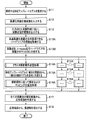
- FIG. 2 is a flowchart of the high-speed optimization device according to the first embodiment.
- the shape template model setting unit 30 of the high-speed optimization device 10 sets the shape template model 70 to be analyzed.
- the shape template model 70 may be input by the user, and the user may select any one of the shape template models 70 stored in the storage unit 12.
- the optimization problem definition unit 31 displays an input screen 40 shown in FIG. 5 to be described later, and acquires and defines an optimization problem definition variable 60 related to the shape template model 70, or the shape template Based on the model 70, one of the optimization problem definition variables 60 stored in the storage unit 12 is defined.
- the optimization problem definition variable 60 has an objective function, a constraint condition, a design variable, an experiment design method designation, and an experiment point designation.
- step S13 the experiment plan execution unit 32 outputs the experiment point design variable 61 based on the designation of the experiment design method and the designation of the number of experiment points input in step S12.
- step S ⁇ b> 14 the analysis order determination unit 33 performs an analysis order determination process based on the experiment point design variable 61 and outputs an analysis order determined experimental point group 62.
- step S15 the analysis model creation unit 34 creates the first analysis model 71-1 from the shape template model 70 and the first experimental point.
- step S ⁇ b> 16 the analysis execution unit 35 and the analysis result mapping execution unit 36 perform analysis and mapping processing according to the analysis order, and output an analysis result 80.
- step S ⁇ b> 17 the response surface construction unit 37 outputs a response surface 81 from the analysis results 80 of all experimental points.
- step S18 the optimization execution unit 38 outputs the optimal solution 82 from the response curved surface 81, and ends the process of FIG.
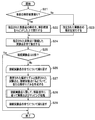
- FIG. 3 is a flowchart showing the analysis and mapping process according to the first embodiment. This analysis and mapping process is called in the process of step S16 in FIG. 2 and recursively called in the process of step S28 in FIG.
- step S21 the high-speed optimization device 10 determines whether there is a prior analysis result 80 or not. If there is a prior analysis result 80 (Yes), the process of step S22 is performed. If there is no prior analysis result 80 (No), the process of step S23 is performed.
- step S22 the analysis result mapping execution unit 36 maps the previous analysis result 80 to the analysis model 71 related to the designated experimental point.
- the analysis execution unit 35 executes numerical analysis based on the analysis model 71.
- step S23 the analysis execution unit 35 executes numerical analysis based on the analysis model 71 relating to the designated experimental point.
- step S24 the analysis result mapping execution unit 36 extracts all the experimental points connected to the designated experimental point.
- an experimental point connected to a designated experimental point is referred to as a “connection experimental point”.
- step S25 the analysis result mapping execution unit 36 determines whether the number of connection experiment points is zero. If the number of connection experiment points is zero (Yes), the processing in FIG. 3 is terminated. If the number of connection experiment points is not zero (No), the process of step S26 is performed. In steps S26 to S29, the analysis result mapping execution unit 36 repeats the process for all connection experiment points.
- step S27 the analysis result mapping execution unit 36 newly creates the next analysis model 71-n based on the specified analysis model 71, the specified experiment point, and the connection experiment point.
- step S28 the analysis result mapping execution unit 36 recursively calls the analysis and mapping process shown in FIG.
- step S29 if the analysis result mapping execution unit 36 repeats the process for all connection experiment points, the process of FIG. 3 ends.
- FIG. 4 is a diagram illustrating an example of a shape model of a bent tube with guide according to the first embodiment.
- the shape template model 70 of the curved pipe with guide is the shape template model 70 to be optimized in the first embodiment, and is stored in the storage unit 12.
- FIG. 4 shows an example in which the shape template model 70 is displayed in three dimensions.
- the cross section of the flow path of the bent pipe is rectangular and has an inlet 70a at the upper end.
- the flow path is directed downward from the inflow port 70a by the vertical rectangular flow path 70b, bent 90 degrees to the right side by the bend portion 70c, and directed to the right end outlet 70f through the horizontal rectangular flow path 70e.
- a guide 70d is provided in the bend portion 70c.
- the design variables in this embodiment are the radius R and the angle ⁇ .
- the radius R is the radius of the bend portion 70c of the flow path.
- the angle ⁇ is an angle with respect to the horizontal direction of the channel guide 70d.
- the objective function in the present embodiment is a function for calculating the total pressure loss coefficient V between the inlet 70a and the outlet 70f.
- the optimization problem according to the present embodiment is a problem of minimizing the value of the objective function by manipulating the design variable R and the design variable ⁇ .
- FIG. 5 is a diagram illustrating an example of an optimization problem definition input screen according to the first embodiment.
- the input screen 40 is displayed on the display 21 by the optimization problem definition unit 31, and information can be input by the keyboard 22 and the mouse 23.
- the input screen 40 is a window or dialog displayed by the application.
- the input screen 40 includes a title bar 41, an objective function input unit 42, a constraint condition input unit 43, a design variable input unit 44, an experiment design method input unit 45, an experiment score input unit 46, and execution of an experiment plan.
- a button 47 and a cancel button 48 are provided.
- the optimization problem definition variable 60 is input through the input screen 40. Based on the variables input to the design variable input unit 44, the experiment design method input unit 45, and the experiment point number input unit 46, the experiment point design variable 61 is output.
- the title bar 41 is displayed with a predetermined width at the upper end of the input screen 40, and the input screen 40 can be moved to a predetermined display location on the display 21 by dragging the mouse 23.
- “optimization problem definition” indicating the title of the input screen 40 and the name “guided curved pipe” of the shape template model 70 handled in this optimization are displayed.
- the objective function input unit 42 is disposed below the title bar 41, and includes an objective function selection unit 42a and a maximization / minimization selection unit 42b.
- the objective function selection unit 42a is a combo box, and has an area for displaying the currently selected item and a menu display area provided on the right side of this area. When this menu display area is clicked with the mouse 23, selectable items are displayed in a pull-down manner.
- the operation of the combo box is the same in the maximization / minimization selection unit 42b, the constraint condition input unit 43, and the experiment design method input unit 45 which are similarly configured by the combo box.
- the objective function selection unit 42a is a part that specifies an objective function that is an evaluation index to be optimized.
- the maximization / minimization selection unit 42b is a part that specifies whether to maximize or minimize the objective function designated by the objective function selection unit 42a.
- the designation of the objective function selection unit 42a and the designation of the maximization / minimization selection unit 42b can be a plurality of combinations.
- the constraint condition input unit 43 is a combo box arranged below the objective function input unit 42, and is a part that specifies the presence or absence of the constraint condition of the evaluation index. Further, when any evaluation index has a constraint condition, a part for specifying the type of the evaluation index related to the constraint condition and the allowable range of the evaluation index is newly displayed.
- the design variable input unit 44 is arranged on the lower side of the constraint condition input unit 43, and includes a character string “R [cm]” indicating a radius R as a design variable and “ ⁇ [degree]” indicating an angle ⁇ . Is placed on the left. On the right side of them, a character string “minimum value”, a minimum value input unit 44a-1 for inputting the minimum value of the radius R, and a minimum value input unit 44a-2 for specifying the minimum value of the angle ⁇ are arranged. Has been.
- a character string of “maximum value” for inputting the maximum value of the radius R, and a maximum value input unit 44b-2 for inputting the maximum value of the angle ⁇ .
- the name and number of design variables vary depending on the selected shape template model 70. The user can designate a range of design variables for performing an experiment design by inputting a minimum value and a maximum value of each design variable.
- the experiment design method input unit 45 is a combo box, and is a part for selecting the type of the experiment design method for determining the experiment point.
- the experimental score input unit 46 is a part for inputting the number of experimental points. In FIG. 5, Latin Hypercube Sampling (Latin superlattice method) is selected.
- the experiment plan execution button 47 is a button having a function of executing an experiment plan based on the input information.
- the cancel button 48 is a button having a function of canceling the experiment plan by discarding the input information.
- FIGS. 6A and 6B are diagrams showing examples of experimental point groups according to the first embodiment.
- FIG. 6B shows a plurality of numerical values included in the experimental point design variable 61.
- FIG. 6 shows an example of a result obtained by executing an experiment design method of Latin Hypercube Sampling (Latin superlattice method).
- the experimental point design variable 61 shown in FIG. 6 (a) has 10 records, each having items of ID, radius R, and angle ⁇ .
- the unit system of the numerical value of the radius R is centimeter [cm].
- the unit system of the numerical value of the angle ⁇ is degrees.
- FIG. 6B shows each experimental point related to the experimental point design variable 61 in a circle in the design variable space composed of the vertical axis ⁇ and the horizontal axis R.
- FIG. 6B is a diagram in which each experimental point is arranged in a two-dimensional design variable space based on the numerical value of each experimental point related to the experimental point design variable 61 shown in FIG.
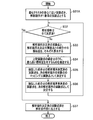
- FIG. 7 is a flowchart showing the analysis order determination process according to the first embodiment.
- the analysis order determination unit 33 sets the experimental point closest to the center in all design variables as the first experimental point in the analysis order.
- step S32 the analysis order determination unit 33 determines whether all the analysis orders of the experimental point design variables 61 have been determined. If all have been determined (Yes), the process of step S37 is performed. If not all have been determined (No), the process of step S33 is performed.
- step S ⁇ b> 33 the analysis order determination unit 33 calculates the similarity of the combination of the experiment point for which the analysis order has been determined and the experiment point for which the analysis order has not been determined. The calculation of the similarity is performed based on Formula 1 described later.
- step S ⁇ b> 34 the analysis order determination unit 33 extracts a combination having the highest similarity from the combination of the experimental points.
- step S ⁇ b> 35 the analysis order determination unit 33 determines the analysis point for which the analysis order of the extracted combination has been determined as a mapping source experimental point for the experiment point of the next analysis order.
- step S36 the analysis order determination unit 33 determines the extracted experimental point of the combination that has not been determined as the experimental point of the next analysis order, and returns to the process of step S32.
- step S37 the analysis order determination unit 33 outputs the analysis order determined experimental point group 62 to the analysis execution unit, and ends the process of FIG.
- This equation 1 squares the distance between the design variables of two experimental points in a predetermined design variable space, normalized by the range (difference between the maximum value and the minimum value) of the predetermined design variable space, Is a formula for subtracting the squared value and multiplying by a weighted value for each design variable, and calculating the similarity by the square root of the sum of the multiplied values.
- S in Formula 1 is a similarity, and it shows that it is similar, so that a value is large.
- Smp1 and smp2 in Equation 1 are identifiers that identify two experimental points that are targets of similarity calculation.
- Ci in Equation 1 represents a weighting factor for the similarity in design variable identifier i.
- C1 represents a weighting factor for the radius R
- C2 represents a weighting factor for the angle ⁇ .
- the weighting factor Ci for the similarity is set.
- the angle ⁇ is a design variable that controls the angle of the guide 70d.
- the angle ⁇ which is a design variable, affects the separation from the bend portion 70c to the outlet side and the separation itself that occurs at the lower portion of the guide 70d. Therefore, it is assumed that the angle ⁇ has a greater influence on the total pressure loss coefficient V that is an objective function than the radius R that is a design variable. Therefore, in this embodiment, the weighting coefficient C2 for the similarity of the design variable ⁇ is 2.0, and the weighting coefficient C1 for the similarity of the design variable R is 1.0.
- Equation 1 calculates the range of a predetermined design variable space by calculating the difference between the maximum value Xmax, i and the minimum value Xmin, i, and calculates the design variable distance between two experimental points within the range of the predetermined design variable space. It is normalized by dividing.
- Xsmp1, i and Xsmp2, i in Equation 1 are design variable values specified by the design variable identifier i in the experiment point identifiers smp1 and smp2, respectively.
- the design variable distance between two experimental points is obtained by the difference between the design variable value Xsmp1, i at one experimental point and the design variable value Xsmp2, i at the other experimental point.
- FIGS. 8A and 8B are diagrams showing an analysis order determination process (part 1) according to the first embodiment.
- FIG. 8A shows a method for determining the experimental point closest to the center.
- FIG. 8A shows the ID of an experimental point, the value of the design variable R of the experimental point, the value of the design variable ⁇ , the normalized coordinates of R, the normalized coordinates of ⁇ , and these normalized coordinates. And the distance from the center of the design variable space.
- FIG. 8B shows the result of the process in step S31 (FIG. 7) in which the experimental point closest to the center is the first experimental point in the analysis order among the experimental points shown in FIG. 6B.
- FIGS. 9A and 9B are diagrams illustrating an analysis order determination process (part 2) according to the first embodiment.
- FIG. 9 (b) shows the result of the first processing of steps S33 to S36 (FIG. 7) for the experimental point shown in FIG. 8 (b).
- FIGS. 10A to 10C are diagrams showing an analysis order determination process (part 3) according to the first embodiment.
- FIG. 10 (c) shows the result of the second processing of steps S33 to S36 (FIG. 7) for the experimental point shown in FIG. 9 (b).
- FIGS. 11A and 11B are diagrams illustrating examples of analysis order-determined experimental point groups according to the first embodiment.
- FIG. 11A shows numerical values of the analysis order determined experimental point group 62. This numerical value indicates the analysis order, the ID of the experimental point, the ID of the experimental point of the analysis mapping source, the value of the design variable R related to the experimental point, and the value of the design variable ⁇ related to the experimental point. ing.
- FIG. 11B shows a state in which all analysis orders have been determined by the analysis order determination process shown in FIG.
- “4” to “10” indicating the fourth to tenth are displayed on the circles indicating the fourth to tenth experimental points. is doing.
- the next experimental point to be analyzed based on a predetermined experimental point is indicated by an arrow.
- the analysis model creation unit 34 is a straight / planar shape of the shape model 70M-1, a curve / curved surface defined by a weighting factor of a polynomial, a Bezier / curved surface, a NURBS (non-uniform rational B-spline) curve. / Mesh is created for curved surface shape, and analysis model 71-1 is created.
- the analysis model creation unit 34 of this embodiment creates an analysis model 71-1 using a conventional mesh such as a tetrahedron or a hexahedron.
- a conventional mesh such as a tetrahedron or a hexahedron.
- the present invention is not limited to this, and the analysis model 71-1 may be created using any mesh as long as mapping of the analysis result 80 described later can be used.
- the analysis model 71-1 shown in FIG. 12C is applied to the boundary condition included in the optimization problem definition variable 60 based on the analysis model 71-1 shown in FIG. Analysis conditions are set based on this.
- the analysis model 71-1 of this embodiment shows that the fluid inflow condition 71in is set on the upper surface and the fluid outflow condition 71out is set on the right side surface.
- the present invention is not limited to this, and in the case of fluid analysis, it is possible to set a symmetry plane in addition to inflow conditions and outflow conditions. In the case of structural analysis, it is possible to set constraint conditions and load conditions.
- a mesh is created based on the shape model 70M-2, similarly to the analysis model 71-1 shown in FIG.
- the analysis execution unit 35 receives the analysis model 71-1 related to the experimental points included in the analysis order determined experimental point group 62 and the next analysis model 71-1 output by the analysis result mapping execution unit 36 described later. Used for numerical analysis such as fluid analysis and structural analysis.
- the analysis execution unit 35 analyzes the analysis model 71-1 related to the first experimental point in the analysis order determined experimental point group 62, there is no prior analysis result 80, and the analysis result 80 cannot be mapped. Numerical analysis from conditions.
- the analysis execution unit 35 analyzes the analysis model 71-n related to the second and subsequent experiment points in the analysis order determined experiment point group 62, the analysis result 80 in advance is mapped.
- the mapping of the analysis result 80 is that the element of the original convergence solution of the analysis result 80 is mapped to the element of the analysis model 71-n, and the flow velocity and density of the analysis result 80 are compared to the nodes of the analysis model 71-n. This refers to mapping physical quantities such as stress.
- mapping the analysis result 80 relating to the mapping source experiment point having a high degree of similarity to the analysis model 71-n it is possible to speed up the convergence of the numerical analysis relating to the new experiment point.
- the analysis execution unit 35 outputs an analysis result 80 when the numerical analysis has converged.
- the analysis execution unit 35 may map the analysis result 80 of another experimental point having a high degree of similarity and execute the analysis again when an error such as the numerical analysis diverges occurs. Similarly to the analysis model 71-1, the analysis may be performed from the initial condition.
- the analysis result mapping execution unit 36 maps the previous analysis result 80 to the analysis model 71-n of the next experimental point to be analyzed based on the analysis result 80.
- the information to be mapped is information for each element and node obtained by numerical analysis such as flow velocity, density, pressure, and stress.
- the mapping of the analysis result 80 specifies the closest element or node in the analysis model 71 that is the mapping source of the analysis result 80 with respect to all the elements or nodes in the analysis model 71-n of the experimental point to be analyzed next. Copy or interpolate the information to be mapped.
- the present invention is not limited to this, and the analysis result 80 may be mapped by a mesh morphing technique described in Patent Document 1.
- the physical quantity included in the information to be mapped may be averaged and mapped. Thereby, it is possible to stabilize numerical analysis.
- the analysis execution unit 35 When the analysis process starts, the analysis execution unit 35 performs a numerical analysis of the analysis model 71-1 from the initial conditions, and obtains an analysis result 80.
- the analysis result mapping execution unit 36 maps the analysis result 80 by the analysis model 71-1 to the analysis model 71-2 at the next experimental point.
- the analysis execution unit 35 starts numerical analysis of the analysis model 71-2 from a state in which the analysis result 80 is mapped in advance. Thereby, it is possible to obtain the analysis result 80 by reducing the time required for the numerical analysis as compared with the case of performing the numerical analysis from the initial condition where the analysis result 80 is not mapped. Thereafter, the analysis result mapping execution unit 36 repeats the process of mapping the analysis result 80 relating to the already analyzed experimental point to the analysis model 71-n of the next experimental point, and acquires all the analysis results 80.
- the response surface construction unit 37 uses the analysis result 80 obtained as a result of performing a numerical analysis on the analysis model 71 created using the experimental point design variable 61 and the information to be optimized using the information on the experimental point design variable 61.
- a response surface 81 related to the objective function of the index is constructed.
- any method of Kriging method, Radial Basis Function method, polynomial approximation, neural network, etc. may be used.
- the response surface construction unit 37 outputs the constructed response surface 81 to the optimization execution unit 38.
- FIGS. 14A and 14B are diagrams illustrating examples of response surfaces according to the first embodiment.
- FIG. 14A shows the relationship among the ID of each experimental point, the radius R, the angle ⁇ , and the value obtained by calculating the total pressure loss coefficient V, which is an objective function.
- FIG. 14 (b) shows a response surface 81 obtained by the Kriging method from the relationship between the total pressure loss coefficient V, the radius R, and the angle ⁇ shown in FIG. 14 (a).
- the lower right direction in FIG. 14B indicates the radius R
- the upper right direction in FIG. 14B indicates the angle ⁇
- the height direction in FIG. 14B indicates the total pressure loss coefficient V that is an evaluation index. Show.
- the response surface construction unit 37 of this embodiment calculates the response surface 81 by the Kriging method based on the values shown in FIG.
- the optimization execution unit 38 searches for a solution of an optimization problem based on the response surface 81 constructed by the response surface construction unit 37 and outputs an optimum solution 82.
- the optimum solution 82 is the coordinates of the design variable indicating the optimum value of the response surface 81.
- the optimization execution unit 38 can use, for example, a steepest descent method, a conjugate gradient method, an annealing method, a genetic algorithm, a particle swarm optimization (particle swarm optimization) method, etc. to solve the optimization problem. This makes it possible to solve optimization problems in numerical analysis such as fluid analysis and structural analysis at high speed.
- the first embodiment described above has the following effects (A) and (B).
- FIG. 15 is a schematic configuration diagram illustrating a high-speed optimization device according to the second embodiment. Elements common to the elements in FIG. 1 showing the first embodiment are denoted by common reference numerals.
- the high-speed optimization device 10A includes a clustering execution unit 39 in addition to the high-speed optimization device 10 according to the first embodiment. Further, a plurality of experiment point design variables 61, a plurality of analysis order determined experiment point groups 62, a plurality of analysis models 71-1, a plurality of analysis results 80, and a plurality of next analysis models 71-n. Have.
- the clustering execution unit 39 performs a clustering execution process for clustering (dividing) the experiment point design variable 61 output by the experiment plan execution unit 32 by the k-means method (K-means method).
- the analysis order design variable 61 that has been clustered has its analysis order determined in parallel by the analysis order determination unit 33 and becomes a clustered analysis order determined experimental point group 62.
- the analysis model creation unit 34, the analysis execution unit 35, and the analysis result mapping execution unit 36 can obtain the analysis result 80 at higher speed by processing the information for each cluster in parallel. .
- FIG. 16 is a flowchart of the high-speed optimization device according to the second embodiment. Elements common to the elements in FIG. 2 showing the first embodiment are denoted by common reference numerals.
- the processing in steps S11 to S13 is the same as the processing in FIG. 2 showing the first embodiment.
- the clustering execution unit 39 acquires the number of pieces of hardware that can be processed in parallel in the high-speed optimization device 10A.
- the number of hardware that can be processed in parallel is the number of execution units (cores) in a multi-core processor, the number of processors in a symmetric multiprocessor, and the number of processing nodes in a distributed computer.
- step S13B the experimental points of the experimental point design variable 61 are divided into clusters corresponding to the number of hardware by the k-means method (K average method).
- the processing in steps S14A to S16A is parallel processing for the number of hardware.
- step S14A as in step S14 shown in FIG. 2, processing for determining the cluster analysis order is performed in parallel on the experimental points of each cluster.
- step S15A as in step S15 shown in FIG. 2, the first analysis model 71-1 in each cluster is created in parallel from the shape template model 70 and the first experimental point in each cluster.
- step S16A similarly to step S16 shown in FIG. 2, analysis and mapping processing are performed in parallel according to the analysis order. If the parallel processing in step S16A has been completed for all hardware capable of parallel processing, the processing in step S17 is performed. Further, the processing of steps S17 to S18 is performed in the same manner as the processing of FIG. 2 showing the first embodiment, and an optimal solution 82 is obtained.
- FIG. 17 is a flowchart showing an analysis order determination process according to the second embodiment. Elements common to the elements in FIG. 7 showing the first embodiment are denoted by common reference numerals.
- step S31A the experimental point closest to the center of gravity of the cluster is set as the first experimental point in the analysis order. Further, the processing of steps S32 to S37 is performed in the same manner as the processing of FIG. 7 showing the first embodiment, and the analysis order determined experimental point group 62 for each cluster is output.
- the second embodiment described above has the following effects (C) and (D).
- C Since the experimental points are divided into clusters and processed in parallel for each cluster, it is possible to shorten the processing time of the analysis execution unit 35 having the largest processing amount.
- D The number of pieces of hardware that can be processed in parallel is acquired in advance, and the experimental points are divided into clusters according to the number of pieces of hardware, so that the effect of shortening the processing time by parallel processing is the highest.
- the high-speed optimization device 10 according to the third embodiment has the same configuration as that of the high-speed optimization device 10 according to the first embodiment.
- FIG. 18 is a flowchart showing analysis and mapping processing according to the third embodiment. Elements common to the elements in FIG. 3 showing the first embodiment are denoted by common reference numerals.
- the processes in steps S21 to S25 are the same as the processes in steps S21 to S25 of FIG. 3 showing the first embodiment.
- the processing in steps S27A to S28A is parallel processing for the number of connection experiment points.
- the analysis result mapping execution unit 36 newly sets the next analysis model 71-n for each connection experiment point based on the designated analysis model 71, the designated experiment point, and the connection experiment point. Create in parallel.
- step S28A the analysis result mapping execution unit 36 recursively calls the analysis and mapping parallel processing shown in FIG. When all the parallel processing in step S28A is completed, the processing in FIG. 18 is terminated.
- the high-speed optimization devices 10 and 10A are configured.
- the present invention is not limited to this, and may be configured as a high-speed optimization program that operates on a computer.
- the experiment plan execution unit 32 calculates the similarity between two experiment points using the function shown in Equation 1.
- the present invention is not limited to this.
- a function that is calculated based on any one of the Euclidean distance, the standard Euclidean distance, the Mahalanobis distance, the Manhattan distance, the Chebyshev distance, and the Minkowski distance between the two experimental points may be used.
- values obtained by these functions may be converted by a predetermined function to calculate a similarity.
- the experimental point design variable 61 is divided into clusters by the k-means method (K-means method).
- K-means method the k-means method
- the present invention is not limited to this, and the experimental point design variable 61 is converted into a cluster by the shortest distance method, longest distance method, median method, center of gravity method, group average method, Ward method, variable method, and self-organizing map (Kohonen network). It may be divided.
- the weighting factor C2 for the similarity of the design variable ⁇ and the weighting factor C1 for the similarity of the design variable R are determined based on the appearance of the shape template model 70.
- the present invention is not limited to this, and the optimization problem is analyzed by setting all the weighting factors to 1.0, the response surface 81 is output, and the slope (sensitivity) for each design variable of the response surface 81 is designed. Integration may be performed over the entire variable space, and a weighting coefficient may be set in accordance with the integrated slope (sensitivity). As a result, the most appropriate weighting factor can be set for each design variable, and the optimization problem can be analyzed at high speed.
- (F) In 3rd Embodiment it processes in parallel for every number of connection experiment points.
- the present invention is not limited to this, and the number of parallel processes for all connection experiment points operating in the high-speed optimization device 10 is managed, and the number of parallel processes is a predetermined number (for example, the number of hardware capable of parallel processing Etc.), as shown in FIG. 3, the process may be switched to a process that is repeated for all connection test points.
- the process may be switched to a process that is repeated for all connection test points.
Landscapes
- Engineering & Computer Science (AREA)
- Physics & Mathematics (AREA)
- Theoretical Computer Science (AREA)
- Computer Hardware Design (AREA)
- Evolutionary Computation (AREA)
- Geometry (AREA)
- General Engineering & Computer Science (AREA)
- General Physics & Mathematics (AREA)
- Management, Administration, Business Operations System, And Electronic Commerce (AREA)
Abstract
【課題】 解析結果のデータベース無しに、既に解析された解析結果を活用し、高速で構造解析や流体解析を行う。 【解決手段】 高速最適化装置10は、3次元CADデータの形状テンプレートモデル70の所定の設計変数空間に係る数値解析により最適解82を求める。設計変数空間における実験点の類似度に基づいて、複数の実験点の解析順序を決定し、解析順序決定済実験点群62を出力する。この解析順序決定済実験点群62の1番目の実験点と形状テンプレートモデル70に係る設計変数に基づき、1番目の解析モデル71-1を作成する。更に、所定の実験点に基づいて解析モデル71を解析して解析結果80を出力し、次の実験点に係る解析モデル71-nに解析結果80をマッピングする処理を、すべての解析順序決定済実験点群62について繰り返す。
Description
本発明は、CAD(Computer Aided Design=コンピュータ支援設計)/CAM(computer aided manufacturing=コンピュータ支援製造)用データの数値解析に要する時間を最適化する高速最適化装置、およびプログラムに関する。
従来の製品設計では、実機の試作品を作成し、流体解析や構造解析などの数値解析によって評価していた。しかし、この実機による評価には多くの時間と工数を要する欠点がある。近年、試作品のCAD/CAM用データを、流体解析や構造解析などの数値解析によって評価し、実機による評価回数を減らす試みが行われている。
特許文献1には、数値流体計算により目標とする評価指標を満足する給気ポートの最適形状を求める設計支援装置において、新たに解析を行おうとする新規の設計変数と、既に解析が行われた過去の設計変数とが類似するか否かを判定し、評価指標の解析結果が流れの剥離を伴うものであるか否かを判定し、更に、新規の設計変数と過去の設計変数とが類似していると判定された場合に、当該新規の設計変数に対する評価指標の解析結果として、当該新規の設計変数と類似し、かつ、剥離を伴わない過去の設計変数に対する評価指標の解析結果を割り当て、給気ポートの最適形状を高速に求める技術が開示されている。
特許文献1に記載の発明は、解析時間の短縮に有効である。しかし、既に解析済みの解析モデルと、その解析結果が十分に格納された解析結果データベースとを要する、という課題がある。
そこで、本発明の目的は、解析結果データベースが存在しない場合であっても、効率よく解析時間を短縮する手法を提供することを課題とする。
そこで、本発明の目的は、解析結果データベースが存在しない場合であっても、効率よく解析時間を短縮する手法を提供することを課題とする。
前記課題を解決し、本発明の目的を達成するために、以下のように構成した。
すなわち、本発明の高速最適化装置は、3次元CAD(Computer Aided Design)データの形状テンプレートモデルの所定の設計変数空間に係る数値解析を行い、最適解を求める高速最適化装置であって、前記所定の設計変数空間における複数の実験点の解析順序を決定し、解析順序決定済実験点群を出力する解析順序決定部と、前記形状テンプレートモデルと1番目の実験点に係る設計変数情報に基づき、1番目の解析モデルを作成する解析モデル作成部と、解析モデルを解析し、解析結果を出力する解析実行部と、前記解析順序決定済実験点群において、解析モデルに係る所定の実験点に基づく次の実験点が有る場合には、前記所定の実験点に係る解析結果を、前記次の実験点に係る解析モデルにマッピングする解析結果マッピング実行部とを備えたことを特徴とする。
本発明の高速最適化プログラムは、3次元CAD(Computer Aided Design)データの形状テンプレートモデルの所定の設計変数空間に係る数値解析をコンピュータに行わせ、最適解をコンピュータに求めさせる高速最適化プログラムであって、前記所定の設計変数空間における複数の実験点の解析順序を決定し、解析順序決定済実験点群を出力する解析順序決定処理と、前記形状テンプレートモデルと1番目の実験点に係る設計変数情報に基づき、1番目の解析モデルを作成する解析モデル作成処理と、解析モデルを解析し、解析結果を出力する解析実行処理と、前記解析順序決定済実験点群において、解析モデルに係る所定の実験点に基づく次の実験点が有る場合には、前記所定の実験点に係る解析結果を、前記次の実験点に係る解析モデルにマッピングする解析結果マッピング実行処理とコンピュータに行わせる。
その他の手段については、発明を実施するための形態のなかで説明する。
その他の手段については、発明を実施するための形態のなかで説明する。
本発明によれば、解析結果データベースが存在しない場合であっても,実験点の解析に必要な時間を効率よく短縮する、いわゆる処理時間の最適化を行うことが可能となる。
以降、本発明を実施するための形態(「本実施形態」という)を、図等を参照して詳細に説明する。
(第1の実施形態)
図1は、第1の実施形態に係る高速最適化装置を示す概略の構成図である。
高速最適化装置10は,制御部11と、記憶部12と、入出力部20と、形状テンプレートモデル設定部30と、最適化問題定義部31と、実験計画実行部32と、解析順序決定部33と、解析モデル作成部34と、解析実行部35と、解析結果マッピング実行部36と、応答曲面構築部37と、最適化実行部38とを備えている。
制御部11は、この高速最適化装置10全体の動作を統括する機能を有している。
図1は、第1の実施形態に係る高速最適化装置を示す概略の構成図である。
高速最適化装置10は,制御部11と、記憶部12と、入出力部20と、形状テンプレートモデル設定部30と、最適化問題定義部31と、実験計画実行部32と、解析順序決定部33と、解析モデル作成部34と、解析実行部35と、解析結果マッピング実行部36と、応答曲面構築部37と、最適化実行部38とを備えている。
制御部11は、この高速最適化装置10全体の動作を統括する機能を有している。
記憶部12は、例えばハードディスクやフラッシュメモリなどの大容量記憶媒体であり、3次元CAD(Computer Aided Design)に係る複数の形状テンプレートモデル70と複数の最適化問題定義変数60とを記憶している。
入出力部20は、高速最適化装置10の使用者がデータを入力するためのキーボード22やマウス23と、入力したデータや記憶部12に格納されているデータを表示するためのディスプレイ21とを有している。
形状テンプレートモデル設定部30は、記憶部12に格納されている複数の形状テンプレートモデル70や、外部から入力された形状テンプレートモデル70を、入出力部20に表示させ、この表示した形状テンプレートモデル70のいずれかを選択して設定する機能を有している。
最適化問題定義部31は、設定された形状テンプレートモデル70に基づいて、この形状テンプレートモデル70に係る最適化問題定義の入力画面40(図5)を表示して最適化問題定義変数60を取得して定義するか、または、記憶部12に格納されている複数の最適化問題定義変数60のうちいずれかを選択して定義する最適化問題定義処理を行う。最適化問題定義変数60は、解析結果80の条件を規定する変数群であり、3次元CADデータの形状テンプレートモデル70を数値解析する種々の変数、例えば、目的関数、制約条件、所定の設計変数空間を示す設計変数とその設計変数の範囲、実験計画法の指定、実験点数の指定などを有している。
本実施形態における目的関数は、例えば、流体解析や構造解析などの数値解析の結果得られる圧力損失係数や応力と言った数値データなどである。
本実施形態における制約条件は、例えば、数値解析して得られる数値データに関する制約や、最適化対象となる形状の幾何的制約などである。
本実施形態における制約条件は、例えば、数値解析して得られる数値データに関する制約や、最適化対象となる形状の幾何的制約などである。
本実施形態における設計変数は、例えば、最適化対象となる形状を規定するための寸法や、形状を規定するために用いる曲線や、多項式の重み係数で定義される曲線/曲面形状や、ベジェ曲線/曲面形状や、NURBS(非一様有理Bスプライン)曲線/曲面形状や、曲面の制御点座標や重み係数や、解析モデル71(=71-1,71-n,…)に固有の解析条件である流速や圧力である。設計変数の範囲とは、それぞれの設計変数の最大値と最小値で規定される多次元の設計変数空間である。
実験計画法とは、ある結果(効果)をもたらす複数の要因が、互いに均等に作用しあう(直交するという)条件で、最小限の回数の実験により、効果を予測する手法のことである。本実施形態における実験計画法は、例えば直交表、中心複合計画、Latin Hypercube Sampling(ラテン超格子法)などである。
実験計画法とは、ある結果(効果)をもたらす複数の要因が、互いに均等に作用しあう(直交するという)条件で、最小限の回数の実験により、効果を予測する手法のことである。本実施形態における実験計画法は、例えば直交表、中心複合計画、Latin Hypercube Sampling(ラテン超格子法)などである。
実験計画実行部32は、最適化問題定義変数60が有している前記所定の設計変数空間から、最適解82の探索に用いる複数の実験点である実験点設計変数61を決定する機能を有している。
解析順序決定部33は、実験計画実行部32によって決定された複数の実験点である実験点設計変数61に基づいて、解析順序を決定し、解析順序決定済実験点群62を出力する解析順序決定処理を行う。
解析モデル作成部34は、形状テンプレートモデル70と所定の実験点に係る設計変数情報に基づき、1番目の解析モデル71-1を作成する解析モデル作成処理を行う。
解析実行部35は、解析モデル71を、この解析モデル71に係る所定の実験点の設計変数情報を用いて解析し、この所定の実験点に係る解析結果80を出力する解析実行処理を行う。
解析結果マッピング実行部36は、この所定の実験点に基づいて解析する次の実験点が有る場合には、この所定の実験点に係る解析結果80を、次の実験点に係る解析モデル71-n(nは2以上の自然数)にマッピングする解析結果マッピング実行処理を行う。
応答曲面構築部37は、全ての複数の実験点に係る解析結果80を用いて最適化問題における制約条件の応答曲面81を構築する応答曲面構築処理を行う。
最適化実行部38は、応答曲面構築部37によって出力された応答曲面81を用いて最適解82を算出する最適化実行処理を行う。
応答曲面構築部37は、全ての複数の実験点に係る解析結果80を用いて最適化問題における制約条件の応答曲面81を構築する応答曲面構築処理を行う。
最適化実行部38は、応答曲面構築部37によって出力された応答曲面81を用いて最適解82を算出する最適化実行処理を行う。
(第1の実施形態の動作)
図1を元に、高速最適化装置10の動作を説明する。
実験計画実行部32は、本装置使用者が入出力部20を使用して、本装置を用いて実行する最適化問題定義変数60を入力し、応答曲面81を構築するために必要な実験点を決定するため実験計画を実行し、実験点設計変数61を出力する。実験点設計変数61は、目的関数、制約条件、所定の設計変数空間を示す設計変数とその設計変数の範囲、実験計画法の指定、実験点数の指定などを有している。
図1を元に、高速最適化装置10の動作を説明する。
実験計画実行部32は、本装置使用者が入出力部20を使用して、本装置を用いて実行する最適化問題定義変数60を入力し、応答曲面81を構築するために必要な実験点を決定するため実験計画を実行し、実験点設計変数61を出力する。実験点設計変数61は、目的関数、制約条件、所定の設計変数空間を示す設計変数とその設計変数の範囲、実験計画法の指定、実験点数の指定などを有している。
図2は、第1の実施形態に係る高速最適化装置のフローチャートである。
処理が開始すると、ステップS11において、高速最適化装置10の形状テンプレートモデル設定部30は、解析する形状テンプレートモデル70を設定する。形状テンプレートモデル70は、ユーザが入力しても良く、さらに、記憶部12に格納されている形状テンプレートモデル70のいずれかをユーザが選択しても良い。
処理が開始すると、ステップS11において、高速最適化装置10の形状テンプレートモデル設定部30は、解析する形状テンプレートモデル70を設定する。形状テンプレートモデル70は、ユーザが入力しても良く、さらに、記憶部12に格納されている形状テンプレートモデル70のいずれかをユーザが選択しても良い。
ステップS12において、最適化問題定義部31は、後述する図5に示す入力画面40を表示して、形状テンプレートモデル70に係る最適化問題定義変数60を取得して定義するか、又は、形状テンプレートモデル70に基づいて、記憶部12に格納されている最適化問題定義変数60のうちいずれかを定義する。最適化問題定義変数60は、目的関数、制約条件、設計変数、実験計画法の指定、実験点数の指定を有している。
ステップS13において、実験計画実行部32は、ステップS12において入力された実験計画法の指定と、実験点数の指定とに基づいて、実験点設計変数61を出力する。
ステップS14において、解析順序決定部33は、実験点設計変数61に基づいて、解析順序決定処理を行い、解析順序決定済実験点群62を出力する。
ステップS15において、解析モデル作成部34は、形状テンプレートモデル70と1番目の実験点から、1番目の解析モデル71-1を作成する。
ステップS14において、解析順序決定部33は、実験点設計変数61に基づいて、解析順序決定処理を行い、解析順序決定済実験点群62を出力する。
ステップS15において、解析モデル作成部34は、形状テンプレートモデル70と1番目の実験点から、1番目の解析モデル71-1を作成する。
ステップS16において、解析実行部35と解析結果マッピング実行部36とは、解析順序に従って解析およびマッピング処理を行い、解析結果80を出力する。
ステップS17において、応答曲面構築部37は、全ての実験点の解析結果80から、応答曲面81を出力する。
ステップS18において、最適化実行部38は、応答曲面81から、最適解82を出力し、図2の処理を終了する。
ステップS17において、応答曲面構築部37は、全ての実験点の解析結果80から、応答曲面81を出力する。
ステップS18において、最適化実行部38は、応答曲面81から、最適解82を出力し、図2の処理を終了する。
図3は、第1の実施形態に係る解析およびマッピング処理を示すフローチャートである。この解析およびマッピング処理は、図2のステップS16の処理で呼び出されるほか、この図3のステップS28の処理で再帰的に呼び出される。
処理が開始すると、ステップS21において、高速最適化装置10は、事前の解析結果80が有るか否かを判断する。事前の解析結果80が有れば(Yes)、ステップS22の処理を行う。事前の解析結果80が無ければ(No)、ステップS23の処理を行う。
ステップS22において、解析結果マッピング実行部36は、指定された実験点に係る解析モデル71に事前の解析結果80をマッピングする。解析実行部35は、この解析モデル71に基づいて数値解析を実行する。
ステップS23において、解析実行部35は、指定された実験点に係る解析モデル71に基づいて数値解析を実行する。
ステップS23において、解析実行部35は、指定された実験点に係る解析モデル71に基づいて数値解析を実行する。
ステップS24において、解析結果マッピング実行部36は、指定された実験点に接続している実験点を全て抽出する。以下、指定された実験点に接続している実験点を「接続実験点」という。
ステップS25において、解析結果マッピング実行部36は、接続実験点が0個であるか否かを判断する。接続実験点が0個ならば(Yes)、図3の処理を終了する。接続実験点が0個でないならば(No)、ステップS26の処理を行う。
ステップS26~S29において、解析結果マッピング実行部36は、接続実験点の全てについて処理を繰り返す。
ステップS26~S29において、解析結果マッピング実行部36は、接続実験点の全てについて処理を繰り返す。
ステップS27において、解析結果マッピング実行部36は、指定された解析モデル71と指定された実験点と、接続実験点にもとづいて、新たに次の解析モデル71-nを作成する。
ステップS28において、解析結果マッピング実行部36は、この図3に示す解析およびマッピング処理を再帰的に呼び出す。
ステップS29において、解析結果マッピング実行部36は、全ての接続実験点について処理を繰り返したならば、図3の処理を終了する。
ステップS28において、解析結果マッピング実行部36は、この図3に示す解析およびマッピング処理を再帰的に呼び出す。
ステップS29において、解析結果マッピング実行部36は、全ての接続実験点について処理を繰り返したならば、図3の処理を終了する。
図4は、第1の実施形態に係るガイド付き曲がり管の形状モデルの例を示す図である。
ガイド付き曲がり管の形状テンプレートモデル70は、第1の実施形態における最適化対象の形状テンプレートモデル70であり、記憶部12に格納されている。図4は、この形状テンプレートモデル70を3次元で表示した例を示している。
ガイド付き曲がり管の形状テンプレートモデル70は、第1の実施形態における最適化対象の形状テンプレートモデル70であり、記憶部12に格納されている。図4は、この形状テンプレートモデル70を3次元で表示した例を示している。
この曲がり管の流路の断面は矩形であり、上端に流入口70aを有している。流路は、この流入口70aから、垂直の矩形流路70bによって下方向に向かい、ベンド部70cによって右側に90度湾曲し、水平の矩形流路70eを介して右端の流出口70fへと向かっている。更に、このベンド部70cには、ガイド70dが設けられている。
本実施形態における設計変数は、半径Rと角度θである。半径Rは、流路のベンド部70cの半径である。角度θは、流路のガイド70dの水平方向に対する角度である。
本実施形態における目的関数は、流入口70aから流出口70fまでの間の全圧損失係数Vを算出する関数である。本実施形態に係る最適化問題とは、設計変数Rと設計変数θとを操作して、この目的関数の値を最小化する問題である。
≪最適化問題定義部31の動作≫
図5は、第1の実施形態に係る最適化問題定義の入力画面の例を示す図である。
入力画面40は、最適化問題定義部31によってディスプレイ21に表示され、キーボード22およびマウス23によって情報の入力が可能である。入力画面40は、アプリケーションが表示するウインドウまたはダイアログである。
図5は、第1の実施形態に係る最適化問題定義の入力画面の例を示す図である。
入力画面40は、最適化問題定義部31によってディスプレイ21に表示され、キーボード22およびマウス23によって情報の入力が可能である。入力画面40は、アプリケーションが表示するウインドウまたはダイアログである。
入力画面40は、タイトルバー41と、目的関数入力部42と、制約条件入力部43と、設計変数入力部44と、実験計画法入力部45と、実験点数入力部46と、実験計画の実行ボタン47と、キャンセルボタン48とを備えている。
最適化問題定義変数60は、この入力画面40によって入力される。設計変数入力部44と、実験計画法入力部45と、実験点数入力部46とに入力された変数にもとづいて、実験点設計変数61が出力される。
最適化問題定義変数60は、この入力画面40によって入力される。設計変数入力部44と、実験計画法入力部45と、実験点数入力部46とに入力された変数にもとづいて、実験点設計変数61が出力される。
タイトルバー41は、この入力画面40の上端に所定の幅で表示されており、マウス23のドラッグによって、入力画面40をディスプレイ21の所定の表示場所に移動させることが可能である。タイトルバー41には、この入力画面40のタイトルを示す「最適化問題定義」と、この最適化で取り扱う形状テンプレートモデル70の名称「ガイド付き曲がり管」が表示されている。
目的関数入力部42は、タイトルバー41の下側に配置されており、目的関数選択部42aと、最大化/最小化選択部42bとを有している。目的関数選択部42aはコンボボックスであり、現在選択されている項目を表示する領域と、この領域の右側に設けられているメニュー表示領域とを有している。このメニュー表示領域をマウス23でクリックすることによって、選択可能な項目がプルダウン表示される。このコンボボックスの動作は、同様にコンボボックスによって構成されている最大化/最小化選択部42bと制約条件入力部43と実験計画法入力部45においても同様である。
目的関数選択部42aは、最適化する評価指標となる目的関数を指定する部位である。最大化/最小化選択部42bは、目的関数選択部42aによって指定した目的関数を最大化するか最小化するかを指定する部位である。目的関数選択部42aの指定と、最大化/最小化選択部42bの指定は、複数の組合せが可能である。
制約条件入力部43は、目的関数入力部42の下側に配置されているコンボボックスであり、評価指標の制約条件の有無を指定する部位である。更に、いずれかの評価指標が制約条件を有する場合には、制約条件に係る評価指標の種別と、その評価指標の許容範囲とを指定する部位が新たに表示される。
設計変数入力部44は、制約条件入力部43の下側に配置されており、設計変数である半径Rを示す「R[cm]」の文字列と、角度θを示す「θ[degree]」の文字列が左側に配置されている。それらの右側には、「最小値」の文字列と、半径Rの最小値を入力する最小値入力部44a-1と、角度θの最小値を指定する最小値入力部44a-2とが配置されている。更にそれらの右側には、「最大値」の文字列と、半径Rの最大値を入力する最大値入力部44b-1と、角度θの最大値を入力する最大値入力部44b-2とが配置されている。各設計変数の名称と個数とは、選択された形状テンプレートモデル70に依存して変動する。ユーザは、各設計変数の最小値と最大値とを入力することによって、実験計画を行う設計変数の範囲を指定することが可能である。
実験計画法入力部45は、コンボボックスであり、実験点を決定する実験計画法の種別を選択する部位である。実験点数入力部46は、実験点の個数を入力する部位である。図5では、Latin Hypercube Sampling(ラテン超格子法)が選択されている。
実験計画の実行ボタン47は 入力した情報に基づいて、実験計画を実行する機能を有するボタンである。キャンセルボタン48は、入力した情報を破棄して、実験計画をキャンセルする機能を有するボタンである。
≪実験計画実行部32の動作≫
入力画面40に全ての情報を入力し、実験計画の実行ボタン47をクリックすると、実験計画実行部32によって指定された実験計画法が実行され、実験点設計変数61が出力される。
入力画面40に全ての情報を入力し、実験計画の実行ボタン47をクリックすると、実験計画実行部32によって指定された実験計画法が実行され、実験点設計変数61が出力される。
図6(a),(b)は、第1の実施形態に係る実験点群の例を示す図である。図6(a)は実験点設計変数61が有している複数の実験点(ID=1~10)の数値を示し、図6(b)は実験点設計変数61が有している複数の実験点(ID=1~10)の設計変数空間上の配置を示している。図6は、Latin Hypercube Sampling(ラテン超格子法)の実験計画法が実行された結果の例を示している。
図6(a)に示す実験点設計変数61は、10個のレコードを有しており、それぞれIDと、半径Rと、角度θの項目を有している。半径Rの数値の単位系はセンチメートル[cm]である。角度θの数値の単位系は度[degree]である。例えば、ID=1の実験点は、形状テンプレートモデル70(図4)に基づいて、半径R=0.525cm、角度θ=52.5度とした解析モデル71に対応していることを示している。
図6(b)は、縦軸θと横軸Rとで構成される設計変数空間において、実験点設計変数61に係る各実験点を丸印で示している。図6(b)は、図6(a)に示す実験点設計変数61に係る各実験点の数値に基づいて、2次元の設計変数空間に各実験点を配置したものである。例えば、ID=1の実験点は、半径R=0.525cm、角度θ=52.5度であることを示している。
入力画面40(図5)で最適化問題定義変数60を設定し、この設定した最適化問題定義変数60に従って実験計画を行うことにより、上述した図6(a),(b)に示す実験点設計変数61を決定することが可能である。
実験点設計変数61は、実験点ごとの設計変数の組み合わせを格納している。
≪解析順序決定部33の動作≫
図7は、第1の実施形態に係る解析順序決定処理を示すフローチャートである。
処理が開始すると、ステップS31において、解析順序決定部33は、全設計変数において最も中心に近い実験点を、解析順序が1番目の実験点とする。
実験点設計変数61は、実験点ごとの設計変数の組み合わせを格納している。
≪解析順序決定部33の動作≫
図7は、第1の実施形態に係る解析順序決定処理を示すフローチャートである。
処理が開始すると、ステップS31において、解析順序決定部33は、全設計変数において最も中心に近い実験点を、解析順序が1番目の実験点とする。
ステップS32において、解析順序決定部33は、実験点設計変数61の解析順序は全て決定済か否かを判断する。全て決定済であったならば(Yes)、ステップS37の処理を行う。全て決定済でなかったならば(No)、ステップS33の処理を行う。
ステップS33において、解析順序決定部33は、解析順序決定済の実験点と、解析順序未決定の実験点との組合せの類似度を、それぞれ算出する。この類似度の計算は、後述ずる数式1に基づいて行う。
ステップS34において、解析順序決定部33は、上記実験点の組合せのうち、最も高い類似度を有するものを抽出する。
ステップS35において、解析順序決定部33は、抽出した組合せの解析順序決定済の実験点を、次の解析順序の実験点のマッピング元実験点として決定する。
ステップS34において、解析順序決定部33は、上記実験点の組合せのうち、最も高い類似度を有するものを抽出する。
ステップS35において、解析順序決定部33は、抽出した組合せの解析順序決定済の実験点を、次の解析順序の実験点のマッピング元実験点として決定する。
ステップS36において、解析順序決定部33は、抽出した組合せの解析順序未決定の実験点を、次の解析順序の実験点として決定し、ステップS32の処理に戻る。
ステップS37において、解析順序決定部33は、解析順序決定済実験点群62を解析実行部に出力し、図7の処理を終了する。
ステップS37において、解析順序決定部33は、解析順序決定済実験点群62を解析実行部に出力し、図7の処理を終了する。

ここで、解析順序決定部33がステップS33において、類似度の計算を行う数式1について説明する。この数式1は、所定の設計変数空間における2つの実験点の設計変数の距離を、前記所定の設計変数空間の範囲(最大値と最小値との差)で正規化して自乗し、1.0から前記自乗した値を減算して設計変数ごとに重みづけした値を乗算し、前記乗算した値の総和の平方根によって類似度を算出する式である。
数式1中のSは、類似度であり、値が大きいほど類似していることを示している。
数式1中のsmp1、smp2は、類似度の算出対象である2つの実験点を識別する識別子である。
数式1中のSは、類似度であり、値が大きいほど類似していることを示している。
数式1中のsmp1、smp2は、類似度の算出対象である2つの実験点を識別する識別子である。
数式1中のndvは、設計変数の数を示し、iは、設計変数の識別子を示している。本実施形態の設計変数は、半径Rと角度θの2個なので、設計変数の数ndv=2である。
数式1中のCiは、設計変数の識別子iにおける類似度に対する重み係数を示している。本実施形態において、C1は半径Rの重み係数を示し、C2は角度θの重み係数を示している。この重み係数Ciにより、所定の設計変数空間における2つの実験点の類似度を、設計変数ごとに重みづけすることが可能である。この数式1の重み係数Ciにより、解析結果80に高い影響を及ぼす設計変数に対し、高い重みづけが可能となり、最適化問題の解析を短時間に収束させることが可能となる。
本実施形態では、設計変数によって目的関数に対する影響度合が異なることが考慮された上で、類似度に対する重み係数Ciが設定される。形状テンプレートモデル70(図4)の形状において、角度θは、ガイド70dの角度を制御する設計変数である。設計変数である角度θは、ベンド部70cから出口側にかけての剥離や、ガイド70dの下部に発生する剥離そのものに影響を及ぼす。よって、角度θは、設計変数である半径Rと比較して、目的関数である全圧損失係数Vに対する影響度合が大きいことが想定される。よって、本実施形態では、設計変数θの類似度に対する重み係数C2は2.0とし、設計変数Rの類似度に対する重み係数C1は1.0とする。
数式1中のXmax,i、Xmin,iは、それぞれ実験計画実行部32によって決定した設計変数識別子iにおける最大値と最小値を示している。数式1は、最大値Xmax,iと最小値Xmin,iの差を求めることによって所定の設計変数空間の範囲を求め、2つの実験点の設計変数距離を、この所定の設計変数空間の範囲で除算して正規化している。
数式1中のXsmp1,i、Xsmp2,iは、それぞれ実験点の識別子smp1、smp2における設計変数識別子iによって指定される設計変数の値である。数式1は、一方の実験点の設計変数の値Xsmp1,iと、他方の実験点の設計変数の値Xsmp2,iとの差によって、2つの実験点の設計変数距離を求めている。
図8(a),(b)は、第1の実施形態に係る解析順序決定処理(その1)を示す図である。
図8(a)は、最も中心に近い実験点の決定方法を示している。図8(a)は、実験点のIDと、その実験点の設計変数Rの値と、設計変数θの値と、Rの正規化座標と、θの正規化座標と、これらの正規化座標と設計変数空間の中心との距離を示している。更に、ID=10の実験点が、最も中心に近い実験点であることを示している。これは、図7に示すステップS31の処理に対応している。
図8(a)は、最も中心に近い実験点の決定方法を示している。図8(a)は、実験点のIDと、その実験点の設計変数Rの値と、設計変数θの値と、Rの正規化座標と、θの正規化座標と、これらの正規化座標と設計変数空間の中心との距離を示している。更に、ID=10の実験点が、最も中心に近い実験点であることを示している。これは、図7に示すステップS31の処理に対応している。
図8(b)は、図6(b)で示す実験点において、最も中心に近い実験点を解析順序が1番目の実験点とするステップS31(図7)の処理の結果を示している。図6(b)と同様な表示に加えて、1番目に決定したID=10の実験点を示す丸印に、1番目に決定した実験点を示す「1」を表示している。
図9(a),(b)は、第1の実施形態に係る解析順序決定処理(その2)を示す図である。
図9(a),(b)は、第1の実施形態に係る解析順序決定処理(その2)を示す図である。
図9(a)は、1回目のステップS33(図7)の処理の結果の例であり、解析順序未決定の実験点のIDと、解析順序決定済であるID=10の実験点との類似度を数値で示している。更に、ID=10の実験点とID=5の実験点の組合せの類似度が、最も高いことを太枠で示している。
図9(b)は、図8(b)で示す実験点について、1回目のステップS33~S36(図7)の処理の結果を示している。図9(b)は、図8(b)と同様な表示に加えて、2番目に決定したID=5の実験点を示す丸印に、2番目を示す「2」を表示している。更に、1番目に決定したID=10の実験点から、2番目に決定したID=5の実験点に向かって矢印が引かれている。この矢印は、ID=10の実験点に基づいて解析する次の実験点は、ID=5の実験点であることを示している。
図10(a)~(c)は、第1の実施形態に係る解析順序決定処理(その3)を示す図である。
図10(a)は、2回目のステップS33(図7)の処理の結果の例を示し、解析順序未決定の実験点のIDと、解析順序決定済のID=5の実験点との類似度をそれぞれ示している。
図10(a)は、2回目のステップS33(図7)の処理の結果の例を示し、解析順序未決定の実験点のIDと、解析順序決定済のID=5の実験点との類似度をそれぞれ示している。
図10(b)は、2回目のステップS33(図7)の処理の結果の例を示し、解析順序未決定の実験点のIDと、解析順序決定済のID=10の実験点との類似度をそれぞれ示している。図10(a),(b)により、解析順序未決定の実験点と解析順序決定済の実験点との組合せのうち、ID=2の実験点とID=10の実験点の類似度が、最も高いことを太枠で示している。
図10(c)は、図9(b)で示す実験点について、2回目のステップS33~S36(図7)の処理の結果を示している。図10(c)は、図9(b)と同様な表示に加えて、3番目に決定したID=2の実験点を示す丸印に、3番目を示す「3」を表示している。更に、1番目に決定したID=10の実験点から、3番目に決定したID=2の実験点に向かって矢印が引かれている。この矢印は、ID=10の実験点に基づいて解析する次の実験点は、ID=2の実験点であることを示している。
図11(a),(b)は、第1の実施形態に係る解析順序決定済実験点群の例を示す図である。
図11(a)は、解析順序決定済実験点群62の数値を示している。この数値は、解析順序と、当該実験点のIDと、解析マッピング元の実験点のIDと、当該実験点に係る設計変数Rの値と、当該実験点に係る設計変数θの値とを示している。
図11(a)は、解析順序決定済実験点群62の数値を示している。この数値は、解析順序と、当該実験点のIDと、解析マッピング元の実験点のIDと、当該実験点に係る設計変数Rの値と、当該実験点に係る設計変数θの値とを示している。
図11(b)は、図7で示す解析順序決定処理によって、全ての解析順序が決定した状態を示している。図11(b)は、図10(c)と同様な表示に加えて、4~10番目に決定した実験点を示す丸印に、4~10番目を示す「4」~「10」を表示している。更に、矢印によって、所定の実験点に基づいて解析する次の実験点を示している。
ID=10の実験点に基づいて解析する次の実験点は、ID=5の実験点と、ID=2の実験点と、ID=8の実験点と、ID=4の実験点である。
ID=5の実験点に基づいて解析する次の実験点は、ID=9の実験点と、ID=6の実験点である。
ID=2の実験点に基づいて解析する次の実験点は、ID=7の実験点である。
ID=8の実験点に基づいて解析する次の実験点は、ID=3の実験点である。
ID=4の実験点に基づいて解析する次の実験点は、ID=1の実験点である。
ID=9の実験点と、ID=6の実験点と、ID=3の実験点と、ID=7の実験点と、ID=1の実験点に基づいて解析する次の実験点は存在しない。
ID=10の実験点に基づいて解析する次の実験点は、ID=5の実験点と、ID=2の実験点と、ID=8の実験点と、ID=4の実験点である。
ID=5の実験点に基づいて解析する次の実験点は、ID=9の実験点と、ID=6の実験点である。
ID=2の実験点に基づいて解析する次の実験点は、ID=7の実験点である。
ID=8の実験点に基づいて解析する次の実験点は、ID=3の実験点である。
ID=4の実験点に基づいて解析する次の実験点は、ID=1の実験点である。
ID=9の実験点と、ID=6の実験点と、ID=3の実験点と、ID=7の実験点と、ID=1の実験点に基づいて解析する次の実験点は存在しない。
≪解析モデル作成部34の動作≫
図12(a)~(c)は、ID=10の実験点の形状モデルと解析メッシュを示す図である。
図12(a)は、ID=10の実験点の形状モデル70M-1を示す図である。この形状モデル70M-1は、形状テンプレートモデル70を、ID=10の実験点が有する設計変数に基づいて変形したものである。
図12(b)は、ID=10の実験点の解析モデル71-1を示す図である。この解析モデル71-1は、形状モデル70M-1を元に、形成したものである。
図12(a)~(c)は、ID=10の実験点の形状モデルと解析メッシュを示す図である。
図12(a)は、ID=10の実験点の形状モデル70M-1を示す図である。この形状モデル70M-1は、形状テンプレートモデル70を、ID=10の実験点が有する設計変数に基づいて変形したものである。
図12(b)は、ID=10の実験点の解析モデル71-1を示す図である。この解析モデル71-1は、形状モデル70M-1を元に、形成したものである。
解析モデル作成部34は、形状モデル70M-1の直線/平面形状や、多項式の重み係数で定義される曲線/曲面形状や、ベジェ曲線/曲面形状や、NURBS(非一様有理Bスプライン)曲線/曲面形状に対してメッシュを作成し、解析モデル71-1を作成する。
本実施形態の解析モデル作成部34は、四面体や六面体といった従来のメッシュを使用して解析モデル71-1を作成している。しかし、これに限られず、後述する解析結果80のマッピングが使用可能であれば、いかなるメッシュを用いて解析モデル71-1を作成しても良い。
図12(c)は、ID=10の実験点の解析モデル71-1に解析条件を設定した図である。図12(c)に示す解析モデル71-1は、解析モデル作成部34によって、図12(b)に示す解析モデル71-1を元に、最適化問題定義変数60に含まれる境界条件などに基づいて解析条件を設定したものである。
本実施形態の解析モデル71-1は、上面に流体の流入条件71inが設定され、右側面に流体の流出条件71outが設定されたことを示している。しかし、これに限られず、流体解析であれば、流入条件や流出条件に加えて対称面などを設定することが可能である。構造解析であれば、拘束条件や荷重条件などを設定することが可能である。
図13(a)~(c)は、ID=5の実験点の形状モデルと解析メッシュを示す図であり、ID=10の実験点の形状モデルと解析メッシュを示す図12中の要素と共通の要素には、共通の符号が付されている。
図13(a)は、ID=5の実験点の形状モデル70M-2を示す図である。この形状モデル70M-2は、図12(a)に示す形状モデル70M-1と同様に、解析モデル作成部34によって、形状テンプレートモデル70を変形したものである。但し、ID=10の実験点に変えて、ID=5の実験点が有する設計変数に基づいて変形している。
図13(b)は、ID=5の実験点の解析モデル71-2を示す図である。この解析モデル71-2は、図12(b)に示す解析モデル71-1と同様に、形状モデル70M-2を元にメッシュが作成されている。
図13(c)は、ID=5の実験点の解析モデル71-2に解析条件を設定した図である。解析モデル71-2は、図12(c)に示す解析モデル71-1と同様に、上面に流体の流入条件71inが設定され、右側面に流体の流出条件71outが設定されている。
≪解析実行部35の動作≫
解析実行部35は、解析順序決定済実験点群62が有している実験点に係る解析モデル71-1や、後述する解析結果マッピング実行部36によって出力される次の解析モデル71-1を用いて、流体解析や構造解析などの数値解析を行う。
解析実行部35は、解析順序決定済実験点群62が有している実験点に係る解析モデル71-1や、後述する解析結果マッピング実行部36によって出力される次の解析モデル71-1を用いて、流体解析や構造解析などの数値解析を行う。
解析実行部35が、解析順序決定済実験点群62における1番目の実験点に係る解析モデル71-1を解析するときには、事前の解析結果80がなく、解析結果80のマッピングができないので、初期条件から数値解析する。一方で、解析実行部35が、解析順序決定済実験点群62における2番目以降の実験点に係る解析モデル71-nを解析するときには、事前の解析結果80をマッピングする。解析結果80のマッピングとは、解析モデル71―nの要素に対し、解析結果80の元の収束解の要素をマッピングし、解析モデル71-nの節点に対し、解析結果80の流速や密度や応力などの物理量をマッピングすることを言う。類似度が大きいマッピング元実験点に係る解析結果80を解析モデル71―nにマッピングすることで、新規の実験点に係る数値解析の収束を速めることが可能である。解析実行部35は、数値解析が収束したならば、解析結果80を出力する。
解析実行部35は、数値解析が発散する等のエラーが発生した場合、類似度が大きい他の実験点の解析結果80をマッピングして再度解析を実行しても良く、1番目の実験点に係る解析モデル71-1と同様に、初期条件から解析を行っても良い。
≪解析結果マッピング実行部36の動作≫
解析結果マッピング実行部36は、解析順序決定済実験点群62に基づき、事前の解析結果80を、この解析結果80に基づいて解析する次の実験点の解析モデル71-nにマッピングする。
解析結果マッピング実行部36は、解析順序決定済実験点群62に基づき、事前の解析結果80を、この解析結果80に基づいて解析する次の実験点の解析モデル71-nにマッピングする。
マッピングする情報は、流速や、密度や、圧力や、応力などの数値解析によって得られる要素や節点ごとの情報である。解析結果80のマッピングは、次に解析する実験点の解析モデル71-n中の全要素または節点に対して、解析結果80のマッピング元の解析モデル71中の最も近接する要素や節点を特定して、マッピングする情報を複写または補間する。しかし、これに限られず、特許文献1に記載のメッシュモーフィング技術によって、解析結果80をマッピングしても良い。
更に、物理量の勾配が大きい場合には、マッピングする情報に含まれる物理量を平均化してマッピングしても良い。これにより、数値解析を安定化させることが可能である。
更に、物理量の勾配が大きい場合には、マッピングする情報に含まれる物理量を平均化してマッピングしても良い。これにより、数値解析を安定化させることが可能である。
解析処理が開始すると、解析実行部35は、解析モデル71-1を初期条件から数値解析し、解析結果80を得る。
解析結果マッピング実行部36は、解析モデル71-1による解析結果80を、次の実験点の解析モデル71-2に対してマッピングする。
解析実行部35は、解析モデル71-2を、解析結果80が予めマッピングされた状態から数値解析を開始する。これにより、解析結果80がマッピングされていない初期条件からの数値解析を実行する場合と比べ、数値解析に要する時間を短縮して、解析結果80を得ることが可能である。
以降、解析結果マッピング実行部36は、既に解析した実験点に係る解析結果80を、次の実験点の解析モデル71-nに対してマッピングする処理を繰り返し、全ての解析結果80を取得する。
解析結果マッピング実行部36は、解析モデル71-1による解析結果80を、次の実験点の解析モデル71-2に対してマッピングする。
解析実行部35は、解析モデル71-2を、解析結果80が予めマッピングされた状態から数値解析を開始する。これにより、解析結果80がマッピングされていない初期条件からの数値解析を実行する場合と比べ、数値解析に要する時間を短縮して、解析結果80を得ることが可能である。
以降、解析結果マッピング実行部36は、既に解析した実験点に係る解析結果80を、次の実験点の解析モデル71-nに対してマッピングする処理を繰り返し、全ての解析結果80を取得する。
≪応答曲面構築部37の動作≫
応答曲面構築部37は、実験点設計変数61を用いて作成した解析モデル71に対し数値解析を行った結果得られる解析結果80と、実験点設計変数61の情報を用いて、最適化したい評価指標の目的関数に係る応答曲面81を構築する。応答曲面81の構築には、Kriging法、Radial Basis Function法、多項式近似、ニューラルネットワークなどのうち、いずれの方法を用いても良い。応答曲面構築部37は、構築した応答曲面81を、最適化実行部38に出力する。
図14(a),(b)は、第1の実施形態に係る応答曲面の例を示す図である。
図14(a)は、各実験点のIDと、半径Rと、角度θと、目的関数である全圧損失係数Vを算出した値との関係を示している。
応答曲面構築部37は、実験点設計変数61を用いて作成した解析モデル71に対し数値解析を行った結果得られる解析結果80と、実験点設計変数61の情報を用いて、最適化したい評価指標の目的関数に係る応答曲面81を構築する。応答曲面81の構築には、Kriging法、Radial Basis Function法、多項式近似、ニューラルネットワークなどのうち、いずれの方法を用いても良い。応答曲面構築部37は、構築した応答曲面81を、最適化実行部38に出力する。
図14(a),(b)は、第1の実施形態に係る応答曲面の例を示す図である。
図14(a)は、各実験点のIDと、半径Rと、角度θと、目的関数である全圧損失係数Vを算出した値との関係を示している。
図14(b)は、図14(a)に示す全圧損失係数Vと半径Rと角度θとの関係から、Kriging法によって求められた応答曲面81を示している。図14(b)の右下方向は半径Rを示し、図14(b)の右上方向は角度θを示し、図14(b)の高さ方向は、評価指標である全圧損失係数Vを示している。本実施形態の応答曲面構築部37は、図14(a)に示す値を元に、Kriging法によって応答曲面81を算出する。
≪最適化実行部38の動作≫
最適化実行部38は、応答曲面構築部37が構築した応答曲面81に基づいて、最適化問題の解を探索して最適解82を出力する。最適解82は、応答曲面81の最適値を示す設計変数の座標である。最適化実行部38は、最適化問題を解くため、例えば、最急降下法、共役勾配法、焼きなまし法、遺伝的アルゴリズム、Particle Swarm Optimization(粒子群最適化)法などを用いることが可能である。これにより、流体解析や構造解析などの数値解析における最適化問題を高速に解くことが可能となる。
最適化実行部38は、応答曲面構築部37が構築した応答曲面81に基づいて、最適化問題の解を探索して最適解82を出力する。最適解82は、応答曲面81の最適値を示す設計変数の座標である。最適化実行部38は、最適化問題を解くため、例えば、最急降下法、共役勾配法、焼きなまし法、遺伝的アルゴリズム、Particle Swarm Optimization(粒子群最適化)法などを用いることが可能である。これにより、流体解析や構造解析などの数値解析における最適化問題を高速に解くことが可能となる。
(第1の実施形態の効果)
以上説明した第1の実施形態では、次の(A),(B)のような効果がある。
(A) 解析結果80に係るデータベースが存在しなくとも、目的関数や制約条件に係る各実験点の解析時間を短縮して応答曲面81を構築し、高速に最適解82を求めることができる。
以上説明した第1の実施形態では、次の(A),(B)のような効果がある。
(A) 解析結果80に係るデータベースが存在しなくとも、目的関数や制約条件に係る各実験点の解析時間を短縮して応答曲面81を構築し、高速に最適解82を求めることができる。
(B) 最適化問題を解くため、解析結果80に係る応答曲面81を構築したのち、例えば、最急降下法、共役勾配法、焼きなまし法、遺伝的アルゴリズム、Particle Swarm Optimization(粒子群最適化)法などを用いて、最適解82を求めている。これにより、流体解析や構造解析などの数値解析における最適化問題を、更に高速に解くことが可能となる。
(第2の実施形態の構成)
図15は、第2の実施形態に係る高速最適化装置を示す概略の構成図である。第1の実施形態を示す図1中の要素と共通の要素には共通の符号が付されている。
(第2の実施形態の構成)
図15は、第2の実施形態に係る高速最適化装置を示す概略の構成図である。第1の実施形態を示す図1中の要素と共通の要素には共通の符号が付されている。
第2の実施形態の高速最適化装置10Aは、第1の実施形態の高速最適化装置10に加えて、クラスタリング実行部39を有している。更に、複数の実験点設計変数61と、複数の解析順序決定済実験点群62と、複数の解析モデル71-1と、複数の解析結果80と、複数の次の解析モデル71-nとを有している。
クラスタリング実行部39は、実験計画実行部32によって出力された実験点設計変数61を、k-means法(K平均法)によってクラスタリング(分割)するクラスタリング実行処理を行う。クラスタリングされた実験点設計変数61は、解析順序決定部33によって並列に解析順序が決定され、クラスタリングされた解析順序決定済実験点群62となる。以降同様に、解析モデル作成部34と、解析実行部35と、解析結果マッピング実行部36は、クラスタごとの情報を並列に処理することにより、解析結果80を更に高速に得ることが可能である。
(第2の実施形態の動作)
図16は、第2の実施形態に係る高速最適化装置のフローチャートである。第1の実施形態を示す図2中の要素と共通の要素には共通の符号が付されている。
処理が開始したのち、ステップS11~S13の処理は、第1の実施形態を示す図2の処理と同様である。
ステップS13Aにおいて、クラスタリング実行部39は、高速最適化装置10Aの並列処理できるハードウエアの個数を取得する。並列処理できるハードウエアの数とは、マルチコアプロセッサにおける複数の実行ユニット(コア)の数であり、対称型マルチプロセッサにおける複数のプロセッサの数であり、分散コンピュータにおける複数の処理ノードの数である。
ステップS13Bにおいて、実験点設計変数61の実験点を、k-means法(K平均法)で、ハードウエアの個数分のクラスタに分割する。
ステップS14A~S16Aの処理は、ハードウエアの個数分の並列処理である。
ステップS14Aにおいて、図2に示すステップS14と同様に、各クラスタの実験点を、クラスタ解析順序を決定する処理を並列に行う。
図16は、第2の実施形態に係る高速最適化装置のフローチャートである。第1の実施形態を示す図2中の要素と共通の要素には共通の符号が付されている。
処理が開始したのち、ステップS11~S13の処理は、第1の実施形態を示す図2の処理と同様である。
ステップS13Aにおいて、クラスタリング実行部39は、高速最適化装置10Aの並列処理できるハードウエアの個数を取得する。並列処理できるハードウエアの数とは、マルチコアプロセッサにおける複数の実行ユニット(コア)の数であり、対称型マルチプロセッサにおける複数のプロセッサの数であり、分散コンピュータにおける複数の処理ノードの数である。
ステップS13Bにおいて、実験点設計変数61の実験点を、k-means法(K平均法)で、ハードウエアの個数分のクラスタに分割する。
ステップS14A~S16Aの処理は、ハードウエアの個数分の並列処理である。
ステップS14Aにおいて、図2に示すステップS14と同様に、各クラスタの実験点を、クラスタ解析順序を決定する処理を並列に行う。
ステップS15Aにおいて、図2に示すステップS15と同様に、形状テンプレートモデル70と各クラスタの1番目の実験点から、各クラスタにおける1番目の解析モデル71-1を並列に作成する。
ステップS16Aにおいて、図2に示すステップS16と同様に、解析順序に従って解析およびマッピング処理を並列に行う。ステップS16Aの並列処理が、全ての並列処理できるハードウエアにおいて終了したならば、ステップS17の処理を行う。
更に、ステップS17~S18の処理は、第1の実施形態を示す図2の処理と同様におこない、最適解82を得る。
更に、ステップS17~S18の処理は、第1の実施形態を示す図2の処理と同様におこない、最適解82を得る。
図17は、第2の実施形態に係る解析順序決定処理を示すフローチャートである。第1の実施形態を示す図7中の要素と共通の要素には共通の符号が付されている。
処理が開始したのち、ステップS31Aにおいて、最もクラスタの重心に近い実験点を、解析順序が1番目の実験点とする。
更に、ステップS32~S37の処理を、第1の実施形態を示す図7の処理と同様に行い、クラスタごとの解析順序決定済実験点群62を出力する。
処理が開始したのち、ステップS31Aにおいて、最もクラスタの重心に近い実験点を、解析順序が1番目の実験点とする。
更に、ステップS32~S37の処理を、第1の実施形態を示す図7の処理と同様に行い、クラスタごとの解析順序決定済実験点群62を出力する。
(第2の実施形態の効果)
以上説明した第2の実施形態では、次の(C),(D)のような効果がある。
(C) 実験点をクラスタに分割し、クラスタごとに並列に処理するので、最も処理量が多い解析実行部35の処理時間を短縮することが可能である。
(D) 予め、並列処理できるハードウエアの個数を取得し、そのハードウエア個数に応じて実験点をクラスタに分割するので、並列処理による処理時間の短縮効果が最も高くなる。
以上説明した第2の実施形態では、次の(C),(D)のような効果がある。
(C) 実験点をクラスタに分割し、クラスタごとに並列に処理するので、最も処理量が多い解析実行部35の処理時間を短縮することが可能である。
(D) 予め、並列処理できるハードウエアの個数を取得し、そのハードウエア個数に応じて実験点をクラスタに分割するので、並列処理による処理時間の短縮効果が最も高くなる。
(第3の実施形態の構成)
第3の実施形態に係る高速最適化装置10は、第1の実施形態を示す高速最適化装置10と同様な構成を有している。
第3の実施形態に係る高速最適化装置10は、第1の実施形態を示す高速最適化装置10と同様な構成を有している。
(第3の実施形態の動作)
図18は、第3の実施形態に係る解析およびマッピング処理を示すフローチャートである。第1の実施形態を示す図3中の要素と共通の要素には共通の符号が付されている。
処理が開始したのち、ステップS21~S25の処理は、第1の実施形態を示す図3のステップS21~S25の処理と同様である。
ステップS27A~S28Aの処理は、接続実験点の個数分の並列処理である。
ステップS27Aにおいて、解析結果マッピング実行部36は、指定された解析モデル71と指定された実験点と接続実験点にもとづいて、それぞれの接続実験点ごとに、新たに次の解析モデル71-nを並列に作成する。
図18は、第3の実施形態に係る解析およびマッピング処理を示すフローチャートである。第1の実施形態を示す図3中の要素と共通の要素には共通の符号が付されている。
処理が開始したのち、ステップS21~S25の処理は、第1の実施形態を示す図3のステップS21~S25の処理と同様である。
ステップS27A~S28Aの処理は、接続実験点の個数分の並列処理である。
ステップS27Aにおいて、解析結果マッピング実行部36は、指定された解析モデル71と指定された実験点と接続実験点にもとづいて、それぞれの接続実験点ごとに、新たに次の解析モデル71-nを並列に作成する。
ステップS28Aにおいて、解析結果マッピング実行部36は、図18に示す解析およびマッピング並列処理を再帰的に呼び出す。全てのステップS28Aの並列処理が終了したならば、図18の処理を終了する。
(第3の実施形態の効果)
以上説明した第3の実施形態では、次の(E),(F)のような効果がある。
(E) 実験点を数値解析したのち、解析した実験点に接続している複数の実験点ごと並列に処理するので、予めクラスタリング処理を行うことなく、並列処理を行うことが可能である。
以上説明した第3の実施形態では、次の(E),(F)のような効果がある。
(E) 実験点を数値解析したのち、解析した実験点に接続している複数の実験点ごと並列に処理するので、予めクラスタリング処理を行うことなく、並列処理を行うことが可能である。
(F) 並列処理できるハードウエアの数が極めて多く、実験点の個数の1/2~1/4程度であったならば、接続されている実験点がない末端のノードの実験点まで、多くの実験点を並列に処理することが可能であり、解析時間を大きく短縮することが可能である。
(変形例)
本発明は、上記実施形態に限定されることなく、本発明の趣旨を逸脱しない範囲で、変更実施が可能である。この利用形態や変形例としては、例えば、次の(a)~(f)のようなものがある。
本発明は、上記実施形態に限定されることなく、本発明の趣旨を逸脱しない範囲で、変更実施が可能である。この利用形態や変形例としては、例えば、次の(a)~(f)のようなものがある。
(a) 第1~第3の実施形態では、高速最適化装置10,10Aとして構成されている。しかし、これに限られず、コンピュータ上で動作する高速最適化プログラムとして構成しても良い。
(b) 第1~第3の実施形態では、実験計画実行部32は、数式1に示す関数によって、2つの実験点の類似度を算出している。しかし、これに限られず、例えば、2つの実験点のユークリッド距離、標準ユークリッド距離、マハラノビス距離、マンハッタン距離、チェビシェフ距離、ミンコフスキー距離のいずれかにもとづいて算出する関数としても良い。すなわち、これらの関数で得られた値を、所定の関数で変換し、類似度を算出する関数としても良い。
(c) 第1~第3の実施形態では、最適化対象となる目的関数は1個であった。しかし、これに限られず、最適化対象となる複数の目的関数が存在する場合は、目的関数ごとに類似度と各設計変数の重み係数を定義して線形結合等の操作を行い、類似度を算出する関数を構築しても良い。
(d) 第2の実施形態では、k-means法(K平均法)によって、実験点設計変数61をクラスタに分割している。しかし、これに限られず、最短距離法、最長距離法、メジアン法、重心法、群平均法、ウォード法、可変法、自己組織化マップ(Kohonenネットワーク)によって、実験点設計変数61を、クラスタに分割しても良い。
(e) 第1の実施形態では、形状テンプレートモデル70の外観により、設計変数θの類似度に対する重み係数C2と、設計変数Rの類似度に対する重み係数C1とを決定している。しかし、これに限られず、重み係数を仮に全て1.0に設定して最適化問題の解析を実行し、応答曲面81を出力し、この応答曲面81の設計変数ごとの傾き(感度)を設計変数空間全体に渡って積分し、この積分した傾き(感度)に応じて重み係数を設定しても良い。これにより、それぞれの設計変数に最も適切な重み係数を設定可能となり、最適化問題の解析を高速に行うことが可能である。
(f) 第3の実施形態では、接続実験点の個数ごとに並列に処理している。しかし、これに限られず、この高速最適化装置10で動作する、接続実験点の全てについての並列処理の数を管理し、この並列処理の数が所定数(例えば、並列処理できるハードウエアの数など)を超えたとき、図3に示すように、接続実験点の全てについて繰り返す処理に切り替えても良い。これにより、複数の並列処理が同一のハードウエア上で動作することによるオーバーヘッドを回避し、処理時間を短縮することが可能である。
10,10A 高速最適化装置
12 記憶部
20 入出力部
30 形状テンプレートモデル設定部
31 最適化問題定義部
32 実験計画実行部
33 解析順序決定部
34 解析モデル作成部
35 解析実行部
36 解析結果マッピング実行部
37 応答曲面構築部
38 最適化実行部
40 入力画面
60 最適化問題定義変数
61 実験点設計変数
62 解析順序決定済実験点群
70 形状テンプレートモデル
70M 形状モデル
71 解析モデル
80 解析結果
81 応答曲面
82 最適解
R 半径
θ 角度
12 記憶部
20 入出力部
30 形状テンプレートモデル設定部
31 最適化問題定義部
32 実験計画実行部
33 解析順序決定部
34 解析モデル作成部
35 解析実行部
36 解析結果マッピング実行部
37 応答曲面構築部
38 最適化実行部
40 入力画面
60 最適化問題定義変数
61 実験点設計変数
62 解析順序決定済実験点群
70 形状テンプレートモデル
70M 形状モデル
71 解析モデル
80 解析結果
81 応答曲面
82 最適解
R 半径
θ 角度
Claims (18)
- 3次元CAD(Computer Aided Design)データの形状テンプレートモデルの所定の設計変数空間に係る数値解析を行い、最適解を求める高速最適化装置であって、
前記所定の設計変数空間における複数の実験点の解析順序を決定し、解析順序決定済実験点群を出力する解析順序決定部と、
前記形状テンプレートモデルと1番目の実験点に係る設計変数情報に基づき、1番目の解析モデルを作成する解析モデル作成部と、
解析モデルを解析し、解析結果を出力する解析実行部と、
前記解析順序決定済実験点群において、解析モデルに係る所定の実験点に基づく次の実験点が有る場合には、前記所定の実験点に係る解析結果を、前記次の実験点に係る解析モデルにマッピングする解析結果マッピング実行部と、
を備えたことを特徴とする高速最適化装置。 - 前記解析実行部は、
前記1番目の解析モデルに係る解析結果を前記解析結果マッピング実行部に出力し、
全ての前記複数の実験点の解析が終わるまで、前記解析結果マッピング実行部は、前記出力された解析結果を前記次の実験点に係る解析モデルにマッピングし、前記解析実行部は、前記マッピングされた解析モデルに係る解析結果を前記解析結果マッピング実行部に出力する
ことを特徴とする請求項1に記載の高速最適化装置。 - 前記解析順序決定部は、
前記所定の設計変数空間の中心に最も近い実験点を、1番目の実験点に決定し、
以後、解析順序決定済の実験点と解析順序未決定の実験点との類似度を算出し、前記類似度が最も高い実験点の組合せを抽出し、前記組合せに係る前記解析順序未決定の実験点を、前記組合せに係る前記解析順序決定済の実験点に基づいて解析する次の実験点に決定すること
を特徴とする請求項2に記載の高速最適化装置。 - 前記類似度は、前記所定の設計変数空間における2つの実験点のユークリッド距離、標準ユークリッド距離、マハラノビス距離、マンハッタン距離、チェビシェフ距離、ミンコフスキー距離のいずれかにもとづいて算出されること
を特徴とする請求項3に記載の高速最適化装置。 - 前記類似度は、前記所定の設計変数空間における2つの実験点の設計変数の距離を、前記所定の設計変数空間の範囲で正規化して自乗し、1.0から前記自乗した値を減算して設計変数ごとに重みづけした値を乗算し、前記乗算した値の総和の平方根によって算出されること
を特徴とする請求項3に記載の高速最適化装置。 - 前記解析結果マッピング実行部は、
前記所定の実験点に基づいて解析する前記次の実験点が2以上有る場合には、前記所定の実験点に係る解析結果を前記次の実験点に係る解析モデルにマッピングする処理を、並行に動作させること
を特徴とする請求項1ないし請求項5のいずれか1項に記載の高速最適化装置。 - 3次元CAD(Computer Aided Design)データの形状テンプレートモデルの所定の設計変数空間に係る数値解析を行い、最適解を求める高速最適化装置であって、
前記所定の設計変数空間における複数の実験点を、複数のクラスタに分割するクラスタリング実行部と、
前記クラスタごとに複数の実験点の解析順序を決定し、解析順序決定済実験点群を出力する解析順序決定部と、
前記形状テンプレートモデルと1番目の実験点に係る設計変数情報に基づき、1番目の解析モデルを作成する解析モデル作成部と、
前記クラスタごとに並行して解析モデルを解析し、解析結果を出力する解析実行部と、
前記解析順序決定済実験点群において、解析モデルに係る所定の実験点に基づく次の実験点が有る場合には、前記クラスタごとに並行して、前記所定の実験点に係る解析結果を前記次の実験点に係る解析モデルにマッピングする解析結果マッピング実行部と、
を備えたことを特徴とする高速最適化装置。 - 前記解析実行部は、
前記クラスタごとに前記1番目の解析モデルに係る解析結果を前記解析結果マッピング実行部に出力し、
前記クラスタにおける全ての前記複数の実験点の解析が終わるまで、前記解析結果マッピング実行部は、前記出力された解析結果を前記次の実験点に係る解析モデルにマッピングし、前記解析実行部は、前記マッピングされた解析モデルに係る解析結果を前記解析結果マッピング実行部に出力する
ことを特徴とする請求項7に記載の高速最適化装置。 - 前記解析順序決定部は、
前記所定の設計変数空間の前記クラスタの重心に最も近い実験点を、1番目の実験点に決定し、
以後、解析順序決定済の実験点と解析順序未決定の実験点との類似度を算出し、前記類似度が最も高い実験点の組合せを抽出し、前記組合せに係る前記解析順序未決定の実験点を、前記組合せに係る前記解析順序決定済の実験点に基づいて解析する次の実験点に決定すること
を特徴とする請求項8に記載の高速最適化装置。 - 前記類似度は、前記所定の設計変数空間における2つの実験点のユークリッド距離、標準ユークリッド距離、マハラノビス距離、マンハッタン距離、チェビシェフ距離、ミンコフスキー距離のいずれかにもとづいて算出されること
を特徴とする請求項9に記載の高速最適化装置。 - 前記類似度は、前記所定の設計変数空間における2つの実験点の設計変数の距離を、前記所定の設計変数空間の範囲で正規化して自乗し、1.0から前記自乗した値を減算して設計変数ごとに重みづけした値を乗算し、前記乗算した値の総和の平方根によって算出されること
を特徴とする請求項9に記載の高速最適化装置。 - 3次元CAD(Computer Aided Design)データの形状テンプレートモデルの所定の設計変数空間に係る数値解析をコンピュータに行わせ、最適解をコンピュータに求めさせる高速最適化プログラムであって、
前記所定の設計変数空間における複数の実験点の解析順序を決定し、解析順序決定済実験点群を出力する解析順序決定処理と、
前記形状テンプレートモデルと1番目の実験点に係る設計変数情報に基づき、1番目の解析モデルを作成する解析モデル作成処理と、
解析モデルを解析し、解析結果を出力する解析実行処理と、
前記解析順序決定済実験点群において、解析モデルに係る所定の実験点に基づく次の実験点が有る場合には、前記所定の実験点に係る解析結果を、前記次の実験点に係る解析モデルにマッピングする解析結果マッピング実行処理と、
をコンピュータに行わせる高速最適化プログラム。 - 前記1番目の解析モデルに係る解析結果を出力する前記解析実行処理の後、
全ての前記複数の実験点の解析が終わるまで、前記出力された解析結果を前記次の実験点に係る解析モデルにマッピングする前記解析結果マッピング実行処理と、前記マッピングされた解析モデルに係る解析結果を出力する前記解析実行処理と
を繰り返しコンピュータに行わせる請求項12に記載の高速最適化プログラム。 - 前記所定の設計変数空間の中心に最も近い実験点を、1番目の実験点に決定し、
以後、解析順序決定済の実験点と解析順序未決定の実験点との類似度を算出し、前記類似度が最も高い実験点の組合せを抽出し、前記組合せに係る前記解析順序未決定の実験点を、前記組合せに係る前記解析順序決定済の実験点に基づいて解析する次の実験点に決定する前記解析順序決定処理
をコンピュータに行わせる請求項13に記載の高速最適化プログラム。 - 前記所定の実験点に基づいて解析する前記次の実験点が2以上有る場合には、前記所定の実験点に係る解析結果を前記次の実験点に係る解析モデルにマッピングする処理を、並行に動作させる前記解析結果マッピング実行処理
をコンピュータに行わせる請求項12ないし請求項14のいずれか1項に記載の高速最適化プログラム。 - 3次元CAD(Computer Aided Design)データの形状テンプレートモデルの所定の設計変数空間に係る数値解析をコンピュータに行わせ、最適解をコンピュータに求めさせる高速最適化プログラムであって、
前記所定の設計変数空間における複数の実験点を、複数のクラスタに分割するクラスタリング実行処理と、
前記クラスタごとに複数の実験点の解析順序を決定し、解析順序決定済実験点群を出力する解析順序決定処理と、
前記形状テンプレートモデルと1番目の実験点に係る設計変数情報に基づき、1番目の解析モデルを作成する解析モデル作成処理と、
前記クラスタごとに並行して解析モデルを解析し、解析結果を出力する解析実行処理と、
前記解析順序決定済実験点群において、解析モデルに係る所定の実験点に基づく次の実験点が有る場合には、前記クラスタごとに並行して、前記所定の実験点に係る解析結果を前記次の実験点に係る解析モデルにマッピングする解析結果マッピング実行処理と、
をコンピュータに行わせる高速最適化プログラム。 - 前記クラスタごとに前記1番目の解析モデルに係る解析結果を出力する前記解析実行処理の後、
前記クラスタにおける全ての前記複数の実験点の解析が終わるまで、前記出力された解析結果を前記次の実験点に係る解析モデルにマッピングする前記解析結果マッピング実行処理と、前記マッピングされた解析モデルに係る解析結果を出力する前記解析実行処理と
をコンピュータに繰り返し行わせる請求項16に記載の高速最適化プログラム。 - 前記所定の設計変数空間の前記クラスタの重心に最も近い実験点を、1番目の実験点に決定し、
以後、解析順序決定済の実験点と解析順序未決定の実験点との類似度を算出し、前記類似度が最も高い実験点の組合せを抽出し、前記組合せに係る前記解析順序未決定の実験点を、前記組合せに係る前記解析順序決定済の実験点に基づいて解析する次の実験点に決定する前記解析順序決定処理
をコンピュータに行わせる請求項16又は請求項17に記載の高速最適化プログラム。
Priority Applications (1)
| Application Number | Priority Date | Filing Date | Title |
|---|---|---|---|
| PCT/JP2011/053325 WO2012111118A1 (ja) | 2011-02-17 | 2011-02-17 | 高速最適化装置、およびプログラム |
Applications Claiming Priority (1)
| Application Number | Priority Date | Filing Date | Title |
|---|---|---|---|
| PCT/JP2011/053325 WO2012111118A1 (ja) | 2011-02-17 | 2011-02-17 | 高速最適化装置、およびプログラム |
Publications (1)
| Publication Number | Publication Date |
|---|---|
| WO2012111118A1 true WO2012111118A1 (ja) | 2012-08-23 |
Family
ID=46672082
Family Applications (1)
| Application Number | Title | Priority Date | Filing Date |
|---|---|---|---|
| PCT/JP2011/053325 Ceased WO2012111118A1 (ja) | 2011-02-17 | 2011-02-17 | 高速最適化装置、およびプログラム |
Country Status (1)
| Country | Link |
|---|---|
| WO (1) | WO2012111118A1 (ja) |
Cited By (2)
| Publication number | Priority date | Publication date | Assignee | Title |
|---|---|---|---|---|
| WO2017158818A1 (ja) * | 2016-03-18 | 2017-09-21 | 株式会社日立製作所 | デバイス設計方法およびデバイス設計装置 |
| US20220180287A1 (en) * | 2020-12-07 | 2022-06-09 | Hitachi, Ltd. | Optimization support apparatus and method |
Citations (3)
| Publication number | Priority date | Publication date | Assignee | Title |
|---|---|---|---|---|
| JP2006344200A (ja) * | 2005-05-12 | 2006-12-21 | Hitachi Ltd | 製品設計パラメータ決定方法およびその支援システム |
| JP2008059106A (ja) * | 2006-08-30 | 2008-03-13 | Nissan Motor Co Ltd | サンプリング生成装置、サンプリング生成プログラムが記録された媒体及びサンプリング生成方法 |
| JP2010160739A (ja) * | 2009-01-09 | 2010-07-22 | Toyota Motor Corp | 設計支援装置 |
-
2011
- 2011-02-17 WO PCT/JP2011/053325 patent/WO2012111118A1/ja not_active Ceased
Patent Citations (3)
| Publication number | Priority date | Publication date | Assignee | Title |
|---|---|---|---|---|
| JP2006344200A (ja) * | 2005-05-12 | 2006-12-21 | Hitachi Ltd | 製品設計パラメータ決定方法およびその支援システム |
| JP2008059106A (ja) * | 2006-08-30 | 2008-03-13 | Nissan Motor Co Ltd | サンプリング生成装置、サンプリング生成プログラムが記録された媒体及びサンプリング生成方法 |
| JP2010160739A (ja) * | 2009-01-09 | 2010-07-22 | Toyota Motor Corp | 設計支援装置 |
Cited By (3)
| Publication number | Priority date | Publication date | Assignee | Title |
|---|---|---|---|---|
| WO2017158818A1 (ja) * | 2016-03-18 | 2017-09-21 | 株式会社日立製作所 | デバイス設計方法およびデバイス設計装置 |
| JPWO2017158818A1 (ja) * | 2016-03-18 | 2018-08-02 | 株式会社日立製作所 | デバイス設計方法およびデバイス設計装置 |
| US20220180287A1 (en) * | 2020-12-07 | 2022-06-09 | Hitachi, Ltd. | Optimization support apparatus and method |
Similar Documents
| Publication | Publication Date | Title |
|---|---|---|
| JP4442765B2 (ja) | V−cadデータを直接用いた非圧縮性粘性流体の流れ場の数値解析方法と装置 | |
| US20220405442A1 (en) | Design Optimization Guided by Discrete Geometrical Pattern Library | |
| Verstraete | CADO: a computer aided design and optimization tool for turbomachinery applications | |
| CN118430720B (zh) | 一种精密模具的参数化仿真模型设计方法及系统 | |
| US20190354656A1 (en) | Designing convective cooling channels | |
| US11893318B1 (en) | Systems and methods for topology and shape optimization for modeling of a physical object | |
| Robinson et al. | Optimizing parameterized CAD geometries using sensitivities based on adjoint functions | |
| US12314634B2 (en) | Goal-driven computer aided design workflow | |
| Agarwal et al. | Parametric design velocity computation for CAD-based design optimization using adjoint methods | |
| CN106384384B (zh) | 一种三维产品模型的形状优化方法 | |
| CN112149268A (zh) | 数据处理装置、数据处理方法和程序 | |
| KR20220009348A (ko) | 생산라인 최적화 시뮬레이터 및 이를 이용한 생산라인 최적화 시뮬레이션 방법 | |
| WO2023205901A1 (en) | System and method for heat exchanger shape optimization | |
| Sieger et al. | A comprehensive comparison of shape deformation methods in evolutionary design optimization | |
| CN119270357B (zh) | 一种智能识别活动断层的三维模型自动构建方法 | |
| Khalfallah et al. | A multi-objective optimization methodology based on multi-mid-range meta-models for multimodal deterministic/robust problems: S. Khalfallah and HE Lehtihet | |
| CN120809026B (zh) | 弹片结构生成方法、装置、计算机设备和存储介质 | |
| WO2012111118A1 (ja) | 高速最適化装置、およびプログラム | |
| CN120579361B (zh) | 三维数模设计中结构优化的方法及装置 | |
| JP6691600B2 (ja) | 全体統合解析モデル支援装置 | |
| CN120470883A (zh) | 基于UNet的流场预测模型训练方法、装置、计算机设备和存储介质 | |
| CN120821865A (zh) | 局部拓扑相似度检索的方法、程序、存储介质和计算机 | |
| Marchlewski et al. | Aerodynamic shape optimization of a gas turbine engine air-delivery duct | |
| Ulker | NURBS curve fitting using artificial immune system | |
| Safari et al. | Development of a metamodel assisted sampling approach to aerodynamic shape optimization problems |
Legal Events
| Date | Code | Title | Description |
|---|---|---|---|
| 121 | Ep: the epo has been informed by wipo that ep was designated in this application |
Ref document number: 11858610 Country of ref document: EP Kind code of ref document: A1 |
|
| NENP | Non-entry into the national phase |
Ref country code: DE |
|
| 122 | Ep: pct application non-entry in european phase |
Ref document number: 11858610 Country of ref document: EP Kind code of ref document: A1 |
|
| NENP | Non-entry into the national phase |
Ref country code: JP |