WO2016080394A1 - データの分析方法およびデータの表示方法 - Google Patents
データの分析方法およびデータの表示方法 Download PDFInfo
- Publication number
- WO2016080394A1 WO2016080394A1 PCT/JP2015/082262 JP2015082262W WO2016080394A1 WO 2016080394 A1 WO2016080394 A1 WO 2016080394A1 JP 2015082262 W JP2015082262 W JP 2015082262W WO 2016080394 A1 WO2016080394 A1 WO 2016080394A1
- Authority
- WO
- WIPO (PCT)
- Prior art keywords
- data
- index
- self
- values
- value
- Prior art date
- Legal status (The legal status is an assumption and is not a legal conclusion. Google has not performed a legal analysis and makes no representation as to the accuracy of the status listed.)
- Ceased
Links
Images


Classifications
-
- G—PHYSICS
- G06—COMPUTING OR CALCULATING; COUNTING
- G06F—ELECTRIC DIGITAL DATA PROCESSING
- G06F30/00—Computer-aided design [CAD]
- G06F30/20—Design optimisation, verification or simulation
- G06F30/23—Design optimisation, verification or simulation using finite element methods [FEM] or finite difference methods [FDM]
-
- G—PHYSICS
- G06—COMPUTING OR CALCULATING; COUNTING
- G06F—ELECTRIC DIGITAL DATA PROCESSING
- G06F30/00—Computer-aided design [CAD]
-
- G—PHYSICS
- G06—COMPUTING OR CALCULATING; COUNTING
- G06F—ELECTRIC DIGITAL DATA PROCESSING
- G06F30/00—Computer-aided design [CAD]
- G06F30/20—Design optimisation, verification or simulation
-
- G—PHYSICS
- G06—COMPUTING OR CALCULATING; COUNTING
- G06N—COMPUTING ARRANGEMENTS BASED ON SPECIFIC COMPUTATIONAL MODELS
- G06N3/00—Computing arrangements based on biological models
- G06N3/02—Neural networks
- G06N3/08—Learning methods
-
- G—PHYSICS
- G06—COMPUTING OR CALCULATING; COUNTING
- G06N—COMPUTING ARRANGEMENTS BASED ON SPECIFIC COMPUTATIONAL MODELS
- G06N99/00—Subject matter not provided for in other groups of this subclass
-
- G—PHYSICS
- G06—COMPUTING OR CALCULATING; COUNTING
- G06F—ELECTRIC DIGITAL DATA PROCESSING
- G06F2111/00—Details relating to CAD techniques
- G06F2111/06—Multi-objective optimisation, e.g. Pareto optimisation using simulated annealing [SA], ant colony algorithms or genetic algorithms [GA]
-
- G—PHYSICS
- G06—COMPUTING OR CALCULATING; COUNTING
- G06F—ELECTRIC DIGITAL DATA PROCESSING
- G06F2111/00—Details relating to CAD techniques
- G06F2111/10—Numerical modelling
Definitions
- the present invention relates to a computer or the like for two types of data, ie, input data representing a plurality of input values and output data representing a plurality of output values, among a plurality of input values and a plurality of output values having a predetermined relationship. More particularly, the present invention relates to a data analysis method and a data display method for facilitating understanding of a causal relationship between a plurality of input values and a plurality of output values.
- a combination of multi-objective optimization and data mining with the structure and design variables of the materials that make up the structure as input values, and multiple characteristic values (objective functions) of the structure and materials that make up the structure as output values It is known that a causal relationship between a design variable and a characteristic value can be found by using it.
- multi-objective optimization for a plurality of characteristic values (objective functions) there is often a trade-off relationship between characteristic values.
- the optimal solution forms a solution set called a Pareto solution.
- a self-organizing map has been proposed as a conventional method for analyzing the causal relationship between characteristic values and design variables from Pareto solution data (see Non-Patent Document 1).
- Non-Patent Document 1 a self-organizing map is used, and an objective function and design variables can be displayed on the self-organizing map. By displaying them side by side, the correlation between the objective functions can be visually determined. It is described that not only can be grasped, but also the causal relationship between the objective function and the design variable can be understood.
- Non-Patent Document 1 describes that a causal relationship between a characteristic value (output value) and a design variable (input value) is analyzed using a self-organizing map.
- it is important to search for a design value that improves a plurality of characteristic values in the multi-objective optimization problem.
- the number of design variables and characteristic values is extremely large, and it is difficult to determine which design variable contributes greatly.
- Another problem is that even inexperienced analysts sometimes cannot understand the causal relationship even if the results are illustrated.
- a self-organizing map that visualizes the causal relationship between characteristic values and design variables summarizes the data so that analysts can easily understand it, but for inexperienced analysts, which factors affect the characteristic values. There is a problem that it is difficult to understand.
- the object of the present invention is to solve the above-mentioned problems based on the prior art, and when there are a plurality of input values (design variables) and a plurality of output values (characteristic values), the input values (design variables) and the output values ( It is an object of the present invention to provide a data analysis method and a data display method that facilitate understanding of a causal relationship with a characteristic value.
- input data representing the plurality of input values and output data representing the plurality of output values are 2
- a method for analyzing data of a kind of data comprising the step of obtaining at least one of a first index and a second index in an objective function space using the plurality of output values as an objective function,
- the index of 1 is a distance to a preset value of at least two objective function values among a plurality of objective function values, and the second index is at least of the values of the plurality of objective functions.
- the present invention provides a data analysis method characterized by being represented by a ratio of two objective function values.
- a threshold value is created using at least one of the step of creating a self-organizing map using the two types of data of the input data and the output data, and the first index and the second index.
- the method includes a step of setting, and a step of obtaining a region corresponding to the threshold on the self-organizing map. Furthermore, it is preferable to perform a regression analysis using the region corresponding to the threshold on the self-organizing map.
- a clustering process using the area corresponding to the threshold on the self-organizing map a step of determining whether the area is divided into clusters by the clustering process, and a clustering process
- the input data representing the input value represents a structure and a design variable of a material constituting the structure
- the output data representing the output value represents a structure and a material constituting the structure. It represents the characteristic value.
- the output data includes a Pareto solution.
- the present invention is directed to two types of data: input data representing the plurality of input values and output data representing the plurality of output values in a plurality of input values and a plurality of output values having a predetermined relationship.
- a method for displaying data the step of obtaining at least one of a first index and a second index in an objective function space using the plurality of output values as an objective function, the first index, and the second index
- Corresponding to the threshold value on the self-organization map a step of setting a threshold value using at least one of the first index and the second index
- a step of marking and displaying the region corresponding to the threshold on the self-organizing map, and the first index is a value of a plurality of objective functions, The distance between at least two objective function values with respect to a preset value, and the
- a threshold value is created using at least one of the step of creating a self-organizing map using the two types of data of the input data and the output data, and the first index and the second index.
- a step of obtaining an area corresponding to the threshold on the self-organizing map, and a step of marking and displaying the area corresponding to the threshold on the self-organizing map is preferred.
- the method further includes a step of performing a regression analysis using the region corresponding to the threshold on the self-organizing map, and a step of displaying the result of the regression analysis on the self-organizing map.
- a clustering process using the area corresponding to the threshold on the self-organizing map a step of determining whether the area is divided into clusters by the clustering process, and a clustering process
- the input data representing the input value represents a structure and a design variable of a material constituting the structure
- the output data representing the output value represents a structure and a material constituting the structure. It represents the characteristic value.
- the output data includes a Pareto solution.
- the causal relationship between the input values and the output values can be visually recognized even by an inexperienced analyst. Can be easily understood.
- (A) is a graph showing the relationship between two characteristic values
- (b) is a graph showing the relationship between two design variables.
- (A) is a graph for demonstrating a 1st parameter
- (b) is a graph for demonstrating a 2nd parameter
- (c) demonstrates an example of the calculation method of a 2nd parameter
- (D) is a schematic diagram for demonstrating the other example of the calculation method of a 2nd parameter
- (A) and (b) are self-organizing maps of characteristic values, and (c) to (h) are self-organizing maps of design variables.
- FIG. 1 A) is a schematic diagram which shows an example of the drawing method to a self-organization map
- (b) is a schematic diagram which shows the other example of the drawing method to a self-organization map.
- (A) and (b) are self-organizing maps of characteristic values drawn based on the first index
- (c) is a self-organizing map on which the first index is drawn
- (d) is It is a self-organizing map on which a second index is drawn.
- (A) to (f) are self-organizing maps of design variables drawn based on the first index.
- (A) and (b) are self-organizing maps in which a first index is drawn, and (c) to (e) are self-organizing maps of design variables drawn based on the first index.
- (F) and (g) are self-organizing maps of characteristic values in which the first index is drawn in the shape of an arrow.
- (H) to (j) are those in which the first index is drawn in the shape of an arrow. It is a self-organizing map of design variables.
- (A) and (b) are self-organizing maps of characteristic values in which the second index is drawn, and (c) to (e) are self-organizing maps of design variables in which the second index is drawn.
- (f) and (g) are self-organizing maps of characteristic values in which the second index is drawn in the shape of an arrow, and (h) to (j) are drawn in the shape of an arrow in the second index.
- (A) is a schematic diagram which shows an example of the self-organization map before clustering processing
- (b) is a schematic diagram which shows an example of the self-organization map clustered
- (c) is clustering processing It is a schematic diagram which shows an example of the self-organization map which is not performed.
- (A) shows an example of the clustering process of the self-organizing map
- (b) shows another example of the clustering process of the self-organizing map.
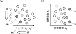
- FIG. 1A is a graph showing the relationship between two characteristic values
- FIG. 1B is a graph showing the relationship between two design variables.
- both the characteristic values f 1 and f 2 may be small.
- the two characteristic values f 1 and f 2 are preferably designed values indicated by symbols H 1 and H 2 shown in FIG.
- the design variables x 1 and x 2 have the relationship shown in FIG.
- the desired design value H 1 is a value in which the design variable x 1 and the design variable x 2 are large.
- Desirable design value H 2 is a small value is the design variables x 1, a large value is the design variables x 2.
- the design values H 1 and H 2 at which the characteristic values f 1 and f 2 are good characteristics are different from each other in the design variables x 1 and x 2 .
- the characteristic values f 1 and f 2 are good characteristics.
- the value of the design variable x 2 is an important design variable for obtaining good characteristics of the characteristic values f 1 and f 2 .
- the characteristic values f 1 and f 2 are the lateral spring constant of the tire and the rolling resistance of the tire
- the design variables x 1 and x 2 are parameters of the tire shape.
- the design variable x 2 is an important design variable for obtaining good characteristics of the characteristic values f 1 and f 2 from FIGS. 1 (a) and 1 (b). There is a case where the causal relationship is not understood.
- the present invention has been made to eliminate the difficulty in understanding such causal relationships.
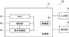
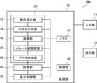
- FIG. 2 is a schematic diagram showing an example of a data processing apparatus used in the data analysis method and data display method according to the embodiment of the present invention.
- the data processing method 10 shown in FIG. 2 is used for the data analysis method and the data display method of the present embodiment.
- the data analysis method and the data display method are executed using hardware and software such as a computer. If it can do, it is not limited to the data processing apparatus 10.
- l represents the number of input data
- m represents the number of output data.
- the input value and the output value have a predetermined relationship. This predetermined relationship is a causal relationship, and means that, for example, an input value and an output value are represented by a function.
- input data representing an input value is first data representing a plurality of design variables among structures and materials constituting the structure
- output data representing an output value is the structure and structure.
- the second data representing a plurality of characteristic values.
- l is the number of design variables
- m is Represents the number of characteristic values.
- the characteristic value space corresponds to the output value space.
- the number of sets is referred to as the number of data. For example, if the number of data is 100, there are 100 sets composed of 10 data. Note that the number of input data and output data is not limited to ten as long as it is plural.
- output data are tire characteristic values, lateral spring constants, and rolling resistance
- input data are the tire shape and the components of the tire. It is a physical property value such as an elastic modulus.
- output data are the wing characteristic values, lift and mass
- input data are the shape of the wing, the elastic modulus of the members constituting the wing, etc. It is a physical property value.
- the input data (design variable) representing the input value and the output data (characteristic value) representing the output value are not particularly limited, and are calculated by a computer such as simulation or optimization. May be measured data of various tests, or may include a Pareto solution.
- the data processing device 10 includes a processing unit 12, an input unit 14, and a display unit 16.
- the processing unit 12 includes an analysis unit 20, a display control unit 22, a memory 24, and a control unit 26. In addition, although not shown, it has a ROM and the like.
- the processing unit 12 is controlled by the control unit 26.
- the analysis unit 20 is connected to the memory 24, and data of the analysis unit 20 is stored in the memory 24.
- the memory 24 stores the above-described data set input from the outside.
- the input unit 14 is various input devices for inputting various information such as a mouse and a keyboard in accordance with an operator instruction.
- the display unit 16 displays, for example, a graph using a data set, a result obtained by the analysis unit 20, and the like, and various known displays are used.
- the display unit 16 also includes a device such as a printer for displaying various types of information on an output medium.
- the data processing device 10 functionally forms each unit of the analysis unit 20 by executing a program (computer software) stored in a ROM or the like by the control unit 26.
- the data processing apparatus 10 may be configured by a computer in which each part functions by executing a program, or may be a dedicated apparatus in which each part is configured by a dedicated circuit.
- the analysis unit 20 calculates at least one of the first index and the second index in the objective function space by using a plurality of output values (characteristic values) as objective functions for the above-described data set.
- the analysis unit 20 also creates a self-organizing map using two types of data, input data and output data.
- a threshold is set for at least one of the first index and the second index, an area corresponding to the threshold on the self-organizing map is obtained, and position information on the self-organizing map is obtained.
- the analysis unit 20 creates image data so as to mark a region corresponding to the threshold value.
- the analysis unit 20 performs regression analysis using a region corresponding to the threshold on the self-organizing map. Clustering processing is performed using a region corresponding to the threshold on the self-organizing map. By this clustering process, it is determined whether the region is divided into clusters. As a result of the determination, if it is divided into clusters, a line is created using regression analysis for a cluster having a large number of regions.
- the result obtained by the analysis unit 20 is stored in the memory 24, for example.
- the display control unit 22 causes the display unit 16 to display a result obtained by analysis by the analysis unit 20, for example, a self-organizing map.
- the Pareto solution is read from the memory 24 and displayed on the display unit 16.
- the Pareto solution can be displayed in the form of a scatter diagram with the characteristic value as an axis. That is, the design variable is displayed in the characteristic value space. In addition to the scatter diagram, it can be displayed in the form of a radar chart.
- the display control unit 22 changes at least one of the color, type, and size of the symbol representing the value of the design variable according to the value of the design variable for the obtained Pareto solution.
- the obtained Pareto solution is displayed on the display unit 16 while the display form is changed by the display control unit 22. Further, the display control unit 22 has a function of displaying a line connecting the Pareto solutions for each design variable value.
- the self-organizing map also has a function of displaying each characteristic value and each design variable value.
- FIG. 3A is a graph for explaining the first index
- FIG. 3B is a graph for explaining the second index
- FIG. 3A shows a Pareto solution of the characteristic values f 1 and f 2 .
- Reference E indicates a Pareto front.
- the characteristic value has a preferable direction depending on the required specifications and the like.
- the characteristic value increases, decreases, or approaches a predetermined value.
- the first index A is represented by a distance with respect to a preset value of at least two characteristic values (objective functions) among a plurality of characteristic values (objective functions).
- the values of the characteristic values f 1 and f 2 are expressed as distances with respect to preset values.
- the first index A is the distance to the Pareto solutions E 1 from the Pareto front E.
- the first index A is not limited to the distance from the Pareto front E.
- values for at least two objective functions, in this case, characteristic values f 1 and f 2 may be set in advance, and the distance to the set values may be used as the first index A.
- the second index B is a ratio of at least two objective function values among a plurality of objective function values, in this case, a ratio of characteristic values f 1 and f 2. It is represented by Second index B is a distance B 1 between the Pareto solutions E 2 and extreme Pareto solution Ea, represented by the ratio of the Pareto solutions E 2 and extreme Pareto solutions B 2. Further, the distance may be calculated along the Pareto front E, and this may be used as the second index B.
- the second index B obtained by calculating the distance along the Pareto front E will be described with reference to FIGS. 3C and 3D, the same components as those in FIGS. 3A and 3B are denoted by the same reference numerals, and detailed description thereof is omitted.
- the Pareto front E capable linear approximation, it is possible to calculate the second index B using the distance from the approximate line L 1 .
- the Pareto front E by linear approximation to determine the approximate straight line L 1.
- a perpendicular line L 2 orthogonal to the approximate straight line L 1 is obtained. Changes sign as the center axis perpendicular L 2.
- obtaining the intersection Ph approximate lines L 1 and the perpendicular L 2. Assume that the intersection point Ph is a reference point, that is, zero, the limit Pareto solution Ea side of the intersection Ph is minus, and the limit Pareto solution Eb side of the intersection Ph is plus.
- the second index B for the point P 2 when determining the second index B for the point P 2, through the point P 2, and obtains the perpendicular line Lv perpendicular to the approximate line L 1. Then, an intersection point E 4 between the perpendicular line Lv and the approximate straight line L 1 is obtained. Next, a distance R 4 between the intersection Ph and the intersection E 4 is obtained. Since the intersection point E 4 is on the extreme Pareto solution Eb side of the intersection point Ph, a plus sign is attached. The distance R 4 is the second indicator B.
- the position of the vertical line L 2, if the approximation line L 1, is not particularly limited. Moreover, the point of obtaining a second indicator B, may be on the perpendicular L 2.
- the analysis unit 20 can create self-organizing maps shown in FIGS. Thereby, the causal relationship between the characteristic value and the design variable can be shown.
- the self-organizing map can be created using, for example, the method described in Japanese Patent No. 4339808. Therefore, detailed description of the creation of the self-organizing map is omitted.
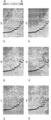
- the self-organizing maps shown in FIGS. 4A to 4H are obtained by creating self-organizing maps for the characteristic values F1 and F2 among the data sets of the characteristic values F1 to F4 and the design variables x1 to x6. It is. 4A is a self-organizing map of the characteristic value F1, and FIG. 4B is a self-organizing map of the characteristic value F2.
- FIG. 4C is a self-organizing map of the design variable x1
- FIG. 4D is a self-organizing map of the design variable x2
- FIG. 4E is a self-organizing map of the design variable x3.
- 4F is a self-organizing map of the design variable x4
- FIG. 4G is a self-organizing map of the design variable x5
- FIG. 4H is a self-organizing map of the design variable x6.
- the characteristic values F1 and F2 are, for example, lateral spring constants and rolling resistance
- the design variables x1 to x6 are parameters relating to the shape of the tire, for example.
- FIG. 5 is a flowchart showing a drawing method on the self-organizing map in the order of steps.
- the above-described data set is prepared, and the prepared data set is directly input to the analysis unit 20 via the input unit 14 or stored in the memory 24 via the input unit 14.
- the analysis unit 20 calculates the first index A or the second index B from the data set (step S10).
- the analysis unit 20 creates a self-organizing map using the data set (step S12). Thereby, for example, as described above, the self-organizing maps shown in FIGS. 4A to 4H are obtained.
- the analysis unit 20 sets a threshold value using at least one of the first index A and the second index B (step S14).
- the threshold is preferably set to 1/5 to 1/7 of the maximum value of the first index A.
- the threshold value is preferably an intermediate value.
- the analysis unit 20 obtains a region corresponding to the threshold on the self-organizing map. And the positional information on the area
- the display control unit 22 causes the display unit 16 to display a region corresponding to the threshold value together with the self-organizing map (step S16).
- the mark on the self-organizing map is not particularly limited. For example, the cell color of the self-organizing map is changed, the cell size is changed, or the cell shape is changed. And the like.
- FIG. 6A is a schematic diagram showing an example of a drawing method on the self-organizing map
- FIG. 6B is a schematic diagram showing another example of the drawing method on the self-organizing map.
- FIG. 6A shows a part of the self-organizing map, and a plurality of cells 50 constituting the self-organizing map are arranged.
- the numerical value described in the cell 50 indicates the value of the cell 50.
- the analysis unit 20 scans in the horizontal direction V and examines the numerical value of the cell 50. If the numerical value of the cell 50 is changed from 10 to 9, the numerical value before the numerical value is changed.
- the cell 52 is set as an area corresponding to the threshold value. Then, the position information of the cell 52 is stored in the memory 24, for example. In this way, in the example shown in FIG. 6A, three cells 52 are obtained as regions corresponding to the threshold values.
- the analysis unit 20 scans in the horizontal direction V. Then, when the numerical value of the cell 50 is examined and the numerical value of the cell 50 is changed from 10 to 9, the area 54 corresponding to the threshold value between the cell 50 having the numerical value 10 and the cell 50 having the numerical value 9 To do. And the positional information on the area
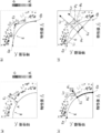
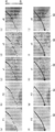
- FIG. 7A shows the first index drawn on the self-organizing map of the characteristic value F1
- FIG. 7B shows the first index drawn on the self-organizing map of the characteristic value F2.
- FIG. 7C shows the first index drawn on the self-organizing map of the first index
- FIG. 7D shows the first index drawn on the self-organizing map of the second index. It has been done.
- FIG. 8A shows the first index drawn on the self-organizing map of the design variable x1
- FIG. 8B shows the first index drawn on the self-organizing map of the design variable x2.
- FIG. 8C shows the first index drawn on the self-organizing map of the design variable x3
- FIG. 8D shows the first index on the self-organizing map of the design variable x4.
- FIG. 8E shows the first index drawn on the self-organizing map of the design variable x5
- FIG. 8F shows the self-organizing map of the design variable x6. The first index is drawn.
- the value of the self-organizing map changes along the first index. It can be seen that the ratio between the characteristic value F1 and the characteristic value F2 can be changed by changing the value of the design variable x5.
- the characteristic value F1 and the characteristic value F2 can be changed simultaneously by changing the value of the design variable x6. From this, it can be understood that the design variable x6 is an important parameter for making the characteristic values F1 and F2 compatible.
- the design variable x1 in FIG. 8A the value does not substantially change with respect to the first index.
- the design variable x1 is not an important parameter for the characteristic values F1 and F2 because the characteristic values F1 and F2 are not changed even if the value is changed.
- the causal relationship between the characteristic value and the design variable can be easily understood. Even an inexperienced analyst can easily understand.
- the second index B can be displayed on the self-organizing map in the same manner as the first index A (see FIGS. 10A to 10J).
- the image is displayed on the self-organizing map, but the present invention is not limited to this.
- the position of the region corresponding to the threshold is obtained as a result of analysis by the analysis unit 20. It may be configured to output information to the outside. Thereby, for example, using a device other than the data processing device 10, the self-organizing map on which the first index or the second index is displayed can be viewed.
- the display method is particularly limited. Is not to be done.
- a line 60 in which an arrow is attached to an end of a mark representing the first index may be used.
- the analysis unit 20 connects the areas corresponding to the threshold values to form lines.
- the method for obtaining the line 60 is not particularly limited, and a regression line may be calculated from an area corresponding to the threshold using regression analysis, and arrows may be provided at both ends of the regression line.
- the arrow of the line 60 indicates the direction in which the characteristic values F1 and F2 are compatible.
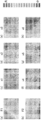
- FIGS. 10A and 10B are self-organizing maps of characteristic values in which the second index is drawn
- FIGS. 10C to 10E are design variables in which the second index is drawn.
- (F) is a self-organizing map of characteristic values in which the second index is drawn in the shape of an arrow
- (h) to (j) are the second index It is a self-organizing map of design variables drawn in the shape of arrows.
- the second index B is displayed on the self-organizing map (see FIGS. 10A to 10E) of the characteristic values F1 and F2 and the design variables x1, x5, and x6.
- FIG. ) To (j) may be a line 62 with an arrow at the end of the mark representing the second index.
- the analysis unit 20 may connect the regions corresponding to the threshold values to form lines, and provide an arrow at one end of the line 62.
- the method of obtaining the line 62 is not specifically limited, It can obtain using regression analysis similarly to the above-mentioned line 60.
- the arrow to the line 62 is attached to the end of the line 62 where the first index A is smaller.
- the arrow of the line 62 indicates the direction in which the characteristic values F1 and F2 are compatible. Also in the second index, by displaying the area corresponding to the threshold value with the line 62 instead of the point, it becomes easier to understand the causal relationship between the characteristic value and the design variable.
- the direction in which the value is smaller is determined. Specifically, in the self-organization map of the first index A shown in FIG. 7C, the end point N 1 and the end point N 2 are obtained, and the value of the cell at the end point N 1 and the value of the cell at the end point N 2 are Compare. Of endpoint N 1 and the end point N 2, defines a smaller value of the cell. Then, on the line 62 of the design variable self-organization map, an arrow is attached to the side corresponding to the end point having the smaller end point value of the first index A.
- an arrow can be attached to the line 62.
- the end point of the first index A corresponding to the second index B is obtained, and an arrow is attached to the side corresponding to the end point of the smaller cell value on the line 62 from the magnitude of the cell value of the end point.
- the analysis unit 20 can automatically calculate the above.
- the value of the design variable x6 changes along the mark.
- the values of the characteristic values F1 and F2 can be changed. From this, it can be understood that the design variable x6 is an important parameter.
- the value of the design variable x1 is not substantially changed along the mark. From this, it can be understood that the design variable x1 is a parameter that does not contribute to changing the values of the characteristic values F1 and F2.
- the value of the design variable x5 is not substantially changed along the mark. From this, it can also be understood that the contribution of the design variable x5 to the characteristic values F1 and F2 differs between the first index A and the second index B.
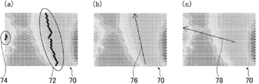
- FIG. 11A is a schematic diagram illustrating an example of the self-organizing map before the clustering process
- FIG. 11B is a schematic diagram illustrating an example of the self-organizing map subjected to the clustering process.
- c) is a schematic diagram showing an example of a self-organizing map that is not subjected to clustering processing.
- the analysis unit 20 when there are two areas corresponding to the threshold value of the first index, the first area 72 and the second area 74, the analysis unit 20 performs clustering processing. By performing regression analysis, a line 76 shown in FIG. 11B is obtained. On the other hand, when the clustering process is not performed, a line 78 shown in FIG. 11C is obtained.
- a single connection method for example, a single connection method, a complete connection method, a k-means method, or other clustering methods can be used.
- FIG. 12A shows an example of the clustering process of the self-organizing map
- FIG. 12B shows another example of the clustering process of the self-organizing map.
- the self-organizing map 70 shown in FIG. 11A there are a first region 72 and a second region 74.
- the result shown in FIG. 11B is obtained.
- the analysis unit 20 for example, with respect to the width K of the self-organizing map 70, for example, when K / 5 is a threshold and the distance is K / 5 or more, another cluster is set.
- the first area 72 and the second area 74 are determined as separate clusters.
- a regression analysis is performed on the first region 72 having a large number of regions to create a line.
- a line 76 shown in FIG. 11B can be obtained.
- the clustering process when the threshold for determining the cluster is large, it is determined that the first area 72 and the second area 74 are the same cluster, and the clustering process result shown in FIG. 12B is obtained. . Thereby, as a result of the regression analysis, for example, a line 78 shown in FIG. 11C is obtained.
- the analysis unit 20 can perform proper cluster classification, and help the analyst understand the self-organizing map. Appropriate lines can be drawn.
- FIG. 13 is a schematic diagram showing another example of a data processing apparatus used in the data analysis method and data display method according to the embodiment of the present invention.
- a data processing device 10a shown in FIG. 13 has a data processing unit 30 and is different from the data processing device 10 shown in FIG. 1 in that the above-described data set is created. Since the configuration is the same as that of the data processing apparatus 10 shown in FIG. In the data processing device 10 a shown in FIG. 13, the data processing unit 30 is connected to the analysis unit 20.
- the memory 24 and the control unit 26 are connected to the data processing unit 30, and the data processing unit 30 is controlled by the control unit 26.
- the data processing unit 30 includes a condition setting unit 32, a model generation unit 34, a calculation unit 36, a Pareto solution search unit 38, and a data creation unit 40.
- the data processing unit 30 sets two types of data, input data representing an input value and output data representing an output value, and creates a data set having a plurality of such sets.
- the data set may be directly input to the analysis unit 20 via the input unit 14 as described above without being created by the data processing unit 30. Further, the data set may be stored in the memory 24 via the input unit 14. In either case, the data processing unit 30 performs processing without creating a data set. For this reason, it is not always necessary to create a data set by the data processing unit 30.
- the condition setting unit 32 receives and sets various conditions and information necessary for displaying the Pareto solution as a scatter diagram or a self-organizing map in the characteristic value space (objective function space). Various conditions and information are input via the input unit 14. Various conditions and information set by the condition setting unit 32 are stored in the memory 24.
- condition setting unit 32 data of a data set is set, and for example, a plurality of parameters determined as design variables are set among parameters defining the structure and the material constituting the structure. In addition, you may set variation factors, such as a load and a boundary condition, in a design variable.
- data of the data set for example, a plurality of parameters defined as characteristic values (objective functions) among parameters defining the structure and the material constituting the structure are set.
- characteristic value an index for evaluating the structure and the material constituting the structure other than physical and chemical characteristic values such as cost may be used.
- the structure and the material constituting the structure may be the whole system including the structure such as the parts constituting the structure, the assembly form of the structure, or a part thereof, instead of the structure alone.
- the characteristic value set in the condition setting unit 32 is a physical quantity to be evaluated.
- the objective function is a function for obtaining a physical quantity to be evaluated.
- the characteristic value is a characteristic value of the tire.
- the characteristic value is a physical quantity to be evaluated as tire performance, for example, a CP (cornering power) which is a lateral force at a slip angle of 1 degree, which is an indicator of steering stability, and an indicator of steering stability.
- the tire's primary tread frequency as an indicator of cornering characteristics, riding comfort, rolling resistance as an indicator of rolling resistance, lateral spring constant as an indicator of steering stability, tire tread member as an indicator of wear resistance For example, wear energy.
- the objective function is a function for obtaining them.
- the objective function has a preferable direction in terms of performance, and the value increases, decreases, or approaches a predetermined value.
- the design variable defines the shape of the structure, the internal structure of the structure, the material characteristics, and the like.
- design variables are a plurality of parameters among tire material behavior, tire shape, tire cross-sectional shape, and tire structure.
- the design variable include a radius of curvature that defines a crown shape in a tread portion of the tire, a belt width dimension of the tire that defines a tire internal structure, and the like.
- a filler dispersion shape that defines material characteristics in the tread portion, a filler volume ratio, and the like can be given.
- the constraint condition is a condition for constraining the value of the objective function to a predetermined range or constraining the value of the design variable to a predetermined range.
- vehicle running simulation such as tire load load, running conditions such as tire rolling speed, road surface conditions where the tire runs, for example, uneven shape, friction coefficient, etc. Information on the vehicle specifications is set.
- condition setting unit 32 information for determining the nonlinear response relationship between the design variable and the characteristic value parameter is set in the condition setting unit 32.
- This nonlinear response relationship includes, for example, a numerical simulation such as FEM, a theoretical expression, an approximate expression, and the like.
- the condition setting unit 32 in the case of performing a numerical simulation such as a model generated by a non-linear response relationship, a boundary condition of the model, and FEM, the simulation condition and a constraint condition in the simulation are set.
- an optimization condition for obtaining a Pareto solution for example, a condition for searching for a Pareto solution is set.
- the conditions for the Pareto solution search are a method for searching for the Pareto solution and various conditions in the Pareto solution search.
- a genetic algorithm can be used as a method for searching for a Pareto solution.
- the exploration ability of a genetic algorithm decreases as the objective function increases.
- One way to solve this is to increase the number of individuals.
- Pareto solutions are searched, many Pareto solutions are calculated. Therefore, a method for displaying the causal relationship between a large amount of characteristic value data and design parameters with high visibility is one of the problems in design exploration, but the present invention can solve this.
- the condition setting unit 32 sets the definition area of the design variable. Further, the condition setting unit 32 sets discrete values used when contracting the Pareto solution, as will be described later.
- the model generation unit 34 creates various calculation models based on the set nonlinear response relationship.
- the non-linear response relationship includes a numerical simulation such as FEM.
- the model generation unit 34 generates a mesh model corresponding to a design parameter representing a design variable and a characteristic value parameter representing a characteristic value. Is done.
- theoretical formulas and approximate formulas theoretical formulas and approximate formulas corresponding to design parameters and characteristic value parameters are created.
- the calculation unit 36 performs a simulation calculation using the tire model.
- the tire model created by the model generation unit 34 is created by using each type of design parameters set by the condition setting unit 32.
- a known creation method can be used for creating the tire model.
- the tire model also generates at least a road surface model that is a target for rolling the tire model.
- a tire model that reproduces a rim on which a tire is mounted, a wheel, and a tire rotation axis may be used. Further, if necessary, a model that reproduces a vehicle to which a tire is attached may be incorporated into the tire model.
- a model in which the tire model, the rim model, the wheel model, and the tire rotation axis model are integrated based on a preset boundary condition can be created.
- These models may be discretized models capable of numerical calculation, and may be, for example, finite element models for use in a known finite element method (FEM).
- FEM finite element method
- the inclusions existing on the road surface are reproduced, for example, when a tire design plan that optimizes tire performance such as tire wet performance is obtained using the tire model.
- Generate a model For example, as an inclusion model, various models that reproduce water, snow, mud, sand, gravel, ice, or the like on a road surface may be generated as a discretized model that can be numerically calculated.
- the road surface model is not limited to a model that reproduces a road surface with a flat surface, and may be a model that reproduces a road surface shape having irregularities on the surface as necessary.
- the calculation unit 36 calculates characteristic values using various models created by the model generation unit 34. Thereby, a characteristic value for the setting variable is obtained. Among these characteristic values, there is a Pareto solution. The obtained characteristic value is stored in the memory 24.
- the calculation unit 36 for example, the behavior of the tire model when a simulation condition for reproducing the rolling of the tire rolling on the road surface is given to the tire model generated by the model generation unit 34, the road surface model, or the like, or A physical quantity such as force acting on the tire model is obtained in time series.
- the calculation unit 36 functions by executing a subroutine by a known finite element solver, for example.
- the model generation unit 34 creates a theoretical formula, an approximate formula, and the like, the theoretical formula, the approximate formula, and the like are solved, and a characteristic value is calculated.
- the Pareto solution search unit 38 searches for the Pareto solution from the characteristic values obtained by the calculation unit 36 in accordance with the Pareto solution search conditions set by the condition setting unit 32, and calculates a Pareto solution. is there.
- the obtained Pareto solution is stored in the memory 24.
- the Pareto solution is a solution in which a plurality of objective functions that are in a trade-off relationship are not superior to any other arbitrary solution, but no other superior solution exists.
- the Pareto solution search unit 38 searches for a Pareto solution using, for example, a genetic algorithm. Genetic algorithms include, for example, DRMOGA (Divided Range Multi-Objective GA), NCGA (Neighborhood Cultivation GA), which divides a solution set into a plurality of regions along an objective function and performs multi-objective GA for each divided solution set.
- DRMOGA Divided Range Multi-Objective GA
- NCGA Neighborhood Cultivation GA
- the Pareto solution search unit 38 performs selection using, for example, a vector evaluation genetic algorithm (VEGA), a Pareto ranking method, or a tournament method.
- VEGA vector evaluation genetic algorithm
- SA annealing
- PSO particle swarm optimization
- Nonlinear response relationship defined between design variable (input value) and characteristic value (output value), that is, what is used when obtaining characteristic value using design variable is limited to simulation such as FEM
- theoretical formulas and approximate formulas can be used as described above.
- the value of the objective function may be calculated using a simulation approximation formula instead of the calculation using the simulation model.
- a Pareto solution can be obtained from an experimental result obtained based on the experimental design using an approximate expression between the design variable and the objective function, for example, a simulation approximate expression.
- a known nonlinear function obtained by a polynomial or a neural network can be used.
- the data creation unit 40 reads the Pareto solution obtained by the Pareto solution search unit 38 and stored in the memory 24, and the objective function data from the memory 24, and includes two types of data representing design variables and data representing characteristic values. The data set which made the data of this is made. The data set created by the data creation unit 40 is stored in the memory 24.
- FIG. 14 is a flowchart showing an example of the data analysis method according to the embodiment of the present invention in the order of steps.
- design variables and characteristic values are set for the target structure.
- the structure is, for example, a tire.
- a tire shape parameter is set as a design variable for the tire.
- two of the rolling resistance and the lateral spring constant are set as characteristic values.
- the input is a tire shape parameter
- the output is a rolling resistance and a lateral spring constant. Displays how the rolling resistance and the lateral spring constant change depending on the value of the tire shape parameter.
- the tire shape parameters, rolling resistance and lateral spring constant are set in the condition setting unit 32.
- a nonlinear response to be used when obtaining the characteristic value from the design variable is determined (step S20). That is, the relationship between design variables and characteristic values is determined.
- the type of this nonlinear response is stored in the memory 24, for example.
- the relationship between the tire shape parameter, the rolling resistance and the lateral spring constant is set.
- the relationship to be set is expressed using a nonlinear function such as a quadratic polynomial in which the rolling resistance has the tire shape parameter as a variable.
- the lateral spring constant is expressed using a nonlinear function such as a second-order polynomial with the tire shape parameter as a variable.
- a design variable definition area is set (step S22).
- an upper limit value and a lower limit value are set for the parameters of the design variable, and the interval between the lower limit value and the upper limit value is continuous.
- the upper and lower limits of the size are set as the domain of the design variable on the assumption that the range between the lower limit value and the upper limit value is continuous.
- the upper limit and the lower limit of the elastic modulus are set as the definition area of the design variable.
- the definition area of the design variable is set by the condition setting unit 32 and stored in the memory 24, for example.
- an upper limit value and a lower limit value are set for the tire shape parameters.
- the model generation unit 34 creates a model based on the nonlinear response relationship
- the calculation unit 36 calculates a characteristic value based on the nonlinear response relationship set in step S20 (step S24).
- the definition area of the set design variable is read from the memory 24 and the characteristic value is calculated.
- the calculation result of the characteristic value is stored in the memory 24, for example.
- a simulation such as FEM
- a mesh model is created by the model generation unit 34, and a response to an input is simulated by the calculation unit 36 by FEM or the like. Specifically, the rolling resistance and the lateral spring constant for the tire shape parameter are calculated.
- the Pareto solution search unit 38 performs optimization using the characteristic value as an objective function for the calculation result of the characteristic value, thereby obtaining a Pareto solution (step S26). For example, a genetic algorithm is used to calculate the Pareto solution.
- the obtained Pareto solution is stored in the memory 24.
- the data processing apparatus 10a calculates the Pareto solution, and then the data creation unit 40 creates a data set.
- the analysis unit 20 performs various data processing using the created data set. Thereafter, as necessary, the self-organizing map can be displayed on the display unit 16 via the display control unit 22 as necessary.
- the data processing device 10a can display a region based on the first index or the second index on the self-organization map in the same manner as the data processing device 10 described above except that a Pareto solution is created. Detailed description thereof will be omitted. Even in this case, even an inexperienced analyst can easily understand the causal relationship between input values and output values, important design variables (input values), and the like. In addition, information that can be easily understood can be obtained.
- FIG. 15 is a schematic diagram showing another example of a data processing apparatus used in the data analysis method and data display method according to the embodiment of the present invention.
- the data processing device 10b shown in FIG. 15 has a moving average processing unit 28, and is different from the data processing device 10 shown in FIG. 1 in that the moving average processing is performed on the above-described data set. Since the configuration is the same as that of the data processing apparatus 10 shown in FIG. 1, detailed description thereof is omitted.
- FIG. 16 is a flowchart showing the moving average process of the data analysis method according to the embodiment of the present invention in the order of steps.
- the average section is a setting area for obtaining an average value of master points, which will be described later, when performing moving average processing.
- This average area is appropriately set according to the data type of the input data of the data set, for example, the number of input parameters and the data type of the output data, for example, the number of output parameters, and the shape and the like are particularly limited. It is not something.
- the average interval is, for example, a polygon such as a rectangle, a circle, or the like The two-dimensional shape.
- the average interval is, for example, a polygonal column such as a quadrangular prism, and a sphere or the like 3 Dimensional shape.
- the average interval is, for example, a hypercube, a hypersphere, or the like.
- the size of the average section is not particularly limited.
- the output value space may be normalized when setting the average interval. That is, a characteristic value space described later may be normalized.
- the function w (r) of the following equation (1) can be used as the weighting function for the average interval.
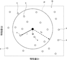
- the function w (r) of the following formula (1) is as shown in FIG.
- r 0 represents the size of the average interval
- r represents the distance between the master point and the slave point.
- r 0 is the radius of a circle if the average interval is a circle, and the radius of a hypersphere if it is a hypersphere.
- the distance r 1.0 between the master point and the slave point is the size of the average section.
- the weighting function is not limited to the function of the above formula (1), and may be a constant value within the average interval as indicated by a symbol C in FIG.
- the constant value is not particularly limited, but is 1.0 in the example shown in FIG.
- at least one of the average interval and the weight function may be changed according to the density of the data in the output value space.
- a master point is set from input data composed of design variables (step S32).
- a slave point is set from input data composed of design variables (step S34).
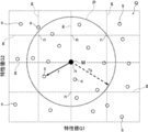
- the master point is selected from the existing input data within the average interval P.
- Set M the points other than the master point M become slave points s.
- Data at the master point M is master data
- data at the slave point s is slave data.
- a setting method of the master point M for example, as shown in FIG.
- a grid g may be set in the characteristic value space Q, and the intersection point n of the grid g may be set as the master point M.
- the master point M is not necessarily input data that exists.
- the size of the grid g is not particularly limited, and is appropriately set according to the number of data.
- step S36 the distance r between the master point and the slave point on the characteristic value space Q is calculated (step S36).
- a known distance calculation method between two coordinates can be used.
- step S36 if the calculated distance is within the average period P, that, if a r ⁇ r 0, to calculate the value of the weight (w v) using a weighting function, the value of the weight (w v) Is stored in the memory 24, for example.
- a value (w v x) of the product of the input data value and the weight value is calculated by multiplying the value of each input data of the input value, for example, the value (x) of the design variable by the weight value.
- the product value (w v x) of the calculated input data value and weight value is stored in, for example, the memory 24 (step S38).
- the value (w v x) of the product of the input data value and the weight value is calculated for each input data. That is, for each design variable, the product value (w v x) of the design variable value (x) and the weight value is calculated.
- the sum of one sum (w Vtot) and the input data value and the product of the value of the weight values of the weight values of the master points M (w v) (w v x) (w v x tot) Is obtained for each design variable.
- step S42 it is determined whether or not calculation processing is performed on all the sets of data sets excluding data of the data set as master points as slave points.
- the calculation process in step S42 can be determined by comparing the number of data in the data set with the calculated number of slave data.
- step S42 when the data of the data set excluding the data as the master point is calculated as the slave point, the value (w v x) of the product of the input data value and the weight value is calculated for each input data.
- step S44 the average value of the design variables around the master point M can be obtained for each design variable in the average interval P shown in FIGS.
- Step S34 slave point setting
- step S40 weight / design variable product calculation
- step S46 it is determined whether or not all the sets of data sets have been calculated as master points M (step S46).
- step S46 the moving average process ends when all the sets of data sets have been calculated as the master point M.
- the calculation process in step S42 can be determined.
- the master point M is the intersection point n of the grid g
- the calculation process in step S42 can be determined by comparing the number of intersection points n with the calculated number of master points M.
- step S46 in the case where calculation processing is not performed on all the sets of data sets as master points M, in order to set all the sets of data sets as master points M, the above-described step S32 (setting of master points) is performed. To step S44 (calculation of the average value of the master points) is repeated. In step S46, when the calculation process is performed on all the sets of data sets as the master point M, the moving average process ends. As described above, the moving average process of input data in the output value space, for example, the moving average process of design variables in the characteristic value space is completed.
- the analysis unit 20 performs various data processing.
- the self-organizing map can be displayed on the display unit 16 via the display control unit 22 as necessary.
- the data processing device 10b displays an area based on the first index or the second index on the self-organizing map in the same manner as the data processing device 10 described above except that the moving average processing is performed on the data set. Therefore, detailed description thereof is omitted.
- the moving average process when a region corresponding to the threshold value is displayed on the self-organizing map, the causal relationship between the output value and the input data can be found more easily. Even in this case, even an inexperienced analyst can easily understand the causal relationship between input values and output values, important design variables (input values), and the like. In addition, information that can be easily understood can be obtained.
- the moving average processing unit 28 performs the moving average processing on the data set prepared in advance, but the present invention is not limited to this.
- a data processing unit 30 is provided, a Pareto solution is calculated by the data processing unit 30, and a moving average process is performed by the moving average processing unit 28 on a data set including the calculated Pareto solution.
- the structure which gives may be sufficient.
- the data processing unit 30 has the same configuration as that of the data processing device 10a in FIG. 13, and thus detailed description thereof is omitted.
- the data processing device 10c also displays an area based on the first index or the second index on the self-organizing map in the same manner as the data processing device 10, except that a Pareto solution is created and a moving average process is performed. Therefore, detailed description thereof is omitted. Even in this case, even an inexperienced analyst can easily understand the causal relationship between input values and output values, important design variables (input values), and the like. In addition, information that can be easily understood can be obtained.
- the present invention is basically configured as described above.
- the data analysis method and data display method of the present invention have been described in detail above.
- the present invention is not limited to the above-described embodiment, and various improvements or modifications can be made without departing from the spirit of the present invention. Of course it is also good.
Landscapes
- Engineering & Computer Science (AREA)
- Theoretical Computer Science (AREA)
- Physics & Mathematics (AREA)
- General Engineering & Computer Science (AREA)
- General Physics & Mathematics (AREA)
- Evolutionary Computation (AREA)
- Computer Hardware Design (AREA)
- Geometry (AREA)
- Software Systems (AREA)
- Mathematical Physics (AREA)
- Computing Systems (AREA)
- Biophysics (AREA)
- Life Sciences & Earth Sciences (AREA)
- Artificial Intelligence (AREA)
- Biomedical Technology (AREA)
- Health & Medical Sciences (AREA)
- Computational Linguistics (AREA)
- Data Mining & Analysis (AREA)
- General Health & Medical Sciences (AREA)
- Molecular Biology (AREA)
- Information Retrieval, Db Structures And Fs Structures Therefor (AREA)
- User Interface Of Digital Computer (AREA)
Abstract
データの分析方法は、所定の関係を有する複数の入力値と複数の出力値において、複数の入力値を表わす入力データと、複数の出力値を表わす出力データの2種類のデータを対象としている。複数の出力値を目的関数として、目的関数空間における第1の指標および第2の指標の少なくとも一方を求める工程を有する。第1の指標は複数の目的関数の値のうち、少なくとも2つの目的関数の値の、予め設定された値に対する距離である。第2の指標は複数の目的関数の値のうち、少なくとも2つの目的関数の値の比率で表されるものである。
Description
本発明は、所定の関係を有する複数の入力値と複数の出力値において、複数の入力値を表わす入力データと、複数の出力値を表わす出力データの2種類のデータを対象として、コンピュータ等を用いたデータの分析方法およびデータの表示方法に関し、特に、複数の入力値と、複数の出力値との因果関係の理解を容易にするためのデータの分析方法およびデータの表示方法に関する。
構造体および構造体を構成する材料の設計変数を入力値とし、構造体および構造体を構成する材料のうち複数の特性値(目的関数)を出力値として、多目的最適化とデータマイニングを組合せて用いることで、設計変数と特性値との因果関係を見出すことができることが知られている。
複数の特性値(目的関数)を対象とする多目的最適化では、特性値の間にトレードオフ関係が存在することが少なくない。その場合、最適解はパレート解と呼ばれる解集合を形成する。そのパレート解と設計変数との因果関係を分析することで特定の特性値バランスを実現するための設計変数の方向性を知ることができ、その情報を設計に役立てることができる。パレート解のデータから、特性値と設計変数の因果関係を分析する従来の方法として、自己組織化マップが提案されている(非特許文献1参照)。
複数の特性値(目的関数)を対象とする多目的最適化では、特性値の間にトレードオフ関係が存在することが少なくない。その場合、最適解はパレート解と呼ばれる解集合を形成する。そのパレート解と設計変数との因果関係を分析することで特定の特性値バランスを実現するための設計変数の方向性を知ることができ、その情報を設計に役立てることができる。パレート解のデータから、特性値と設計変数の因果関係を分析する従来の方法として、自己組織化マップが提案されている(非特許文献1参照)。
非特許文献1では、自己組織化マップを用い、この自己組織化マップ上に目的関数、設計変数を表示することができ、それらを並べて表示することで、視覚的に目的関数間の相関関係を把握できるだけでなく、目的関数と設計変数との因果関係も理解できることが記載されている。
日本ゴム協会誌、Vol.85、2012、289-295.
上述のように、非特許文献1に自己組織化マップを用いて特性値(出力値)と設計変数(入力値)の因果関係を分析することが記載されている。
ここで、多目的最適化問題において複数の特性値を向上させる設計値を探索することが重要である。同時に設計変数空間において、複数の特性値を向上させる設計変数が何かを判別することも重要である。しかしながら、通常の製品設計では設計変数、特性値の数はきわめて多く、どの設計変数の寄与が大きいか判別しづらい。また経験の浅い解析者では結果を図示しても因果関係が理解できないことがあるという問題点がある。
また、特性値と設計変数の因果関係を可視化した自己組織化マップでは、解析者が理解し易いようにデータをまとめてはいるが、経験の浅い解析者では、どの因子が特性値に影響を与えているか理解しにくいという問題点がある。
ここで、多目的最適化問題において複数の特性値を向上させる設計値を探索することが重要である。同時に設計変数空間において、複数の特性値を向上させる設計変数が何かを判別することも重要である。しかしながら、通常の製品設計では設計変数、特性値の数はきわめて多く、どの設計変数の寄与が大きいか判別しづらい。また経験の浅い解析者では結果を図示しても因果関係が理解できないことがあるという問題点がある。
また、特性値と設計変数の因果関係を可視化した自己組織化マップでは、解析者が理解し易いようにデータをまとめてはいるが、経験の浅い解析者では、どの因子が特性値に影響を与えているか理解しにくいという問題点がある。
本発明の目的は、前述の従来技術に基づく問題点を解消し、入力値(設計変数)が複数あり、出力値(特性値)が複数ある場合において、入力値(設計変数)と出力値(特性値)との因果関係の理解を容易にするデータの分析方法およびデータの表示方法を提供することにある。
上記目的を達成するために、本発明は、所定の関係を有する複数の入力値と複数の出力値において、前記複数の入力値を表わす入力データと、前記複数の出力値を表わす出力データの2種類のデータを対象としたデータの分析方法であって、前記複数の出力値を目的関数として、目的関数空間における第1の指標および第2の指標の少なくとも一方を求める工程を有し、前記第1の指標は、複数の目的関数の値のうち、少なくとも2つの目的関数の値の、予め設定された値に対する距離であり、前記第2の指標は、複数の目的関数の値のうち、少なくとも2つの目的関数の値の比率で表されるものであることを特徴とするデータの分析方法を提供するものである。
さらに、前記入力データおよび前記出力データの前記2種類のデータを用いて、自己組織化マップを作成する工程と、前記第1の指標および前記第2の指標のうち、少なくとも一方を用いて閾値を設定する工程と、前記自己組織化マップ上での前記閾値に対応する領域を求める工程とを有することが好ましい。
さらに、前記自己組織化マップ上で前記閾値に対応する前記領域を用いて回帰分析をする工程とを有することが好ましい。
さらに、前記自己組織化マップ上で前記閾値に対応する前記領域を用いて回帰分析をする工程とを有することが好ましい。
さらに、前記自己組織化マップ上で前記閾値に対応する前記領域を用いてクラスタリング処理をする工程と、前記クラスタリング処理により、前記領域がクラスタに分けられるかを判定する工程と、前記クラスタに分けられる場合、前記領域の数が多いクラスタについて回帰分析を用いて線を作成する工程とを有することが好ましい。
例えば、前記入力値を表わす前記入力データは、構造体および構造体を構成する材料の設計変数を表すものであり、前記出力値を表わす前記出力データは、構造体および構造体を構成する材料の特性値を表すものである。例えば、前記出力データは、パレート解を含む。
例えば、前記入力値を表わす前記入力データは、構造体および構造体を構成する材料の設計変数を表すものであり、前記出力値を表わす前記出力データは、構造体および構造体を構成する材料の特性値を表すものである。例えば、前記出力データは、パレート解を含む。
また、本発明は、所定の関係を有する複数の入力値と複数の出力値において、前記複数の入力値を表わす入力データと、前記複数の出力値を表わす出力データの2種類のデータを対象としたデータの表示方法であって、前記複数の出力値を目的関数として、目的関数空間における第1の指標および第2の指標の少なくとも一方を求める工程と、前記第1の指標および前記第2の指標の少なくとも一方を、前記入力データおよび前記出力データの前記2種類のデータと共に、表示する工程と、前記入力データおよび前記出力データの前記2種類のデータを用いて、自己組織化マップを作成する工程と、前記第1の指標および前記第2の指標のうち、少なくとも一方を用いて閾値を設定する工程と、前記自己組織化マップ上での前記閾値に対応する領域を求める工程と、前記自己組織化マップ上で前記閾値に対応する前記領域に印をつけて表示する工程とを有し、前記第1の指標は、複数の目的関数の値のうち、少なくとも2つの目的関数の値の、予め設定された値に対する距離であり、前記第2の指標は、複数の目的関数の値のうち、少なくとも2つの目的関数の値の比率で表されるものであることを特徴とするデータの表示方法を提供するものである。
さらに、前記入力データおよび前記出力データの前記2種類のデータを用いて、自己組織化マップを作成する工程と、前記第1の指標および前記第2の指標のうち、少なくとも一方を用いて閾値を設定する工程と、前記自己組織化マップ上での前記閾値に対応する領域を求める工程と、前記自己組織化マップ上で前記閾値に対応する前記領域に印をつけて表示する工程とを有することが好ましい。
さらに、前記自己組織化マップ上で前記閾値に対応する前記領域を用いて回帰分析をする工程と、前記回帰分析の結果を前記自己組織化マップ上に表示する工程とを有することが好ましい。
さらに、前記自己組織化マップ上で前記閾値に対応する前記領域を用いて回帰分析をする工程と、前記回帰分析の結果を前記自己組織化マップ上に表示する工程とを有することが好ましい。
さらに、前記自己組織化マップ上で前記閾値に対応する前記領域を用いてクラスタリング処理をする工程と、前記クラスタリング処理により、前記領域がクラスタに分けられるかを判定する工程と、前記クラスタに分けられる場合、前記領域の数が多いクラスタについて回帰分析を用いて線を作成し、前記クラスタの近似式で表される前記線を、前記自己組織化マップ上に表示する工程とを有することが好ましい。
例えば、前記入力値を表わす前記入力データは、構造体および構造体を構成する材料の設計変数を表すものであり、前記出力値を表わす前記出力データは、構造体および構造体を構成する材料の特性値を表すものである。例えば、前記出力データは、パレート解を含む。
例えば、前記入力値を表わす前記入力データは、構造体および構造体を構成する材料の設計変数を表すものであり、前記出力値を表わす前記出力データは、構造体および構造体を構成する材料の特性値を表すものである。例えば、前記出力データは、パレート解を含む。
本発明のデータの分析方法によれば、入力値が複数あり、出力値が複数ある場合において、入力値と出力値との因果関係を、例えば、経験の浅い解析者であっても容易に理解できる。
また、本発明のデータの表示方法によれば、入力値が複数あり、出力値が複数ある場合において、入力値と出力値との因果関係を、例えば、経験の浅い解析者であっても視覚的に容易に理解することができる。
また、本発明のデータの表示方法によれば、入力値が複数あり、出力値が複数ある場合において、入力値と出力値との因果関係を、例えば、経験の浅い解析者であっても視覚的に容易に理解することができる。
以下に、添付の図面に示す好適実施形態に基づいて、本発明のデータの分析方法およびデータの表示方法を詳細に説明する。
図1(a)は2つの特性値の関係を示すグラフであり、(b)は2つの設計変数の関係を示すグラフである。
図1(a)は2つの特性値の関係を示すグラフであり、(b)は2つの設計変数の関係を示すグラフである。
設計変数x1、x2の関数である2つの特性値f1、f2において、図1(a)に示すように、例えば、特性値f1、f2がいずれも値が小さくなることが好ましい場合、2つの特性値f1、f2は、図1(a)に示す符号H1、H2で示す設計値が望ましい。なお、設計変数x1、x2は、図1(b)に示す関係を有する。
図1(b)に示すように、望ましい設計値H1は、設計変数x1および設計変数x2が大きい値である。望ましい設計値H2は、設計変数x1が小さい値であり、設計変数x2が大きい値である。このように、特性値f1、f2が良好な特性となる設計値H1、設計値H2は設計変数x1、x2の値が異なる。しかし、設計変数x2の値が大きいと特性値f1、f2は良好な特性となる。設計変数x2の値が特性値f1、f2の良好な特性を得るに重要な設計変数である。例えば、特性値f1、f2は、タイヤの横ばね定数、タイヤの転がり抵抗であり、設計変数x1、x2は、タイヤの形状のパラメータである。
図1(b)に示すように、望ましい設計値H1は、設計変数x1および設計変数x2が大きい値である。望ましい設計値H2は、設計変数x1が小さい値であり、設計変数x2が大きい値である。このように、特性値f1、f2が良好な特性となる設計値H1、設計値H2は設計変数x1、x2の値が異なる。しかし、設計変数x2の値が大きいと特性値f1、f2は良好な特性となる。設計変数x2の値が特性値f1、f2の良好な特性を得るに重要な設計変数である。例えば、特性値f1、f2は、タイヤの横ばね定数、タイヤの転がり抵抗であり、設計変数x1、x2は、タイヤの形状のパラメータである。
上述のように、多目的最適化問題において複数の特性値を向上させる設計値を探索することが重要である。同時に設計変数空間において、複数の特性値を向上させる設計変数が何かを判別することも重要である。しかしながら、通常の製品設計では設計変数、特性値の数はきわめて多く、どの設計変数の寄与が大きいか判別しづらい。また、経験の浅い解析者では結果を図示しても、図1(a)、(b)から設計変数x2の値が特性値f1、f2の良好な特性を得るに重要な設計変数であるという、因果関係が理解できないことがある。本発明は、このような因果関係の理解の困難さを解消するためになされたものである。
図2は本発明の実施形態のデータの分析方法およびデータの表示方法に利用されるデータ処理装置の一例を示す模式図である。
本実施形態のデータの分析方法およびデータの表示方法には、図2に示すデータ処理装置10が用いられるが、データの分析方法およびデータの表示方法をコンピュータ等のハードウェアおよびソフトウェアを用いて実行することができればデータ処理装置10に限定されるものではない。
入力値を表わす入力データXi(i=1,l)と、出力値を表わす出力データYj(j=1,m)の2種類のデータを組としたデータセットを対象としており、出力値空間において分析し、その結果を表示する。なお、lは入力データの数、mは出力データの数を表わす。入力値および特性値は、それぞれ複数ある。入力値と出力値とは所定の関係を有する。この所定の関係とは、因果関係であり、例えば、入力値と出力値とが関数により表わされることをいう。
データセットにおいて、例えば、入力値を表わす入力データは構造体および構造体を構成する材料のうち、複数の設計変数を表す第1のデータであり、出力値を表わす出力データは構造体および構造体を構成する材料のうち、複数の特性値を表す第2のデータである。この場合、第1のデータが入力データXi(i=1,l)に相当し、第2のデータが出力データYj(j=1,m)に相当し、lは設計変数の数、mは特性値の数を表す。特性値空間が出力値空間に対応する。
データセットでは、例えば、l=6、m=2のとき、入力データX1~X6と出力データY1~Y4の合計10のデータを1組として扱い、この10のデータの組(入力データX1~X6、出力データY1~Y4)が複数組存在する。データセットにおいて、上記組の数をデータ数という。例えば、データ数が100であれば、10のデータで構成される組が100存在する。なお、入力データと出力データの数は、複数であればよく、特に10に限定されるものではない。
データセットでは、例えば、l=6、m=2のとき、入力データX1~X6と出力データY1~Y4の合計10のデータを1組として扱い、この10のデータの組(入力データX1~X6、出力データY1~Y4)が複数組存在する。データセットにおいて、上記組の数をデータ数という。例えば、データ数が100であれば、10のデータで構成される組が100存在する。なお、入力データと出力データの数は、複数であればよく、特に10に限定されるものではない。
例えば、タイヤの設計に利用する場合、出力データ(特性値)は、タイヤの特性値、横ばね定数、ころがり抵抗であり、入力データ(設計変数)は、タイヤの形状、タイヤを構成する部材の弾性率等の物性値である。例えば、翼の設計に利用する場合、出力データ(特性値)は、翼の特性値、揚力、質量であり、入力データ(設計変数)は、翼の形状、翼を構成する部材の弾性率等の物性値である。
なお、データセットにおいては、入力値を表わす入力データ(設計変数)と出力値を表わす出力データ(特性値)のデータは、特に限定されるものではなく、シミュレーションまたは最適化のようなコンピュータ演算されたものでもよいし、各種試験の計測データでもよく、また、パレート解を含んでもよい。
なお、データセットにおいては、入力値を表わす入力データ(設計変数)と出力値を表わす出力データ(特性値)のデータは、特に限定されるものではなく、シミュレーションまたは最適化のようなコンピュータ演算されたものでもよいし、各種試験の計測データでもよく、また、パレート解を含んでもよい。
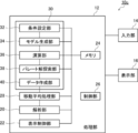
データ処理装置10は、処理部12と、入力部14と、表示部16とを有する。処理部12は、解析部20、表示制御部22、メモリ24および制御部26を有する。この他に図示はしないがROM等を有する。
処理部12は、制御部26により制御される。また、処理部12において解析部20はメモリ24に接続されており、解析部20のデータがメモリ24に記憶される。また、メモリ24には、外部から入力される上述のデータセットが記憶される。
処理部12は、制御部26により制御される。また、処理部12において解析部20はメモリ24に接続されており、解析部20のデータがメモリ24に記憶される。また、メモリ24には、外部から入力される上述のデータセットが記憶される。
入力部14は、マウスおよびキーボード等の各種情報をオペレータの指示により入力するための各種の入力デバイスである。表示部16は、例えば、データセットを用いたグラフ、解析部20で得られた結果等を表示するものであり、公知の各種のディスプレイが用いられる。また、表示部16には各種情報を出力媒体に表示するためのプリンタ等のデバイスも含まれる。
データ処理装置10は、ROM等に記憶されたプログラム(コンピュータソフトウェア)を、制御部26で実行することにより、解析部20の各部を機能的に形成する。データ処理装置10は、上述のように、プログラムが実行されることで各部位が機能するコンピュータによって構成されてもよいし、各部位が専用回路で構成された専用装置であってもよい。
解析部20は、上述のデータセットについて、複数の出力値(特性値)を目的関数として、目的関数空間における第1の指標および第2の指標のうち、少なくとも一方を算出するものである。
また、解析部20は、入力データおよび出力データの2種類のデータを用いて、自己組織化マップを作成する。第1の指標および第2の指標のうち、少なくとも一方に対して閾値を設定し、自己組織化マップ上での閾値に対応する領域を求め、その自己組織化マップ上での位置情報を得る。さらには、解析部20は、閾値に対応する領域に印をつけるように画像データを作成する。
解析部20は、自己組織化マップ上で閾値に対応する領域を用いて回帰分析をする。自己組織化マップ上で閾値に対応する領域を用いてクラスタリング処理をする。このクラスタリング処理により、領域がクラスタに分けられるかを判定する。判定の結果、クラスタに分けられる場合、領域の数が多いクラスタについて回帰分析を用いて線を作成する。
解析部20で得られた結果は、例えば、メモリ24に記憶される。
表示制御部22は、解析部20で解析して得られた結果、例えば、自己組織化マップ等を表示部16に表示させるものである。それ以外にも、パレート解をメモリ24から読み出し、表示部16に表示させる。この場合、例えば、特性値を軸にとって、パレート解を散布図の形態で表示することもできる。すなわち、特性値空間に設計変数を表示する。散布図以外にも、レーダチャートの形態で表示することができる。
また、表示制御部22は、例えば、得られたパレート解について、設計変数の値に応じて、設計変数の値を表すシンボルの色、種類および大きさのうち、少なくとも1つを変える。表示形態を変更したパレート解の情報はメモリ24に記憶される。得られたパレート解は、表示制御部22で表示形態が変えられて表示部16で表示される。さらには、表示制御部22では、設計変数の値毎に、そのパレート解を結んだ線を表示させる機能も有する。自己組織化マップについても、特性値の値毎に、設計変数の値毎に表示させる機能も有する。
次に、データ分析方法で計算する第1の指標および第2の指標について説明する。
図3(a)は第1の指標を説明するためのグラフであり、(b)は第2の指標を説明するためのグラフである。
図3(a)に特性値f1、f2のパレート解を示す。符号Eはパレートフロントを示す。特性値は、要求される仕様等に応じて好ましい方向があり、値が大きくなる、値が小さくなる、または所定の値に近づく等がある。第1の指標Aは、複数の特性値(目的関数)の値のうち、少なくとも2つの特性値(目的関数)の値の、予め設定された値に対する距離で表される。すなわち、特性値f1、f2の値に値して、予め設定された値に対する距離で表される。
例えば、第1の指標Aは、パレートフロントEからのパレート解E1迄の距離である。なお、第1の指標Aは、パレートフロントEからの距離に限定されるものではない。例えば、少なくとも2つの目的関数の値、この場合、特性値f1、f2について、予め値を設定しておき、この設定された値に対する距離を、第1の指標Aとすることもできる。
図3(b)に示すように、第2の指標Bは、複数の目的関数の値のうち、少なくとも2つの目的関数の値の比率、この場合、特性値f1、f2の値の比率で表されるものである。第2の指標Bは、パレート解E2と極限パレート解Eaとの距離B1と、パレート解E2と極限パレート解B2との比率で表される。
また、パレートフロントEに沿って距離を算出し、これを第2の指標Bとしてもよい。以下、図3(c)、(d)を用いて、パレートフロントEに沿って距離を算出して得る第2の指標Bについて説明する。なお、図3(c)、(d)において、図3(a)、(b)と同一のものに同一符号を付して、その詳細な説明は省略する。
また、パレートフロントEに沿って距離を算出し、これを第2の指標Bとしてもよい。以下、図3(c)、(d)を用いて、パレートフロントEに沿って距離を算出して得る第2の指標Bについて説明する。なお、図3(c)、(d)において、図3(a)、(b)と同一のものに同一符号を付して、その詳細な説明は省略する。
図3(c)に示す点P1の第2の指標Bを求める場合を例にして説明する。
まず、点P1を通るパレートフロントEとの垂線Lvを求める。次に、垂線LvとパレートフロントEとの交点E3を求める。
ここで、2つの極限パレート解Ea、Ebがあるが、極限パレート解が複数ある場合、基準とする極限パレート解を1つ定める。図3(c)に示す例では、Ebを基準として定めた極限パレート解とする。基準として定めた極限パレート解Ebと交点E3との距離RBを求める。この距離RBを第2の指標Bとする。
まず、点P1を通るパレートフロントEとの垂線Lvを求める。次に、垂線LvとパレートフロントEとの交点E3を求める。
ここで、2つの極限パレート解Ea、Ebがあるが、極限パレート解が複数ある場合、基準とする極限パレート解を1つ定める。図3(c)に示す例では、Ebを基準として定めた極限パレート解とする。基準として定めた極限パレート解Ebと交点E3との距離RBを求める。この距離RBを第2の指標Bとする。
また、これ以外にも、例えば、図3(d)に示すように、パレートフロントEが直線近似可能な場合、近似直線L1からの距離を用いて第2の指標Bを算出することができる。
この場合、まず、パレートフロントEを直線近似して、近似直線L1を求める。次に、近似直線L1と直交する垂線L2を求める。垂線L2を中心軸として符号を変える。具体的には、近似直線L1と垂線L2の交点Phを求める。交点Phを基準点、すなわち、ゼロとして、交点Phの極限パレート解Ea側をマイナス、交点Phの極限パレート解Eb側をプラスとする。
例えば、点P2について第2の指標Bを求める場合、点P2を通り、かつ近似直線L1と直交する垂線Lvを求める。そして、垂線Lvと近似直線L1との交点E4を求める。次に、交点Phと交点E4との距離R4を求める。交点E4は、交点Phの極限パレート解Eb側であるため、プラスの符号がつく。この距離R4が、第2の指標Bである。
なお、垂線L2の位置は、近似直線L1上であれば、特に限定されるものではない。また、第2の指標Bを求める点は、垂線L2上にあってもよい。
解析部20で、例えば、図4(a)~(h)に示す自己組織化マップを作成することができる。これにより、特性値と設計変数の因果関係を示すことができる。なお、自己組織化マップは、例えば、特許第4339808号公報に記載された方法を用いて作成することができる。このため、自己組織化マップの作成について、その詳細な説明は省略する。
例えば、図4(a)~(h)に示す自己組織化マップは、特性値F1~F4、設計変数x1~x6のデータセットのうち、特性値F1、F2について自己組織化マップを作成したものである。図4(a)は特性値F1の自己組織化マップであり、図4(b)は特性値F2の自己組織化マップである。図4(c)は設計変数x1の自己組織化マップであり、図4(d)は設計変数x2の自己組織化マップであり、図4(e)は設計変数x3の自己組織化マップであり、図4(f)は設計変数x4の自己組織化マップであり、図4(g)は設計変数x5の自己組織化マップであり、図4(h)は設計変数x6の自己組織化マップである。なお、特性値F1、F2は、例えば、横ばね定数、ころがり抵抗であり、設計変数x1~x6は、例えば、タイヤの形状に関するパラメータである。
例えば、図4(a)~(h)に示す自己組織化マップは、特性値F1~F4、設計変数x1~x6のデータセットのうち、特性値F1、F2について自己組織化マップを作成したものである。図4(a)は特性値F1の自己組織化マップであり、図4(b)は特性値F2の自己組織化マップである。図4(c)は設計変数x1の自己組織化マップであり、図4(d)は設計変数x2の自己組織化マップであり、図4(e)は設計変数x3の自己組織化マップであり、図4(f)は設計変数x4の自己組織化マップであり、図4(g)は設計変数x5の自己組織化マップであり、図4(h)は設計変数x6の自己組織化マップである。なお、特性値F1、F2は、例えば、横ばね定数、ころがり抵抗であり、設計変数x1~x6は、例えば、タイヤの形状に関するパラメータである。
図4(a)および(b)に示す特性値F1、F2の自己組織化マップ、図4(c)~(h)に示す設計変数x1~x6の自己組織化マップを単に見ただけでは、設計変数x1~x6のうち、いずれの設計変数が重要な因子であるかは、経験の浅い解析者では理解しにくい。
本実施形態では、第1の指標Aまたは第2の指標Bを用いて、自己組織化マップ上に印をつけることで、経験の浅い解析者であっても、設計変数のうち、どの設計変数が重要な因子であるかを理解しやすくしている。また、第1の指標Aまたは第2の指標Bを用いて、設計変数のうち、重要な因子をメモリ24に記憶し、重要な因子の情報を外部に出力するようにしてもよい。これにより、重要な設計変数の情報を得ることができる。次に、本実施形態のデータ分析方法および表示方法について説明する。
本実施形態では、第1の指標Aまたは第2の指標Bを用いて、自己組織化マップ上に印をつけることで、経験の浅い解析者であっても、設計変数のうち、どの設計変数が重要な因子であるかを理解しやすくしている。また、第1の指標Aまたは第2の指標Bを用いて、設計変数のうち、重要な因子をメモリ24に記憶し、重要な因子の情報を外部に出力するようにしてもよい。これにより、重要な設計変数の情報を得ることができる。次に、本実施形態のデータ分析方法および表示方法について説明する。
図5は自己組織化マップへの描画方法を工程順に示すフローチャートである。
例えば、上述のデータセットを用意し、予め用意しておいたデータセットを、入力部14を介して解析部20に直接入力するか、入力部14を介してメモリ24記憶させる。
次に、解析部20において、データセットから、第1の指標Aまたは第2の指標Bを計算する(ステップS10)。
次に、解析部20で、データセットを用いて自己組織化マップを作成する(ステップS12)。これにより、例えば、上述のように図4(a)~(h)に示す自己組織化マップが得られる。
次に、解析部20で、第1の指標Aおよび第2の指標Bのうち、少なくとも一方を用いて、閾値を設定する(ステップS14)。閾値は、第1の指標Aの場合、第1の指標Aの最大値の1/5~1/7とすることが好ましい。第2の指標Bの場合、閾値は、中間値とすることが好ましい。
次に、解析部20で、自己組織化マップ上での閾値に対応する領域を求める。そして、自己組織化マップ上での閾値に対応する領域の位置情報を、例えば、メモリ24に記憶させる。解析部20で、領域の位置情報に基づいて、閾値に対応する領域の位置に印をつけるように画像データを作成する。
次に、表示制御部22により、自己組織化マップと共に、閾値に対応する領域を表示部16に表示させる(ステップS16)。なお、自己組織化マップ上に付ける印は、特に限定されるものではなく、例えば、自己組織化マップのセルの色を変えたもの、セルの大きさを変えたもの、セルの形状を変えたもの等が挙げられる。
次に、表示制御部22により、自己組織化マップと共に、閾値に対応する領域を表示部16に表示させる(ステップS16)。なお、自己組織化マップ上に付ける印は、特に限定されるものではなく、例えば、自己組織化マップのセルの色を変えたもの、セルの大きさを変えたもの、セルの形状を変えたもの等が挙げられる。
次に、自己組織化マップ上での閾値に対応する領域を求める方法について説明する。
図6(a)は自己組織化マップへの描画方法の一例を示す模式図であり、(b)は自己組織化マップへの描画方法の他の例を示す模式図である。
図6(a)は自己組織化マップの一部を示しており、自己組織化マップを構成するセル50が複数並んでいる。セル50内に記載されている数値は、セル50の値を示している。
閾値を9.5としたとき、解析部20で、横方向Vに走査し、セル50の数値を調べていき、セル50の数値が10から9に変わっていた場合、この数値が変わる前のセル52を閾値に対応する領域とする。そして、セル52の位置情報を、例えば、メモリ24に記憶する。このようにして、図6(a)に示す例では、3つのセル52が閾値に対応する領域として得られる。
これ以外にも、例えば、図6(b)に示すように、複数のセル50が並んでいる自己組織化マップにおいて、閾値を9.5としたとき、解析部20で、横方向Vに走査し、セル50の数値を調べていき、セル50の数値が10から9に変わっていた場合、数値が10のセル50と、数値が9のセル50との間を閾値に対応する領域54とする。そして、領域54の位置情報を、例えば、メモリ24に記憶する。このようにして、図6(b)に示す例では、3つの領域54が閾値に対応する領域として得られる。
図6(a)、(b)のいずれも横方向Vに走査したが、これに限定されるものではなく、例えば、横方向Vと直交する方向であってもよく、走査方向は、特に限定されるものではない。
図6(a)、(b)のいずれも横方向Vに走査したが、これに限定されるものではなく、例えば、横方向Vと直交する方向であってもよく、走査方向は、特に限定されるものではない。
本実施形態のデータ分析方法および表示方法により得られた結果の一例を、図7(a)~(d)、図8(a)~(f)に示す。
図7(a)は特性値F1の自己組織化マップに第1の指標が描画されたものであり、(b)は特性値F2の自己組織化マップに第1の指標が描画されたものである。図7(c)は第1の指標の自己組織化マップに第1の指標が描画されたものであり、図7(d)は第2の指標の自己組織化マップに第1の指標が描画されたものである。
図8(a)は設計変数x1の自己組織化マップに第1の指標が描画されたものであり、図8(b)は設計変数x2の自己組織化マップに第1の指標が描画されたものであり、図8(c)は設計変数x3の自己組織化マップに第1の指標が描画されたものであり、図8(d)は設計変数x4の自己組織化マップに第1の指標が描画されたものであり、図8(e)は設計変数x5の自己組織化マップに第1の指標が描画されたものであり、図8(f)は設計変数x6の自己組織化マップに第1の指標が描画されたものである。
図8(e)の設計変数x5の自己組織化マップでは、第1の指標に沿って、自己組織化マップの値が変わっていることがわかる。設計変数x5の値を変えることで、特性値F1と特性値F2との比率を変えることができることがわかる。
また、図8(f)の設計変数x6の自己組織化マップでは、設計変数x6の値を変えることで、特性値F1と特性値F2を同時に変えることができる。このことから、設計変数x6は、特性値F1、F2を両立させるに重要なパラメータであることが理解できる。
一方、図8(a)の設計変数x1では、第1の指標に対して値が略変わらない。設計変数x1は、値を変えても特性値F1、F2は変わらず影響が小さく、特性値F1、F2に対して重要なパラメータではないことがわかる。
このように、第1の指標を設計変数x1~x6の自己組織化マップ上に表示することにより、特性値と設計変数との因果関係を容易に理解でき、設計変数のうち、重要な因子を、経験の浅い解析者であっても容易に理解することができる。
なお、第2の指標Bについても、図示はしないが、第1の指標Aと同様にして自己組織化マップ上に表示することができる(図10(a)~(j)参照)。
また、本実施形態においては、自己組織化マップ上に表示させているが、これに限定されるものではなく、解析部20で分析されて得られた結果、例えば、閾値に対応する領域の位置情報を外部に出力するような構成でもよい。これにより、例えば、データ処理装置10以外の装置を用いて、第1の指標または第2の指標が表示された自己組織化マップを見ることができる。
また、本実施形態においては、自己組織化マップ上に表示させているが、これに限定されるものではなく、解析部20で分析されて得られた結果、例えば、閾値に対応する領域の位置情報を外部に出力するような構成でもよい。これにより、例えば、データ処理装置10以外の装置を用いて、第1の指標または第2の指標が表示された自己組織化マップを見ることができる。
第1の指標を特性値F1,F2および設計変数x1、x5、x6の自己組織化マップ(図9(a)~(e)参照)上に表示しているが、その表示方法は、特に限定されるものではない。例えば、図9(f)~(j)に示すように、第1の指標を表す印の端部に矢印をつけた線60としてもよい。この場合、例えば、解析部20において、閾値に対応する領域を連結して線とする。なお、線60を得る方法は、特に限定されるものではなく、回帰分析を用いて、閾値に対応する領域から回帰線を算出し、回帰線の両端に矢印を設けるようにしてもよい。線60の矢印は、特性値F1、F2が両立する方向を示す。
閾値に対応する領域を点ではなく、線60で表示することにより、特性値と設計変数の因果関係を、さらに容易に理解しやすくなる。
閾値に対応する領域を点ではなく、線60で表示することにより、特性値と設計変数の因果関係を、さらに容易に理解しやすくなる。
第2の指標についても、第1の指標と同様に、閾値に対応する領域を線を用いて表示することもできる。
ここで、図10(a)、(b)は第2の指標が描画された特性値の自己組織化マップであり、(c)~(e)は第2の指標が描画された設計変数の自己組織化マップであり、(f)、(g)は第2の指標が矢線状に描画された特性値の自己組織化マップであり、(h)~(j)は第2の指標が矢線状に描画された設計変数の自己組織化マップである。
ここで、図10(a)、(b)は第2の指標が描画された特性値の自己組織化マップであり、(c)~(e)は第2の指標が描画された設計変数の自己組織化マップであり、(f)、(g)は第2の指標が矢線状に描画された特性値の自己組織化マップであり、(h)~(j)は第2の指標が矢線状に描画された設計変数の自己組織化マップである。
第2の指標Bを特性値F1、F2および設計変数x1、x5、x6の自己組織化マップ(図10(a)~(e)参照)上に表示しているが、例えば、図10(f)~(j)に示すように、第2の指標を表す印の端部に矢印をつけた線62としてもよい。この場合、例えば、解析部20において、閾値に対応する領域を連結して線とし、線62の一方の端に矢印を設けるようにしてもよい。なお、線62を得る方法は、特に限定されるものではなく、上述の線60と同様にして、回帰分析を用いて得ることができる。
線62への矢印は、線62の両端のうち、第1の指標Aが小さくなる方の端に付ける。第1の指標Aが小さくなると、パレート解との距離が縮まるため、線62の矢印は、特性値F1、F2が両立する方向を示す。
第2の指標においても、閾値に対応する領域を点ではなく、線62で表示することにより、特性値と設計変数の因果関係を、さらに容易に理解しやすくなる。
線62への矢印は、線62の両端のうち、第1の指標Aが小さくなる方の端に付ける。第1の指標Aが小さくなると、パレート解との距離が縮まるため、線62の矢印は、特性値F1、F2が両立する方向を示す。
第2の指標においても、閾値に対応する領域を点ではなく、線62で表示することにより、特性値と設計変数の因果関係を、さらに容易に理解しやすくなる。
次に、線62に矢印を設ける方法について説明する。まず、第2の指標Bに対応する第1の指標Aの自己組織化マップにおいて値の小さい方向を決める。具体的には、図7(c)に示す第1の指標Aの自己組織化マップにおいて、端点N1と端点N2を求め、端点N1のセルの値と端点N2のセルの値を比較する。端点N1と端点N2のうち、セルの値の小さい方を定める。そして、設計変数の自己組織化マップの線62において、第1の指標Aの端点の値の小さい方の端点に対応する側に矢印をつける。このようにして、線62に矢印を付けることができる。なお、第2の指標Bに対応する第1の指標Aの端点を求め、端点のセルの値の大小から、線62において、セルの値の小さい方の端点に対応する側に矢印を付けるため、解析部20において上述のことを計算することで自動的にできる。
第2の指標Bでは、図10(e)に示すように、設計変数x6の値が、印に沿って変わっていることがわかる。設計変数x6の値を変えることで、特性値F1、F2の値を変えることができる。このことから、設計変数x6が重要なパラメータであることを理解することができる。
さらに、上述のように、矢印のついた線62を表示することで、図10(j)に示すように、より一層容易に理解しやすくなる。
また、図10(c)、(h)に示すように設計変数x1の値は、印に沿って略変わらない。このことから、設計変数x1は特性値F1、F2の値を変えることに寄与しないパラメータであることが理解できる。
また、図10(d)、(i)に示すように設計変数x5の値も、印に沿って略変わらない。このことから、第1の指標Aと第2の指標Bとでは、設計変数x5の特性値F1、F2に対する寄与が異なることも理解できる。
さらに、上述のように、矢印のついた線62を表示することで、図10(j)に示すように、より一層容易に理解しやすくなる。
また、図10(c)、(h)に示すように設計変数x1の値は、印に沿って略変わらない。このことから、設計変数x1は特性値F1、F2の値を変えることに寄与しないパラメータであることが理解できる。
また、図10(d)、(i)に示すように設計変数x5の値も、印に沿って略変わらない。このことから、第1の指標Aと第2の指標Bとでは、設計変数x5の特性値F1、F2に対する寄与が異なることも理解できる。
解析部20において、第1の指標または第2の指標の閾値に対応する領域を線60、62で表示する場合、高い精度で線60、62を得るためにクラスタリング処理することが好ましい。
ここで、図11(a)はクラスタリング処理される前の自己組織化マップの一例を示す模式図であり、(b)はクラスタリング処理された自己組織化マップの一例を示す模式図であり、(c)はクラスタリング処理しない自己組織化マップの一例を示す模式図である。
図11(a)に示す自己組織化マップ70において、第1の指標の閾値に対応する領域が第1の領域72と第2の領域74が2つある場合、解析部20で、クラスタリング処理し、回帰分析を行うことにより、図11(b)に示す線76が得られる。一方、クラスタリング処理をしない場合には、図11(c)に示す線78が得られる。
クラスタリング処理には、例えば、単連結法、完全連結法、k-means法、またはその他のクラスタリング手法を用いることができる。
図12(a)は自己組織化マップのクラスタリング処理の一例を示し、(b)は自己組織化マップのクラスタリング処理の他の例を示す。
図11(a)に示す自己組織化マップ70では、第1の領域72と、第2の領域74とがあるが、クラスタリング処理によっては図11(b)に示すような結果となる。解析部20によるクラスタリング処理において、例えば、自己組織化マップ70の幅Kに対して、例えば、K/5を閾値として、距離がK/5以上離れている場合、別のクラスタとする。この場合、図11(a)に示す自己組織化マップ70では、図12(a)に示すように、第1の領域72と、第2の領域74とを別々のクラスタと判別される。領域が多い第1の領域72について回帰分析を行い、線を作成する。これにより、例えば、図11(b)に示す線76を得ることができる。
一方、クラスタリング処理において、クラスタの判別の閾値が大きい場合、第1の領域72と、第2の領域74とが同じクラスタであると判定されて、図12(b)に示すクラスタリング処理結果となる。これにより、回帰分析した結果、例えば、図11(c)に示す線78が得られることになる。
このように、クラスタリング処理の際のクラスタの判別の閾値を適切に設定することで、解析部20において、適正なクラスタ分類ができ、自己組織化マップ上に、解析者等の理解を助けるための適正な線を描画することができる。
本実施形態においては、予め用意されたデータセットを用いたが、これに限定されるものではない。例えば、パレート解を算出し、このパレート解を用いて、自己組織化マップ等を作成するようにしてもよい。
図13は本発明の実施形態のデータの分析方法およびデータの表示方法に利用されるデータ処理装置の他の例を示す模式図である。
図13に示すデータ処理装置10aは、図1に示すデータ処理装置10に比して、データ処理部30を有し、上述のデータセットを作成する点が異なり、それ以外の構成は、図1に示すデータ処理装置10と同様の構成であるため、その詳細な説明は省略する。
図13に示すデータ処理装置10aでは、データ処理部30が解析部20に接続されている。また、データ処理部30にはメモリ24と制御部26が接続されており、データ処理部30は制御部26で制御される。
データ処理部30は、条件設定部32、モデル生成部34、演算部36、パレート解探索部38およびデータ作成部40を有する。
データ処理部30は、入力値を表わす入力データと、出力値を表わす出力データの2種類のデータを組とし、この組を複数有するデータセットを作成するものである。
なお、データセットについては、データ処理部30で作成することなく、上述のように、入力部14を介して解析部20に直接入力されるようにしてもよい。また、データセットについては、入力部14を介してメモリ24記憶させるようにしてもよい。いずれの場合も、データ処理部30でデータセットを作成することなく処理がなされる。このため、データ処理部30でデータセットを作成する必要は必ずしもない。
なお、データセットについては、データ処理部30で作成することなく、上述のように、入力部14を介して解析部20に直接入力されるようにしてもよい。また、データセットについては、入力部14を介してメモリ24記憶させるようにしてもよい。いずれの場合も、データ処理部30でデータセットを作成することなく処理がなされる。このため、データ処理部30でデータセットを作成する必要は必ずしもない。
次に、データ処理部30の各部について説明する。
条件設定部32は、パレート解を特性値空間(目的関数空間)で散布図または自己組織化マップとして表示する際に必要な各種の条件、情報が入力され、設定される。各種の条件、情報は、入力部14を介して入力される。条件設定部32で設定する各種の条件、情報はメモリ24に記憶される。
条件設定部32は、パレート解を特性値空間(目的関数空間)で散布図または自己組織化マップとして表示する際に必要な各種の条件、情報が入力され、設定される。各種の条件、情報は、入力部14を介して入力される。条件設定部32で設定する各種の条件、情報はメモリ24に記憶される。
条件設定部32には、データセットのデータが設定されるものであり、例えば、構造体および構造体を構成する材料を規定するパラメータのうち設計変数として定めた複数のパラメータが設定される。なお、設計変数には、荷重および境界条件等のばらつき因子を設定してもよい。
また、データセットのデータとして、例えば、構造体および構造体を構成する材料を規定するパラメータのうち特性値(目的関数)として定めた複数のパラメータが設定される。特性値には、コスト等の物理的および化学的な特性値以外の、構造体および構造体を構成する材料を評価する指標を用いてもよい。
構造体および構造体を構成する材料は、構造体単体ではなく、構造体を構成するパーツ、構造体のアッセンブリ形態等の構造体を含むシステム全体、またはその一部を対象としてもよい。
また、データセットのデータとして、例えば、構造体および構造体を構成する材料を規定するパラメータのうち特性値(目的関数)として定めた複数のパラメータが設定される。特性値には、コスト等の物理的および化学的な特性値以外の、構造体および構造体を構成する材料を評価する指標を用いてもよい。
構造体および構造体を構成する材料は、構造体単体ではなく、構造体を構成するパーツ、構造体のアッセンブリ形態等の構造体を含むシステム全体、またはその一部を対象としてもよい。
条件設定部32に設定される特性値は、評価しようとする物理量である。目的関数は、評価しようとする物理量を求めるための関数である。
構造体がタイヤである場合、特性値はタイヤの特性値である。この場合、特性値としては、タイヤ性能として評価しようとする物理量であり、例えば、操縦安定性の指標となるスリップ角1度における横力であるCP(コーナーリングパワー)、操縦安定性の指標となるコーナーリング特性、乗心地性の指標となるタイヤの1次固有振動数、転動抵抗の指標となる転がり抵抗、操縦安定性の指標となる横ばね定数、耐摩耗性の指標となるタイヤトレッド部材の摩耗エネルギ等が挙げられる。目的関数は、それらを求めるための関数である。目的関数は、性能として好ましい方向があり、値が大きくなる、小さくなる、または所定の値に近づく等がある。
構造体がタイヤである場合、特性値はタイヤの特性値である。この場合、特性値としては、タイヤ性能として評価しようとする物理量であり、例えば、操縦安定性の指標となるスリップ角1度における横力であるCP(コーナーリングパワー)、操縦安定性の指標となるコーナーリング特性、乗心地性の指標となるタイヤの1次固有振動数、転動抵抗の指標となる転がり抵抗、操縦安定性の指標となる横ばね定数、耐摩耗性の指標となるタイヤトレッド部材の摩耗エネルギ等が挙げられる。目的関数は、それらを求めるための関数である。目的関数は、性能として好ましい方向があり、値が大きくなる、小さくなる、または所定の値に近づく等がある。
設計変数は、構造体の形状、構造体の内部構造および材料特性等を規定するものである。タイヤの場合、設計変数は、タイヤの材料挙動、タイヤの形状、タイヤの断面形状およびタイヤの構造のうち、複数のパラメータである。設計変数としては、例えば、タイヤのトレッド部におけるクラウン形状を規定する曲率半径、タイヤ内部構造を規定するタイヤのベルト幅寸法等が挙げられる。これ以外にも、例えば、トレッド部における材料特性を規定するフィラー分散形状、フィラー体積率等が挙げられる。
制約条件は、目的関数の値を所定の範囲に制約したり、設計変数の値を所定の範囲に制約するための条件である。
また、構造体がタイヤである場合、タイヤの負荷荷重、タイヤの転動速度を初めとする走行条件、タイヤが走行する路面条件、例えば、凹凸形状、摩擦係数等、車両の走行シミュレーションに用いるための車両諸元の情報等が設定される。
制約条件は、目的関数の値を所定の範囲に制約したり、設計変数の値を所定の範囲に制約するための条件である。
また、構造体がタイヤである場合、タイヤの負荷荷重、タイヤの転動速度を初めとする走行条件、タイヤが走行する路面条件、例えば、凹凸形状、摩擦係数等、車両の走行シミュレーションに用いるための車両諸元の情報等が設定される。
また、条件設定部32に、設計変数と特性値のパラメータとの間の非線形応答関係を定めるための情報が設定される。この非線形応答関係には、例えば、FEM等の数値シミュレーション、理論式および近似式等が含まれる。
条件設定部32では、非線形応答関係により生成するモデル、そのモデルの境界条件、FEM等の数値シミュレーションする場合には、そのシミュレーション条件、シミュレーションにおける制約条件を設定する。さらには、パレート解を得るための最適化条件、例えば、パレート解探索のための条件等を設定する。
条件設定部32では、非線形応答関係により生成するモデル、そのモデルの境界条件、FEM等の数値シミュレーションする場合には、そのシミュレーション条件、シミュレーションにおける制約条件を設定する。さらには、パレート解を得るための最適化条件、例えば、パレート解探索のための条件等を設定する。
パレート解探索のための条件は、パレート解を探索するための手法、パレート解探索における各種条件である。例えば、パレート解を探索するための手法として、遺伝的アルゴリズムを用いることができる。一般に、目的関数の増大と共に、遺伝的アルゴリズムの探査能力が低下することが知られている。それを解決する方法の一つが、個体数を増加させる方法である。一方、個体数を増加させ、パレート解を探査すると、多くのパレート解が算出される。したがって、多くの特性値データと設計パラメータとの因果関係を視認性良く表示する方法が設計探査の一つの課題となっているが、本発明ではこれを解決することができる。
これ以外に、条件設定部32で、設計変数の定義域を設定する。また、条件設定部32では後述するようにパレート解を縮約する際に用いられる離散値を設定する。
これ以外に、条件設定部32で、設計変数の定義域を設定する。また、条件設定部32では後述するようにパレート解を縮約する際に用いられる離散値を設定する。
モデル生成部34は、設定された非線形応答関係に基づいて、各種の計算モデルを作成するものである。非線形応答関係は、上述のようにFEM等の数値シミュレーションが含まれており、この場合、モデル生成部34で、設計変数を表わす設計パラメータ、特性値を表わす特性値パラメータに応じたメッシュモデルが生成される。また、理論式および近似式等の場合にも、設計パラメータ、特性値パラメータに応じた理論式および近似式等が作成される。なお、構造体がタイヤの場合には、タイヤモデルが作成される。演算部36でタイヤモデルを用いてシミュレーション演算がなされる。
なお、モデル生成部34で作成されるタイヤモデルは、条件設定部32で設定された各種類の設計パラメータを用いて作成されるが、タイヤモデルの作成には公知の作成方法を用いることができる。なお、タイヤモデルは、少なくとも、このタイヤモデルを転動させる対象である路面モデルも併せて生成する。また、タイヤが装着されるリム、ホイール、およびタイヤ回転軸を再現するものをタイヤモデルとしてもよい。また、必要に応じて、タイヤが装着される車両を再現するモデルをタイヤモデルに組み込んでもよい。この際、タイヤモデル、リムモデル、ホイールモデル、およびタイヤ回転軸モデルを、予め設定された境界条件に基づいて一体化したモデルを作成することもできる。
これら各モデルは数値計算可能な離散化モデルであればよく、例えば、公知の有限要素法(FEM)に用いるための有限要素モデル等であればよい。なお、タイヤモデルを用いて、例えば、タイヤウエット性能を初めとするタイヤ性能を最適化するタイヤ設計案を求める場合等、路面モデルとタイヤモデルの他に、路面上に存在する介在物を再現するモデルを生成しておけばよい。例えば、介在物モデルとして、路面上の水、雪、泥、砂、砂利または氷等を再現する各種モデルを、数値計算可能な離散化モデルで生成しておけばよい。なお、路面モデルも、表面が平坦な路面を再現するモデルに限らず、必要に応じて、表面に凹凸を有する路面形状を再現するモデルであってもよい。
演算部36は、モデル生成部34で作成された各種のモデルを用いて特性値を算出するものである。これにより、設定変数に対する特性値が得られる。この特性値の中に、パレート解が存在する。得られた特性値は、メモリ24に記憶される。
演算部36では、例えば、路面上を転動するタイヤの転動を再現するシミュレーション条件を、モデル生成部34で生成したタイヤモデル、または路面モデル等に与えたときの、タイヤモデルの挙動、またはタイヤモデルに作用する力等の物理量を時系列に求める。演算部36は、例えば、公知の有限要素ソルバーによるサブルーチンを実行することで機能するものである。
また、演算部36では、モデル生成部34で理論式および近似式等を作成した場合には、理論式および近似式等を解き、特性値を算出する。
演算部36では、例えば、路面上を転動するタイヤの転動を再現するシミュレーション条件を、モデル生成部34で生成したタイヤモデル、または路面モデル等に与えたときの、タイヤモデルの挙動、またはタイヤモデルに作用する力等の物理量を時系列に求める。演算部36は、例えば、公知の有限要素ソルバーによるサブルーチンを実行することで機能するものである。
また、演算部36では、モデル生成部34で理論式および近似式等を作成した場合には、理論式および近似式等を解き、特性値を算出する。
パレート解探索部38は、条件設定部32で設定されたパレート解探索の条件に応じて、演算部36で得られた特性値の中から、パレート解を探索し、パレート解を算出するものである。得られたパレート解は、メモリ24に記憶される。
ここで、パレート解は、トレードオフの関係にある複数の目的関数において、他の任意の解よりも優位にあるとはいえないが、より優れた解が他に存在しない解をいう。一般にパレート解は集合として複数個存在する。
パレート解探索部38は、例えば、遺伝的アルゴリズムを用いてパレート解を探索する。遺伝的アルゴリズムとしては、例えば、解集合を目的関数に沿って複数の領域に分割し、この分割した解集合毎に多目的GAを行うDRMOGA(Divided Range Multi-Objective GA)、NCGA(Neighborhood Cultivation GA),DCMOGA(Distributed Cooperation model of MOGA and SOGA)、NSGA(Non-dominated Sorting GA)、NSGA2(Non-dominated Sorting GA-II)、SPEAII(Strength Pareto Evolutionary Algorithm-II)法等の公知の方法を用いることができる。その際、解集合が解空間に幅広く分布し、精度の高いパレート解の集合を求める必要がある。このため、パレート解探索部38では、例えば、ベクトル評価遺伝的アルゴリズム(Vector Evaluated Generic Algorithms:VEGA)、パレートランキング法、またはトーナメント法を用いた選択が行われる。遺伝的アルゴリズム以外に、例えば、焼きなまし法(SA)または粒子群最適化(PSO)を用いてもよい。
パレート解探索部38は、例えば、遺伝的アルゴリズムを用いてパレート解を探索する。遺伝的アルゴリズムとしては、例えば、解集合を目的関数に沿って複数の領域に分割し、この分割した解集合毎に多目的GAを行うDRMOGA(Divided Range Multi-Objective GA)、NCGA(Neighborhood Cultivation GA),DCMOGA(Distributed Cooperation model of MOGA and SOGA)、NSGA(Non-dominated Sorting GA)、NSGA2(Non-dominated Sorting GA-II)、SPEAII(Strength Pareto Evolutionary Algorithm-II)法等の公知の方法を用いることができる。その際、解集合が解空間に幅広く分布し、精度の高いパレート解の集合を求める必要がある。このため、パレート解探索部38では、例えば、ベクトル評価遺伝的アルゴリズム(Vector Evaluated Generic Algorithms:VEGA)、パレートランキング法、またはトーナメント法を用いた選択が行われる。遺伝的アルゴリズム以外に、例えば、焼きなまし法(SA)または粒子群最適化(PSO)を用いてもよい。
設計変数(入力値)と特性値(出力値)との間で定める非線形応答関係、すなわち、設計変数を用いて特性値を求める場合に利用されるものは、FEM等のシミュレーションに限定されるものではなく、上述のように理論式および近似式等を用いることもできる。例えば、シミュレーションモデルを用いた演算ではなく、シミュレーション近似式を用いて目的関数の値を算出してもよい。この場合、実験計画法に基づいて得られる実験結果から設計変数と目的関数との間の近似式、例えば、シミュレーション近似式を用いてパレート解を得ることができる。このシミュレーション近似式としては、多項式またはニューラルネットワーク等により得られる公知の非線形関数を用いることができる。
データ作成部40は、パレート解探索部38で得られメモリ24に記憶されたパレート解と、この目的関数データとをメモリ24から読み出し、設計変数を表わすデータと特性値を表わすデータとの2種類のデータを組としたデータセットを作成するものである。
データ作成部40で作成されたデータセットは、メモリ24に記憶される。
データ作成部40で作成されたデータセットは、メモリ24に記憶される。
次に、パレート解の算出方法の一例について説明する。
図14は本発明の実施形態のデータの分析方法の一例を工程順に示すフローチャートである。
まず、対象となる構造体について設計変数および特性値を設定する。本実施形態では、構造体を、例えば、タイヤとした。タイヤに対して、設計変数として、タイヤの形状パラメータを設定する。そして、特性値として、ころがり抵抗、横ばね定数の2つを設定する。本実施形態では、入力がタイヤの形状パラメータであり、出力がころがり抵抗と横ばね定数となる。タイヤの形状パラメータの値により、ころがり抵抗と横ばね定数がどのように変化するかを表示する。タイヤの形状パラメータ、ころがり抵抗と横ばね定数が条件設定部32に設定される。
図14は本発明の実施形態のデータの分析方法の一例を工程順に示すフローチャートである。
まず、対象となる構造体について設計変数および特性値を設定する。本実施形態では、構造体を、例えば、タイヤとした。タイヤに対して、設計変数として、タイヤの形状パラメータを設定する。そして、特性値として、ころがり抵抗、横ばね定数の2つを設定する。本実施形態では、入力がタイヤの形状パラメータであり、出力がころがり抵抗と横ばね定数となる。タイヤの形状パラメータの値により、ころがり抵抗と横ばね定数がどのように変化するかを表示する。タイヤの形状パラメータ、ころがり抵抗と横ばね定数が条件設定部32に設定される。
条件設定した後、まず、図14に示すように、設計変数から特性値を求める際に用いる非線形応答を定める(ステップS20)。すなわち、設計変数と特性値との関係を定める。この非線形応答の種類は、例えば、メモリ24に記憶される。具体的には、タイヤの形状パラメータと、ころがり抵抗と横ばね定数との関係を設定する。タイヤの形状パラメータを入力とし、ころがり抵抗または横ばね定数を出力とした場合、設定する関係は、例えば、ころがり抵抗がタイヤの形状パラメータを変数とする二次多項式等の非線形関数を用いて表わされるものである。また、横ばね定数がタイヤの形状パラメータを変数とする二次多項式等の非線形関数を用いて表わされるものである。
次に、設計変数の定義域を設定する(ステップS22)。この場合、設計変数のパラメータに対して、上限値と下限値を設定し、下限値~上限値の間が連続であるとする。例えば、タイヤの形状パラメータであれば、サイズの上限と下限を、下限値~上限値の間が連続であるとして、設計変数の定義域として設定する。また、タイヤのゴム組成であれば、弾性率の上限と下限を設計変数の定義域として設定する。この設計変数の定義域の設定は、条件設定部32でなされ、例えば、メモリ24に記憶される。本実施形態では、タイヤの形状パラメータについて上限値と下限値を設定する。
次に、非線形応答関係に基づいてモデル生成部34でモデル作成を実施し、演算部36にてステップS20で設定した非線形応答関係に基づいて特性値を算出する(ステップS24)。このとき、設定した設計変数の定義域がメモリ24から読み出されて特性値が算出される。特性値の算出結果は、例えば、メモリ24に記憶される。FEM等のシミュレーションであれば、メッシュモデルがモデル生成部34で作成され、演算部36にて、FEM等により入力に対する応答をシミュレーションが実施される。具体的には、タイヤの形状パラメータに対するころがり抵抗と横ばね定数が算出される。
次に、パレート解探索部38にて特性値の演算結果に対して、特性値を目的関数とする最適化を実施し、パレート解を得る(ステップS26)。このパレート解の算出には、例えば、遺伝的アルゴリズムが用いられる。得られたパレート解は、メモリ24に記憶される。
このように、データ処理装置10aでは、パレート解を算出し、その後、データ作成部40でデータセットを作成する。作成したデータセットを用いて解析部20にて各種のデータ処理を行う。その後、必要に応じて表示制御部22を介して表示部16に、上述のように、自己組織化マップを表示することができる。データ処理装置10aは、パレート解を作成する点以外は、上述のデータ処理装置10と同様にして、自己組織化マップに第1の指標または第2の指標に基づく領域を表示することができるため、その詳細な説明は省略する。この場合でも、経験の浅い解析者であっても、視覚的に入力値と出力値の因果関係、および重要な設計変数(入力値)等を理解しやすくすることができる。また、理解しやすくする情報を得ることができる。
このように、データ処理装置10aでは、パレート解を算出し、その後、データ作成部40でデータセットを作成する。作成したデータセットを用いて解析部20にて各種のデータ処理を行う。その後、必要に応じて表示制御部22を介して表示部16に、上述のように、自己組織化マップを表示することができる。データ処理装置10aは、パレート解を作成する点以外は、上述のデータ処理装置10と同様にして、自己組織化マップに第1の指標または第2の指標に基づく領域を表示することができるため、その詳細な説明は省略する。この場合でも、経験の浅い解析者であっても、視覚的に入力値と出力値の因果関係、および重要な設計変数(入力値)等を理解しやすくすることができる。また、理解しやすくする情報を得ることができる。
本実施形態のデータ分析方法および表示方法では、予め用意されたデータセットをそのまま用いたが、これに限定されるものではない。例えば、データセットに対して、出力値空間において入力値の移動平均処理をしてもよい。
図15は本発明の実施形態のデータの分析方法およびデータの表示方法に利用されるデータ処理装置の他の例を示す模式図である。
図15に示すデータ処理装置10bは、図1に示すデータ処理装置10に比して、移動平均処理部28を有し、上述のデータセットに移動平均処理をする点が異なり、それ以外の構成は、図1に示すデータ処理装置10と同様の構成であるため、その詳細な説明は省略する。
図15に示すデータ処理装置10bでは、移動平均処理部28が解析部20に接続されている。また、移動平均処理部28にはメモリ24と制御部26が接続されており、移動平均処理部28は制御部26で制御される。
次に、移動平均処理部17での移動平均処理方法について図16~図19に基づいて説明する。図16は、本発明の実施形態のデータの分析方法の移動平均処理を工程順に示すフローチャートである。
まず、出力値空間での平均区間の形状および大きさと重み関数を設定する(ステップS30)。
平均区間は、移動平均処理を行う際に、後述するマスター点の平均値を求めるための設定領域である。この平均領域は、データセットの入力データのデータ種、例えば、入力パラメータ数と、出力データのデータ種、例えば、出力パラメータ数に応じて、適宜設定されるものであり、形状等は特に限定されるものではない。例えば、出力値空間が、例えば、出力データのうち、2つのデータ種で表わされる場合、すなわち、出力値空間が2次元である場合、平均区間は、例えば、四角形等の多角形、および円等の2次元形状である。
また、出力値空間が出力データのうち、3つのデータ種で表わされる場合、すなわち、出力値空間が3次元である場合、平均区間は、例えば、四角柱等の多角柱、および球等の3次元形状である。さらには、出力値空間が出力データのうち、4つのデータ種で表わされる場合、すなわち、出力値空間が4次元である場合、平均区間は、例えば、超立方体、および超球等である。
また、平均区間の大きさについても特に限定されるものではない。さらには、平均区間を設定する際に、出力値空間を正規化してもよい。すなわち、後述する特性値空間を正規化してもよい。
平均区間の重み関数には、例えば、以下に示す式(1)の関数w(r)を用いることができる。下記式(1)の関数w(r)は図示すれば図17に示すとおりである。
下記式(1)の関数w(r)において、r0は平均区間の大きさを表し、rはマスター点とスレーブ点との距離を表す。r0は平均区間が円であれば円の半径、超球であれば超球の半径である。なお、下記式(1)の関数w(r)では、図17に示すように、マスター点とスレーブ点との距離r=1.0が平均区間の大きさである。
下記式(1)の関数w(r)において、r0は平均区間の大きさを表し、rはマスター点とスレーブ点との距離を表す。r0は平均区間が円であれば円の半径、超球であれば超球の半径である。なお、下記式(1)の関数w(r)では、図17に示すように、マスター点とスレーブ点との距離r=1.0が平均区間の大きさである。

重み関数は、上記式(1)の関数に限定されるものではなく、例えば、図17に符号Cで示すように平均区間内で一定値でもよい。一定値の値は、特に限定されるものではないが、図17に示す例では1.0である。
さらに、出力値空間内のデータの粗密に応じて平均区間および重み関数のうち、少なくとも一方を変えてもよい。
さらに、出力値空間内のデータの粗密に応じて平均区間および重み関数のうち、少なくとも一方を変えてもよい。
次に、例えば、設計変数で構成される入力データからマスター点を設定する(ステップS32)。そして、設計変数で構成される入力データからスレーブ点を設定する(ステップS34)。
具体的には、図18に示すように、平均区間Pが設定された、特性値G1、特性値G2の特性値空間Qにおいて、平均区間P内で、既に存在する入力データの中からマスター点Mを設定する。これにより、特性値空間Qではマスター点M以外はスレーブ点sとなる。マスター点Mのデータがマスターデータであり、スレーブ点sのデータがスレーブデータである。
マスター点Mの設定方法は、例えば、図19に示すように、特性値空間Qにグリッドgを設定し、グリッドgの交点nをマスター点Mとしてもよい。この場合、マスター点Mは必ずしも存在する入力データとは限らない。なお、グリッドgの大きさは特に限定されるものではなく、データ数等に応じて適宜設定される。
次に、特性値空間Q上でのマスター点とスレーブ点との距離rを算出する(ステップS36)。距離rの算出には、公知の2つの座標間の距離計算方法を用いることができる。
ステップS36において、算出した距離が平均区間P内にある場合、すなわち、r≦r0である場合、重み関数を用いて重みの値(wv)を計算し、この重みの値(wv)を、例えば、メモリ24に記憶する。また、入力値の各入力データの値、例えば、設計変数の値(x)に重みの値を乗じて、入力データの値と重みの値の積の値(wvx)を算出する。そして、算出された入力データの値と重みの値の積の値(wvx)を、例えば、メモリ24に記憶する(ステップS38)。この場合、入力データ毎に、入力データの値と重みの値の積の値(wvx)が算出される。すなわち、設計変数毎に、設計変数の値(x)と重みの値の積の値(wvx)が算出される。
ステップS36において、算出した距離が平均区間P内にある場合、すなわち、r≦r0である場合、重み関数を用いて重みの値(wv)を計算し、この重みの値(wv)を、例えば、メモリ24に記憶する。また、入力値の各入力データの値、例えば、設計変数の値(x)に重みの値を乗じて、入力データの値と重みの値の積の値(wvx)を算出する。そして、算出された入力データの値と重みの値の積の値(wvx)を、例えば、メモリ24に記憶する(ステップS38)。この場合、入力データ毎に、入力データの値と重みの値の積の値(wvx)が算出される。すなわち、設計変数毎に、設計変数の値(x)と重みの値の積の値(wvx)が算出される。
次に、ステップS38で記憶した重みの値(wv)の和(wvtot)と入力データの値と重みの値の積の値(wvx)の和(wvxtot)とを、入力データ毎に計算する(ステップS40)。これにより、1つのマスター点Mでの重みの値(wv)の和(wvtot)と入力データの値と重みの値の積の値(wvx)の和(wvxtot)とが設計変数毎に得られる。
次に、マスター点としたデータセットのデータを除くデータセットの組、全てをスレーブ点として計算処理したか否かを判定する(ステップS42)。この場合、例えば、データセットのデータ数と、計算したスレーブデータの数とを比較することにより、ステップS42の計算処理を判定することができる。
ステップS42において、マスター点としたデータを除いたデータセットのデータをスレーブ点として計算処理した場合には、入力データ毎に、入力データの値と重みの値の積の値(wvx)の和(wvxtot)を重みの値(wv)の和(wvtot)で除して得られた値、すなわち、wvxtot/wvtotで得られた値を、入力データ毎のマスター点Mの入力データの平均値、例えば、設計変数毎のマスター点Mの設計変数の平均値とし、例えば、メモリ24に記憶させる(ステップS44)。
ステップS44では、図18、図19に示す平均区間Pにおいて、マスター点Mを中心とした設計変数の平均値を設計変数毎に得ることができる。
ステップS42において、マスター点としたデータを除いたデータセットのデータをスレーブ点として計算処理した場合には、入力データ毎に、入力データの値と重みの値の積の値(wvx)の和(wvxtot)を重みの値(wv)の和(wvtot)で除して得られた値、すなわち、wvxtot/wvtotで得られた値を、入力データ毎のマスター点Mの入力データの平均値、例えば、設計変数毎のマスター点Mの設計変数の平均値とし、例えば、メモリ24に記憶させる(ステップS44)。
ステップS44では、図18、図19に示す平均区間Pにおいて、マスター点Mを中心とした設計変数の平均値を設計変数毎に得ることができる。
一方、ステップS42において、マスター点としたデータを除いたデータセットのデータをスレーブ点として計算処理していない場合、マスター点Mを中心とした設計変数の平均値を設計変数毎に得るために、マスター点としたデータを除いたデータセットのデータをスレーブ点として計算処理するまで、上述のステップS34(スレーブ点の設定)からステップS40(重み・設計変数の積の計算)を繰り返し行う。そして、上述のように、設計変数毎のマスター点Mの入力データの平均値、例えば、マスター点Mの設計変数の平均値を、例えば、メモリ24に記憶させる。
次に、データセットの組、全てを、マスター点Mとして計算処理したか否かを判定する(ステップS46)。ステップS46において、データセットの組、全てを、マスター点Mとして計算処理した場合に移動平均処理は終了する。この場合、例えば、データセットのデータ数と、計算したマスター点Mの数とを比較することにより、ステップS42の計算処理の判定をすることができる。
なお、マスター点Mをグリッドgの交点nとした場合には、交点nの数と、計算したマスター点Mの数とを比較することにより、ステップS42の計算処理の判定をすることができる。
なお、マスター点Mをグリッドgの交点nとした場合には、交点nの数と、計算したマスター点Mの数とを比較することにより、ステップS42の計算処理の判定をすることができる。
一方、ステップS46において、データセットの組、全てを、マスター点Mとして計算処理していない場合、データセットの組、全てをマスター点Mとするために、上述のステップS32(マスター点の設定)からステップS44(マスター点の平均値の算出)を繰り返し行う。ステップS46において、データセットの組、全てをマスター点Mとして計算処理した場合、移動平均処理は終了する。
以上のようにして、出力値空間での入力データの移動平均処理、例えば、特性値空間内での設計変数の移動平均処理が終了する。
以上のようにして、出力値空間での入力データの移動平均処理、例えば、特性値空間内での設計変数の移動平均処理が終了する。
本実施形態において、出力値空間内で入力データの移動平均処理を行うことにより、入力データのばらつきおよびノイズを除去することができる。その後、解析部20にて各種のデータ処理を行う。その後、必要に応じて表示制御部22を介して表示部16に、上述のように、自己組織化マップを表示することができる。データ処理装置10bは、データセットに移動平均処理を施す点以外は、上述のデータ処理装置10と同様にして、自己組織化マップに第1の指標または第2の指標に基づく領域を表示することができるため、その詳細な説明は省略する。上述のように、移動平均処理することにより、自己組織化マップに閾値に対応する領域を表示した場合において、出力値と入力データとの間の因果関係をより一層容易に見出すことができる。この場合でも、経験の浅い解析者であっても、視覚的に入力値と出力値の因果関係、および重要な設計変数(入力値)等を理解しやすくすることができる。また、理解しやすくする情報を得ることができる。
上述のデータ処理装置10bにおいては、予め用意されたデータセットに対して、移動平均処理部28で移動平均処理を施したが、これに限定されるものではない。例えば、図20に示すように、データ処理部30を設けて、データ処理部30でパレート解を算出し、算出されたパレート解を含むデータセットに対して、移動平均処理部28で移動平均処理を施す構成でもよい。
なお、データ処理部30は、図13にデータ処理装置10aと同じ構成であるため、その詳細な説明は省略する。
データ処理装置10cでも、パレート解を作成する点および移動平均処理を施す点以外、データ処理装置10と同様にして、自己組織化マップに第1の指標または第2の指標に基づく領域を表示することができるため、その詳細な説明は省略する。この場合でも、経験の浅い解析者であっても、視覚的に入力値と出力値の因果関係、および重要な設計変数(入力値)等を理解しやすくすることができる。また、理解しやすくする情報を得ることができる。
なお、データ処理部30は、図13にデータ処理装置10aと同じ構成であるため、その詳細な説明は省略する。
データ処理装置10cでも、パレート解を作成する点および移動平均処理を施す点以外、データ処理装置10と同様にして、自己組織化マップに第1の指標または第2の指標に基づく領域を表示することができるため、その詳細な説明は省略する。この場合でも、経験の浅い解析者であっても、視覚的に入力値と出力値の因果関係、および重要な設計変数(入力値)等を理解しやすくすることができる。また、理解しやすくする情報を得ることができる。
本発明は、基本的に以上のように構成されるものである。以上、本発明のデータの分析方法およびデータの表示方法について詳細に説明したが、本発明は上記実施形態に限定されず、本発明の主旨を逸脱しない範囲において、種々の改良または変更をしてもよいのはもちろんである。
10、10a、10b、10c データ処理装置
12 処理部
14 入力部
16 出力部
20 解析部
22 表示制御部
24 メモリ
26 制御部
28 移動平均処理部
30 データ処理部
32 条件設定部
34 モデル生成部
36 演算部
38 パレート解探索部
40 データ作成部
50、52 セル
54 領域
60、62、76、78 線
70 自己組織化マップ
72 第1の領域
74 第2の領域
12 処理部
14 入力部
16 出力部
20 解析部
22 表示制御部
24 メモリ
26 制御部
28 移動平均処理部
30 データ処理部
32 条件設定部
34 モデル生成部
36 演算部
38 パレート解探索部
40 データ作成部
50、52 セル
54 領域
60、62、76、78 線
70 自己組織化マップ
72 第1の領域
74 第2の領域
Claims (11)
- 所定の関係を有する複数の入力値と複数の出力値において、前記複数の入力値を表わす入力データと、前記複数の出力値を表わす出力データの2種類のデータを対象としたデータの分析方法であって、
前記複数の出力値を目的関数として、目的関数空間における第1の指標および第2の指標の少なくとも一方を求める工程を有し、
前記第1の指標は、複数の目的関数の値のうち、少なくとも2つの目的関数の値の、予め設定された値に対する距離であり、
前記第2の指標は、複数の目的関数の値のうち、少なくとも2つの目的関数の値の比率で表されるものであることを特徴とするデータの分析方法。 - さらに、前記入力データおよび前記出力データの前記2種類のデータを用いて、自己組織化マップを作成する工程と、
前記第1の指標および前記第2の指標のうち、少なくとも一方を用いて閾値を設定する工程と、
前記自己組織化マップ上での前記閾値に対応する領域を求める工程とを有する請求項1に記載のデータの分析方法。 - さらに、前記自己組織化マップ上で前記閾値に対応する前記領域を用いて回帰分析をする工程とを有する請求項2に記載のデータの分析方法。
- さらに、前記自己組織化マップ上で前記閾値に対応する前記領域を用いてクラスタリング処理をする工程と、
前記クラスタリング処理により、前記領域がクラスタに分けられるかを判定する工程と、
前記クラスタに分けられる場合、前記領域の数が多いクラスタについて回帰分析を用いて線を作成する工程とを有する請求項2に記載のデータの分析方法。 - 前記入力値を表わす前記入力データは、構造体および構造体を構成する材料の設計変数を表すものであり、前記出力値を表わす前記出力データは、構造体および構造体を構成する材料の特性値を表すものである請求項1~4のいずれか1項に記載のデータの分析方法。
- 前記出力データは、パレート解を含む請求項1~5のいずれか1項に記載のデータの分析方法。
- 所定の関係を有する複数の入力値と複数の出力値において、前記複数の入力値を表わす入力データと、前記複数の出力値を表わす出力データの2種類のデータを対象としたデータの表示方法であって、
前記複数の出力値を目的関数として、目的関数空間における第1の指標および第2の指標の少なくとも一方を求める工程と、
前記第1の指標および前記第2の指標の少なくとも一方を、前記入力データおよび前記出力データの前記2種類のデータと共に、表示する工程と、
前記入力データおよび前記出力データの前記2種類のデータを用いて、自己組織化マップを作成する工程と、
前記第1の指標および前記第2の指標のうち、少なくとも一方を用いて閾値を設定する工程と、
前記自己組織化マップ上での前記閾値に対応する領域を求める工程と、
前記自己組織化マップ上で前記閾値に対応する前記領域に印をつけて表示する工程とを有し、
前記第1の指標は、複数の目的関数の値のうち、少なくとも2つの目的関数の値の、予め設定された値に対する距離であり、
前記第2の指標は、複数の目的関数の値のうち、少なくとも2つの目的関数の値の比率で表されるものであることを特徴とするデータの表示方法。 - さらに、前記自己組織化マップ上で前記閾値に対応する前記領域を用いて回帰分析をする工程と、
前記回帰分析の結果を前記自己組織化マップ上に表示する工程とを有する請求項7に記載のデータの表示方法。 - さらに、前記自己組織化マップ上で前記閾値に対応する前記領域を用いてクラスタリング処理をする工程と、
前記クラスタリング処理により、前記領域がクラスタに分けられるかを判定する工程と、
前記クラスタに分けられる場合、前記領域の数が多いクラスタについて回帰分析を用いて線を作成し、前記クラスタの近似式で表される前記線を、前記自己組織化マップ上に表示する工程とを有する請求項7に記載のデータの表示方法。 - 前記入力値を表わす前記入力データは、構造体および構造体を構成する材料の設計変数を表すものであり、前記出力値を表わす前記出力データは、構造体および構造体を構成する材料の特性値を表すものである請求項7~9のいずれか1項に記載のデータの表示方法。
- 前記出力データは、パレート解を含む請求項7~10のいずれか1項に記載のデータの表示方法。
Priority Applications (2)
| Application Number | Priority Date | Filing Date | Title |
|---|---|---|---|
| US15/528,481 US20170255721A1 (en) | 2014-11-19 | 2015-11-17 | Data Analysis Method and Data Display Method |
| EP15861504.7A EP3208752A4 (en) | 2014-11-19 | 2015-11-17 | Data analysis method and data display method |
Applications Claiming Priority (2)
| Application Number | Priority Date | Filing Date | Title |
|---|---|---|---|
| JP2014234923A JP6561455B2 (ja) | 2014-11-19 | 2014-11-19 | データの分析方法およびデータの表示方法 |
| JP2014-234923 | 2014-11-19 |
Publications (1)
| Publication Number | Publication Date |
|---|---|
| WO2016080394A1 true WO2016080394A1 (ja) | 2016-05-26 |
Family
ID=56013929
Family Applications (1)
| Application Number | Title | Priority Date | Filing Date |
|---|---|---|---|
| PCT/JP2015/082262 Ceased WO2016080394A1 (ja) | 2014-11-19 | 2015-11-17 | データの分析方法およびデータの表示方法 |
Country Status (4)
| Country | Link |
|---|---|
| US (1) | US20170255721A1 (ja) |
| EP (1) | EP3208752A4 (ja) |
| JP (1) | JP6561455B2 (ja) |
| WO (1) | WO2016080394A1 (ja) |
Cited By (1)
| Publication number | Priority date | Publication date | Assignee | Title |
|---|---|---|---|---|
| WO2022085465A1 (ja) * | 2020-10-20 | 2022-04-28 | 株式会社日立製作所 | 設計支援装置および設計支援方法 |
Families Citing this family (18)
| Publication number | Priority date | Publication date | Assignee | Title |
|---|---|---|---|---|
| JP6589285B2 (ja) * | 2015-02-12 | 2019-10-16 | 横浜ゴム株式会社 | データの分析方法およびデータの表示方法 |
| US10449090B2 (en) | 2015-07-31 | 2019-10-22 | Allotex, Inc. | Corneal implant systems and methods |
| US11561690B2 (en) | 2018-04-22 | 2023-01-24 | Jmp Statistical Discovery Llc | Interactive graphical user interface for customizable combinatorial test construction |
| US11074483B2 (en) | 2018-04-22 | 2021-07-27 | Sas Institute Inc. | Tool for hyperparameter validation |
| US10503846B2 (en) * | 2018-04-22 | 2019-12-10 | Sas Institute Inc. | Constructing flexible space-filling designs for computer experiments |
| US10878345B2 (en) * | 2018-04-22 | 2020-12-29 | Sas Institute Inc. | Tool for hyperparameter tuning |
| US11328106B2 (en) | 2018-04-22 | 2022-05-10 | Sas Institute Inc. | Data set generation for performance evaluation |
| JP7215017B2 (ja) * | 2018-08-23 | 2023-01-31 | 横浜ゴム株式会社 | ゴム材料設計方法、ゴム材料設計装置、及びプログラム |
| JP7180520B2 (ja) * | 2019-04-17 | 2022-11-30 | 富士通株式会社 | 更新プログラム、更新方法および情報処理装置 |
| JP7218475B2 (ja) * | 2019-07-12 | 2023-02-06 | ブリヂストン アメリカズ タイヤ オペレーションズ、 エルエルシー | 接合部改善のための機械学習 |
| CN110502844B (zh) * | 2019-08-27 | 2023-04-07 | 中车株洲电力机车有限公司 | 一种轨道交通车辆噪声数字样机的优化设计方法 |
| JP6725928B1 (ja) * | 2020-02-13 | 2020-07-22 | 東洋インキScホールディングス株式会社 | 回帰モデル作成方法、回帰モデル作成装置、及び、回帰モデル作成プログラム |
| WO2022196209A1 (ja) * | 2021-03-18 | 2022-09-22 | 日本電気株式会社 | 物性マップ画像生成装置、制御方法、及び非一時的なコンピュータ可読媒体 |
| JP7621598B2 (ja) * | 2021-03-18 | 2025-01-27 | 日本電気株式会社 | 推奨データ生成装置、制御方法、及びプログラム |
| JP7572664B2 (ja) * | 2021-03-18 | 2024-10-24 | 日本電気株式会社 | 特異材料検出装置、制御方法、及びプログラム |
| JP7815857B2 (ja) * | 2022-02-28 | 2026-02-18 | 富士電機株式会社 | 可視化装置、可視化方法及びプログラム |
| US20250232083A1 (en) * | 2022-04-08 | 2025-07-17 | Nec Corporation | Recommendation data generation apparatus, recommendation data generation method, and non-transitory computer-readable medium |
| WO2024147183A1 (ja) * | 2023-01-05 | 2024-07-11 | 富士通株式会社 | 演算プログラム、演算方法、および情報処理装置 |
Citations (2)
| Publication number | Priority date | Publication date | Assignee | Title |
|---|---|---|---|---|
| JP2006285381A (ja) * | 2005-03-31 | 2006-10-19 | Yokohama Rubber Co Ltd:The | 構造体の設計方法 |
| JP2014182605A (ja) * | 2013-03-19 | 2014-09-29 | Yokohama Rubber Co Ltd:The | データの表示方法 |
Family Cites Families (2)
| Publication number | Priority date | Publication date | Assignee | Title |
|---|---|---|---|---|
| JP4888227B2 (ja) * | 2007-05-25 | 2012-02-29 | 横浜ゴム株式会社 | データ解析プログラム、データ解析装置、構造体の設計プログラム、および構造体の設計装置 |
| US9104963B2 (en) * | 2012-08-29 | 2015-08-11 | International Business Machines Corporation | Self organizing maps for visualizing an objective space |
-
2014
- 2014-11-19 JP JP2014234923A patent/JP6561455B2/ja active Active
-
2015
- 2015-11-17 US US15/528,481 patent/US20170255721A1/en not_active Abandoned
- 2015-11-17 WO PCT/JP2015/082262 patent/WO2016080394A1/ja not_active Ceased
- 2015-11-17 EP EP15861504.7A patent/EP3208752A4/en not_active Withdrawn
Patent Citations (2)
| Publication number | Priority date | Publication date | Assignee | Title |
|---|---|---|---|---|
| JP2006285381A (ja) * | 2005-03-31 | 2006-10-19 | Yokohama Rubber Co Ltd:The | 構造体の設計方法 |
| JP2014182605A (ja) * | 2013-03-19 | 2014-09-29 | Yokohama Rubber Co Ltd:The | データの表示方法 |
Non-Patent Citations (2)
| Title |
|---|
| HIROYUKI HIRANO ET AL.: "A study on Multi-group Moving Method to Improve Convergence in Many-Objective Optimization Problems", 2013 NENDO THE 27TH PROCEEDINGS OF THE ANNUAL CONFERENCE OF JSAI, vol. 2L1-4, 4 June 2013 (2013-06-04), pages 1 - 4, XP009503075 * |
| See also references of EP3208752A4 * |
Cited By (1)
| Publication number | Priority date | Publication date | Assignee | Title |
|---|---|---|---|---|
| WO2022085465A1 (ja) * | 2020-10-20 | 2022-04-28 | 株式会社日立製作所 | 設計支援装置および設計支援方法 |
Also Published As
| Publication number | Publication date |
|---|---|
| US20170255721A1 (en) | 2017-09-07 |
| EP3208752A1 (en) | 2017-08-23 |
| JP6561455B2 (ja) | 2019-08-21 |
| JP2016099737A (ja) | 2016-05-30 |
| EP3208752A4 (en) | 2018-06-13 |
Similar Documents
| Publication | Publication Date | Title |
|---|---|---|
| JP6561455B2 (ja) | データの分析方法およびデータの表示方法 | |
| JP6589285B2 (ja) | データの分析方法およびデータの表示方法 | |
| JP4888227B2 (ja) | データ解析プログラム、データ解析装置、構造体の設計プログラム、および構造体の設計装置 | |
| JP6263883B2 (ja) | データ処理方法および構造体の設計方法 | |
| JP5018116B2 (ja) | タイヤの設計方法およびタイヤの設計装置 | |
| JP7205160B2 (ja) | タイヤの金型形状設計方法、タイヤの金型形状設計装置、およびプログラム | |
| JP5160146B2 (ja) | タイヤの設計方法 | |
| JP5160147B2 (ja) | タイヤの設計方法 | |
| JP6586820B2 (ja) | タイヤの金型形状設計方法、タイヤの金型形状設計装置、およびプログラム | |
| JP4339808B2 (ja) | 構造体の設計方法 | |
| JP7352070B2 (ja) | データ処理方法、データ処理装置、及びプログラム | |
| JP6544005B2 (ja) | 構造体の近似モデル作成方法、構造体の近似モデル作成装置、およびプログラム | |
| JP7328527B2 (ja) | タイヤモデル作成方法、タイヤ形状最適化方法、タイヤモデル作成装置、タイヤ形状最適化装置、およびプログラム | |
| JP2019096041A (ja) | シミュレーション方法、その装置およびプログラム | |
| JP6248402B2 (ja) | データの表示方法 | |
| JP2001287516A (ja) | タイヤの設計方法、タイヤ用加硫金型の設計方法、タイヤ用加硫金型の製造方法、タイヤの製造方法、タイヤの最適化解析装置及びタイヤの最適化解析プログラムを記録した記憶媒体 | |
| JP6676928B2 (ja) | タイヤモデル作成方法、タイヤ形状最適化方法、タイヤモデル作成装置、タイヤ形状最適化装置、およびプログラム | |
| JP2008276469A (ja) | タイヤの設計方法 | |
| JP6349723B2 (ja) | シミュレーション方法、その装置およびプログラム | |
| JP2020149423A (ja) | 最適解を算出するデータ処理装置及びデータ処理方法 | |
| JP6565285B2 (ja) | 構造体の近似モデル作成方法、構造体の近似モデル作成装置、およびプログラム | |
| JP5236301B2 (ja) | タイヤの設計方法 | |
| JP6544006B2 (ja) | 構造体の近似モデル作成方法、構造体の近似モデル作成装置、およびプログラム | |
| JP7315824B2 (ja) | タイヤの初期形状設計方法、タイヤの初期形状設計装置、およびプログラム | |
| JP6299089B2 (ja) | データの可視化方法 |
Legal Events
| Date | Code | Title | Description |
|---|---|---|---|
| 121 | Ep: the epo has been informed by wipo that ep was designated in this application |
Ref document number: 15861504 Country of ref document: EP Kind code of ref document: A1 |
|
| NENP | Non-entry into the national phase |
Ref country code: DE |
|
| REEP | Request for entry into the european phase |
Ref document number: 2015861504 Country of ref document: EP |
|
| WWE | Wipo information: entry into national phase |
Ref document number: 15528481 Country of ref document: US |