EP0272111A2 - Procédé de restauration d'image pour l'imagerie par résonance magnétique - Google Patents
Procédé de restauration d'image pour l'imagerie par résonance magnétique Download PDFInfo
- Publication number
- EP0272111A2 EP0272111A2 EP87311100A EP87311100A EP0272111A2 EP 0272111 A2 EP0272111 A2 EP 0272111A2 EP 87311100 A EP87311100 A EP 87311100A EP 87311100 A EP87311100 A EP 87311100A EP 0272111 A2 EP0272111 A2 EP 0272111A2
- Authority
- EP
- European Patent Office
- Prior art keywords
- image
- pixel
- noise
- pixels
- corrected
- Prior art date
- Legal status (The legal status is an assumption and is not a legal conclusion. Google has not performed a legal analysis and makes no representation as to the accuracy of the status listed.)
- Withdrawn
Links
- 238000000034 method Methods 0.000 title claims abstract description 80
- 230000008569 process Effects 0.000 title claims abstract description 34
- 238000002595 magnetic resonance imaging Methods 0.000 title claims description 20
- 230000006870 function Effects 0.000 claims abstract description 26
- 239000002131 composite material Substances 0.000 claims description 7
- 230000000737 periodic effect Effects 0.000 claims description 4
- 230000001131 transforming effect Effects 0.000 claims 3
- 230000000694 effects Effects 0.000 description 9
- 238000003707 image sharpening Methods 0.000 description 9
- 238000012937 correction Methods 0.000 description 5
- 230000003068 static effect Effects 0.000 description 5
- 239000011159 matrix material Substances 0.000 description 4
- 238000013459 approach Methods 0.000 description 3
- 238000001914 filtration Methods 0.000 description 3
- 238000013507 mapping Methods 0.000 description 3
- 238000012545 processing Methods 0.000 description 3
- 238000012935 Averaging Methods 0.000 description 2
- 238000010586 diagram Methods 0.000 description 2
- 238000003384 imaging method Methods 0.000 description 2
- 238000007792 addition Methods 0.000 description 1
- 239000000654 additive Substances 0.000 description 1
- 230000000996 additive effect Effects 0.000 description 1
- 230000008901 benefit Effects 0.000 description 1
- 238000013016 damping Methods 0.000 description 1
- 230000001419 dependent effect Effects 0.000 description 1
- 238000002059 diagnostic imaging Methods 0.000 description 1
- 230000006698 induction Effects 0.000 description 1
- 238000009434 installation Methods 0.000 description 1
- 238000012986 modification Methods 0.000 description 1
- 230000004048 modification Effects 0.000 description 1
- 230000010287 polarization Effects 0.000 description 1
- 230000009467 reduction Effects 0.000 description 1
Images


Classifications
-
- G—PHYSICS
- G01—MEASURING; TESTING
- G01R—MEASURING ELECTRIC VARIABLES; MEASURING MAGNETIC VARIABLES
- G01R33/00—Arrangements or instruments for measuring magnetic variables
- G01R33/20—Arrangements or instruments for measuring magnetic variables involving magnetic resonance
- G01R33/44—Arrangements or instruments for measuring magnetic variables involving magnetic resonance using nuclear magnetic resonance [NMR]
- G01R33/48—NMR imaging systems
- G01R33/54—Signal processing systems, e.g. using pulse sequences ; Generation or control of pulse sequences; Operator console
- G01R33/56—Image enhancement or correction, e.g. subtraction or averaging techniques, e.g. improvement of signal-to-noise ratio and resolution
- G01R33/5608—Data processing and visualization specially adapted for MR, e.g. for feature analysis and pattern recognition on the basis of measured MR data, segmentation of measured MR data, edge contour detection on the basis of measured MR data, for enhancing measured MR data in terms of signal-to-noise ratio by means of noise filtering or apodization, for enhancing measured MR data in terms of resolution by means for deblurring, windowing, zero filling, or generation of gray-scaled images, colour-coded images or images displaying vectors instead of pixels
Definitions
- This invention relates to an image restoration process for correcting the warped or distorted image which is produced during normal reconstruction in a magnetic resonance imaging (MRI) method.
- MRI magnetic resonance imaging
- the image of a sample or specimen is determined by a static or dc magnetic field and several gradient fields.
- typical gradient fields will consist of three nominally orthogonal gradient fields known as phase encoding, slice select and readout.
- phase encoding the gradient fields
- slice select the gradient fields
- readout the gradient fields
- an image restoration process for correcting the warped reconstructed image produced by a magnetic resonance imaging (MRI) method where by determining the inhomogeneities of the magnetic field used in the MRI method corrected pixel locations for a corrected image are calculated.
- Each such pixel location has a known offset, l V , l H , from a group of "n" pixels (x1, x2, x3, ... x n ) of the reconstructed warped image, each of the pixels having a known intensity value including a signal portion and a noise portion.
- the restoration process interpolates the pixel values to determine an intensity value for the corrected pixel location and comprises the following steps.
- ⁇ i is the relative weight to be given each x i in computing the intensity value of y, by determining ⁇ 1, ⁇ 2, ⁇ 3, ... ⁇ n within the following constraints and taking into account the offset: where ⁇ 2 is substantially a constant and whereby noise variance of the noise portion is uniform for each corrected pixel location and is independent of location of each pixel within the group of pixels.
- ⁇ 2 is substantially a constant and whereby noise variance of the noise portion is uniform for each corrected pixel location and is independent of location of each pixel within the group of pixels.
- FIG. 1 illustrates a magnetic resonance imaging (MRI) system which in its block diagram form is of a standard type. However, with the process of the present invention, it is possible to utilize the improved method.
- MRI magnetic resonance imaging
- the main magnet 10 provides a magnetic field B0 which generates a steady magnetic field realizing a polarization of the nuclei of the sample or subject for which an image is desired.
- a magnetic field B0 which generates a steady magnetic field realizing a polarization of the nuclei of the sample or subject for which an image is desired.
- the apparatus also includes a gradient system utilized for producing spatial linear field gradients. These gradient fields are conveniently established by a set of three orthogonal direct current coils 11, 12 and 13 which generate the three principle gradients G x , G y and G z . These coils are driven by gradient generator 14, which in turn is controlled by a controller 16 which communicates with a host computer 20.
- the third component of the typical MRI system includes the radio frequency (RF) coil 17, which generates radio frequency fields in the subject being analyzed and picks up a free induction decay or spin-echo signal which is generated after termination of the radio frequency pulse.
- RF radio frequency
- the signal processor 19 receives the small micro voltage level spin-echo signals generated by the subject and these are processed by computer 20 and reconstructed, to form an image. This is accomplished typically by a Fourier transform technique well known in the art. Generally, the image is digitized in an analog-to-digital converter and stored in the memory section of computer 20 for later display by means of a display 21 which may typically be a cathode ray tube. The reconstructed image on the cathode ray tube has a resolution determined by the number of pixels (for example, 128 or 256) across each horizontal scan line of the CRT.
- the standard image reconstruction process (for example, which is accomplished most typically by a Fourier transform technique) yields a warped or distorted image as illustrated in Figure 2B. Then a restoration process described in the Medical Physics article undoes or reverses this distortion.
- Figure 3 which is, for example, a small portion of the warped image in Figure 2B, the x's indicate the locations in the x ⁇ ,y ⁇ or warped coordinate system of the reconstructed warped image. This is thus a two-dimensional array or grid of pixels with each pixel having a certain location x ⁇ ,y ⁇ and an intensity value.
- intensity values include, as with most signals, a signal portion and a noise portion.
- the intensity is actually, for example, the gray level of a cathode ray tube display.
- Equation 4 determines the X i pixel group location, provides a determination of the l V , l H offset, and then also provides the intensity values of the four pixel or X i group. Finally, by use of the K values it suggests the determination or more broadly the interpolation required to compute the y intensity value.
- Equation 5 the intensity value of pixel location y is determined by the sum of the weighted average indicated by the weighting function ⁇ i times the corresponding x i where i varies again from 1 to 4.
- Equation 6 the offset values l V , l H and the size of the x i pixel grouping d V , d H all as illustrated in Figure 4 are utilized in a straight mathematical manner.
- this technique of bilinear interpolation would not include the additional factors shown in Equations 6 through 9 of the ⁇ 0 and the ⁇ 1.
- Equation 1 it is stated that the weighted functions must be non-negative. This implies or insures that the interpolation is a kind of averaging as opposed to differentiating which will require a negative value.
- Equation 2 states that the sum of all the weighting values must equal 1. Thus, this is effectively taking a weighted average of the four points so that the mean value is not distorted. Therefore, it is apparent that Equations 1 and 2 apply to all interpolations.
- the intensity values of each image include both the signal portion plus uniformly distributed random noise.
- This noise is more accurately described as identical but independently distributed (IID) noise. That is, the noise distribution pixel to pixel is identical. Thus there is zero mean noise with the same standard deviation from pixel to pixel. If, by using bilinear interpolation, a point is evaluated in the middle of the four x i pixels, there will be a reduction in noise for the newly computed or corrected pixel locations. This is because in determining noise variance the sum of the squares of the weights is taken.
- each weighting function would have an equal value of 1/4 in effect producing a resulting value of noise which was 1/4 of the original noise value of the surrounding x i pixel locations. This is all due to the averaging in the interpolation step. In addition, it is because the noise is identical but independently distributed.
- the object of the present invention is to provide a uniform noise variance interpolation.
- the noise streaks produced by the bilinear interpolation method can be explained by the fact that the noise variance at each location in the corrected restored image depends upon the pixel location relative to the pixel grid in the distorted image as illustrated in Figure 3.
- This problem can be solved by introducing in addition to the constraints of Equations 1 and 2, a third constraint to the ⁇ i or weighting functions. This is illustrated by Equation 3 on the equations page, that the sum of the squares of the ⁇ weighting functions is equal to a constant ⁇ 2 which is less than 1.
- the noise variance in the corrected image will be ⁇ 2 times that of the distorted or uncorrected image.
- noise streaks cannot occur since the variance will be uniform across the entire image.
- Equation 3 that is the sum of the squares of the interpolation weighting functions must be equal to a constant ⁇ 2, can be shown to be true by the following simplified proof.
- the variance of any quantity is defined in fact, by the expected value of the square of the difference between the random variation and its mean.
- the random value (which is in essence the signal plus the noise of the pixel) is defined as y and its mean with the bar value.
- Expanding Equation 10 yields an expansion of the y term to the weighted sums of the pixel values (actually an expansion of Equation 5) and the bar value of y or its mean is the signal portion, S i , plus the mean of the noise which is ⁇ n .
- Equation 12 results.
- This equation just involves the square of the ⁇ type weights, the variance, ⁇ , of the noise in each of the original pixels and the mean of the noise ⁇ n .
- the sum of the weighted ⁇ 2 must be the constant ⁇ 2 as shown in Equation 13.
- Equation 13 is identical but in a different format to Equation 3, the third constraint.
- Equation 11 results in Equation 12 because of the IID type noise which means that all of the cross terms that consist of terms which include the noise from one pixel times the noise from another pixel, their expected values will also be zero because that is one of the components of the definition of IID noise.
- the fact that the noise is independent means that the expected value of the product of the noise from one pixel times another is zero.
- the other factor is that the expected value of the signal portion of the pixel is exactly the signal itself.
- Equations 1, 2 and 3 it is useful to consider a equivalent geometrical picture. With such a picture the final equations for the weighting factors ⁇ as defined in Equations 6, 7, 8 and 9 along with the ⁇ factors can best be understood. Because of the four weights it is necessary to consider a four dimensional space. However, since in a four dimensional space, the hyperplane is of three dimensions, the geometrical picture that can be utilized is that of a sphere within a tetrahedron. Moreover, as will be discussed below, the sphere or ball ideally will just barely fill the tetrahedron so its surface is tangent with the faces of the tetrahedron.
- the ball must lie inside the tetrahedron.
- the ⁇ points or weighting functions are defined by points lying on the surface of the ball. Moreover, these are based upon the position of the point which is dependent upon the offset l H and l V (see Figure 4). When a specific location using the offset coordinates are found, that location will map into a specific point inside the tetrahedron which, generally speaking, will not lie onto the surface of the ball. This latter condition is necessary to satisfy the three constraints.
- the next step is to find a point on the ball which is suitably close to the point as defined by the offset coordinates.
- the preferred technique of the present invention (there are believed to be others) is to utilize the conditions set out in Equations 6 through 9.
- Equations 6 through 9 were the same as the weights for bilinear interpolation. These, in fact, determine the location of the point that lies within the tetrahedron (in our geometrical theoretical example) to find the nearest point to that point that lies on the ball. Thus, it resolves into the general problem of finding a point on a sphere that is near some point not on it. This can be solved by simply dropping a line connecting the center of the ball to a point not on the ball and then extending it through to where it intersects the ball. Thus, the problem is one solved by taking a ratio of two radii.
- the term ⁇ 0 as defined in Equation 9 has as its numerator the radius of the sphere which is ⁇ 2 - 1/4 and the denominator is an expression with a distance of this point as determined by the offset from the center of the ball. It is in effect a sum of the squares of three terms because the ball lies in a three dimensional space.
- the ⁇ 1 term is in effect an additive term which relates to the distance that the theoretical hyperplane is from the origin of the sphere.
- Equation 9 it has been found that ⁇ 2 should be greater than 1/4 and equal to or less than 1/3. Relating to the foregoing geometrical analogy (which is very theoretical analogy) if ⁇ 2 is actually equal to 1/4, this implies that the sphere has turned into a dot. This is the same as if an average of the four surrounding pixels x i were the mathematical average always taken. This results in an unsatisfactory and erroneous image. On the other hand, if ⁇ 2 is equal to 1, this is in effect the nearest neighbor interpolation technique which produces broken or ragged edges.
- Figure 5 summarizes the method of the present invention in a convenient format.
- the corrected location of the pixel point y is determined from the standard correction algorithm as for example, illustrated by the Medical Physics article.
- the offset l H , l V from the typical group of four pixels x i , and also the dimension of the pixel group, d H , d V is computed and stored.
- the weighted "alphas" are determined in step 23 with the three constraints in mind by use of specifically the equations in the preferred embodiments, Equations 6 through 9.
- the intensity value of each point is computed by the use of Equation 5 as shown in step 24.
- the data points are either displayed with the proper intensity and/or stored as shown in step 25.
- Equation 1 the maximum value of the "i" term may be referenced merely as "n”.
- Equation 1 "i” may be equal to "1, 2, 3, ..., n”.
- the offset distance from the x int ,y int point are designated in a manner similar to Figure 4, that is L V and L H .
- the offset distances are also known as corresponding fractional distances and thus are defined as Xfrac and Yfrac.
- the y-coordinate should of course be distinguished from the "y" which is used for the point to be evaluated by interpolation of the neighboring 16 points.
- the interpolation algorithm must conform to the restraints of Equations 1, 2 and 3. It has been discovered that one interpolation algorithm which conforms to the restraints is known as the cubic B spline algorithm.
- the alpha ( ⁇ ) type weights used in this algorithm are illustrated in the Table 1. Here the x is defined as Xfrac.
- the cubic B spline algorithm per se is known as for example as is discussed in the Pratt textbook referenced above.
- noise streaks are avoided since a uniform noise variance across the entire image is provided.
- the beta factor is maintained substantially constant. As discussed in the Pratt book the beta should be between .46 and .50. With regard to the Pratt textbook it should be emphasized that the image sharpening cubic B spline algorithm was not recognized that it would have an unexpected application to the MRI field where it is necessary to avoid noise artifacts.
- Flow Chart 1 illustrates the specific technique of the cubic B spline interpolation which is somewhat analogous to the interpolation of Figure 5.
- the pixel point, y is located in the 4x4 matrix, the x int and y int found and the offsets l V and l H are computed. Then the intensity values of the neighboring 16 points are stored for later lookup use as set out in step 32. It should be emphasized at this point that although one embodiment shows 4 points and another 16 points that other numbers of neighboring points may be used with the constraints of Equations 1, 2 and 3.
- an interpolation is made for each row in the x direction.
- step 34 the Table 1 is used for the vertical y offset.
- the resulting four values of the x row can be weighted by the new sets of four weights of the y row and summed to produced the final value.
- the intensity value is computed in a generalized manner by the same Equation 5 as shown in step 24 of Figure 5.
- the results of the corrected or restored image are stored in step 35.
- the inverse SINC function in step 41 should also be a mollified or smoothed function (as illustrated) as provided by the "alpha" term which determines the degree of mollification. It has been found that if the inverse SINC function is not mollified, an artifact in the form of a checkerboard may result if the image is sharpened merely by the use of an inverse SINC function only. Thus mollification must be accomplished.
- alpha depends for example in a magnetic resonance imaging situation on the body part, namely, head or torso, being examined.
- an alpha for example of .086 may be used; for a torso portion where perhaps more noise is present a larger alpha of .12 might be used.
- the fixed constant "B" (which is different from “beta”) is defined in the Pratt book and depends on the pixel to pixel spacing, d v , d h , of the image as illustrated in Figure 4. This fixed constant is therefore precalculated. Since the function shown in step 41 is in the Fourier domain, step 42 converts it to a spatial domain as illustrated. The purpose of this is to truncate it as shown in step 43. Truncation is necessary to provide an effective filter which is somewhat smaller than the image of the actual specimen.
- the extent of the filter should fall within for example the head cross section or torso cross section rather than extending into the "black" non-image portion of the image field. This, besides avoiding noise, reduces the time of computation. And then as will be discussed below it avoids filtering the border regions. The border regions have unwanted artifacts which will be treated in a different manner as to be discussed below.
- the truncated spatial function is Fourier transformed to the function shown to be used in a later Fourier convolution technique. Both the Fourier and spatial domain truncated function are stored for later use.
- the above computations of Flow Chart 3 are actually usually done at the "factory site" and stored in computer storage in association with, for example, host computer 20 as illustrated in Fig. 1.
- more than one type of image sharpening filter may be provided to allow a choice depending on the specimen.
- all of the steps of Flow Chart 3 can be done at the user's site.
- the cubic B spline interpolation corrects the image but may blur the image somewhat.
- the image sharpening filter in the form of an inverse SINC function, as outlined in Flow Chart 3 must be utilized.
- Either the spatial function 43 or the Fourier transform function 44 theoretically can be directly utilized to perform this image sharpening function.
- a serial convolution which is a linear or zero padded non-Fourier type convolution (and this is taught in the Pratt textbook)
- a very long processing time is required. This is unacceptable in an MRI system where several successive images are required in a rapid sequence.
- a standard serial convolution cannot be utilized (that is, one in the spatial domain).
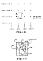
- a fast convolution algorithm using fast Fourier transforms which can be termed a periodic or circular convolution, satisfies the time requirement but treats the image as if it were periodic in both X and Y dimensions.
- Fig. 7 illustrates this effect where the cross-section of a head 46 of a person is illustrated with a wrap around occurring both on the vertical and horizontal axis. Specifically, there is shown in the horizontal axis artifacts of the back portion of the head 47 and the nose 48. Then in the vertical axis there is the nect 49. To eliminate this wrap around effect or artifact it has been suggested in the literature to embed the image and filter in an array of zeroes which contains 4 times the number of points as the original image. This is too time consuming.
- the image sharpening filter process is done by using a hybrid convolution technique which greatly reduces the number of computations and therefore the time for processing.
- Flow Chart 2 illustrates such technique.
- step 51 the border regions of the corrected or restored image are saved. Such border regions are illustrated by the dashed lines 52 in both the horizontal and vertical directions in Fig. 7.
- step 52 the following overall sequence of steps are utilized to form the final sharpened image.
- the restored image of Flow Chart 1 as illustrated in step 51, has its border regions saved. In other words, those regions outlined by the borders indicated at 52. However, at this point there woudl be no wrap around artifact.
- step 52 the image is reconverted back to the Fourier domain.
- step 53 the Fourier domain overall image is multiplied by the SINC function 44 shown in Flow Chart 3, which has been, of course, truncated, and a fast convolution technique well known in the art of the circular or periodic type sharpens the image. Then this image is converted back to the spatial domain, as set out in step 54 to provide the image shown in Fig. 7.
- the border regions are optimally 1/2 filter width so that the truncation of the filter in effect has operated only on the central portion shown by the block 50. Thus, already some wrap around has been avoided.
- step 56 the saved border regions are filtered with the SINC function of step 43 of Flow Chart 3 which is the mollified inverse SINC function in the spatial domain.
- This filtering must be accomplished by a serial convolution technique which inherently takes a longer period of time; however, since it is done only at the border regions, the time is not excessive. And this filtered border region will, of course, contain no wrap around artifacts since, as discussed above, these are only caused by the use of a Fourier transform circular type convolution.
- step 57 the sharpened composite image is formed in the spatial domain by utilizing the inverse transform sharpened image for the central portion of the image and the filtered border regions (done by the serial convolution technique) for the borders of the composite image.
- step 58 the composite image is rescaled (to bring it back to a uniform size) and even negative values are replaced with zero.
- Such negative values may inherently occur during the image sharpening process, which may cause some negative image values which, of course, theoretically cannot be displayed and in any case, are unwanted artifacts.
- a final image is provided as, for example, illustrated in Fig. 7 but without the artifacts.
- the image quality with the use of a 16 neighboring pixels is after sharpening, believed to be superior to the use of 4 neighboring pixels. And lastly, computation time is reduced for the sharpening filter process in using the hybrid convolution technique.
- noise variance must not vary in a visible way as a result of the correction process.
- the noise variance will vary over an 8% range from the 0.46 to 0.50 values. This will still provide an image which does not have the visible artifacts known as "noise streaks.”
- the edges of the image are smoother (less jagged).
- the Gaussian damping factor designated the "alpha" factor of Flow Chart 3, step 41 the signal to noise ratio may be improved as much as 10% without visible blurring of the image.
Landscapes
- Physics & Mathematics (AREA)
- Radiology & Medical Imaging (AREA)
- Nuclear Medicine, Radiotherapy & Molecular Imaging (AREA)
- Health & Medical Sciences (AREA)
- Engineering & Computer Science (AREA)
- Signal Processing (AREA)
- General Health & Medical Sciences (AREA)
- High Energy & Nuclear Physics (AREA)
- Condensed Matter Physics & Semiconductors (AREA)
- General Physics & Mathematics (AREA)
- Image Processing (AREA)
- Magnetic Resonance Imaging Apparatus (AREA)
- Image Analysis (AREA)
Applications Claiming Priority (4)
| Application Number | Priority Date | Filing Date | Title |
|---|---|---|---|
| US94260486A | 1986-12-17 | 1986-12-17 | |
| US07/116,437 US4876509A (en) | 1986-12-17 | 1987-11-03 | Image restoration process for magnetic resonance imaging resonance imaging |
| US116437 | 1987-11-03 | ||
| US942604 | 2001-08-31 |
Publications (2)
| Publication Number | Publication Date |
|---|---|
| EP0272111A2 true EP0272111A2 (fr) | 1988-06-22 |
| EP0272111A3 EP0272111A3 (fr) | 1990-07-18 |
Family
ID=26814243
Family Applications (1)
| Application Number | Title | Priority Date | Filing Date |
|---|---|---|---|
| EP87311100A Withdrawn EP0272111A3 (fr) | 1986-12-17 | 1987-12-16 | Procédé de restauration d'image pour l'imagerie par résonance magnétique |
Country Status (3)
| Country | Link |
|---|---|
| US (1) | US4876509A (fr) |
| EP (1) | EP0272111A3 (fr) |
| JP (1) | JPH01236044A (fr) |
Cited By (5)
| Publication number | Priority date | Publication date | Assignee | Title |
|---|---|---|---|---|
| EP0415683A3 (en) * | 1989-08-31 | 1991-07-31 | General Electric Company | Nmr system |
| EP1246473A1 (fr) * | 2001-03-27 | 2002-10-02 | Koninklijke Philips Electronics N.V. | Appareil de prise de vue comportant un circuit d'amélioration de contour et procédé mis en oeuvre dans un tel appareil |
| EP1582886A1 (fr) * | 2004-04-02 | 2005-10-05 | Universität Zürich | Appareil à résonance magnétique avec des bobines de surveillage de champ magnétique |
| DE102004061507A1 (de) * | 2004-12-21 | 2006-06-29 | Siemens Ag | Verfahren zur Korrektur von Inhomogenitäten in einem Bild sowie bildgebende Vorrichtung dazu |
| EP3804292A2 (fr) * | 2018-06-08 | 2021-04-14 | Tabel, Stefan | Procédé et dispositif de reconstruction de séries temporelles dégradées par des utilisations à capacité maximale |
Families Citing this family (29)
| Publication number | Priority date | Publication date | Assignee | Title |
|---|---|---|---|---|
| JPH03103236A (ja) * | 1989-09-18 | 1991-04-30 | Hitachi Ltd | 核磁気共鳴マルチエコー撮影方法 |
| US5212637A (en) * | 1989-11-22 | 1993-05-18 | Stereometrix Corporation | Method of investigating mammograms for masses and calcifications, and apparatus for practicing such method |
| US5086275A (en) * | 1990-08-20 | 1992-02-04 | General Electric Company | Time domain filtering for nmr phased array imaging |
| US5204625A (en) * | 1990-12-20 | 1993-04-20 | General Electric Company | Segmentation of stationary and vascular surfaces in magnetic resonance imaging |
| US5239591A (en) * | 1991-07-03 | 1993-08-24 | U.S. Philips Corp. | Contour extraction in multi-phase, multi-slice cardiac mri studies by propagation of seed contours between images |
| US5351006A (en) * | 1992-02-07 | 1994-09-27 | Board Of Trustees Of The Leland Stanford Junior University | Method and apparatus for correcting spatial distortion in magnetic resonance images due to magnetic field inhomogeneity including inhomogeneity due to susceptibility variations |
| US5365996A (en) * | 1992-06-10 | 1994-11-22 | Amei Technologies Inc. | Method and apparatus for making customized fixation devices |
| US5748195A (en) * | 1992-10-29 | 1998-05-05 | International Business Machines Corporation | Method and means for evaluating a tetrahedral linear interpolation function |
| US5432892A (en) * | 1992-11-25 | 1995-07-11 | International Business Machines Corporation | Volummetric linear interpolation |
| US5751926A (en) * | 1992-12-23 | 1998-05-12 | International Business Machines Corporation | Function approximation using a centered cubic packing with tetragonal disphenoid extraction |
| US5390035A (en) * | 1992-12-23 | 1995-02-14 | International Business Machines Corporation | Method and means for tetrahedron/octahedron packing and tetrahedron extraction for function approximation |
| US5862269A (en) * | 1994-11-23 | 1999-01-19 | Trustees Of Boston University | Apparatus and method for rapidly convergent parallel processed deconvolution |
| US5682336A (en) * | 1995-02-10 | 1997-10-28 | Harris Corporation | Simulation of noise behavior of non-linear circuit |
| US5726766A (en) * | 1995-07-13 | 1998-03-10 | Fuji Photo Film Co., Ltd. | Interpolating operation method and apparatus for image signals |
| US6137494A (en) * | 1995-08-18 | 2000-10-24 | International Business Machines Corporation | Method and means for evaluating a tetrahedral linear interpolation function |
| DE19540837B4 (de) * | 1995-10-30 | 2004-09-23 | Siemens Ag | Verfahren zur Verzeichnungskorrektur für Gradienten-Nichtlinearitäten bei Kernspintomographiegeräten |
| US5736857A (en) * | 1995-11-21 | 1998-04-07 | Micro Signal Corporation | Method and apparatus for realistic presentation of interpolated magnetic resonance images |
| JP3753197B2 (ja) * | 1996-03-28 | 2006-03-08 | 富士写真フイルム株式会社 | 画像データの補間演算方法およびその方法を実施する装置 |
| US5869965A (en) * | 1997-02-07 | 1999-02-09 | General Electric Company | Correction of artifacts caused by Maxwell terms in MR echo-planar images |
| EP0919856B1 (fr) * | 1997-12-01 | 2005-07-06 | Agfa-Gevaert | Procédé et ensemble pour enregistrer une image radiographique d'un corps allongé |
| US20070055142A1 (en) * | 2003-03-14 | 2007-03-08 | Webler William E | Method and apparatus for image guided position tracking during percutaneous procedures |
| US8303505B2 (en) | 2005-12-02 | 2012-11-06 | Abbott Cardiovascular Systems Inc. | Methods and apparatuses for image guided medical procedures |
| DE102006033248B4 (de) * | 2006-07-18 | 2009-10-22 | Siemens Ag | Verfahren zur Transformation eines verzeichnungskorrigierten Magnetresonanzbilds, Verfahren zur Durchführung von Magnetresonanzmessungen und Bildtransformationseinheit |
| US8970217B1 (en) | 2010-04-14 | 2015-03-03 | Hypres, Inc. | System and method for noise reduction in magnetic resonance imaging |
| US20120013565A1 (en) * | 2010-07-16 | 2012-01-19 | Perceptive Pixel Inc. | Techniques for Locally Improving Signal to Noise in a Capacitive Touch Sensor |
| US8520971B2 (en) | 2010-09-30 | 2013-08-27 | Apple Inc. | Digital image resampling |
| DE102011082266B4 (de) * | 2011-09-07 | 2015-08-27 | Siemens Aktiengesellschaft | Abbilden eines Teilbereichs am Rand des Gesichtsfeldes eines Untersuchungsobjekts in einer Magnetresonanzanlage |
| WO2017134830A1 (fr) * | 2016-02-05 | 2017-08-10 | 株式会社日立製作所 | Dispositif d'assistance au diagnostic d'images médicales et dispositif d'imagerie par résonance magnétique |
| US10698988B2 (en) * | 2017-03-30 | 2020-06-30 | Cisco Technology, Inc. | Difference attack protection |
Family Cites Families (13)
| Publication number | Priority date | Publication date | Assignee | Title |
|---|---|---|---|---|
| GB1594341A (en) * | 1976-10-14 | 1981-07-30 | Micro Consultants Ltd | Picture information processing system for television |
| JPS5481095A (en) * | 1977-12-12 | 1979-06-28 | Toshiba Corp | Computer tomography device |
| JPS57180947A (en) * | 1981-04-30 | 1982-11-08 | Tokyo Shibaura Electric Co | Diagnostic nuclear magnetic resonance apparatus |
| JPS58130030A (ja) * | 1981-10-05 | 1983-08-03 | 工業技術院長 | X線ディジタル画像処理装置 |
| JPS58223048A (ja) * | 1982-06-21 | 1983-12-24 | Toshiba Corp | 磁気共鳴励起領域選択方法、および、該方法が実施し得る磁気共鳴イメージング装置 |
| JPS59148854A (ja) * | 1983-02-14 | 1984-08-25 | Hitachi Ltd | 核磁気共鳴を用いた検査装置 |
| US4579121A (en) * | 1983-02-18 | 1986-04-01 | Albert Macovski | High speed NMR imaging system |
| JPS59155239A (ja) * | 1983-02-23 | 1984-09-04 | 株式会社東芝 | 診断用核磁気共鳴装置 |
| JPS59190643A (ja) * | 1983-04-14 | 1984-10-29 | Hitachi Ltd | 核磁気共鳴を用いた検査装置 |
| US4591789A (en) * | 1983-12-23 | 1986-05-27 | General Electric Company | Method for correcting image distortion due to gradient nonuniformity |
| US4684891A (en) * | 1985-07-31 | 1987-08-04 | The Regents Of The University Of California | Rapid magnetic resonance imaging using multiple phase encoded spin echoes in each of plural measurement cycles |
| US4724386A (en) * | 1985-09-30 | 1988-02-09 | Picker International, Inc. | Centrally ordered phase encoding |
| US4706260A (en) * | 1986-11-07 | 1987-11-10 | Rca Corporation | DPCM system with rate-of-fill control of buffer occupancy |
-
1987
- 1987-11-03 US US07/116,437 patent/US4876509A/en not_active Expired - Fee Related
- 1987-12-16 EP EP87311100A patent/EP0272111A3/fr not_active Withdrawn
- 1987-12-17 JP JP62320059A patent/JPH01236044A/ja active Pending
Cited By (10)
| Publication number | Priority date | Publication date | Assignee | Title |
|---|---|---|---|---|
| EP0415683A3 (en) * | 1989-08-31 | 1991-07-31 | General Electric Company | Nmr system |
| EP1246473A1 (fr) * | 2001-03-27 | 2002-10-02 | Koninklijke Philips Electronics N.V. | Appareil de prise de vue comportant un circuit d'amélioration de contour et procédé mis en oeuvre dans un tel appareil |
| EP1582886A1 (fr) * | 2004-04-02 | 2005-10-05 | Universität Zürich | Appareil à résonance magnétique avec des bobines de surveillage de champ magnétique |
| US7208951B2 (en) | 2004-04-02 | 2007-04-24 | Universitat Zurich Prorektorat Forschung | Magnetic resonance method |
| DE102004061507A1 (de) * | 2004-12-21 | 2006-06-29 | Siemens Ag | Verfahren zur Korrektur von Inhomogenitäten in einem Bild sowie bildgebende Vorrichtung dazu |
| DE102004061507B4 (de) * | 2004-12-21 | 2007-04-12 | Siemens Ag | Verfahren zur Korrektur von Inhomogenitäten in einem Bild sowie bildgebende Vorrichtung dazu |
| US7672498B2 (en) | 2004-12-21 | 2010-03-02 | Siemens Aktiengesellschaft | Method for correcting inhomogeneities in an image, and an imaging apparatus therefor |
| CN1794005B (zh) * | 2004-12-21 | 2010-09-01 | 西门子公司 | 校正图像中非均匀性的方法及采用该方法的成像设备 |
| EP3804292A2 (fr) * | 2018-06-08 | 2021-04-14 | Tabel, Stefan | Procédé et dispositif de reconstruction de séries temporelles dégradées par des utilisations à capacité maximale |
| US12347078B2 (en) | 2018-06-08 | 2025-07-01 | Stefan Tabel | Method and installation for reconstructing time series, degraded by the degree of utilization |
Also Published As
| Publication number | Publication date |
|---|---|
| US4876509A (en) | 1989-10-24 |
| EP0272111A3 (fr) | 1990-07-18 |
| JPH01236044A (ja) | 1989-09-20 |
Similar Documents
| Publication | Publication Date | Title |
|---|---|---|
| US4876509A (en) | Image restoration process for magnetic resonance imaging resonance imaging | |
| EP0280412B1 (fr) | Traitement d'image | |
| US10997701B1 (en) | System and method for digital image intensity correction | |
| US4789933A (en) | Fractal model based image processing | |
| Hwang et al. | Adaptive image interpolation based on local gradient features | |
| US6611627B1 (en) | Digital image processing method for edge shaping | |
| US6701025B1 (en) | Medical image enhancement using iteration to calculate an optimal non-uniform correction function | |
| US7432707B1 (en) | Magnetic resonance imaging with corrected intensity inhomogeneity | |
| US20030198399A1 (en) | Method and system for image scaling | |
| JPH07170406A (ja) | 適応型ディジタル画像信号フィルタ | |
| JPH0879467A (ja) | 高性能画像訂正のための走査線待ち行列化 | |
| CN1109899C (zh) | 三维图象的限带插值法和投影 | |
| US8094907B1 (en) | System, method and computer program product for fast conjugate phase reconstruction based on polynomial approximation | |
| CN101142614B (zh) | 使用各向异性滤波的单通道图像重采样系统和方法 | |
| Seeram | Digital image processing concepts | |
| US7064770B2 (en) | Single-pass image resampling system and method with anisotropic filtering | |
| US7437018B1 (en) | Image resampling using variable quantization bins | |
| US6192265B1 (en) | Diagnostic image processing method | |
| JP3865887B2 (ja) | 画像補正方法 | |
| JPH11309131A (ja) | 医療検査用の画像化方法 | |
| EP4332604B1 (fr) | Appareil de traitement d'image, procédé de traitement d'image et appareil d'imagerie par résonance magnétique | |
| JP2006255046A (ja) | 磁気共鳴映像法および画像処理装置 | |
| US6167414A (en) | System for adjusting size and scale of digital filters and creating digital filters | |
| JP2023103060A (ja) | 画像処理装置、画像処理方法、および画像処理プログラム | |
| JPH06103376A (ja) | 電荷画像走査装置 |
Legal Events
| Date | Code | Title | Description |
|---|---|---|---|
| PUAI | Public reference made under article 153(3) epc to a published international application that has entered the european phase |
Free format text: ORIGINAL CODE: 0009012 |
|
| AK | Designated contracting states |
Kind code of ref document: A2 Designated state(s): DE FR GB IT NL |
|
| PUAL | Search report despatched |
Free format text: ORIGINAL CODE: 0009013 |
|
| AK | Designated contracting states |
Kind code of ref document: A3 Designated state(s): DE FR GB IT NL |
|
| 17P | Request for examination filed |
Effective date: 19900831 |
|
| STAA | Information on the status of an ep patent application or granted ep patent |
Free format text: STATUS: THE APPLICATION IS DEEMED TO BE WITHDRAWN |
|
| 18D | Application deemed to be withdrawn |
Effective date: 19910703 |