EP0466283A2 - Graphisches Anzeigeverfahren - Google Patents
Graphisches Anzeigeverfahren Download PDFInfo
- Publication number
- EP0466283A2 EP0466283A2 EP91202444A EP91202444A EP0466283A2 EP 0466283 A2 EP0466283 A2 EP 0466283A2 EP 91202444 A EP91202444 A EP 91202444A EP 91202444 A EP91202444 A EP 91202444A EP 0466283 A2 EP0466283 A2 EP 0466283A2
- Authority
- EP
- European Patent Office
- Prior art keywords
- trimming
- curve
- trimming curve
- polygon
- patch
- Prior art date
- Legal status (The legal status is an assumption and is not a legal conclusion. Google has not performed a legal analysis and makes no representation as to the accuracy of the status listed.)
- Granted
Links
Images













Classifications
-
- G—PHYSICS
- G06—COMPUTING OR CALCULATING; COUNTING
- G06T—IMAGE DATA PROCESSING OR GENERATION, IN GENERAL
- G06T17/00—Three-dimensional [3D] modelling for computer graphics
-
- G—PHYSICS
- G06—COMPUTING OR CALCULATING; COUNTING
- G06T—IMAGE DATA PROCESSING OR GENERATION, IN GENERAL
- G06T17/00—Three-dimensional [3D] modelling for computer graphics
- G06T17/20—Finite element generation, e.g. wire-frame surface description, tesselation
-
- G—PHYSICS
- G09—EDUCATION; CRYPTOGRAPHY; DISPLAY; ADVERTISING; SEALS
- G09G—ARRANGEMENTS OR CIRCUITS FOR CONTROL OF INDICATING DEVICES USING STATIC MEANS TO PRESENT VARIABLE INFORMATION
- G09G1/00—Control arrangements or circuits, of interest only in connection with cathode-ray tube indicators; General aspects or details, e.g. selection emphasis on particular characters, dashed line or dotted line generation; Preprocessing of data
- G09G1/06—Control arrangements or circuits, of interest only in connection with cathode-ray tube indicators; General aspects or details, e.g. selection emphasis on particular characters, dashed line or dotted line generation; Preprocessing of data using single beam tubes, e.g. three-dimensional or perspective representation, rotation or translation of display pattern, hidden lines, shadows
Definitions
- a typical high performance three dimensional graphics system will describe a surface to be rendered as surface patches defined by functions for each patch. Such functions might be, for example, nonuniform rational B-splines. The use of B-splines imposes certain limitations upon the edges of surface patches.
- B-spline functions Associated with B-spline functions is a normally rectangular uv parameter space. Parametric patch generation functions of u and v compute the values of the coordinates in XYZ space. The rectangular uv space limits the exactness with which the B-spline patch generation functions can represent surface patches having edges of certain shapes. For example, it is difficult to produce a good B-spline description for a patch that is a rectangular region with a circular portion removed from its interior.
- trimming has been performed by the software of the graphics system prior to the sending of device coordinates to the display hardware. Such trimming is necessarily a very complex task, and is generally too slow for use with moving images or interactive systems. It would be desirable to retain the use of B-splines and achieve the advantages offered by that technique of surface description, but at the same time allow high speed trimming.
- trimming is performed on B-spline surface patch descriptions in a hardware graphics accelerator. It receives B-spline descriptions of the patch generation functions for the untrimmed patches and B-spline descriptions of trimming curves in the uv parameter space of the patch generation functions.
- the B-spline descriptions of the trimming curves are themselves functions of a parameter t.
- the graphics accelerator computes a sufficiently dense point by point representation of each trimming curve in uv space, in addition to point by point representations of the individual subspans in uv space whose associated polygons in XYZ space approximate the patch.
- the graphics accelerator determines where straight line approximating segments of the trimming curves cross subspan boundaries and changes the vertices of the subspans to trim away portions of the associated polygon. It does this by building a data structure of linked lists of vertex tables that represent the untrimmed polygon and any trimming curves that cut it. An appropriate traversal of the lists in the data structure produces a list of trimmed polygon vertices in device coordinates. That list may then be further processed to the pixel level by other hardware in the graphics accelerator.
- a mechanism for describing where in a span a trimming curve is located allows the trimming operation to exclude from consideration those trimming curves that cannot possibly affect the polygon being processed.
- Another mechanism compensates for the effects of a non-ideal parameterization of the trimming curve functions, to prevent the production of an unnecessarily high number of polygon vertices.
- the trimming method is also compatible with recursive subdivision of patches to handle patches with a high number of trimming curves.
- Figure 1 is an illustration of a surface in XYZ space approximated by patches formed by mapping spans of a two dimensional uv parameter space into XYZ space with parametric patch generation functions, such as nonuniform rational B-splines.
- Figure 2 shows how a parametric function of a one dimensional t space can define a trimming curve in uv space that in turn can be mapped into XYZ space to identify a region that is absent from the surface.
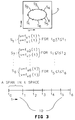
- Figure 3 illustrates a parametric trimming curve function segmented over several spans of the one dimensional t space and defining a trimming curve in the two dimensional uv space.
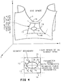
- Figure 4 illustrates how a segmented trimming curve function can cross several spans of uv space to define a mapped trimming curve in a corresponding number of patches in XYZ space.
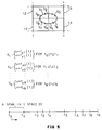
- Figure 5 illustrates the segmented trimming curve of Figure 4 in greater detail.
- Figure 6 shows how the spans in uv space are divided into subspans to produce surface approximating polygons for the surface in XYZ space, and also indicates that the trimming curve in uv space crosses the subspans while the mapped trimming curve trims the polygons on the surface.
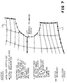
- Figure 7 is an enlarged view of a portion of Figure 6, illustrating the presence of extra vertices along patch boundaries and along mapped trimming curves for better patch-to-patch transitions, and the presence of points along the mapped trimming curve defining points of intersection with the polygon edges as well as approximating points within the interior regions of polygons crossed by the mapped trimming curve.
- Figure 8 is an expansion of a portion of Figure 7 showing how the shapes of polygons are changed by being crossed by a mapped trimming curve.
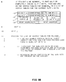
- Figures 9A-C comprise a simplified section of pseudocode describing the processing steps used to produce polygons crossed by mapped trimming curves and whose shapes have been adjusted accordingly, and include an illustration of the structure of a polygon vertex table whose instances are linked together into lists describing polygons.
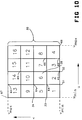
- Figure 10 depicts the order within a span in which subspans are taken to generate the approximating polygons for the surface in XYZ space.
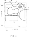
- Figure 11 illustrates several types of trimming curves defined upon a span, and indicates the presence of a guard region around the span to assist in avoiding arithmetic rounding errors.
- Figures 12A-B depict how a clipping mechanism operates upon approximating straight line segments of trimming curves that cross subspans to produce points of intersection between the straight line segments of the trimming curve and the boundaries of the subspan.
- Figures 13A-B describe certain special cases when trimming curves exhibit points in uv space that are very close to the boundaries of the subspan of interest.
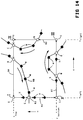
- Figure 14 illustrates a useful example of a subsapn in uv space crossed by certain particular trimming curves, and serves as the basis of an explanation of how the linked boundary list of vertex tables and its linked trimming curve sublists are traversed to produce polygons that are present ON the surface.
- Figure 15 is a simplified schematic representation of a linked boundary list and trimming curve sublists for the vertex tables corresponding to the example of Figure 14.
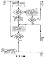
- Figures 16A-C comprise a simplified flowchart for processing the linked list of vertex tables in accordance with step 12 of Figure 9C.
- Figure 17 is a simplified section of pseudocode pertaining to the same subject matter as Figures 16A-C, but with more detail concerning the structure of the vertex tables shown in Figure 9B and Figure 15.
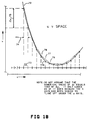
- Figure 18 is a diagram of a trimming curve in uv space illustrating a refinement in the selection of points in uv space representing the trimming curve in the operations of clipping and trimming.
- Figure 19 is a simplified hardware block diagram of the component instruments used in an embodiment incorporating the preferred method of the invention.
- Figures 20A-C comprise a simplified hardware block diagram of the graphics accelerator of Figure 19.
- a three dimensional surface may be represented within a graphics system.
- a saddle-shaped surface 1 such as the one depicted in Figure 1 were to be represented. This would be accomplished by dividing the entire surface 1 into smaller portions (commonly called patches), of which the patch 2 is illustrative. To adequately render a surface as complicated as the saddle shape 1 a great many patches would be required.
- the graphics system would include some means to divide the surface into appropriate patches.
- the various other curved lines in Figure 1 are not there to suggest other patches (although they might), but are instead offered as an aid in appreciating the shape of the surface 1.
- the surface 1 resembles a hyperbolic paraboloid, the method to be described is particularly applicable to irregular ("free-form") surfaces, especially those rendered from parametric B-spline descriptions.
- the portion is called a span.
- a two dimensional paramenter space is employed.
- the two paramenters are u and v, and each is allowed to vary between associated maximum and minimum values.
- a set of parametric patch generation equations 4 map values in the parameter space 3 into XYZ space to produce the (X,Y,Z) triples that lie on the patch 2.
- a modern high performance graphics system will store a complete description of the object, independent of any particular view that may be desired. Often this description takes the form of a data base, particularly when subportions of the object are described separately and then deployed by reference, perhaps a multiplicity of times. Rather than store in the database an exhaustive collection of points on the surface it is common to instead employ a more compact type of description, such as approximating functions that yield values to a desired degree of resolution. When a particular view is wanted it is found by computing translations and or rotations for points first found by evaluation of the approximating functions in the database. B-splines are a technique for achieving such a compact representation through parametric functions.
- Figure 1 illustrates that each point 6 on a surface of interest 1 can be represented by a corresponding point 7 in some portion 5 of a parameter space 3.
- the user of the graphics system interacts with that system in defined ways set out in an operating manual for the system.
- a desired surface may be constructed.
- the surface will be composed of a multiplicity of patches.
- the internal activities of the graphics system produce three (or perhaps four) patch generation functions of u and v.
- the variables u and v belong to the parameter space 3.
- the x coordinate of the point 6 is found by evaluating a (polynomial) function F x (u,v).
- Corresponding functions F y and F z produce the y and z coordinates of the point 6.
- each of the functions F x , F y and F z has been rationalized through division by the function H.
- the method to be described is compatible with either rational or nonrational nonuniform B-spline representations.
- the parameter u is allowed to range in equal steps from u min to u max , while the parameter v ranges in equal steps (not necessarily the same as those for u) from v min to v max .
- This evaluation of the span produces "raw" polygon vertices that are generally subjected to a fair amount of further processing prior to being displayed.
- the surface to be displayed is described as a collection of patches, each of which has an associated span. Associated with each span is a particular collection of B-spline patch generation functions.
- the method of the invention affords a solution to the problem of complex surfaces that do not have practical B-spline descriptions.
- the hole in the plate has an edge in XYZ space
- there are corresponding points in uv space which, when evaluated, will exactly describe or closely approximate the edge of the material to be removed to produce the hole. These points lie along a curve in uv space, called a trimming curve.
- the trimming curve can be represented by one or more functions. These functions can be found by the solid modeling package. Thereafter, the rendering of a patch having a "subtracted" portion can be accomplished by a qualified evaluation of the patch generation functions for the associated span.
- the qualification takes the form of determining, during the evalualtion of the patch generation functions, whether the (u,v) pair at hand lies on, inside or outside of the timming curve.
- the qualification produces a decision about whether or not to display the associated (X,Y,Z) triple. If that triple is to be displayed, things proceed as previously described. However, if the evaluation of that (u,v) pair would produce a polygon vertex lying within the region to be subtracted, then the triple cannot be displayed and the existing polygon structure must be modified.
- Figure 2 illustrates the use of a trimming curve 8 to describe the boundary in XYZ space of a region 9 to be subtracted from patch 2.
- the trimming curve 8 is defined in a span 5 of the parameter space 3.
- the trimming curve 8 can itself be defined by B-splines.
- a pair of parametric equations 9 of a parameter t can define a two dimensional trimming curve in uv space.
- trimming curve functions 9 can be either rational or nonrational non uniform B-splines.
- a trimming curve must generally be piecewise assembled from subportions called segments. Each segment has its own particular trimming curve functions 9.
- Figure 4 describes a generalization of the application of trimming curves. What is shown is similar to the situation depicted in Figures 2 and 3, but with the difference that the trimming curve 11 now traverses several spans 12-15 in uv space. This situation arises because, as luck would have it, the portion 9 to be subtracted from the surface 1 occupies the four corresponding patches 16-19.
- the segment boundaries of the trimming curve 11 are shown on that curve in Figure 4. Note that, in general, the boundaries between the segments S1 through S9 may fall anywhere along the trimming curve 11. In particular, they need not have any special relationship to the boundaries between the spans 12-15.
- Figure 5 depicts the piecewise representation of the segmented trimming curve 11 of Figure 4. Note the use of different parametric equations for each segment, and that each set of those equations is defined over it own associated span in t space 20.
- Figure 6 shows four spans 12-15 that map, according to the heavy arrows, into the four patches 16-19. Each of the spans is traversed by a trimming curve 11, whose purpose is to define the trimmed (or "subtracted") region 9 in the resulting surface.
- a trimming curve 11 whose purpose is to define the trimmed (or "subtracted") region 9 in the resulting surface.
- the process of generating the patches is carried out one patch at a time. Accordingly, spans are evaluated one at a time; each span produces one associated patch.
- the evaluation of a span involves the determination of step sizes for u and v. These step sizes are not necessarily the same for u and v, and each is again determined upon beginning the evaluation of the next span. That is, the step sizes delta u i and delta v i for span 13 need not be equal to each other, nor need they bear any relationship to the step sizes delta u j and delta v j for span 12. In particular, there is no requirement that delta u i equal delta u m or equal delta u n , even though for simplicity they appear to be equal in the figure. A similar statement applies to the delta v's.
- the user of the graphics system will have at least indirect control over the step sizes. In some systems it may be possible for the user to specify them directly, although it is more likely that the specification is arrived at indirectly. For example, the user may instruct the graphics system to choose step sizes such that the resulting polygon edges have approximately a particular number of pixels. Bear in mind that, in general, the step sizes can be redetermined afresh for each span.
- the selection of step sizes for a span determines a collection of (u,v) pairs within that span. This is represented by the dotted lines withing the spans 12-15.
- the intersections of the dotted lines with themselves, and of the dotted lines with the solid lines representing the boundaries of the spans, are the points at which the patch generation functions are evaluated. For example, the evaluations of the patch generation functions at point 21-23 produces polygon vertices 24-26.
- Trimming is a fairly complicated process, requiring the analysis of several possible situations.
- a given vertex may belong to a polygon that is totally unaffected by trimming, one that is to be trimmed away in its entirety, or, to one that is crossed by the trimming curve. In this latter case part of the polygon remains and part of it does not.
- This requires changing the shape of the polygon to match the trimming curve. That, in turn, will require the finding of new vertices for that polygon; ones that were not produced by the evaluation of the span at the steps in u and v as shown in Figure 6.
- mapped trimming curve we mean the trimming curve 11 as mapped into the patches by the patch generation functions.
- FIG. 7 Two kinds of polygon vertices along patch boundaries are shown in Figure 7.
- the open circles correspond to the mapping into the patches of: a) the points of intersection of the dotted lines of Figure 6 with the span boundaries, and b) the points of intersection of the dotted lines with themselves.
- the closed circles correspond to "extra" vertices that are added by evaluating additional (u,v) pairs along the span boundary. These extra points divide each step of delta u into equal subportions; the steps of delta v are similarly divided. It is common for the user to have some degree of control over the process of adding these extra vertices.
- Figure 7 also shows polygon vertices along the mapped trimming curve 27. It is clear from an examination of the figure that a good many extra vertices have been added to the polygons as part of the trimming process. We shall have much to say about this, and turn now to Figure 8, which is a further expansion of that portion of the mapped trimming curve 27 pertaining to patch 17.
- Segments S6 through S8 are evaluated by finding, for each segment, a delta t that ideally produces steps in u and v that are each roughly equal to the distance, in uv space, between the points along the span boundary that correspond to an open circle and its nearest solid black circle neighbor on patch boundaries of Figure 7.
- This business of selecting the delta t's is influenced by the user's choices made in connection with extra vertices for patch boundaries. In reality (and in contrast with the ideal case), the evaluation of the trimming curve 11, as described above, produces many (u,v) pairs that are spaced too close together to be useful.
- a further refinement is to examine the pairs produced by the evaluation of the parametric functions (for the example at hand these are F u6 & F v6 , F u7 & F v7 , F u8 & F v8 ) and suppress pairs that are insufficiently distant from their predecessors.
- the solid black squares of Figure 8 result from evaluating the patch generation functions at these refined (u,v) pairs.
- the second thing that is of interest in Figure 8 is the open squares. These represent the intersection of the mapped trimming curve 27 and the polygon edges. Rather than find the intersections in XYZ space, the corresponding point of intersection is found in uv space and then mapped into XYZ space. Specifically, what is found is the intersection of two straight line segments in uv space. One of the straight line segments is between two consecutive refined (u,v) pairs along the trimming curve 11. The other straight line segment would be a portion (e.g., 28 or 29 in Figure 6) of the dotted lines or span boundaries of Figure 6.
- Figure 9 That figure is a simplified pseudocode description of activity performed by a transform engine portion of a high performance graphics system hardware apparatus. That hardware apparatus is the subject of description that appears in a later portion of this Specification and its Figures. The activity mentioned above is primarily the trimming of polygons as illustrated in Figure 8.
- Figure 9 may be understood as a condensed road map for accomplishing the type of trimming described in connection with Figure 8.
- the graphics system is capable of displaying several B-spline surfaces, each of which may be variously trimmed. Each surface would generally be composed of a plurality of patches. The trimming activities occur at the level of polygon handling within each patch. Accordingly, steps 1 and 2 (in conjunction with steps 15 and 16) of Figure 9 apply the process to be described in connection with steps 3-14 to each of the patches in all of the surfaces.
- Step 2 is accomplished in software executed by the computer associated with the graphics system. Among other things, step 2 divides the surface into patches, selects a patch to be rendered, computes u min , u max , v min , and v max for the associated span, and decides which segments of which trimming curves will be needed for trimming the patch.
- Steps 3-14 generate trimmed polygons vertices that can be displayed by a polygon rendering mechanism in the hardware of the graphics system.
- That activity includes the primary generation of the various polygons (as indicated by steps 3 and 14), and their subsequent (and immediate) trimming (as indicated by steps 4 through 13).
- the general order of polygon generation within a patch is illustrated in the example span 30 of Figure 10. That span is partitioned, in this example, into sixteen subspans; one for each untrimmed polygon to be generated. The size of each subspan is determined in accordance with the user's instructions pertaining to the desired visual smoothness of the surface.
- the polygons are generated by a technique called forward differencing, which does not require the explicit calculation of the u and v values for the boundaries of each of the subspans. Forward differencing is preferred because it is faster than evaluating the patch generation functions at each of the subspan corners. For a description of forward differencing see Foley and Van Dam, pages 535-536.
- clip limits refers to a window of interest. Objects within the window are retained, while those that fall outside are discarded.
- the clip limits that will be of interest to the trimming described herein are the subspan boundaries in uv space that are associated with the generated polygons.
- Step 4 computes the clip limits (in uv space) for the polygon currently being generated and trimmed.
- Figure 9A includes a subspan 35 having clip limits u left , u right , v top and v bottom .
- Subspan 35 could, for example, correspond to subspan A6 in Figure 10: u left would be the value 31, u right would be the value 32, v top would be the value 34, and v bottom would be the value 33.
- finding the clip limits for the various subspans requires determining the u values 31, 32, ... and v values 33, 34, ... that partition the u and v axes.
- these are 32-bit floating point binary numbers.
- a preferred method described next, allows the polygons to be generated at separate times while ensuring, by saving certain principal values of interest, that common corners have identical u values and identical v values.
- Step size values are found as previously described. While traversing a row (say, from subspan A2 to subspan A3) the u right of subspan A2 is saved and reused as the u left of subspan A3. At the beginning of a row u min for the span is taken (exactly) as u left . Along a row a new u right is found by adding delta u to the old value of u right . At the end of the row u max for the span is taken (exactly) as u right . The values u min and u max arise when the B-spline generation software segments a surface into patches (see Figure 1).
- v min Upon starting the first row v min is taken (exactly) to be v bottom .
- the value for v top is found by adding delta v to v bottom .
- the old value of v top is saved and reused as the new v bottom .
- the new v top is found by adding delta v to the old value of v top .
- Step 5 (in conjunction with step 10) of Figure 9A may be better understood with reference to Figure 11. That figure shows a span 36 crossed by a number of associated trimming curves 37-40. Recall that trimming curves are generally defined as segmented B-splines. When considering what actions to take in trimming a particular patch, only those trimming curve segments that are inside the associated span need be considered. In accordance with what was said in connection with step 2 of Figure 9, a mechanism in the software of the graphics system will associate one or more lists of trimming curve segments with each span.
- Open trimming curves must start and end outside of their associated span.
- the number of trimming curve segments to be included in a list for an open trimming curve will be increased to include starting and ending segments that are "clearly" inside the span or "clearly” outside the span, beyond any possible doubt or error that could be introduced by roundoff errors. This may be accomplished, for example, by considering the span to be, say, five percent bigger than it really is, as shown by the dotted line 41.
- step 6 of Figure 9 which (in conjunction with step 9) concerns the notion of straight line segments along a trimming curve.
- the task of trimming is going to involve finding many points along each trimming curve.
- Figure 8 all of the open and solid squares along the mapped trimming curve 27 have to be found (locally, as it were) as a part of the trimming process.
- the "straight line segments" of step 6 of Figure 9 correspond to straight lines between the solid squares of Figure 8.
- Implicit in step 6 is the finding of (u,v) pairs which, when evaluated by the patch generation functions 4, will produce the solid squares. It is the finding of those (u,v) pairs that is of interest at the moment.
- (u,v) pairs along the trimming curve having approximately the same spacing therebetween as the extra vertices added to the span boundaries for polygon generation. That is, the steps in u along the trimming curve should be no larger than the distance in u between the extra vertices. If there are no extra vertices, then the maximum distances should be taken as the distance between corner vertices. A similar requirement applies to steps in v along the trimming curve.
- This collection of (u,v) pairs is a separate collection of points different from any other, say, that used for polygon generation.
- the steps along the trimming curve will correspond to the solid squares of Figure 8. They will be used to determine additional (u,v) pairs that correspond to the open squares of Figure 8. We now describe how the initial steps along the trimming curve are found.
- the basic idea is to evaluate each segment of each trimming curve at some selected (and manageably small) number of points.
- the largest of the resulting increments in u and the largest of the resulting increments in v are each saved. These increments are compared to the respective distances in in and v between the extra vertices along patch boundaries. If the comparison is favorable the desired step size in t has been found. If the comparison is unfavorable, then the step size in t is adjusted in accordance with the ratio of the largest resulting step size and the desired step size.
- This determination process is performed separately for u and v, resulting in two candidates for a stepsize in t. The smaller of the two stepsizes is selected.
- Step 7 in Figure 9 may be understood with reference to Figure 12 and an appreciation of the Cohen & Sutherland clipping algorithm.
- Figure 12A depicts a straight line segment 42 (having a direction that is from P1 to P2) that crosses a clip window 43 of interest.
- the purpose of finding a uniform step size in t and using the forward differencing to evaluate the trimming curve function (in the direction of increasing values of t) is to find a sufficient number of points along the trimming curve. These points are the solid squares of the figures, and the directed straight line segments between them are a close approximation of the ideal trimming curve described by the B-spline functions.
- Clipping finds the points of intersection (if there are any) between each staight line segment 42 and the clip window 43. This allows the determination of exactly what part 44 of the staight line segment 42 lies within the clip window 43.
- part 44 is the line between NEWP1 and NEWP2.
- NEWP1 and NEWP2 are computed by the clipping process. The subscripts indicate that the line segment 44 has a direction.
- the trimming method to be described uses the notion of directed motion along the trimming curves. Simply put, as you travel along the trimming curve (or its straight line approximation) the stuff on the right gets trimmed away.
- a given trimming curve may produce one or more tables to be added to the list. Because trimming curves have a direction associated with them (increasing values of t), it is useful to distinguish among: a) points of intersection along the boundary of a clip window where a trimming curve enters the window; b) points along a trimming curve that are inside the clip window; and c) points of intersection along the boundary of a clip window where a trimming curve leaves the window. These points will be called “BEGIN”, “MIDDLE”, and "END” points, respectively. In general a clip window can be cut by several trimming curves. It is desirable group the tables for each individual trimming curve into separate circularly linked sublists within the larger list of all of the tables generated for a particular clip window.
- the general format of the tables is shown in Figure 9.
- the first two entries 45 and 46 in a table are the binary floating point values of the u and v coordinates for the point of interest (either NEWP1 or NEWP2).
- the third entry 47 contains three parts: either zero or a nonzero trimming curve number (an 8-bit integer); either zero or a nonzero B-spline segment number (also an 8-bit integer) identifying the trimming curve on which the point in uv space lies; and six flag fields. (Zeros in the first two parts indicate special cases described later in a more detailed description of a preferred implementation.)
- the six flag fields are:
- the fourth entry 48 contains the Wrap Address and the Next Address.
- Nonzero Wrap Addresses are the circular links in an otherwise linear (i.e., physically ordered) list of tables.
- a Wrap Address of zero indicates that the next physical table is also the next logical table in the list.
- Tables are inserted onto the end of the list of tables in an orderly manner as trimming curves are traversed in the direction of increasing values of t. To make the desired circularly linked sublist for a trimming curve it is merely necessary to insert the address of the first table for that trimming curve into the Wrap Address of the last table for that trimming curve.
- the Next Address is determined by steps 11 and 12 in Figure 9. It links the tables into another list used to display portions of polygons that are present.
- step 8 of Figure 9 it is appropriate to describe the criteria used to build the list of tables in response to information provided by the clipper.
- the criteria used to build the list of tables in response to information provided by the clipper.
- the following decision tables describe how this is done. In these decision tables the flag INSIDE is used to remember if P2 is inside or outside the clip window.
- Steps 9 and 10 cooperate with steps 6 and 5, respectively, described above.
- the result of these nested FOR loops is the division of each timming curve into straight line segments. Those are then clipped by step 7 against the subspan whose polygon is to be rendered. Step 8 builds a list of tables describing the clipped straight line segments.
- steps 11(a)-(d) the list of tables produced at step 8 is processed in four ways. The first of these is an inspection by step 11(a) for the two special cases shown in Figures 13A-B.
- FIG. 13A what is shown there is a subspan 49 and a trimming curve 50 having a point 51 that falls "just outside” the clip window.
- a point of intersection 52 will be calculated for where the trimming curve 50 "goes out” of the clip window 49.
- the trimming curve comes right back in again.
- the clipper will dutifully produce another point of intersection 53.
- the point 51 is sufficiently close to the clip limit (which in the example is the right-hand edge, but it could be any edge) the finite resolution of the numbers used in the calculations can result in both the exit and entrance points lying on top of one another.
- the clip limit which in the example is the right-hand edge, but it could be any edge
- the finite resolution of the numbers used in the calculations can result in both the exit and entrance points lying on top of one another.
- FIG. 13A is all about; within the degree of arithmetic precision in use, points 52 and 53 are the same point . This is really what we mean by "just barely" outside.
- the first will be an END table (see FF1 in connection with step 8 of Figure 9) and the second will be a BEGIN table. Furthermore, both tables will have exactly identical u values and exactly identical v values.
- This state of affairs is the first special case associated with the processing of the list of tables by step 11(a). The first special case is found by inspecting each of the circularly linked sublists associated with the trimming curves. If any sublist contains logically adjacent (i.e., with the Wrap Address taken into proper account to produce correct logical ordering) BEGIN and END tables each containing the same identical (u,v) pair, then each of those tables is converted to a MIDDLE table.
- the second special case that is checked for is depicted in Figure 13B.
- This case is generally analogous to the first special case, except that the trimming curve 54 extends "just barely" into the clip window 55.
- the finite resolution of the numbers used in the calculation of points of intersection will produce a BEGIN table and an END table for points 56 and 57 having the same (u,v) pair.
- the BEGIN and END tables will be separated by a MIDDLE table for point 58.
- step 11(a) The second special case is found in step 11(a) by an inspection of the list for sublists containing BEGIN - MIDDLE - END sequences having BEGIN and END tables containing the same identical (u,v) pair.
- the SKIP flag (refer to step 8 of Figure 9) is set in all three tables. The net effect of this upon later processing of those tables is their effective deletion; they are simply ignored.
- step 11(b) the list of tables is processed to make four new sublists; one sublist for each edge of the clip window, with each such sublist enumerating the trimming curves which cross the assoicated edge.
- These new edge sublists are formed in place, as it were, by using the NEXT ADDRESS field of the tables to link the edge sublists together. (This will be only an intermediate use of the NEXT ADDRESS field, not its final use.)
- edge sublists Only BEGIN and END tables without their SKIP flags set are included in the edge sublists. In forming the edge sublists special attention will be paid to cases where the (u,v) pair in a BEGIN or END table is also a corner point of the clip window. In this connection it will be helpful to refer now to Figure 14, which depicts a clip window crossed by several trimming curves.
- a BEGIN or END table whose (u,v) pair also (by chance) describes the corner point I goes into the edge sublist for the top edge 59.
- a BEGIN or END table at corner II goes with the left edge 60.
- a BEGIN or END table at corner III goes with the bottom edge 61.
- a BEGIN or END table at corner IV goes with the right edge 62.
- each edge sublist is sorted by either ascending or descending values of either u or v, depending upon which edge the sublist represents.
- the attributes BEGIN and END do not influence the sorting.
- the edge sublist for the left edge is sorted according to decreasing values of v.
- the edge sublist for the bottom edge is sorted according to increasing values of u.
- the edge sublist for the right edge is sorted according to increasing values of v.
- the edge sublist for the top edge is sorted according to decreasing values of u.
- the list of tables is processed to interleave the four edge sublists with tables in the main list for corners and extra vertices to produce a new circular ordering in the list.
- This is the final use of the NEXT ADDRESS field.
- the interleaving begins (arbitrarily) with corner vertex I, and proceeds counterclockwise around the boundary of the clip window.
- the NEXT ADDRESS field of each table for a point along the boundary is linked to the next point further along the boundary, whether that be an extra vertex, or an intersection with a trimming curve. It could even be the case that the next vertex is the next corner.
- This reordering is represented in Figure 14 by the arrows connecting the points labeled as C's, X's, B's and E's. Beginning arbitrarily with vertex I, the resulting ordering is C-X-E-X-X-C-X-B-X-E-C-B-C-E-B-C.
- the only types of tables included in this reordering with the NEXT ADDRESS field are corners, extra vertices, and the BEGIN and END intersection point tables; left undisturbed are the sublists for each trimming curve enumerating the points along each trimming curve within the clip window (the MIDDLE's between the BEGIN's and END's).
- Step 11(d) of Figure 9 calculates the ON flag for each table in the circularly linked list just descirbed above in connection with Figure 14 and step 11(c) of Figure 9.
- the ON flag indicates if a vertex remains present ON the surface or is trimmed away. What interests us here is how the ON flag may be calculated. Simply put, this is done by finding a point where a trimming curve leaves the subspan. By definition, every point on a trimming curve is assumed to be present. Trimming involves the further assumption that everything in a subspan that is to the left of the trimming curve (while proceeding along the trimming curve in the direction of increasing t) is also present.
- the circularly linked list for a subspan contains no BEGIN or END tables. This can happen in two different ways. First the subspan might have no trimming curves associated with it at all. Such a subspan will have only tables for corners and extra vertices. In the second case a subspan might wholly contain one or more trimming curves. (These might touch or coincide with the subspan boundaries, but not cross them, and the effect will be the same when the curve is entirely inside without touching.) Such a subspan will give rise to a list having tables for corners, extra vertices and MIDDLE's for the trimming curve(s).
- the trimming curve is smaller than the smallest "unit of interest" (i.e., the polygon). The trimming curve will be ignored and the entire polygon tentatively retained. However, it does not necessarily follow that the polygon will remain present; it might itself be within a larger trimming curve, and so be trimmed away.
- the presence of the polygon will depend upon the presence of adjoining polygons.
- step 11(c) it was said that the four edge sublists were interleaved counterclockwise around the subspan, beginning with vertex I.
- a trimming curve crosses a boundary by passing through vertex I 67 there are in the circularly linked list actually two tables describing vertex I; one for vertex I itself and one for the BEGIN or END coincident with vertex I.
- Each of those tables has an ON flag; special attention must be paid to how to interpret these in light of the rules by which they were set and the special case at hand.
- vertex I will be marked OFF (absent).
- the adjacent patch above the current patch is, by rule 2, ON (present).
- the value of the ON flag for vertex I 67 propagated to the next patch needs to be changed from OFF to ON.
- vertex I will be marked ON.
- the adjacent patch above the current patch is, by rule 2, OFF.
- the value of the ON flage for vertex I 67 propagated to the next patch needs to be changed from ON to OFF.
- the general rule for propagating the ON flag for vertex I 67 of the first subspan of the last row is: if there is in no BEGIN or END coincident with vertex I 67, propagate the unchanged value of the ON flag for vertex I 67. If there is a BEGIN or END coincident with vertex I 67, propagate the complement of the value of the ON flag of vertex I 67.
- a specific rule is needed to calculate the ON flag for the very first vertex of an entire surface. Such a rule amounts to a convention, but should be consistent with the trimming operations that might apply to that very first vertex. For example, assuming that the very first vertex is always present ON the surface might not allow that vertex to be trimmed away.
- a convenient rule for the calculation of the ON flag of the very first vertex is to require that surface edges or portions thereof that are present (ON) are bounded by a trimming curve. With this approach the very first vertex can be assumed to be OFF.
- step 12 of Figure 9. Its task is to traverse the list of tables. Step 11 added to the list information about what original vertices remain present after trimming, as well as what trimming curve vertices are to be incorporated into the trimmed polygon. Note that step 11 may have effectively divided the original polygon into two or more smaller polygons.
- Step 12 uses a simple procedure of nested loops to traverse the data structure prepared by step 11. A simplified representation of how that data structure would represent the situation of Figure 14 is depicted in Figure 15.
- the result of the traverse by step 12 is sequences of present polygon vertices that are sent by step 13 to a mechanism for actually displaying the polygons. Step 12 will produce one complete list of vertices for each present polygon or present subpolygon (a part of a polygon remaining after another part has been trimmed away) emerging from the trimming process.
- Figure 15 is simplified illustration of one possible circularly linked list of vertex tables that could result from applying step 11C of Figure 9B to the example of Figure 14.
- the entire circularly linked list of Figure 15 may be termed a boundary list.
- the Next Address field links untrimmed polygon vertices and points of intersection between the polygon edges and the trimming curves into the boundary list.
- Embedded within the boundary list are trimming curve sublists.
- the trimming curve sublists are linked by a combination of physical ordering and the Wrap Address field. There is one trimming curve sublist for each trimming curve.
- a choice can be made to either continue along the boundary list or to switch over to traversing the trimming curve sublist. (The boundary list and the trimming curve sublist share BEGIN and END tables; to switch all that is needed is to follow the other chain of links.) If a trimming curve sublist is traversed to its END, the boundary will be reentered at that point.
- Step 12 is depicted in Figure 16 as a simplified flowchart, and in Figure 17 as pseudocode for operating upon the list of tables containing the information set out in step 8 of Figure 9.
- FIG. 16 The flowchart of Figure 16 is believed to be fairly self-explanatory when taken in the context of what has preceded it. It includes an outer loop, shown in Figure 16A, that selects an arbitrary vertex in the circularly linked boundary list as an initial vertex that it then marks as having been "first". The outer loop then traverses the boundary list. When it discovers that it has gotten back to the vertex marked "first", the process is complete, and the loop terminates.
- the main activity of the outer loop is to identify vertices that have not yet been visited and that are on the surface. When such a vertex is found it location in the boundary list is saved, so that the outer loop can resume traversing the list at this point after the middle and inner loops have been allowed to traverse the list on their own. With the outer loop thus "suspended", as it were, further processing of the list by the middle loop commences.
- the middle loop adds to a polygon list any present non-timming curve vertices and identifies a BEGIN or END vertex.
- a BEGIN vertex is found it is added to the polygon list and the inner loop is then entered.
- An END vertex is also added to the polygon list because it is a next vertex present ON the polygon, and because it has now been marked as visited, and will not be further processed if it is visited again.
- the inner loop traverses a trimming curve sublist whose head has been reached by traversing along the boundary list with the outer and middle loops.
- the middle loop enters the inner loop after adding a BEGIN vertex to the polygon list; the inner loop returns to the middle loop when the balance of the trimming curve sublist has been entirely traversed and the associated vertices added to the polygon list.
- the middle loop then resumes its traverse of the boundary list.
- the inner loop is re-used as needed each time the head of a new trimming curve sublist is encountered.
- the middle loop will complete itself when an entire closed polygon has been added to the polygon list. This condition is detected when the middle loop returns to a vertex that has already been visited. This does not necessarily mean that the boundary list has been fully processed; trimming can cut an original polygon into two or more subpolygons. As long as the outer loop has not yet run to completion there may be more subpolygons described by the boundary list.
- the middle loop Upon the addition of a complete polygon to the polygon list the middle loop returns to the outer loop. It resumes its processing at the point in the boundary list where it left off. It continues to traverse the list looking for vertices that have not yet been visited. If it finds one it re-uses the middle loop to put another entire subpolygon onto the polygon list.
- vertex information is substantially easier to add vertex information to the polygon list for corner and extra vertices (operation 69 in Figure 16) than it is for points along trimming curves (operations 70 and 71 in Figure 16).
- the former information is computed, as mentioned previously, by the forward differencing technique.
- the latter information involves evaluating, for abritrary points in uv space, the vertex position in XYZ space and the surface normal vector at the vertex. While not conceptually difficult, this is a much more time consuming operation.
- Figure 17 is a simplified section of pseudocode to perform the same activity as set out in flowchart form in Figure 16. The difference is that Figure 17 incorporates more of the table structure described in connection with steps 8-11 of Figure 9.
- a step size in t (delta t) is selected to produce maximums for delta u and delta v that are about equal to the distance between polygon vertices along the edge of the patch, which distance may be termed the edge step size. That is how the delta t 73 of Figure 18 is selected. For the purpose of illustration, assume that the largest delta v 75 shown in Figure 18 was used to determine delta t. In the illustraton at hand the delta v's tend to be bigger than the delta u's. For a different trimming curve it might be the case that the largest delta u exceeds the largest delta v and would be used to select delta t. The process of selecting delta t is described in connection with step 6 of Figure 9.
- the straight line segment approximation of the trimming curve 72 that it obtained by evaluating it functions at the equal step sizes of delta t 73 is refined by requiring that at least one of delta u and delta v exceed fifty-two percent of the edge mesh size. If neither does then that point in uv space is ignored, and the next one is considered, and so on. According to this technique, point 76 would be ignored, and straight line segment 77 would run from point 78 to point 79.
- the first point along each B-spline trimming curve segment is the initial point at which the point selection process begins. This ensures that the B-spline trimming curve segments join each other as intended.
- the fifty-two percent criterion arises from a relationship that exists between the shortest and longest accepted straight line segments.
- the relationship involves an equality between the amount that a longest accepted straight line segment (one at forty-five degrees) exceeds the edge step size on the one hand, and the amount the shortest accepted straight line segment (one that is horizontal or vertical) is less than the edge step size on the other hand. It may be shown that the desired equality relationship obtains when the selection criterion is approximately fifty-two percent of the edge step size.
- the number of trimming curves that must be considered while processing a subspan and its polygon may be reduced by use of the following technique. Simply put, information about the location of each trimming curve segment within the span is associated with its B-spline definition. This information is used to eliminate from consideration those segments that cannot possibly intersect the subspan about to be processed.
- a v extent is found for each B-spline segemt of each trimming curve.
- the v extent is the range in v from the minimum v value to the maximum v value in the set of (u,v) pairs resulting from the parameterization refinement described in connection with Figure 18.
- the u extent mentioned below is defined similarly.
- the vextent for each B-spline segment is stored in a location within a data structure containing the trimming curves for the patch.
- trimming curve segment 80 would not be of interest for any subspan/polygon in row 82 of patch 12; segment 80 does not have a v extent that overlaps the v extent of row 82.
- the v extent of segment 81 does overlap that of row 82, and the u extent of segment 81 is computed prior to processing any of the supspans along row 82.
- segment 81 overlaps the u extent of the subspan 83, the B-spline segment 81 of trimming curve 11 is included in the clipping and trimmng activities for that subspan.
- Segment 80 would not be included in the activities for any subspan/polygon along row 82, nor would it, for further example, be used in connection with subspan 84. And in the same manner, neither segment 80 not segment 81 would be included in the activities for any subspan/polygon along row 85; no v extent for those segments overlaps that for the row.
- the graphics system includes a computer 86, a keyboard 87, a knob box 88, a button box 89 and a mouse 90.
- the computer 86 may execute the software, mentioned at the beginning of this Specification, which interacts with the user and prepares the B-spline descriptions of the surface and its trimming curves.
- the computer 86 is coupled to a grahics accelerator 91 through a high speed local graphics bus 92.
- the graphics accelerator 91 is in turn coupled to a color monitor 94 through three coaxial cables for carrying the Red, Green and Blue (RGB) video signals.
- RGB Red, Green and Blue
- the trimming activities described above are performed entirely within the graphics accelerator 91. While it is conceivable that the trimming method that has been described could be carried out in software in the computer 86, such an approach necessarily incurs a substantial penalty through reduced performance compared with trimming by appropriate hardware.
- the graphics accelerator 91 is responsive to the computer 86 through the execution of a number of commands. Among these are some that: instruct the graphics accelerator to store in a data structure the definition of one or more trimming curves; store in a data structure a surface patch definition and then render it with trimming according to the previously defined trimming curves; and a command to delete all previously defined trimming curves. Also included are commands to push and pop a stack of ON flags.
- the ON flags for the upper right and lower left corners of selected patches are saved on two separate stacks to facilitate the subdivision of patches.
- the subdivision of patches into subpatches arises when a given patch contains too many trimming curves; there are practical and cost related considerations (i.e., the amount of memory) that limit the number of trimming curves for any single patch that can be handled by the graphics accelerator 91.
- the memory limitations mentioned above do not impose any practical restrictions on the number of trimming curves that may apply to a patch.
- the software in the computer determines the need for patch subdivision when the number of trimming curve segments for a given patch exceeds approximately forty to sixty. (The software can either anticipate limitations in the graphics accelerator, or subdivide in response to an indicated overflow returned by the graphics accelerator.) A previously undivided patch can be divided up to sixteen times. Each act of subdivision can divide the patch at hand into four subpatches.
- Figures 20A-C comprise a block diagram of the graphics accelerator 91 shown in Figure 19.
- An interface mechanism 95 couples the trimming curve and patch definition commands from the computer 86 to a transform engine 96.
- the definitions are stored by a microsequencer 97 in a data RAM 98.
- the microsequencer operates upon these definitions to produce the coordinates of the vertices for the trimmed polygons.
- Screen coordinates for the vertices of the trimmed polygons are sent via a DC (Device Coordinate) Bus 99 to a scan converter 100, where the process of polygon rendering is further carried out at the pixel level (eg, area fill and colour interpolation for shading).
- the microsequencer 97 operates in conjunction with various integer and floating point arithmetic units, and may, for example, be an AMD 2910 from Advanced Micro Devices.
Landscapes
- Engineering & Computer Science (AREA)
- Physics & Mathematics (AREA)
- General Physics & Mathematics (AREA)
- Theoretical Computer Science (AREA)
- Computer Graphics (AREA)
- Geometry (AREA)
- Software Systems (AREA)
- Radar, Positioning & Navigation (AREA)
- Remote Sensing (AREA)
- Computer Hardware Design (AREA)
- Image Generation (AREA)
- Processing Or Creating Images (AREA)
Applications Claiming Priority (3)
| Application Number | Priority Date | Filing Date | Title |
|---|---|---|---|
| US07/011,667 US4999789A (en) | 1987-02-05 | 1987-02-05 | Method and apparatus for trimming B-spline descriptions of patches in a high performance three dimensional graphics system |
| US11667 | 1987-02-05 | ||
| EP88300942A EP0277832B1 (de) | 1987-02-05 | 1988-02-04 | Verfahren für eine graphische Anzeige |
Related Parent Applications (1)
| Application Number | Title | Priority Date | Filing Date |
|---|---|---|---|
| EP88300942.5 Division | 1988-02-04 |
Publications (3)
| Publication Number | Publication Date |
|---|---|
| EP0466283A2 true EP0466283A2 (de) | 1992-01-15 |
| EP0466283A3 EP0466283A3 (en) | 1992-05-27 |
| EP0466283B1 EP0466283B1 (de) | 1996-02-14 |
Family
ID=21751457
Family Applications (6)
| Application Number | Title | Priority Date | Filing Date |
|---|---|---|---|
| EP91202443A Expired - Lifetime EP0464962B1 (de) | 1987-02-05 | 1988-02-04 | Graphisches Anzeigeverfahren |
| EP88300942A Expired - Lifetime EP0277832B1 (de) | 1987-02-05 | 1988-02-04 | Verfahren für eine graphische Anzeige |
| EP91202441A Expired - Lifetime EP0466281B1 (de) | 1987-02-05 | 1988-02-04 | Graphisches Anzeigeverfahren |
| EP91202445A Expired - Lifetime EP0464963B1 (de) | 1987-02-05 | 1988-02-04 | Grafisches Anzeigeverfahren |
| EP91202442A Expired - Lifetime EP0466282B1 (de) | 1987-02-05 | 1988-02-04 | Graphisches Anzeigeverfahren |
| EP91202444A Expired - Lifetime EP0466283B1 (de) | 1987-02-05 | 1988-02-04 | Graphisches Anzeigeverfahren |
Family Applications Before (5)
| Application Number | Title | Priority Date | Filing Date |
|---|---|---|---|
| EP91202443A Expired - Lifetime EP0464962B1 (de) | 1987-02-05 | 1988-02-04 | Graphisches Anzeigeverfahren |
| EP88300942A Expired - Lifetime EP0277832B1 (de) | 1987-02-05 | 1988-02-04 | Verfahren für eine graphische Anzeige |
| EP91202441A Expired - Lifetime EP0466281B1 (de) | 1987-02-05 | 1988-02-04 | Graphisches Anzeigeverfahren |
| EP91202445A Expired - Lifetime EP0464963B1 (de) | 1987-02-05 | 1988-02-04 | Grafisches Anzeigeverfahren |
| EP91202442A Expired - Lifetime EP0466282B1 (de) | 1987-02-05 | 1988-02-04 | Graphisches Anzeigeverfahren |
Country Status (4)
| Country | Link |
|---|---|
| US (5) | US4999789A (de) |
| EP (6) | EP0464962B1 (de) |
| JP (1) | JP2771813B2 (de) |
| DE (6) | DE3855541T2 (de) |
Families Citing this family (83)
| Publication number | Priority date | Publication date | Assignee | Title |
|---|---|---|---|---|
| US5390292A (en) * | 1987-01-26 | 1995-02-14 | Ricoh Company, Ltd. | Apparatus for converting a gregory patch |
| US4999789A (en) * | 1987-02-05 | 1991-03-12 | Hewlett-Packard Co. | Method and apparatus for trimming B-spline descriptions of patches in a high performance three dimensional graphics system |
| US5965079A (en) | 1995-04-25 | 1999-10-12 | 3D Systems, Inc. | Method and apparatus for making a three-dimensional object by stereolithography |
| US5448687A (en) * | 1988-09-13 | 1995-09-05 | Computer Design, Inc. | Computer-assisted design system for flattening a three-dimensional surface and for wrapping a flat shape to a three-dimensional surface |
| US5241654A (en) * | 1988-12-28 | 1993-08-31 | Kabushiki Kaisha Toshiba | Apparatus for generating an arbitrary parameter curve represented as an n-th order Bezier curve |
| FR2646256A1 (fr) * | 1989-04-24 | 1990-10-26 | Digital Equipment Int | Procede pour realiser des dessins a l'aide d'un ordinateur |
| US5257203A (en) * | 1989-06-09 | 1993-10-26 | Regents Of The University Of Minnesota | Method and apparatus for manipulating computer-based representations of objects of complex and unique geometry |
| JPH0766451B2 (ja) * | 1989-10-24 | 1995-07-19 | インターナシヨナル・ビジネス・マシーンズ・コーポレーシヨン | コンピュータ・グラフィック装置 |
| US5317682A (en) * | 1989-10-24 | 1994-05-31 | International Business Machines Corporation | Parametric curve evaluation method and apparatus for a computer graphics display system |
| JPH0776991B2 (ja) * | 1989-10-24 | 1995-08-16 | インターナショナル・ビジネス・マシーンズ・コーポレーション | Nurbsデータ変換方法及び装置 |
| GB9009127D0 (en) * | 1990-04-24 | 1990-06-20 | Rediffusion Simulation Ltd | Image generator |
| US5283860A (en) * | 1990-11-15 | 1994-02-01 | International Business Machines Corporation | System and method for displaying trimmed surfaces using bitplane masking |
| KR930004215B1 (ko) * | 1990-11-16 | 1993-05-21 | 고재용 | 디지탈하드웨어장치 및 디지탈데이터처리 방법 |
| EP0488563A3 (en) * | 1990-11-30 | 1993-11-03 | Ibm | Method and apparatus for rendering trimmed parametric surfaces |
| JPH04280374A (ja) * | 1991-03-08 | 1992-10-06 | Hitachi Ltd | 曲面生成方法及びその装置 |
| US5420970A (en) * | 1991-03-13 | 1995-05-30 | Martin Marietta Corporation | Method for determining computer image generation display pixels occupied by a circular feature |
| US5412401A (en) * | 1991-04-12 | 1995-05-02 | Abekas Video Systems, Inc. | Digital video effects generator |
| US5408598A (en) * | 1991-05-23 | 1995-04-18 | International Business Machines Corporation | Method for fast generation of parametric curves employing a pre-calculated number of line segments in accordance with a determined error threshold |
| US6084586A (en) * | 1991-10-29 | 2000-07-04 | Sony Corporation | Method and apparatus for forming objects based on free-form curves and free-form surfaces generated by minimizing sum of distances from an input series of points to a free-form curve |
| JP3137245B2 (ja) * | 1991-10-30 | 2001-02-19 | ソニー株式会社 | 自由曲線作成方法及び自由曲面作成方法 |
| US5448686A (en) * | 1992-01-02 | 1995-09-05 | International Business Machines Corporation | Multi-resolution graphic representation employing at least one simplified model for interactive visualization applications |
| EP0551543A1 (de) * | 1992-01-16 | 1993-07-21 | Hewlett-Packard GmbH | Verfahren zur Modifizierung eines geometrischen Objektes und System zur rechnergestützten Konstruktion |
| EP0578841A1 (de) * | 1992-07-11 | 1994-01-19 | International Business Machines Corporation | Verfahren zur Erzeugung von Höhenlinien mit einem Computersystem |
| US5333248A (en) * | 1992-07-15 | 1994-07-26 | International Business Machines Corporation | Method and system for the smooth contouring of triangulated surfaces |
| US5377320A (en) * | 1992-09-30 | 1994-12-27 | Sun Microsystems, Inc. | Method and apparatus for the rendering of trimmed nurb surfaces |
| GB9223314D0 (en) * | 1992-11-06 | 1992-12-23 | Canon Res Ct Europe Ltd | Processing image data |
| GB9223375D0 (en) * | 1992-11-06 | 1992-12-23 | Canon Res Ct Europe Ltd | Processing image data |
| US5680531A (en) * | 1993-07-02 | 1997-10-21 | Apple Computer, Inc. | Animation system which employs scattered data interpolation and discontinuities for limiting interpolation ranges |
| AU671927B2 (en) * | 1993-07-29 | 1996-09-12 | Output Australia Pty Ltd | Curved object embellishment process |
| WO1995003855A1 (en) * | 1993-07-29 | 1995-02-09 | Output Australia Pty. Ltd. | Curved object embellishment process |
| WO1995012485A1 (en) * | 1993-11-02 | 1995-05-11 | Hitachi, Ltd. | Method of correcting thickness of excessive curing of photomolded article and apparatus therefor |
| US5649079A (en) * | 1994-02-28 | 1997-07-15 | Holmes; David I. | Computerized method using isosceles triangles for generating surface points |
| AU2365595A (en) * | 1994-04-25 | 1995-11-16 | 3D Systems, Inc. | Enhanced building techniques in stereolithography |
| US5886703A (en) * | 1995-02-01 | 1999-03-23 | Virtus Corporation | Perspective correct texture mapping system and methods with intelligent subdivision |
| JP2755289B2 (ja) * | 1996-02-16 | 1998-05-20 | 日本電気株式会社 | レンダリング方法 |
| US6044170A (en) * | 1996-03-21 | 2000-03-28 | Real-Time Geometry Corporation | System and method for rapid shape digitizing and adaptive mesh generation |
| CA2200659A1 (en) * | 1996-04-12 | 1997-10-12 | Softimage Inc. | Method and system for efficiently trimming a nurbs surface with a projected curve |
| US5701404A (en) * | 1996-05-31 | 1997-12-23 | Softimage | Method and system for efficiently trimming a nurbs surface with a projected curve |
| US5883629A (en) * | 1996-06-28 | 1999-03-16 | International Business Machines Corporation | Recursive and anisotropic method and article of manufacture for generating a balanced computer representation of an object |
| US5847956A (en) * | 1996-09-26 | 1998-12-08 | Computervision Corporation | Automatic trimming of geometric objects in CAD/CAM systems |
| US5886702A (en) | 1996-10-16 | 1999-03-23 | Real-Time Geometry Corporation | System and method for computer modeling of 3D objects or surfaces by mesh constructions having optimal quality characteristics and dynamic resolution capabilities |
| US5945996A (en) * | 1996-10-16 | 1999-08-31 | Real-Time Geometry Corporation | System and method for rapidly generating an optimal mesh model of a 3D object or surface |
| US6141373A (en) * | 1996-11-15 | 2000-10-31 | Omnipoint Corporation | Preamble code structure and detection method and apparatus |
| US7616198B2 (en) * | 1998-02-20 | 2009-11-10 | Mental Images Gmbh | System and computer-implemented method for modeling the three-dimensional shape of an object by shading of a two-dimensional image of the object |
| US5995109A (en) * | 1997-04-08 | 1999-11-30 | Lsi Logic Corporation | Method for rendering high order rational surface patches |
| US6246784B1 (en) * | 1997-08-19 | 2001-06-12 | The United States Of America As Represented By The Department Of Health And Human Services | Method for segmenting medical images and detecting surface anomalies in anatomical structures |
| US6173271B1 (en) | 1997-11-26 | 2001-01-09 | California Institute Of Technology | Television advertising automated billing system |
| AU3991799A (en) | 1998-05-14 | 1999-11-29 | Metacreations Corporation | Structured-light, triangulation-based three-dimensional digitizer |
| US6389154B1 (en) * | 1998-07-15 | 2002-05-14 | Silicon Graphics, Inc. | Exact evaluation of subdivision surfaces generalizing box splines at arbitrary parameter values |
| US7196702B1 (en) | 1998-07-23 | 2007-03-27 | Freedesign, Inc. | Geometric design and modeling system using control geometry |
| US6981695B1 (en) * | 2003-10-14 | 2006-01-03 | Polaris Industries Inc. | All terrain vehicle with multiple winches |
| US8836701B1 (en) | 1998-07-23 | 2014-09-16 | Freedesign, Inc. | Surface patch techniques for computational geometry |
| US6307555B1 (en) * | 1998-09-30 | 2001-10-23 | Silicon Graphics, Inc. | Boolean operations for subdivision surfaces |
| US6356263B2 (en) | 1999-01-27 | 2002-03-12 | Viewpoint Corporation | Adaptive subdivision of mesh models |
| US7242414B1 (en) * | 1999-07-30 | 2007-07-10 | Mips Technologies, Inc. | Processor having a compare extension of an instruction set architecture |
| US6683620B1 (en) * | 1999-04-21 | 2004-01-27 | Autodesk, Inc. | Relational modeling of trimmed nurbs surfaces |
| JP2001022962A (ja) * | 1999-06-25 | 2001-01-26 | Internatl Business Mach Corp <Ibm> | 領域分割処理装置およびその方法 |
| JP2003505800A (ja) * | 1999-07-23 | 2003-02-12 | カーヴエンタ ソフトワークス,エルエルシー | 制御幾何(コントロールジェオメトリ)を用いた幾何学的設計およびモデリングシステム |
| US7346643B1 (en) | 1999-07-30 | 2008-03-18 | Mips Technologies, Inc. | Processor with improved accuracy for multiply-add operations |
| US6798411B1 (en) * | 1999-10-29 | 2004-09-28 | Intel Corporation | Image processing |
| US7065242B2 (en) * | 2000-03-28 | 2006-06-20 | Viewpoint Corporation | System and method of three-dimensional image capture and modeling |
| EP1139294B1 (de) * | 2000-03-30 | 2016-09-21 | S3 Graphics Co., Ltd. | Graphisches Bildsystem und -gerät |
| US7180523B1 (en) * | 2000-03-31 | 2007-02-20 | Intel Corporation | Trimming surfaces |
| US6920415B1 (en) * | 2000-04-12 | 2005-07-19 | California Institute Of Technology | Method of trimming a representation of an object surface comprising a mesh of tessellated polygons and related system |
| US6624811B1 (en) * | 2000-08-31 | 2003-09-23 | Nvidia Corporation | System, method and article of manufacture for decomposing surfaces using guard curves and reversed stitching |
| US6812925B1 (en) | 2000-11-01 | 2004-11-02 | At&T Corp. | Map simplification system |
| US7239316B1 (en) * | 2000-11-13 | 2007-07-03 | Avaya Technology Corp. | Method and apparatus for graphically manipulating data tables |
| US6897863B2 (en) * | 2001-11-30 | 2005-05-24 | Caterpillar Inc | System and method for hidden object removal |
| US6744434B2 (en) | 2001-11-30 | 2004-06-01 | Caterpillar Inc | Cuts removal system for triangulated CAD Models |
| US7174280B2 (en) * | 2002-04-23 | 2007-02-06 | Ford Global Technologies, Llc | System and method for replacing parametrically described surface features with independent surface patches |
| US7260250B2 (en) * | 2002-09-30 | 2007-08-21 | The United States Of America As Represented By The Secretary Of The Department Of Health And Human Services | Computer-aided classification of anomalies in anatomical structures |
| JP5101080B2 (ja) * | 2006-10-19 | 2012-12-19 | 任天堂株式会社 | ゲームプログラム、ゲーム装置、ゲームシステムおよびゲーム制御方法 |
| US11907617B2 (en) | 2008-07-18 | 2024-02-20 | Cad-Sense Llc | Surface patch techniques for computational geometry |
| US20100241638A1 (en) * | 2009-03-18 | 2010-09-23 | O'sullivan Patrick Joseph | Sorting contacts |
| AU2010354051B2 (en) * | 2010-05-27 | 2014-07-10 | Landmark Graphics Corporation | Method and system of rendering well log values |
| DE102013207658A1 (de) * | 2013-04-26 | 2014-10-30 | Bayerische Motoren Werke Aktiengesellschaft | Verfahren zum Bestimmen eines Fahrspurverlaufes einer Fahrspur |
| AU2013267004A1 (en) * | 2013-12-04 | 2015-06-18 | Canon Kabushiki Kaisha | Method, apparatus and system for tessellating a parametric patch |
| US9984496B1 (en) | 2016-08-23 | 2018-05-29 | Bentley Systems, Incorporated | Technique for compact and accurate encoding trim geometry for application in a graphical processing unit |
| CN107146230A (zh) * | 2017-04-14 | 2017-09-08 | 西安电子科技大学 | 基于k‑s距离合并代价的sar图像分割方法 |
| US11403816B2 (en) * | 2017-11-30 | 2022-08-02 | Mitsubishi Electric Corporation | Three-dimensional map generation system, three-dimensional map generation method, and computer readable medium |
| CN113985817B (zh) * | 2021-12-06 | 2023-04-11 | 华中科技大学 | 一种可在线插补的机器人小线段轨迹局部光顺方法及系统 |
| US12272018B2 (en) * | 2022-07-15 | 2025-04-08 | The Boeing Company | Modeling system for 3D virtual model |
| US20260087740A1 (en) * | 2024-09-24 | 2026-03-26 | Roblox Corporation | Merging coplanar convex polygons in constructive solid geometry (csg) |
Family Cites Families (12)
| Publication number | Priority date | Publication date | Assignee | Title |
|---|---|---|---|---|
| JPS5952380A (ja) * | 1982-09-17 | 1984-03-26 | Victor Co Of Japan Ltd | 補間装置 |
| JPS6120128A (ja) * | 1984-07-07 | 1986-01-28 | Daikin Ind Ltd | Crtデイスプレイ装置のクリツプ回路 |
| US4601224A (en) * | 1984-10-05 | 1986-07-22 | Clark Iii William T | Hot wire cutting system |
| US4625289A (en) * | 1985-01-09 | 1986-11-25 | Evans & Sutherland Computer Corp. | Computer graphics system of general surface rendering by exhaustive sampling |
| CA1250064A (en) * | 1985-03-29 | 1989-02-14 | Kenichi Anjyo | Method for constructing three-dimensional polyhedron model |
| CA1274919A (en) * | 1985-07-27 | 1990-10-02 | Akio Ohba | Method of forming curved surfaces and the apparatus |
| US4791582A (en) * | 1985-09-27 | 1988-12-13 | Daikin Industries, Ltd. | Polygon-filling apparatus used in a scanning display unit and method of filling the same |
| US4788538A (en) * | 1986-11-17 | 1988-11-29 | Lotus Development Corporation | Method and apparatus for determining boundaries of graphic regions |
| US4999789A (en) * | 1987-02-05 | 1991-03-12 | Hewlett-Packard Co. | Method and apparatus for trimming B-spline descriptions of patches in a high performance three dimensional graphics system |
| JP2630605B2 (ja) * | 1987-07-29 | 1997-07-16 | 三菱電機株式会社 | 曲面創成方法 |
| JPH077456B2 (ja) * | 1988-11-11 | 1995-01-30 | 大日本スクリーン製造株式会社 | 重合度による図形の認識装置 |
| US5175809A (en) * | 1989-09-22 | 1992-12-29 | Ampex Corporation | Pipeline architecture for generating video signal |
-
1987
- 1987-02-05 US US07/011,667 patent/US4999789A/en not_active Expired - Lifetime
-
1988
- 1988-02-04 DE DE3855541T patent/DE3855541T2/de not_active Expired - Fee Related
- 1988-02-04 DE DE3855639T patent/DE3855639T2/de not_active Expired - Fee Related
- 1988-02-04 DE DE3856110T patent/DE3856110D1/de not_active Expired - Lifetime
- 1988-02-04 DE DE3855011T patent/DE3855011T2/de not_active Expired - Fee Related
- 1988-02-04 DE DE3889134T patent/DE3889134T2/de not_active Expired - Fee Related
- 1988-02-04 EP EP91202443A patent/EP0464962B1/de not_active Expired - Lifetime
- 1988-02-04 EP EP88300942A patent/EP0277832B1/de not_active Expired - Lifetime
- 1988-02-04 DE DE3855012T patent/DE3855012T2/de not_active Expired - Fee Related
- 1988-02-04 EP EP91202441A patent/EP0466281B1/de not_active Expired - Lifetime
- 1988-02-04 EP EP91202445A patent/EP0464963B1/de not_active Expired - Lifetime
- 1988-02-04 EP EP91202442A patent/EP0466282B1/de not_active Expired - Lifetime
- 1988-02-04 EP EP91202444A patent/EP0466283B1/de not_active Expired - Lifetime
- 1988-02-05 JP JP63026402A patent/JP2771813B2/ja not_active Expired - Lifetime
-
1991
- 1991-12-06 US US07/804,863 patent/US5353389A/en not_active Expired - Lifetime
- 1991-12-06 US US07/803,503 patent/US5303386A/en not_active Expired - Fee Related
- 1991-12-06 US US07/804,861 patent/US5363478A/en not_active Expired - Lifetime
-
1992
- 1992-08-05 US US07/926,140 patent/US5299302A/en not_active Expired - Fee Related
Non-Patent Citations (2)
| Title |
|---|
| COMPUTER GRAPHICS AND IMAGE PROCESSING. vol. 14, no. 3, November 1980, NEW YORK US pages 203 - 226; B.A BARSKY ET AL.: 'Determining a set of B-spline control vertices to generate an interpolating surface' * |
| IEEE COMPUTER GRAPHICS AND APPLICATIONS. vol. 7, no. 1, January 1987, NEW YORK US pages 33 - 43; M.S. CASALE: 'Free-form solid modeling with trimmed surface patches'. * |
Also Published As
Similar Documents
| Publication | Publication Date | Title |
|---|---|---|
| EP0466283B1 (de) | Graphisches Anzeigeverfahren | |
| US5509110A (en) | Method for tree-structured hierarchical occlusion in image generators | |
| US5276783A (en) | Tessellating complex polygons in modeling coordinates | |
| US5115402A (en) | Scan-conversion process and processor for converting a graphic primitive to a pixel map | |
| US6744430B1 (en) | Image processing method and its apparatus | |
| US6747660B1 (en) | Method and system for accelerating noise | |
| US5734806A (en) | Method and apparatus for determining graphical object visibility | |
| US20030016221A1 (en) | Processing graphic objects for fast rasterised rendering | |
| JPH08502845A (ja) | ポリゴンのラスタ化 | |
| US5226115A (en) | Method and apparatus for trimming B-spline descriptions of patches in a high performance three dimensional graphics system | |
| US5243694A (en) | Method and apparatus for trimming B-spline descriptions of patches in a high performance three dimensional graphics system | |
| US4930091A (en) | Triangle classification setup method and apparatus for 3-D graphics display system | |
| US5086496A (en) | Method for hidden line and surface removal in a three dimensional display | |
| Lubiw et al. | On compatible triangulations with a minimum number of Steiner points | |
| US5454070A (en) | Pixel to spline based region conversion method | |
| KR20010113952A (ko) | 윤곽들을 생성시키는 방법 및 장치 | |
| KR20000068191A (ko) | 영상 프리미티브의 고속 처리 | |
| EP1423843A2 (de) | Verfahren und vorrichtungen zur bestimmung von überschneidungen einer bestimmten linie mit zellen in einem verband | |
| JPH0350686A (ja) | 図形処理方式 | |
| KR20240009856A (ko) | 동적 비닝을 위한 시스템 및 방법 | |
| JPH05342311A (ja) | 曲面の空間分割方式 | |
| JPH06168337A (ja) | 塗り潰し処理方法 | |
| JPH04282785A (ja) | 外周線付き面塗り方式 | |
| JPS63184882A (ja) | 立体画像表示方式 | |
| JPH09223219A (ja) | 連続線図形のブロック化管理方法 |
Legal Events
| Date | Code | Title | Description |
|---|---|---|---|
| PUAI | Public reference made under article 153(3) epc to a published international application that has entered the european phase |
Free format text: ORIGINAL CODE: 0009012 |
|
| AC | Divisional application: reference to earlier application |
Ref document number: 277832 Country of ref document: EP |
|
| AK | Designated contracting states |
Kind code of ref document: A2 Designated state(s): DE FR GB |
|
| PUAL | Search report despatched |
Free format text: ORIGINAL CODE: 0009013 |
|
| AK | Designated contracting states |
Kind code of ref document: A3 Designated state(s): DE FR GB |
|
| 17P | Request for examination filed |
Effective date: 19921029 |
|
| 17Q | First examination report despatched |
Effective date: 19950522 |
|
| GRAA | (expected) grant |
Free format text: ORIGINAL CODE: 0009210 |
|
| AC | Divisional application: reference to earlier application |
Ref document number: 277832 Country of ref document: EP |
|
| AK | Designated contracting states |
Kind code of ref document: B1 Designated state(s): DE FR GB |
|
| REF | Corresponds to: |
Ref document number: 3855012 Country of ref document: DE Date of ref document: 19960328 |
|
| ET | Fr: translation filed | ||
| PLBE | No opposition filed within time limit |
Free format text: ORIGINAL CODE: 0009261 |
|
| STAA | Information on the status of an ep patent application or granted ep patent |
Free format text: STATUS: NO OPPOSITION FILED WITHIN TIME LIMIT |
|
| 26N | No opposition filed | ||
| PGFP | Annual fee paid to national office [announced via postgrant information from national office to epo] |
Ref country code: FR Payment date: 19991210 Year of fee payment: 13 |
|
| PGFP | Annual fee paid to national office [announced via postgrant information from national office to epo] |
Ref country code: GB Payment date: 19991213 Year of fee payment: 13 Ref country code: DE Payment date: 19991213 Year of fee payment: 13 |
|
| PG25 | Lapsed in a contracting state [announced via postgrant information from national office to epo] |
Ref country code: GB Free format text: LAPSE BECAUSE OF NON-PAYMENT OF DUE FEES Effective date: 20010204 |
|
| GBPC | Gb: european patent ceased through non-payment of renewal fee |
Effective date: 20010204 |
|
| PG25 | Lapsed in a contracting state [announced via postgrant information from national office to epo] |
Ref country code: FR Free format text: LAPSE BECAUSE OF NON-PAYMENT OF DUE FEES Effective date: 20011031 |
|
| REG | Reference to a national code |
Ref country code: FR Ref legal event code: ST |
|
| PG25 | Lapsed in a contracting state [announced via postgrant information from national office to epo] |
Ref country code: DE Free format text: LAPSE BECAUSE OF NON-PAYMENT OF DUE FEES Effective date: 20011201 |