EP0586219A2 - Verfahren und Vorrichtung zur Bildkompression - Google Patents
Verfahren und Vorrichtung zur Bildkompression Download PDFInfo
- Publication number
- EP0586219A2 EP0586219A2 EP93306856A EP93306856A EP0586219A2 EP 0586219 A2 EP0586219 A2 EP 0586219A2 EP 93306856 A EP93306856 A EP 93306856A EP 93306856 A EP93306856 A EP 93306856A EP 0586219 A2 EP0586219 A2 EP 0586219A2
- Authority
- EP
- European Patent Office
- Prior art keywords
- joints
- joint
- peripheral
- points
- data
- Prior art date
- Legal status (The legal status is an assumption and is not a legal conclusion. Google has not performed a legal analysis and makes no representation as to the accuracy of the status listed.)
- Withdrawn
Links
Images
















Classifications
-
- G—PHYSICS
- G06—COMPUTING OR CALCULATING; COUNTING
- G06T—IMAGE DATA PROCESSING OR GENERATION, IN GENERAL
- G06T11/00—Two-dimensional [2D] image generation
-
- G—PHYSICS
- G06—COMPUTING OR CALCULATING; COUNTING
- G06T—IMAGE DATA PROCESSING OR GENERATION, IN GENERAL
- G06T9/00—Image coding
- G06T9/20—Contour coding, e.g. using detection of edges
Definitions
- This invention relates to an apparatus and method for inputting, compressing, and outputting image data, i.e. characters (print type or writing brush type), illustrations, drawings and logomarks without degrading the quality of the original images.
- this apparatus reads in the mother characters of a character font by an image scanner, digitalizes the data, compresses the digital data without losing the characteristics of the original characters, eliminates noises, stores the compressed data in a memory and revives the characters in any scale from the compressed data at any time.
- this apparatus inputs drawings or illustrations from original ones by an image scanner, converts data to digital data, compressed the digital data without losing the characteristics of the original drawings or illustrations, eliminates noise, memorizes the compressed data in a memory and restores the drawings or illustrates in any scale at any position on a paper, etc. at any time from the compressed data.
- This apparatus and method can be effectively used in printing machines, word processors or computers.
- a character font of print is an assembly of print characters which have common features and sizes.
- a set of a definite size of character font is prepared in printing companies, etc.
- the mother character font is optically enlarged or dwindled by a photocopy machine.
- the optical change of size of characters is likely to degrading the quality of the reproduced characters owing to photo-induced noise.
- Straight lines become wavy, corners become blunt and thin lines blur.
- Japanese character font includes many kanjis (Chinese characters). If the amount of data for one character is big, it will take much time to store the character as digital data and it will require a big memory with a great capacity. Further, it will take much time to output the characters. A large amount of data for a character will be uneconomical. Less data per character are preferable for storing and outputting in any case.
- drawings, illustrations or logomarks are assemblies of figures or patterns of arbitrary shapes or sizes. Some drawings are expressed in three-dimension space. However, this invention confines the scope of drawings to two-dimensional ones.
- Original drawings have been drafted on a paper. The original drawings are kept in a document file. If man wants to reproduce a drawing, its original drawing must be photocopied by a copy machine. Enlargement or reduction will be done optically by enlarging photocopy or reducing photocopy.
- drawings, illustrations, etc. are assemblies of amorphous patterns or shapes, it is still difficult to store, reproduce, enlarge or reduce drawings, illustrations, logomarks, etc. Many designers and other people are making many illustrations, logomarks and figures every day. The same drawings or illustrations are not repeatedly used. Thus the processing of drawings has not been automated at all. Reproduction of drawings is also done in a large scale by printing machines instead of copy machines. In the case of printing, an original copy is produced by photocopy of the drawing. Thus printing is substantially a reproduction by photocopy. There is no prior art of automatic processing of drawings, illustrations, etc.
- the apparatus of this invention comprises an image scanner for reading in characters, illustrations, drawings or logomarks as an image on an image screen having pixels arranged in a matrix on which a two-dimensional coordinate is defined, an image memory for memorizing the image as a binary image defined on the pixles, a peripheral point extraction device for extracting peripheral points and peripheral point series from the memorized image and representing the peripheral points by the series number and the two-dimensional coordinate defined on the pixles, a peripheral point memory for memorizing the series number and the two-dimensional coordinate (X,Y) of the peripheral points, a data approximation device A for approximating x-coordinates and y-coordinates of the peripheral points by piecewise polynomials S x (t) and S y (t) based upon Fluency functions having an intermediate variable t till an error between the coordinates and the approximating polynomials at the peripheral points decreases below a predetermined threshold, a curvature calculation device for calculating curvatures at all peripheral points by differentiating the piecewise
- X and Y are converted to X(t) and Y(t).
- "t" are independent variables.
- X and Y are dependent variables of t.
- All peripheral points are expressed by (X(t),Y(t)) as continual functions of t, since the independent variables t are assigned in series to all peripheral point groups.
- X(t) and Y(t) of the peripheral points are approximated by piecewise polynomials.
- the peripheral point groups having a constant curvature at all points form a true, integral circle.
- the point groups are first identified and separated as a circle.
- the righthand " ° " is separated as a circle.
- Three peripheral point groups remain.
- the points which have a curvature bigger than the prescribed value are defined as joints.
- the point at which the inclination of lines abruptly changes is called a joint. Extraction of joints is one of most conspicuous characters of this invention.
- joints are being extracting at corners or crossing points of peripheries. The joints are denoted by " ⁇ ". The joints are sometimes added or eliminated afterward.
- peripheral lines are divided at the joints into sub-lines in which a set of piecewise polynomials is defined.
- a short sub-line between one joint and the next joint is the region on which a set of piecewise polynomials is defined.
- Such a joint which has been defined at the point having a big curvature is a first, temporary joint.
- temporary joints are safely utilized as boundary points of piecewise polynomials.
- the objects of processing are clear-cut characters with little noise. Joints can be obtained exactly only from the calculation of curvature.
- the lines between joints and the neighbouring joints are approximated by a straight line, partial circle and a free curve in this turn.
- the approximation shall be done in the order of a straight line, a partial circle and a free curve.
- a word "partial" is added in order to discriminate the circle from an integrated, closed circle.
- straight line parts prevail.
- Most of the lines will be straight lines in the case of Chinese characters (Kanji). Partial circles succeed the straight lines in quantity. Free curves are least in many characters. In general, Chinese characters include straight lines, partial circles and free curves in quantity in this order.
- the order of frequency of appearance of straight lines, partial circles and free curves is the same as the order of the approximation of straight lines, partial circles and free curves. However, the order of approximation is not originated from nor determined by the order of frequency of appearance in characters. Otherwise enhancement of quality of approximated data demands the order of approximation i.e. first by straight lines, second by partial circles and third by free curves. Otherwise if the lines were first approximated by free curves, straight lines and partial circles would be approximated by free curves in quadratic equations. Assembly of quadratic equations could not express straight lines or circles exactly. Noise would further deform the lines which have been inherently straight lines or circles. If the free curve approximation preceded the other approximation, straight lines and circles would suffer fatal deformation.
- the lines are approximated in the order of straight lines, circles and free curves in order to approximate the straight lines and circles exactly.
- the straight line approximation needs short time.
- the data are quite a few.
- the circle approximation is also simple.
- a circle is identified by a coordinate of center, a radius and an arc angle.
- Most lines can be approximated by straight lines and partial curves.
- the remainder which can be approximated neither by straight lines nor circles will be processed by the free curve approximation.
- the scope of the independent variable t defining the line is divided into n small pieces and the line is approximated by piecewise polynomials defined on the n pieces. Increase of the number n of the pieces enhances the precision of approximation
- the approximation brings about parameters defining straight lines, partial circles and free curves constructing the peripheral lines of the original characters.
- the parameters are memorized as data of character font.
- the amount of date per character is about 300 to 500 bytes, depending on the number of lines or complexity of the character.
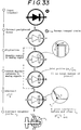
- a diode of Fig.33 will be explained in short.
- the figure of diode is read in by an image scanner. This is an optical input or readin of logomarks or illustrations.
- the peripheral lines are extracted.
- the second figure of Fig.33 exhibits the assembly of peripheral lines of the diode. Five peripheral point groups are included in the figure. The upper righthand circles have two concircle peripheral lines.
- the diode has two inner, upper and lower peripheral lines and one outer peripheral line. All the peripheral point groups are designated by two-dimensional coordinate (X,Y).
- the variables X and Y are represented by an intermediate variable t as X(t) and Y(t).
- peripheral lines are integrally approximated by piecewise polynomials defined at the full region of the point groups. Namely, the definition region of the approximation function is equal to the full length of the peripheral closed loop.
- the approximation by the polynomials converts the point series into two continual functions X(t) and Y(t) of t.
- the peripheral lines expressed by X(t) and Y(t) are twice-differentiated at all points with t in order to obtain the curvature at the point.
- the peripheral lines which have a constant curvature at all points are eliminated as a true, integrated circle. The righthand small round is removed in this example.
- Three peripheral point groups remain. Then joints which have a curvature bigger than the determined value are abstracted for the remainder. Some joints are shown by " ⁇ " in the fourth figure of Fig.33.
- This invention enables a set of a computer, image scanner and printer to input original character font, illustrations, logomarks and compress into a small amount of data, memorizes the shortened data and reproduce a copy of the original object in any size with a high quality in a short time.
- this invention similarly allows a computer, image scanner and printer to input original figures, compress two-dimensional data into a small amount of digital data, and memorize the compressed data in a memory device. There is no need to keep the original paper on which the original figures are drawn.
- This invention can realize a paperless storage of illustrations or drawings for the first time.
- this invention succeeds in enhancing the quality of the reproduced figures, because straight lines in figures are extracted clearly as straight lines, circles in figures are extracted as geometrically-regular circles specified by a radius and a center, arcs in figures are also extracted as geometrically-regular arcs defined by a radius, a center and a center angle. Free curves are approximated by linear combinations of Fluency functions.
- Fig.51 and Fig.52 exhibit examples of enlargement and reduction.
- Optical enlargement by a copy machine is likely to invite noise and blur peripheral lines.
- this invention enlarges or reduces figures by mathematical calculations.
- An arc or circle can be reproduced as a mathematically-regular arc or circle in an enlarged scale or reduced scale.
- enlarged figures are clear-cut and definite. Neither peripheral lines blur nor straight lines become wavy.
- the quality of the enlarged figures of the invention excels in comparison with the optically enlarged figures by a photocopy machine.
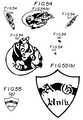
- Fig.53 and Fig.54 are examples demonstrating the freedom of rotation, anisotropic transformation, enlargement and reduction.
- Fig.54(a) enlarges vertically the original figure.
- Fig.(c) slantingly transforms the figure.
- Fig. 54(d) rotates the figure by 90 degrees.
- Fig.54(e) and Fig.54(f) are examples of simultaneous rotation, transformation and reduction.
- Fig. 55 demonstrates examples of enlarging and reducing of the same mark. The position of printing is also freely chosen. These examples are rich in free curves. This invention can be applied even such examples and can find joints in the figures.
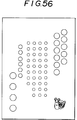
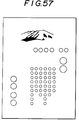
- Fig.56 and Fig.57 show post cards printed with illustrations.
- the post card can be made by enlarging or reducing an original drawing to an arbitrary size and printing the marks at an arbitrary position.
- This invention easily satisfies the requirement.
- Conventionally such a post card has been made by photocopying an original figure to a pertinent size , cutting the copy, and gluing the cut copy at a suitable position of a sheet of paper. This invention saves such tedious manual operations.
- this invention stores the data of figures as joints and coefficients of piecewise polynomials.
- mathematical calculation can enlarge, reduce, transfer, rotate and anisotropically deform the read-in figures. Neither inclusion of noise nor degradation accompanies the operations.
- this invention succeeds in raising the quality of figures by the elimination of redundant joints.
- the transference is accomplished by the parallel displacement of the coordinates of all joints.
- the enlargement and reduction are done by multiplying the coordinates, the radiuses of arcs, the coefficients of piecewise polynomials. A small amount of data facilitates the calculation.
- the rotation demonstrated in Fig.54 can be done only by the calculation of multiplying the coordinates ⁇ (x i (u) , y i (u) ) ⁇ of joints and the coefficients ⁇ c h (x) ⁇ , ⁇ c h (y) ⁇ of approximation functions by the factors determined by the rotation angle.
- the anisotropic enlargement or reduction is done by multiplying different factors to x-components and y-components of the joints or coefficients.
- Fig.1 is a schematic view of apparatus for inputting and outputting of character font, logomarks and illustrations of this invention.
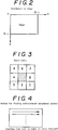
- Fig.2 is a view of coordinates defining pixels on an image on which a character, logomark or illustrate is input.
- Fig.3 is a view of chain codes defined around a pixel.
- Fig.4 is a figure showing the way of finding peripheral points in an image data.
- Fig.5 is a figure showing the way of finding another peripheral point when a peripheral point has already found.
- Fig.6 is a figure demonstrating the current peripheral point and the succeeding peripheral point in the region in which white pixels and black pixels exist.
- Fig.7 is figures showing the process of abstracting an outer peripheral line and an inner peripheral line and assigning value "2" to the pixels .
- Fig.8. is a flow chart showing the function of the peripheral line extracting device.
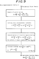
- Fig.9 is a flow chart of the function of the data approximation device for approximating peripheral point groups.
- Fig.10 is a flow chart of the process of determining the coefficients for approximating the whole of the peripheral point groups.
- Fig.11 is a flow chart for calculating the curvature at all points on the peripheral line.
- Fig.12 is a flow chart of abstracting integral circles from the peripheral lines.
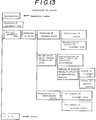
- Fig. 13 is a flow chart of processes for extracting joints.
- Fig. 14 is a flow chart of abstracting joints from the curvature calculated.
- Fig.15 is figures of original mother characters of " " and " "for making a character font.
- Fig. 16 is figures of peripheral lines of " “ and “ “ on which joints are denoted by ⁇ .
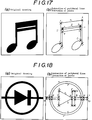
- Fig.17 is figures of sixteenth note as an example of logomarks.
- (a) is an original draft.
- (b) is the peripheral lines on which joints are denoted by ⁇ .
- Fig. 18 is figures of a diode as an example of logomarks or illustrations of diode. (a) is an original figure and (b) is peripheral lines having joints.
- Fig. 19 is a flow chart for extracting optimum joints.
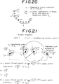
- Fig.20 is a figure for defining the numbers of a temporary joint and neighbouring joint candidates.
- Fig.21 is a figure for clarifying the definition of numbers of temporary joints and output neighbour joints.
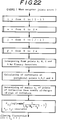
- Fig.22 is a flow chart of the decision of matching coefficients when neighbour joints exist.
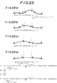
- Fig.23 is figures demonstrating the curve connecting A, B, C and D and the numbers of the turning points in the curve, where C is a joint candidate near a temporary joint selected by the bigness of curvature, B is a joint candidate of output neighbour, D is the next joint of the temporary joint, and A is the joint just before the output neighbour joint candidate B.
- Fig.24 is a flow chart for determining matching coefficients when no neighbouring joint exists.
- Fig.25 is a figure for explaining the definition and numbers of the joint candidate B of the temporary joint, forward joint candidate A for another temporary joint and backward joint candidate C for the other temporary joint when the temporary joint has no neighbouring joint.
- Fig.26 is a figure for demonstrating the definition and numbers of the joint candidate C near the temporary joint selected by the bigness of curvature, another joint candidate B near a neighbouring joint of input neighbor and another joint candidate D of a temporary joint just before the temporary joint.
- Fig.27 is a flow chart for determining whether neighbouring joints are input neighbour or output neighbor.
- Fig.28 is a flow chart showing the definition of the probability variables and the repetition of calculation of the probability variables which estimate the matching of the joint candidate.
- Fig.29 is a flow chart showing another way of determining the matching coefficients.
- Fig.30 is an explanatory figure exhibiting initial probabilities given to 2 ⁇ +1 joint candidates in the vicinity of a temporary joint.
- Fig.31 is a figure for demonstrating the steps of calculating probability variables of all temporary joints, assigning the joint candidate which gives the biggest probability to the optimum joint and memorizing the optimum joint.
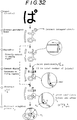
- Fig.32 is an explanatory figure for retrospecting the processes mentioned in short by an example of " (pa)".
- Fig.33 is an explanatory figure for retrospecting the processes mentioned in brief by an illustration of a diode.
- Fig.34 is a flow chart for eliminating unnecessary joints and for determining optimum joints.
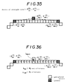
- Fig.35 is a figure of pixels for showing end joints and an intermediate joint which is now judged whether to be eliminated or not, when plural joints of straight line align in series.
- Fig.36 is an explanatory figure denoting the elimination of the intermediate point, when the vertical line drawn from the intermediate joint is shorter than a threshold.
- Fig.37 is a figure for showing end joints and intermediate joint of circle which is now judged whether to be removed or not, when more than three joints lie along a circle.
- Fig.38 is a figure showing the radius and center of the circle beginning from the first joint, and the radius and center of the circle beginning from the second joint.
- Fig.39 is a flow chart for explaining the processes of inputting peripheral point groups, final joints and integral circles, approximating the data, and expressing the peripheral points by approximation functions.
- Fig.40 is figures of (a) an original character " (tai)" to be compressed and stored in a memory and (b) a character “ (tai)” reproduced from the stored data according to this invention.
- Fig.41 is figures of (a) an original character " (go)" to be compressed and stored in a memory and (b) a character “ (go)” reproduced from the stored data according to this invention.
- Fig.42 is figures of (a) an original character " (mei)" to be compressed and stored in a memory and (b) a character “ (mei)” reproduced from the stored data according to this invention.
- Fig.43 is figures of (a) an original illustration of a sixteenth note to be compressed and stored in a memory and (b) a final illustration of a sixteen note reproduced from the stored data according to this invention.
- Fig.44 is figures of (a) an original illustration of a circular graph to be compressed and stored in a memory and (b) a final illustration of a circular graph reproduced from the stored data according to this invention.
- Fig.45 is figures of (a) an original illustration of a tobacco to be compressed and stored in a memory and (b) a final illustration of a tobacco reproduced from the stored data according to this invention.
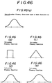
- Fig.46 is figures of a second order fluency function, 0-th order fluency function, first order fluency function and third order fluency function.
- Fig.47 is figures of approximating arbitrary data by Fluency functions as base functions and of showing an arbitrary function which can be precisely approximated by heightening the dimension of the Fluency functions.
- Fig.48 is figures demonstrating the processes for approximating all the peripheral point groups by piecewise polynomials by quoting the Chinese character " (wa)" as an example.
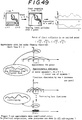
- Fig.49 is figures demonstrating the processes for approximating all the peripheral point groups by piecewise polynomials by quoting an illustration of tobacco as an example.
- Fig.50 is figures of (a) an original drawing of a diode to be compressed and memorizes by this invention and (b) a drawing reproduced by the memorized data.
- Fig.51 is an example of a logo-illustration with many free curves.
- Fig.52. is a reduced figure of Fig.51 which has been compressed, memorized and reproduced in a reduced size.
- Fig.53 is an example of a logo-illustration including many free curves.
- Fig.54 is figures which are reproduced by compressing the illustration of Fig.53, memorizing the data, and reproduced from the data with anisotropic reduction or rotation.
- Fig.55 is an example including modified characters and logomarks. (a) is a reduced figure and (b) is an enlarged figure. One can be transformed to the other by this invention.
- Fig.56 is an example of a mail card in which an illustration of a snail has been interposed by this invention.
- the position or size can be arbitrarily selected.
- Fig.57 is an example of a mail card in which an illustration of a mountain has been inserted by this invention.
- Character font, logomarks or illustrations written on paper are read in by an optical means.
- the read-in data are input as two-dimensional data into the first image memory. If the original object is monochromatic one, lines, dots or other written parts become black pixels in an image screen. The other parts of blank become white pixels. A pixel takes only two value, i.e. black or white.
- the original characters, logomarks or illustrations may be colored. But the image memory stores the object with only two-value data to each pixel. A pixel is also assigned either to white or black in the colored object. The colored parts become black and the rest parts which do not construct the characters, logomarks or illustrations become white. The data of black or white are memorized to all individual pixels.
- the object is input by an image scanner with a precision of 256 dots ⁇ 256 dots.
- the number of dots of input is arbitrarily selected. Bigger number of dots in the image scanning will enhance the quality of the input image. However, if the number of dots ( number of pixels) is large, it will take much time and have much memory capacity to calculate or store data. Thus, a pertinent size of an image scanner shall be chosen.
- the image data of the object are discriminated dot by dot whether the datum is black or white and stored to a memory pixel by pixel in the image memory.
- the dot in an image screen is sometimes called a pixel.
- the word "pixel" is entirely equivalent to a dot.
- a sequence of black pixels is called a point series or a point group.
- a point means a black pixel.
- a dot may be a white pixel or black pixel.
- the position of a point is designated by a coordinate (X,Y), where X is the column number of counted pixels from the top to the bottom in the vertical direction and Y is the line number of counted pixels from the left to the right in the horizontal direction.
- the coordinate variables will be discriminated by affixing various suffixes.
- the peripheral point extracting device extracts the peripheral lines of the characters, logomarks or illustrations read into the image memory.
- the operation of extraction is done by the steps of:
- Peripheral point series is a series of continual black dots enclosing an assembly of black dots.
- a peripheral point series exists in the inner blank of an annular, closed assembly of black pixels as well as on the outer periphery.
- a closed set of continuous peripheral points is called "peripheral point series”.
- U denotes the total number of peripheral point series.
- U series of peripheral points are designated by numbers from 0 to U-1.
- u is the number of the series of peripheral points.
- Series number "u” takes an arbitrary value between 0 and U-1.
- the total number of peripheral points contained in the series u is designated by N(u).
- "k” is the number of a peripheral point in the series u. Point number "k” is an integer between 0 and N(u)-1.
- Chain codes are the numbers from 0 to 7 allocated to eight neighboring pixels around a pixel clockwise. The chain codes will be used to signify the continuity of peripheral points as well as to investigate the continuity of the points. "c" denotes a chain code.
- Peripheral lines are extracted from the image data on the basis of the functions defined so far.
- a black pixel is discovered by scanning the whole image from uppermost dot to the lowest right dot.
- Fig.5 shows the order of tracing for peripheral points.
- the tracing front has found a peripheral point of a peripheral point series.
- eight neighbor pixels around the last-found peripheral point are investigated clockwise whether the pixels are black or white.
- Fig.6 demonstrates the search of the next peripheral point.
- the point marked by " " is the last-found peripheral point.
- the search of Fig.4 shall be started again in order to a next peripheral point. If the next point is found, the peripheral point series to which the found peripheral point belongs will be searched in the similar manner.
- the object character, illustration, drawing, logomark or logotype
- the same procedure will be repeated from the uppermost line to the lowest line in order to discover and determine all point series.
- the series of peripheral points are assigned with the numbers 0,1,2, ⁇ ,and (U-1).
- the object has an inner hole as shown in Fig.5, several times of searches find out a peripheral point belonging to the inner peripheral point series.
- the following points will be similarly searched by the way of Fig.6.
- the points will be traced counterclockwise (Fig.5).
- all peripheral points will be searched in the similar way.
- the coordinates of all the points will be memorized in a memory.
- Fig.7 demonstrates the example.
- (a) is an annular pattern with one pixel width.
- Fig.7(c) shows the result.
- the rest of the black dots which exist at inner regions by more than two pixel thickness in black patterns are unnecessary to define the patterns. Determination of the peripheral points enables us to define the pattern without ambiguity.
- the coordinates of the inner black dots need not be memorized at all.
- the data of the inner black pixels are erased entirely. The elimination of the data alleviates the load of memory to a great extent.
- the peripheral point memory is a device for storing the parameters defining the peripheral points.
- U is the total number of the series
- u is the number of series.
- N(u) is the total number of the peripheral points of the u-th series.
- k is the number of point of the u-th series.
- (x k (u) ,y k (u) ) means the two-dimensional coordinate of the k-th peripheral point of the u-th series. All peripheral points in the u-th series are represented by assigning values 0,1,2, ⁇ ,N(u) to k. All series are cited by taking values 0,1,2, ⁇ U-1 for u.
- This invention includes two data approximation devices.
- the first device is now explained.
- the first data approximation device is affixed with A to distinguishing the latter one.
- the first approximation is required to determine joints by calculating curvature of the peripheral point series.
- Joints are one of most important concepts of this invention. Joints mainly base this invention. A joint is determined by calculating curvature of the peripheral lines. Without preliminary processing, the curvature may be calculated from discrete point data of peripheral lines directly. This invention can utilize such curvature by the discrete calculation.
- curvature will be calculated by approximating the peripheral point series with piecewise equations and differentiating the peripheral line function twice.
- this invention employs a more sophisticated way.
- "t” is adopted as an independent variable.
- "x” and "y” are dependent variables on t.
- the peripheral points (x,y) are approximated by second order piecewise polynomials of t.
- the degree of approximation is estimated by the method of least squares.
- the approximation shall be renewed by increasing the base functions of piecewise polynomials, if the deviation is still too much. Several repetitions of calculations will bring about a sufficient approximation by piecewise polynomials.
- the approximation aims not to obtain the final result but to calculate curvature for determining joints.
- the coordinate of the k-th point of the u-th series is denoted by (x k (u) ,y k (u) ).
- a set of coordinates of the periphery is obtained from the previously explained peripheral point memory.
- Fig.9 shows the processes for approximation. All coordinates (x k (u) ,y k (u) ) are read in from the peripheral point memory. Two dimensional coordinates is now expressed by an intermediate variable t.
- a set of variables (x k (u) ,y k (u) ) is divided into two sets of independent variable t and dependent variables x and y; (t k (u) ,x k (u) ) and (t k (u) ,y k (u) ).
- the adoption of the intermediate variable t reduces two-dimensional problem to one dimensional problem.
- the second block of Fig.9 demonstrated the division of variables into two sets of variables. The same procedures will be done for both sets of(t k (u) ,x k (u) ) and (t k (u) ,y k (u) ). Thus only the calculation of (t k (u) ,x k (u) ) is explained from now onward.
- S x (t) is a function for approximating the u-th series of peripheral points (t k (u) ,x k (u) ).
- S x (t) is given by the linear combination of a set of second-order fluency functions ⁇ m ⁇ .
- (t k (u) ,y k (u) ) is also approximated by S y (t).
- the method of least squares estimates the degree of matching of the approximation with the original peripheral points. The tolerance for error is predetermined. If the error of the approximation equations from the original coordinates is within the threshold, the approximation is satisfactory for calculating curvature. If the error is still beyond the threshold, the approximation shall be renewed by increasing the number of base fluency functions. The approximation function will be defined on the increased bases.
- S x (t) (also S y (t)) is the linear combination of the fluency base functions.
- S(t) shall be expanded with coefficients on the non-periodic, m-th order Fluency functions ⁇ (t) as bases.
- Fluency functions are functions invented by the inventor(Mr.Toraichi). The name “Fluency” has also been named by the inventor. Fluency has been named after the character of connecting points which are as fluent as possible. Fluency functions differ from spline functions which have been used for approximation. Fluency functions are superior to spline functions in the performance of approximation. "m” is the order of the polynomials. M is the dimension which is the number of pieces divided in the definition region. The definition region is written as [0,T]. A parameter k is suffixed to a Fluency function as ⁇ k (t). C k (x) is a coefficient of the linear combination.
- the symbol "+" affixed the bracket ⁇ means taking only a positive value of the bracket. If value in the bracket is negative, the bracket shall be 0.
- (t-a) m + (t-a) m for t>a 0 for t ⁇ a
- the base function ⁇ k (t) is a one-peak function which has definite (non-zero) values in (m+1) pieces from the k-th piece to the (k+m+1)-th piece.
- the base function ⁇ (t) must be zero.
- T is the full length of definition region of t.
- M is the dimension which is equal to the number of division of the definition region T.
- the one unit of the division (T/M) is called a piece.
- M pieces (T/M) form a definition region T. All the coefficients of the base functions are uniquely defined within the definition region T.
- the length of T can be arbitrarily defined.
- the definition length T may have a common length. Otherwise T has a length in proportion to the number of peripheral points N(u). This invention preliminarily approximates the whole of the series of peripheral points with fluency functions without joints (which will be clarified later).
- Fig.46(a) shows a second order Fluency function as a base. This is a piecewise polynomial. The polynomial is expressed by a quadratic curve ranging within three pieces. The rising at the first piece is quadratic and the falling at the third piece is also quadratic. The peak of the second piece is quadratic, too. The function has different quadratic equations in different pieces. At the boundaries of pieces, the values of the functions themselves and the first order differential coefficient are equal in both pieces.
- the zero-th order Fluency function is a rectangular function which takes a single value only in a piece.
- Fig.46(b) is the zero-th order Fluency function.
- the first order Fluency function is a triangle function which exists in two pieces, as shown by Fig.46(c).
- the third order Fluency function is a smooth cubic function, which spans in four pieces, as shown in Fig.46(e).
- the m-th order Fluency function (m ⁇ 2) is a smooth m-th order function which ranges in (m+1) pieces and has a peak at the middle.
- the function rises in the 1st piece in m-th order and falls in the (m+1)-th piece in m-th order.
- the function is also m-th order at the middle peak.
- the base function ⁇ k (t) is identified by a parameter k. "k" denotes the position of the function. An increase of k by one displaces the same function to the right by one piece.
- every piece has (m+1) base functions ⁇ k (t) substantially, because other base functions are all zero in the piece. It is possible to adopt more than third order (m ⁇ 3) Fluency functions.
- the coefficients (-1) q / ⁇ q!(3-q)! ⁇ are determined by the condition that ⁇ k (t) must vanish in the (k+4)-th piece.
- the number of the base functions is (M + 5).
- Fig.47 will be helpful in understanding.
- Fig.47(a) shows data points for example.
- the definition region of data points is 0 to T.
- the base functions and coefficients are so few that any linear combination of the base functions gives the data a poor approximation.
- an increase of the dimension M improves the approximation.
- any complexity of change can be approximated to a satisfactory extent by enhancing the dimension M.
- the degree of approximation is estimated by the fidelity that S x (t) and S y (t) represent the original peripheral point series (x k (u) ,y k (u) ).
- the method of least square is utilized to estimate the quality of the approximation.
- "Q" designates a sum of the squares of differences between approximating functions S x (t) and S y (t) and original coordinate (x k (u) ,y k (u) ).
- the method of least square demands the minimum of Q.
- the coefficients of the base functions are obtained by minimizing Q.
- the scope of summation is the whole peripheral points belonging to a peripheral point series u.
- Fig. 10 demonstrates a flow chart for the data approximation. Determination of coefficients c h is the purpose of the flow chart.
- the dimension M is a parameter for approximation.
- the coefficients c h are uniquely determined from Eq.(10) for a dimension M. However, the coefficients for the value of M do not necessarily satisfy the requirement imposed by the method of least square. If Q is still bigger than a threshold, the dimension M shall be increased by one for improving approximation. Thus, the dimension is a parameter for signifying the hierarchy of approximation. The calculation is repeated by increasing M by one, till the error Q of the method of least square decreases below the threshold. When the approximation attains a satisfactory degree, the coefficients c h at the value of M are finally ascertained.
- the latter terms c h (x) of the righthand are a (M+5) dimensional column vector.
- a vector of C is denoted by an enlarged character c now.
- the suffix "T" indicates a transposed matrix.
- b x G C x This is a matrix equation for seeking vector C x.
- the coefficients ⁇ c k (u) ⁇ can be obtained by multiplying the reverse matrix G ⁇ 1 of G .
- C x G ⁇ 1 b x
- the coefficients ⁇ C h (x) ⁇ of the present dimension M are determined by the matrix equation. This is the calculation of x-component. Similar calculations are carried out for y-component.
- the initial dimension M is 1.
- Eqs. (23) and (28) determine the coefficients C h (x) and C h (y) of S x (t) and S y (t) which approximate the first peripheral point series (x k (u) ,y k (u) ).
- Fig.48 again demonstrates the processes of approximation of a character font.
- a Chinese character e.g. " " is input to an image memory by an image scanner.
- a scanning front scans the image from the left, uppermost pixel (0,0).
- the first point with which the scanning front meets is designated by (t0 (0) , x0 (0) ) and (t0 (0) , y0 (0) ).
- the coordinates (x,y) of the found points are indicated in series by the intermediate variable t.
- the righthand graph of points exhibits an example of x(t) and y(t).
- the dimension M indicates the degree of approximation.
- Three base functions ⁇ ⁇ 2(t), ⁇ ⁇ 1(t) and ⁇ 0(t) have definite values (non-zero) in the piece.
- a curve shown at the middle figure of Fig.48 is obtained.
- Enlarged curve is shown at the left extension with original points, which indicates large errors of the curve.
- the definition region is divided into two pieces [0, 0.5] and [0.5, 1].
- the base functions increase to four, i.e. ⁇ ⁇ 2(t), ⁇ ⁇ 1(t), ⁇ 0(t) and ⁇ 1 (t). Similar approximation is repeated on the four base functions.
- FIG.49 again explains the approximation in the case of logomarks or illustrations.
- An illustration of tobacco is input by an image scanner on a display and in an image memory.
- a tracing front scans tobacco from the uppermost, left pixel (0,0).
- the tracing front meets for the first time with a point of the figure.
- the point is the initial point.
- the coordinates are represented by (t0 (0) ,x0 (0) ) and (t0 (0) , y0 (0) ).
- the tracing operation starts from the initial point for extracting a peripheral line. Extraction of peripheral points gains two series of peripheral points.
- the curvatures are calculated in succession at all points of all series. If the k-th point has been calculated, the similar treatment is done to the (k+1) point.
- the (u+1)-th series is reckoned.
- This device judges from the data of curvatures whether a peripheral point series form a true, integral circle or not.
- an integral circle is an isolated, complete round with a 360 degree circumference. The completeness of circle is denoted by "integral”. Partial circles with less than 360 degree circumference are distinguished from integral circles. Isolation is another requirement of the integral circle. Even if a circle is complete, the circle which intersects with other lines is not an integral circle.
- This device extracts only integral circles among the peripheral point series. In general, characters, logomarks, illustrations or handwritten drawings include plenty of integral circles. Such integral circles are extracted at first. From the diode of Fig.33, the upper righthand two circles are eliminated by the integral circle extraction device. From the circular graph of Fig.44, the outer circle is removed by the integral circle extraction device. The integral circles are excluded from the succeeding approximation.
- An integral, true circle is defined by the constant curvature at all points. The property allows the device to extract integral circles from other patterns.
- Fig. 12 is a flow chart of the integral circle extracting device.
- all the data of curvatures ⁇ K(t k (u) ) ⁇ are input from the curvature memory.
- the following processes decide whether the present peripheral point series forms a true, integral circle.
- An upper limit ⁇ 1 of curvatures is predetermined. If the average curvature is more than the upper limit, the point series does not form an integral circle.
- the point series has a probability that the point series forms an integral circle.
- the above is the function of the integral circle extraction device.
- An integral circle memory stores the coordinates (X,Y) of the center and the radius r of the integral circles which have been found in the former step. Only three parameters are enough to describe the form of the peripheral point series of an integral circle.
- the original pattern is an isolated circle painted overall with black.
- the original pattern is a round " ⁇ " of, e.g. " , , , , ".
- a joint is defined as a junction point between a straigh line and another straigh line, a junction point between a straight lint and a curve, or a junction point between a curve and another curve.
- Two lines with different inclinations meet each other at the junction point.
- the junction point is simply called a joint.
- the joint can be deemed as a point at which a line changes the inclination discontinuously.
- joints are totally a new concept discovered by the Inventor, it is important to clarify the definition, role, significance, and abstraction of joints. Precise, pertinent determination of joints enables this invention to maintain the data of, e.g. character font, logomarks and illustrations at high quality and to minimize the quantity of the data. Joints effectively compress the data of objects, keeping the quality at a high level.
- Fig.13 demonstrates the processes for extracting points.
- An object e.g. character, logomark, illustration or drawing is input by an image scanner into an image memory and on a display at first.
- An image of the object is digitalized into a binary image which includes only white (blank) pixels and black pixels.
- Peripheral point series are extracted from the binary image.
- Joints are extracted from the peripheral point series by the following processes. First clear-cut joints are extracted. The joints are determined by a large curvature. The clear-cut peripheral joints are not optimum but still temporary. Thus, the clear-cut joints are called temporary joints. However, the temporary joints determined from the bigness of curvature are still insufficient for obtaining all necessary joints. On the contrary, unnecessary joints may be included in the temporary joints.
- the determination of joints requires a revision.
- the joints at a right angle part are extracted after the temporary joints have been found.
- the extraction of the joints of a right angle part is important to smooth the junctions at crossing points of lines in the object, e.g. character, logomark, drawing or illustration.
- the joints of straight lines are extracted in addition to the temporary joints.
- the joints of straight lines are abstracted by the bigness of curvature in the case of broad straight lines.
- an initial point or final point cannot be abstracted by the condition of the greatness of curvature.
- Such addition of joints is hardly required to treat characters, because all lines have some broadness.
- illustrations , figures or logomarks often require the addition of the joints of straigh lines, because they often include very thin lines with a width as small as a pixel.
- the temporary joints sometimes include unnecessary joints. Such joints must be removed for heightening the quality of reproduced patterns as well as reducing the quantity of data.
- One kind of needless joints is the joints contained in straight lines. Sometimes a temporary joint lies midway in a straight line with a very small distance from the straight line. If removal of the midway joint does not impair the straightness of the lines, the temporary joint shall be removed, because the joint has been produced by noise.
- the other kind of needless joints is joints included in arcs (partial circles). Occasionally a redundant temporary joint lying midway in an arc splits the arc which has been inherently a single arc into two partial arcs. Such a midway joint should be removed. The removal of the redundant joint redounds to an unification of two arcs into a single arc.
- the lines connecting neighboring joints shall be approximated by piecewise polynomials.
- a line by a pair of neighboring joints is called a definition region.
- the peripheral closed loop changes the inclination drastically at the joints, because a big curvature is equivalent to a big change of inclination of the line. But inclination is constant or changes smoothly in the intermediate part between two neighboring joints, i.e. a definition region.
- the line (or curve) of a definition region can be approximated by a straight line, an arc or a set of polynomials.
- the approximation of peripheral points is similar to the previous approximation described at [D.
- First temporary joints are abstracted from the data of peripheral point series.
- joint has a big curvature from the definition.
- the inclination of the curve changes distinctly at a joint.
- Joints are important points which determine the definition region of approximating functions. Lines between neighboring joints are either straight lines or smooth curves in which the inclination changes continuously. In any cases, the lines between two neighboring joints can be expressed with simple approximating functions, if the selection of joints is suitable. All necessary data are established by calculating all approximation functions representing all the definition regions.
- the points with a curvature bigger than ⁇ are assigned to temporary joints.
- the coordinates (x k (u) ,y k (u) ) of the joints are stored in a joint position memory I. "i" denotes the number of temporary joints hereafter.
- the i-th temporary joint is indicated as d i (x i (u) ,y i (u) ).
- the parameter k of peripheral points is replaced by the new parameter i.
- parameters k and i are affixed to coordinates x and y, k indicates peripheral points and i designates joints selected from peripheral points.
- the comparison of K(t k (u) ) with ⁇ is carried out at all peripheral points of the u-th series. Then the similar procedures are repeated to the (u+1)-th series. Thus all coordinates of temporary joints of all peripheral point series are extracted.
- Fig. 15 shows mother characters of " " (a) and " "(b). The characters are input into an image memory. The peripheral points are extracted. The joints are extracted from the peripheral points. Fig.16 shows the result of the extraction of joints. Symbols " ⁇ " indicate joints.
- Fig.17 is an example of a musical note (sixteenth note).
- the note contains two vertical lines on right and left sides and two slanting lines connecting the two vertical lines. Ellipsoids hang at the feet of the vertical lines.
- Fig.17(a) is an original figure.
- Fig.17(b) is the result of the peripheral point extraction and the joint extraction.
- the points with " ⁇ " are joints.
- the figure has only two peripheral lines ⁇ and ⁇ .
- Peripheral line ⁇ is an outer longer peripheral loop.
- Peripheral line ⁇ is an inner shorter loop.
- the outer peripheral loop ⁇ has joints ⁇ , ⁇ , ⁇ , ⁇ , ⁇ , ⁇ , and ⁇ .
- Line ⁇ - ⁇ , line ⁇ - ⁇ , line ⁇ - ⁇ , line ⁇ - ⁇ , line ⁇ - ⁇ , line ⁇ - , and line ⁇ - ⁇ are straight lines.
- Line ⁇ - ⁇ and line - ⁇ are free curves.
- the inner loop ⁇ has straight lines ⁇ - ⁇ and ⁇ - ⁇ .
- Other lines ⁇ - ⁇ and ⁇ - ⁇ are arcs or free curves. This example has many straight lines. It is important to specify a straight line in the figure as a straight line in the compressed data.
- Fig. 18 is an example of a diode.
- Fig.18(a) is an original figure which has a large circle, a small triangle, a short vertical line, and a long horizontal line.
- Fig. 18(b) shows the result of the extraction of peripheral lines and extraction of joints.
- the figure contains three peripheral point series: an outer circular peripheral line ⁇ and two inner peripheral lines ⁇ and ⁇ .
- the outer peripheral line has eight joints. Symbols ⁇ , , ⁇ , ⁇ , ⁇ and H are attached only to upper-half joints.
- Line ⁇ - is a short straight line.
- Curve - ⁇ is a half circle.
- Line ⁇ - ⁇ is a short straight line.
- Line ⁇ -H is a short straight line.
- Line ⁇ - ⁇ is a free curve.
- Line ⁇ - ⁇ is a straight line.
- Line ⁇ -A is a straight line.
- Line A-B seems a straight line, but is truly a free curve, because it turns a little near B.
- Line B- ⁇ , line ⁇ - ⁇ , line ⁇ -E and line E-Z are straight lines.
- Line Z- ⁇ is a half circle. The figure is also constructed mainly by straight lines. The majority of lines are straight lines. Next majority are arcs. Few lines are free curves.
- Geometry defines such a part of a straight line having both ends as a segment of a line, a half part having one end as a half line and a full straight line with no ends as a straight line.
- this specification calls a segment, a half line and a full line of a straight line as a straight line for simplicity.
- the proportion of straight lines, arcs and free curves depends on the original objects.
- Japanese cursive characters, e.g. " ", " "” include many free curves.
- Chinese characters contain many straight lines.
- Drawings, marks, and illustrations include various proportions of straigh lines, arcs and free curves.
- Three kinds of lines, i.e. a straight line, an arc and a free curve are fundamental elements.
- the diode of Fig.18 has many straight lines. But all marks or drawings do not necessarily include straight lines as the majority. Some of drawings include many arcs (e.g. Fig.45 and Fig.56). Others mainly include free curves (e.g. Fig.51, Fig.53, Fig.55 and Fig.57). Drawings, illustrations or logomarks are produced by designers from free passions. No body knows the proportion of the fundamental elements included in the drawings.
- Joint position memory memorizes the numbers and the coordinates of the temporary joints obtained by the former process.
- joints There are different kinds of joints, i.e. temporary joints determined from the bigness of curvature, joint candidates, optimum joints, neighboring joints and final joints which shall be explained later.
- the joints which have been described are temporary joints which have been determined by the greatness of curvature.
- the temporary joints are not necessarily optimum joints.
- noise is frequently included in a readin image stored in an image memory by the reflection, diffraction or scattering of light from the object at lenses or glasses and the invasion of external light.
- the noise sometimes reduces curvatures at junction points of two lines or curves. Owing to the reduction of the curvature, the point which has a big curvature more than ⁇ inherently fails in being extracted as a joint.
- optimum joints must be searched out.
- An optimum joint must lie in the vicinity of the temporary joint previously found.
- Optimum joints should be turning points of lines from the definition.
- the optimum joints are inherent to the original object, i.e. character, drawing, illustration or mark.
- Optically-induced noise forbids to determine optimum joints only from the greatness of curvature of the optically-input image without ambiguity.
- Fig. 19 is a flow chart of an optimum joint extraction device.
- u is the number of peripheral point series.
- i is the number of temporary joint in the u-th series.
- I is the total number of temporary joints in the u-th series.
- Joint candidates are introduced to the peripheral points in the vicinity of a temporary joint.
- a joint candidate is a point on the peripheral line distanced by less than ⁇ from the temporary joint.
- a joint candidate of the i-th temporary joint (x i , y i ) is indicated by ⁇ o (i) or ⁇ o (i) (x io ,y io ) accompanied by its coordinates.
- the temporary joint has the suffix of series number u.
- the joint candidate ⁇ o (i) is of course one of the joint candidates near the i-th temporary joint of the u-th series.
- the series number u is omitted from the representation of joint candidate ⁇ o (i) for simplicity.
- One temporary joint has several candidates. 2 ⁇ denotes the number of candidates.
- Suffix "o" is the number of candidates for distinguishing the joint candidate from others (2 ⁇ -1). Joints candidates are defined as ⁇ neighboring peripheral points in front of the temporary joint and ⁇ neighboring peripheral points at the back of the temporary joint as shown in Fig.20. A black dot is the central temporary joint which is denoted as x i (y i is omitted in the representation for the sake of simplicity).
- the position of the temporary joint should be denoted by d i . But instead of d i , x i is used for clarifying the position coordination of the temporary joint.
- the total number of joint candidate O is 2 ⁇ +1.
- An optimum joint is one of the joint candidates. The selection of optimum joints from joints candidates improves the quality of reproduced objects. ⁇ determines the scope of searching optimum joint.
- Neighboring joint is also a new concept indispensable for the construction of this invention.
- the neighboring joint is required for searching optimum joints. "neighbor" means that the point is neighboring to the temporary joint x i on process.
- the definition of a neighboring joint is a temporary joint which lies within a distance ⁇ from the outstanding (present) temporary joint x i and is either connected by a continual peripheral line to the outstanding (present) temporary joint or enclosed by the peripheral loop including the present temporary joint x i .
- the neighboring joint is connected with the outstanding temporary joint on process and is included in a circle of a radius ⁇ having the temporary joint as the center.
- Fig.32 shows an example of the neighboring joints.
- the bottom figure demonstrates the neighboring joints of the present temporary joint x i .
- a small circle of a radius ⁇ is depicted.
- the circle encloses seven other temporary joints.
- Six of the seven temporary joints are connected with the central present temporary joint x i by the continual peripheral lines.
- the six temporary joints are the neighboring joints of x i .
- Another temporary joint in the inner peripheral loop also exists in the circle.
- the inner temporary joint is not directly connected with the temporary joint x i .
- the seven temporary joints are all neighboring joints of x i .
- Fig.33 exhibits another example of neighboring joints in the figure of diode.
- the bottom partial figure has a circle of a radius ⁇ with the center x i .
- the circle encloses five temporary joints.
- Two right temporary joints are clearly neighboring joints of x i , because the two are connected with x i by the peripheral line.
- Lower temporary joint ⁇ is a neighboring joint of x i from the same reason.
- Left lower temporary joint M is not connected with x i . But M is enclosed by the outer peripheral line to which x i belongs. Thus M is also a neighboring joint of x i .
- Left temporary joint N is not directly connected with x i . But it is enclosed by the outer periphery on which x i lies.
- N is a neighboring joint of x i . All temporary joints encircled are neighboring joints of x i in this example.
- j is the number of identifying neighboring joint. Since the temporary joint has been specified by i, the neighboring joint is indicated by j in order to avoid confusion.
- the first condition that the neighboring joint lies within a circle of a radius ⁇ with a center x i is expressed by ⁇ (x i -x j )2 + (y i -y j )2 ⁇ 1 ⁇ 2 ⁇ ⁇
- the other one condition is that the neighboring joint is connected directly with the outstanding temporary joint on process. The reason why the neighboring joint must be connected with the outstanding temporary joint is because the extraction of optimum joints has a purpose of joining a pair of joints at both sides of a crossing point as smooth as possible.
- the neighboring joint should be indicated as d j (x j (u) , y j (U) ) rigorously. But the neighboring joint will be denoted simply by x j . "x j " includes also y-coordinate of course.
- the first case of J ⁇ 1 is further divided into two cases. Outer peripheral points have been traced clockwise. Inner peripheral points have been traced counterclockwise. Some neighboring joints precede the outstanding temporary joint x i . Such preceding neighboring joints are named output neighbor. The other neighboring joints succeed the outstanding joint x i . Such succeeding neighboring joints are named input neighbor. Neighboring joints appear at a crossing point in general. Thus, neighboring joints lie nearly along an extension of a tangent line of the peripheral line at the the outstanding temporary joint x i . Then tangent lines at x i of the periphery are drawn like an arrow toward the direction of tracing.
- the neighboring joint which lies at the top of the arrow is an input neighbor, because the arrow seems to enter the neighboring joint.
- the other neighboring joint which lies at the end of the arrow is an output neighbor, because the arrow seems to emanate from the neighboring joint.
- the definition of input neighbor and output neighbor is rather difficult to understand. Optimum joints shall be selected from joint candidates.
- Fig.21 shows the case of J ⁇ 1 and output neighbor.
- a line which connects four joint candidates is selected from each group of candidates. The line must been a part of a smooth line. Thus, the joint candidates must be chosen in order to maintain the line as smooth as possible. The requirement of smooth connecting line determines the most favorable selection of joint candidates.
- the selected candidates are now called optimum joints. The selection of optimum joints from the candidates is one of the most difficult parts of this invention. Therefore, the way of selection will be clarified in detail.
- x i (near point C) is an outstanding temporary joint which has been first selected by the bigness of curvature. This point is the center of this process.
- the neighboring joint is x j (near B). This is output neighbor.
- the next temporary joint x i+1 (near D) of the outstanding joint x i (near C) and the former temporary joint x j-1 (near A) of the output neighbor x j (near B) shall be into consideration.
- the temporary joints have (2 ⁇ +1) own joint candidates.
- ⁇ l' (j-1) are joint candidates of x j-1 .
- ⁇ l (j) are candidates of x j .
- ⁇ o (i) are candidates of x i .
- ⁇ o' (i+1) are candidates of x i+1 .
- Upper bracketed suffixes j-i, j, i and i+1 denote the origin of the candidate groups.
- Lower suffixes l', l, o and o' mean the number in the group.
- A is one of the candidates ⁇ l' (j-1) .
- B is one of the candidates ⁇ l (j) .
- C is one of the candidates ⁇ o (i) .
- D is one of the candidates ⁇ o' (i+1) .
- the intermediate candidates C and D are variables of (2 ⁇ +1). Lines connecting the four points A, B, C and D are considered. Since C and D have (2 ⁇ +1) variables, there are (2 ⁇ +1)2 different lines which can connect A, B, C and D. The continual line connecting the four points can be obtained by piecewise approximation based on Fluency functions.
- the decision of B and C depends on the degree of smoothness of the connecting line ABCD.
- the line ABCD must have been a smooth straight line or smooth curve in an original object. B and C which give the most smooth interpolation shall be chosen. Selection of the smoothest line refines the figures and excludes the noise.
- the problem is now how to express the condition of the most perfect smoothness of the line.
- the smoothness is estimated by the number of the points of inflection.
- a point of inflection is a point at which the curvature changes its sign.
- a meandering line has many points of inflection.
- Smooth means small fluctuation of curvature.
- a smooth line maintains the curvature nearly at a constant value in some length.
- Smoother line has less numbers of points of inflection.
- Smooth interpolation is safely displaced by few number of points of inflection.
- the criterion of determining B and C is minimizing the number of points of inflection of the connecting line ABCD.
- the approximation calculation of the connecting line ABCD is repeated by changing the parameters l and o by one with regard to B and C.
- the fitness of the candidates ⁇ l (j) and ⁇ o (i) to points B and C is expressed in a form of a probability function.
- the probability function includes a coefficient r ij (ol) designating the smoothness of the line ABCD.
- the coefficient r ij (ol) is named a fitness coefficient.
- i is the number of the outstanding temporary joint x i
- j is the number of the neighboring joint x j
- o is the number of candidate ⁇ o (i) for C
- l is the number of the candidate ⁇ l (j) for B.
- the fitness coefficient r ij (ol) is defined to be 1 for a sufficiently smooth curve and to be a value less than 1 for an unsmooth (meandering) curve.
- the fitness coefficient can be a parameter for estimating the fitting of the curve ABCD.
- Fig.22 is a flow chart for determining the fitness coefficient r ij (ol) in the case of J ⁇ 1 (there is a neighboring joint).
- the scopes of parameters are defined at first.
- "o" is the number of (2 ⁇ +1) candidates of x i .
- l is the number of the (2 ⁇ +1) joint candidates of x j .
- the following calculation shall be repeated with regard to four parameters i, o, j and l.
- K(t w (u) ) ⁇ S x '(t w (u) )S y ''(t w (u) )-S x ''(t w (u) )S y '(t w (u) ) ⁇ / ⁇ S x '(t w (u) )2 + S y '(t w (u) )2 ⁇ 3/2
- w A, B, C and D.
- Fig.23 exemplifies different curves with different number n o of points of inflection. " ⁇ " indicates a point of inflection.
- the curve of Fig.23(c) is better than Fig.23(a) or Fig.23(b).
- Fig.23(c) is still not the best.
- the curve of Fig.23(d) changes little the curvature. The curve is most smoothest one. Clearly this is the best selection of B and C. B and C are temporarily determined.
- the fitness coefficient r ij (ol) should be defined to be 1 at the best case.
- a simple r ij (ol) 1 / c2(n o -c1) is also available for selecting suitable B and C.
- r ij (ol) must have a bigger value for smaller number n o , because r ij (ol) indicates the degree of fitness of the connecting curve ABCD.
- the fitness coefficient r ij (ol) at this stage has been calculated from the numbers of the points of inflection.
- the fitness coefficients will be repeatedly calculated by changing the end points A and D, because A and D are also renewed in order to enhance the smoothness of the connection line ABCD. The iteration of calculations will be explained later.
- the determination of r ij (ol) in the case of J>1 has been clarified.
- Fig.24 is a flow chart for calculating the fitness coefficient r ij (ol) in the case of J ⁇ 1.
- the outstanding temporal joint x i has no neighboring joint.
- Fig.25 shows an example of the temporary joints and joint candidates.
- the peripheral line has the outstanding temporary joint x i , a preceding temporary joint x i-1 and a succeeding temporary joint x i+1 .
- the temporary joints x i-1 , x i , and x i+1 have 2 ⁇ +1 joint candidates ⁇ l (i-1) , ⁇ o (i) and ⁇ h (i+1) .
- A is one of ⁇ l (i-1) .
- B is one of ⁇ o (i) .
- C is one of ⁇ h (i+1) .
- the purpose is to finding the smoothest curve which connects three points A, B, and C selected from the joint candidate groups.
- Fig. 24 defines the scopes of the parameters.
- i is the number of the temporary joint.
- o is the number of joint candidates of the outstanding temporary joint.
- j is inherently a number of neighboring temporary joint. But in this case there is no neighboring joint.
- the temporary joint x j corresponds to the preceding temporary joint x i-1 .
- j i-1. In the flow chart, this is expressed by from i-1 to i-1.
- a curve ABC is considered.
- Points A and B are variables. Since A is one of ⁇ l (i-1) , A changes according to the parameter "l". Since B is one of ⁇ o (i) , B changes according to the parameter "o". On the contrary, point C is a fixed point. C is the point of maximizing P i+1 (t-1) (h) among the joint candidates ⁇ h (i+1) of the next temporary joint x i+1 . "t-1" means the former time of approximation. Three points A, B and C are connected by a line which is approximated by Fluency functions. Variable points A( ⁇ l (i-1) ) and B( ⁇ o (i) ) are denoted by "o" and "l".
- the smoothness of the line ABC is estimated by a fitness coefficient r ij (ol).
- dimension M is the parameter for controlling the degree of approximation owing to Fluency functions. High dimension can enhance the degree of approximation.
- the approximation is also done by the method of Fig.10. However, it takes little time because there are only three points to be joined in this case. The precision of approximation is enhanced by repeating the similar approximation calculation several times. "t” indicates the time of the approximation calculation.
- the error is estimated by the method of least square by the equation similar to Eq.(16) or Eq.(29). " ⁇ max " is a predetermined threshold of the error of the approximation of the line ABC.
- the approximation calculation shall be repeated on the bases of Fluency functions of M+1 dimensions. Raising dimension M of Fluency functions reduces the error of the approximation. The approximation calculation is repeated till the error becomes less than ⁇ max .
- the final dimension is denoted by M.
- the final error is indicated by ⁇ .
- Fig.21 shows the way of determining the smoothest connection curve in the case of J ⁇ 1 and the neighboring joint x j being an output neighbor. Similar calculation will also be done in the case of J ⁇ 1 and the neighboring joint x j being an input neighbor. But the positions of four points are slightly different.
- Fig.26 demonstrates the nomination of four points in the case of input neighbor.
- a neighboring joint x j lies within a circle of a radius ⁇ with the center x i .
- x j is posterior to x i with regard to the direction of tracing of the peripheral line.
- All four temporary joints x i-1 , x i , x j and x j+1 have (2 ⁇ +1) joint candidates ⁇ o' (i-1) ⁇ , ⁇ o (i) ⁇ , ⁇ l (j) ⁇ and ( ⁇ l' (j+1) ⁇ respectively.
- Four points A, B, C and D are taken from the four groups of joint candidates.
- A is one of ⁇ l' (j+1) (x l' (j+1) ,y l' (j+1) ) which maximizes the probability P j+1 (t-1) (l') at the latest stage of approximation.
- B is one of ⁇ l (j) (x l (j) , y l (j) ).
- C is one of ⁇ o (i) (x o (i) , y o (i) ).
- D is one of ⁇ o' (i-1) (x o' (i-1) , y o' (i-1) ) which maximizes the probability P i-1 (t-1) (o') at the latest approximation.
- Four points A, B, C and D are connected by a line which is determined by Fluency function.
- the connection line ABCD is estimated by the fitness coefficient r ij (ol).
- An outstanding temporary joint x i often has neighboring joints. There are two kinds of neighboring joints. One is an input neighbor. The other is an output neighbor. An arrow which connects the outstanding temporary joint x i with other temporary joint is imaginarily drawn to the direction of the tracing of peripheral line. If the arrow enters the neighboring joint, the joint is an input neighbor. If the arrow emanates from the neighboring joint, the joint is an output neighbor.
- the input and output neighbor is a concept which is difficult to understand.
- a joint often has two kinds of neighboring joints. Two kinds of neighboring joints must be distinguished in order to select better joint candidates for making the connecting line smoother.
- Fig.27 is a flow chart for judging whether a neighboring joint is an input neighbor or an output neighbor.
- "i” is the number of the temporary joint x i which plays a central role in the calculation of determining the smoothest curve connecting four points.
- "j” is the number of probable neighboring joints.
- "o” is the number of joint candidates of x i . The data of all the joint candidates ⁇ o (i) of x i are input.
- "d j (x j (u) ,y j (u) )" is the coordinate of the j-th temporary joint x j .
- the first problem is whether d j is one of neighboring joints of the candidate group ⁇ o (i) ( x o (i) , y o (i) ) of x i . If d j (x j (u) , y j (u) ) is a neighboring joint of ⁇ o (i) , d j must satisfy the following inequality, ⁇ (x o (i) - x j )2 + ( y o (i) - y j )2 ⁇ 1 ⁇ 2 ⁇ ⁇ This is an inequality similar to Eq.(35). Eq.(35) uses the coordinates of temporary joints as it is.
- Eq.(42) replaces the temporary joint x i by its joint candidate ⁇ o (i) . If d j satisfies Eq.(42) for some value of o, d j may be a neighboring joint of x i . Further, it shall be investigated whether d j belongs to the same peripheral point series including ⁇ o (i) . If so, d j is a neighboring joint x j of x i .
- Another vector d j d j+b is nearly a tangent line at d j of the peripheral line.
- the vector djd j+b is also directed toward the direction of the tracing.
- An inner product of vector d i-b d i and vector d j d j+b is calculated. If the inner product is small enough, two vectors meet at a right angle each other. The condition is described by the inequality; vector d i-b d i ⁇ vector d j d j+b ⁇ ⁇
- ⁇ is a small constant. If d j suffices (43), d j is an input neighbor.
- d j is stored in a memory as an input neighbor d j(i) input of x i .
- vector d j-b d j has the direction of tracing near d j .
- the inclination of vector d j-b d j is different from vector d j d j+b , because the inclination changes at the temporary joint d j with a big curvature.
- the condition of output neighbor is described by, vector d i d i+b ⁇ vector d j-b d j ⁇ ⁇ If d j satisfies the inequality, d j is an output neighbor of x i . Then, the date is stored in a memory as ⁇ d j output (i) ⁇ .
- Fig. 27 shows the definition due to inner products of vectors.
- Optimum joints can be obtained from the following calculation of probability on joint candidates.
- Fig.28 is a flow chart of the probability calculation. The calculation takes into account the joint candidates and the input neighboring joint and output neighboring joint; ⁇ o (i) (x o (i) ,y o (i) ), d j input (i), d j output (i) where ⁇ o (i) (x o (i) ,y o (i) ) is joint candidates near the outstanding temporary joint x i , "o" is the number of joint candidates.
- d j input is the coordinate of the neighboring joint of x i of the input neighbor.
- d j output (i) is the coordinate of the neighboring joint of x i of the output neighbor.
- the above data are input in the optimum joint extraction device J at first.
- the calculation of probability is iterated several times.
- the times of iteration are denoted by "t".
- the times of iteration may be increased to five times or reduced to three times.
- Probability variable P i (t) (o) is defined.
- P i (t) (o) is the probability that the o-th joint candidate of x i should be the optimum joint instead of x i at the t-th iteration of calculation.
- the joint candidate which gives the highest probability P i (t) among all the candidates ⁇ o (i) at the final iteration is assigned to an optimum joint.
- initial probability is given by some way which will be explained later. Iteration of probability calculations heightens the probability of the joint candidate which is suitable for the optimum joint and reduces the probability of another joint candidates which are not suitable for the optimum joint.
- the probability is determined as follows.
- Complementary probability Q i (t) (o) is introduced for giving another probability of the 0-th joint candidate at t-th iteration.
- the complementary probability Q i (t) (o) is a sum of the input probability q i input (o) and the output probability q i output (o).
- q i input (o) and q i output (o) change according to the time of iteration. But the time parameter "t" is omitted for simplicity.
- the joint candidate of the output neighboring joint x j shall be selected by the criterion that the candidate realizes the smoothest curve in the temporarily restricted requirement.
- Eq.(51) and Eq.(53) select the joint candidates of the neighboring joints x j 's which produce the smoothest curve connecting four points ABCD in Fig.21 or Fig.26.
- the reason why the contributions from the input neighbor and the output neighbor should be added is that the process aims at searching the optimum point among the candidates of x i which maximizes the smoothness of two crossing curves, one of which passes at the input neighbor and the other of which passes at the output neighbor.
- Eq.(55) is written at the bottom of the square of Fig.28.
- the initial probabilities P i (0) (o) can be given in any ways. Here for example, the candidates nearer to the outstanding temporary joint x i are allotted with a bigger initial probability. This allocation is based on the assumption that the optimum joint may lie in the vicinity of the temporary joint x i and the highest initial probability P i (0) (o) of the temporary joint may facilitate the convergence of the probabilities P i (t) (o).
- Fig.30 clarifies the allotment of the initial probabilities P i (0) (o) to the joint candidates ⁇ o (i) .
- There are ( 2 ⁇ +1 ) joint candidates ⁇ o (i) , where "o" is the number ( o 0 to 2 ⁇ +1 ) of the candidates.
- P' i (o) lowers by 2, being distanced by one candidate from the middle temporary joint x i .
- the preliminary values P' i (o) make the initial probability P i (0) (o) by normalizing themselves.
- the initial probabilities P j (0) (l) for neighboring joints or for other joints are similarly predetermined by the similar formula to Eq.(56).
- q i input (o) max ⁇ r ij (ol) P j (0) (l) ⁇ , where the variable is "l" which is the number of the input neighboring joint.
- This equation chooses the most probable candidate of the input neighboring joint for forming the smoothest curve ABCD.
- the parameters "l” and curves ABCD are of course different from each other for the input probability d i input (o) and the output probability d i output (o), although the same notations are used.
- Q i (0) (o) q i output (o) + q i input (o).
- the complementary probability at the zero time iteration is obtained.
- q i output (o) max ⁇ r ij (ol)P j (1) (l) ⁇
- q i input (o) max ⁇ r ij (ol)P j (1) (l) ⁇ .
- the third time probability P i (3) (o) shall be obtained.
- Fig.31 shows the process for determining the optimum joint.
- the number of temporary joints changes from 0 to I-1.
- P i (4) (o) signifies the probability that the o-th candidate ⁇ o (i) of the temporary joint x i should be an optimum joint in the vicinity of x i .
- Fig.31 demonstrates that the optimum joint is determined to the joint candidate ⁇ o (i) which gives max ⁇ P i (4) (o) ⁇ among all candidates of x i .
- the optimum joint replaces the temporary joint.
- the temporary joint now loses the title of a joint. Therefore, an optimum joint can be determined from the joint candidate in the vicinity of a temporary joint x i . Such a calculation shall be done with all temporary joints.
- This invention seeks temporary joints at first from the curvature, develops the probable joints to joint candidates near the temporary joints and determines optimum joints from the candidates. This is an important feature of this invention.
- the revision is based on the discovery of the Inventor that the temporary joints found from the bigness of curvature are not necessarily the most pertinent joints.
- the condition for the optimum joints has been the least number of points of inflection of the curve connecting four points. Namely, the optimum joints are selected from the purpose for obtaining the smoothest curve connecting four points on both sides of a crossing point.
- Alternative for revising the joints is a method of treating directly the curvature of the curves instead of the number of points of inflection.
- Fig.29 is a flow chart of another method for determining the optimum joints directly from the curvature.
- "J ⁇ 1" is the condition that there are some neighboring joints xj near the temporary joint x i .
- an input neighbor and an output neighbor x j are also considered.
- the latest joint and the next joint of x i or x j are taken into consideration for forming a curve connecting the four points as shown in Fig.21 and Fig.26. Then the maximum curvature of the curve is calculated instead of the number of points of inflection.
- Fig.29 clarifies the definitions of maximum curvatures "K output " and "K input ".
- K input is the maximum curvature of the curve connecting four points ⁇ l' (j-1) , ⁇ l (j) , ⁇ o (i) and ⁇ o' (i+1) in the case of the input neighbor. In the four points, two ends are fixed points.
- ⁇ o' (i+1) is the joint candidate which maximizes the latest probability P i+1 (t-1) (o').
- ⁇ o' (i+1) max P i+ 1 (t-1) (o').
- K output is the maximum curvature of the curve connecting another four points ⁇ l' (j+1) , ⁇ l (j) , ⁇ o (i) and ⁇ o' (i-1) in the case of the output neighbor. Two ends are fixed points.
- ⁇ l' (j+1) max P j +1 (t-1) (l' ).
- ⁇ o' (i-1) max P i-1 (t-1) (o').
- the smoothest curve must have the least value of the maximum curvature. The smaller the maximum curvature of a line is, the smoother the line is.
- the least maximum curvature is desirable for forming the smoothest line.
- the another method of this invention defines the fitness coefficient r ij as the minimum of the sum of the maximum curvatures K input and K output .
- r ij (ol) min ⁇ ( K input + K output ) ⁇ 1, 1 ⁇ where ⁇ is a constant which is nearly equal to the least value of (K input + K output ). "min ⁇ a, b ⁇ " is equal to the smaller member of a and b.
- the second square of Fig.29 shows the definition of the fitness coefficient r ij (ol).
- the newly defined fitness coefficient is larger for a curve of smaller curvature.
- the new r ij (ol) can also estimate the smoothness of a curve.
- Three points ⁇ o+l (i) , ⁇ (i) , ⁇ o-l (i) are connected by a curve using the second order Fluency functions.
- r ij (ol) min ⁇ ( A M + B ⁇ ) ⁇ 1,1 ⁇ , where M is the dimension of the approximation and ⁇ is the error of the method of least square.
- ⁇ o (i) is one of the joint candidates of x i .
- ⁇ o-l (i) and ⁇ o+l (i) are other joint candidates distanced from x l by "l" peripheral points.
- the following process is similar to the former method.
- the joint candidate which has the largest probability P i (4) (o) shall be chosen as an optimum joint of the group to which x i belongs. Such a calculation shall be done with all temporary joints.
- the optimum join memory stores all the optimum joints which have been determined in the former processes.
- "u” is the number of the peripheral point series.
- "i” is the number of the peripheral point in the u-th series.
- "i" has been a number of a temporary joint and
- x i has been a temporary joint ( x i represents y i also) so far.
- the representation x i of an optimum joint must not be confused with the representation xi of a temporary joint.
- the common use of "i” will cause no problem, because one optimum joint corresponds to one optimum joint and the optimum joint either is the temporary joint itself or lies near the temporary joint.
- Fig.32 shows the treatment of a character " ".
- the uppermost drawing is the black character which is input into an image memory A by an image scanner.
- Image processing extracts the peripheral point series.
- the peripheral point series are denoted by the blank character of the second drawing.
- the righthand double circles are extracted in the integral circle extraction process and are memorized in the integral circle memory. The double circles are excluded in the following operations.
- the rest is " " which is exhibited by the third drawing of Fig.32.
- the blank " " has three independent peripheral point series. All peripheral points in a series are connected by a closed loop whose form is approximated by piecewise polynomials based on Fluency functions, e.g. the second order Fluency functions as bases. Then the curvatures are calculated at all points by twice-differentiating the piecewise polynomials representing the closed loop. Temporary joints are extracted as the peripheral point with a big curvature. The righthand encircled drawing exemplifies a temporary joint at a corner. In general, temporary joints appear at turning points of the closed loop. The fourth figure of Fig.32 shows some of the temporary joints " ⁇ " abstracted by the bigness of the curvature.
- a blunt corner e.g. sometimes the lower, righthand corner encircled is not abstracted as a joint.
- a joint shall be added to the blunt corner as shown in the second enlarged drawing of Fig.32.
- the sixth figure of Fig.32 shows the extraction of neighboring joints of the temporary joint x i which is the right blunt corner. The processes have already been explained till the extraction of the neighboring joints.
- the treatments are again retrospected on an example of the illustration of diodes of Fig.33.
- This figure is produced by adding an extra round at upper right of the diode of Fig.18 or Fig.50 for clarifying the treatment of integral circles.
- the original drawing is read-in by an image scanner into an image memory A.
- Peripheral point series are extracted by the image processing.
- the blank figure consisting of peripheral point lines is exhibited by the second drawing of Fig.33.
- Two circles at the upper right are extracted by the integral circle extraction and are stored in the integral circle memory.
- the rest is constructed with a round, a triangle and a segment of a line.
- All point series are outlined by curves which approximate the point series with piecewise polynomials based on Fluency functions.
- the curvatures are calculated by differentiating the piecewise polynimials or directly from the peripheral points.
- a corner of the peripheral line is extracted as a temporary joint as shown in the enlarged, encircled figure of Fig.33.
- Temporary joints are denoted by " ⁇ " in the fourth drawing. Turning points or joining points of segments become temporary joints. Since the temporary joints are abstracted by the bigness of curvature, a blunt corner at which two segments meet at an obtuse angle sometimes fails to be selected as a joint.
- the corner shall be added as a temporary joint.
- all turning points can be selected by the curvature. There is no need to add a joint.
- Peripheral points ⁇ , M and N which lie within the circle of a radius ⁇ with the center x i are extracted as neighboring joints of x i .
- the assembly of the joints sometimes includes needless joints.
- the needless joints are generated by various reasons, e.g. the noise inherently included in the original figures, the noise yielded from the optical input of the figures, etc.
- the needless joints will dissipate the capacity of memory and will degrade the quality of reproduced objects.
- the joint elimination device removes the needless joints which are included in straight lines or arcs. Of course unnecessary joints are also contained in free curves. However, free curve has a probability including various partial lines. It is difficult to distinguish needless joints from necessary joints.
- Fig.34 is a flow chart for the elimination of needless joints.
- "i" is the number of joint in a series.
- "u” is the number of the peripheral point series.
- needless, redundant joints are eliminated from straight lines.
- redundant joints in arcs are removed.
- the leftover joints are called final joints. Neither new joints are added to the final joints nor joints are removed from the final joints.
- the final joints are specified by the number "i'” instead of "i”.
- the final joints are memorized in a final joint memory as ( x i' (u) , y i' (u) ).
- Fig.35 shows an intermediate joint existing midway in a straight line.
- the coordinates of the joints are denoted by (X i4 (B) , Y i4 (B) ).
- the joints are estimated one by one.
- End joints (X ns (B) , Y ns (B) ) and (X ns+2 (B) , Y ns+2 (B) ) are connected by a straight line.
- a vertical line is drawn from the intermediate joints (X ns+1 (B) , Y ns+1 (B) ) to the straight line.
- L ns+1 indicates the length of the vertical line.
- the length of the vertical line is smaller than a predetermined constant K7.
- L ns+1 ⁇ K7 the intermediate joints shall be eliminated.
- Fig. 36 demonstrates the final state of the straight line after the intermediate joints has been removed and the end joints are connected by a straight line.
- Fig.37 shows the case of the joints existing on an arc.
- the joint of the arc is denoted by (X i4 (B) ,Y i4 (B) ).
- i4 is the joint number.
- the coordinate of the centers of ⁇ and P are denoted by (x ns , y ns ) and (x ns+1 , Y ns+1 ). Both arcs ⁇ and P shall be deemed as two parts of a single arc, when the following conditions are satisfied by the radiuses and coordinates of the centers,
- the centers are nearly the same points and the radiuses are nearly the same length, the two arcs ⁇ and P are deemed to be parts of the same arc. In this case, the intermediate joints (X ns+1 (B) , Y ns+1 (B) ) should be removed as an unnecessary joint. If the inequalities (60) and (61) are not satisfied, the intermediate joint is maintained.
- Final joints which have been obtained by the eliminating needless joints are stored into a final joint memory.
- the data approximation device B is a device which approximates the objects by the data, e.g. peripheral point series, final joints, integral circles, etc. This is one of the most important parts of this invention.
- Fig.39 shows the data which are input to the data approximation device B.
- the lines starting from arbitrary joints can be distinguished. If the curvatures at all points are 0, the line is a straight line. If the curvatures at all points are the same definite value, the line is an arc. If the curvatures change in the peripheral point series, the line is a free curve.
- the preliminary classification of the shapes facilitates the determination of the parameters in the approximation calculation.
- x-approximation function s x (t) is a first order function connecting the initial point x1 and the final point x n3 .
- y-approximation function s y (t) is a first order function connecting the initial point y1 and the final point y n3 .
- x-function and y-function are first order functions of t.
- the parameter determining the line is the proportional constant of s x (t) to s y (t).
- this proportional constant need not be memorized, because if the initial point (x1, y1) and the final point (x n3 , y n3 ) are known, a straight line can be drawn between two points. Further, the final point (x n3 , y n3 ) will be given as the starting point at the next joint. Thus, the coordinate of the final point need not be memorized at the joint.
- n arc is the quotient of the central angle divided by 360 degrees.
- n arc is 1/4.
- 2 ⁇ n arc is the central angle of the arc.
- the variable 2 ⁇ t/(T/n arc ) is the central angle of the arc from the beginning point to the current parameter t.
- (C x ,C y ) is the coordinate of the center of the arc.
- a x and B y are constants defining the size of the arc.
- the parameters determining the arc are the coefficients A x , B x , C x , A y , B y , C y and n arc of the functions s x (t) and s y (t). If the definition region has been known as an arc from the beginning of the approximation, such parameters can be uniquely determined by the coordinate of the initial point, the final point the intermediate point and the curvature.
- the definition region which is neither a straight line nor an arc is approximated by a free curve.
- the line is also represented by the intermediate parameter t.
- a peripheral point has two dimensional coordinate (x i3 (u) , y i3 (u) ). But the two dimensional coordinate is decoupled into the intermediate variable representation (t i3 (u) , x i3 (u) ) and (t i3 (u) , y i3 (u) ).
- "k” has been a parameter of peripheral points so far. But “k” is used to signify the number of pieces of a definition region from now. Thus, "i3” denotes the number of the peripheral points instead of "k”.
- the total number of the peripheral points is denoted by "n3".
- the approximation functions s x (t) and s y (t) are developed on the basis of the second order Fluency functions ⁇ k3 . Fluency functions are explained in Fig.46.
- the second order Fluency function has non-zero value only in three pieces.
- the definition region is [0, T].
- the functions s x (t i3 ) and s y (t i3 ) are expressed by linear combination of the second Fluency functions with coefficients c k (x) and c k (y) .
- ⁇ k+q ( k + q ) T/M
- the coefficients c k (x) and c k (y) shall be determined to approximate the peripheral points (x i3 (u) , y i3 (u) ) by s x (t i3 ) and s y (t i3 ).
- the method of least square estimates the error. Minimizing the error by the method of least square gives preferable coefficients.
- 2 - ⁇ i3 1 n3
- the condition for minimizing the error Q gives the following sets of equations.
- the coefficients c k (x) , and c k (y) are obtained by solving the sets of equations.
- the peripheral point series of the original character font, logomarks, illustrations or figures have been separated to straight lines, integral circles, arcs and free curves as elementary lines by the processes mentioned so far.
- the elementary lines have starting points, final points, inclinations, centers and radiuses, etc. as the parameters defining the original objects.
- the elementary lines have different kinds of data to be stored.
- a flag which denotes the straight line and the coordinate of the starting point shall be stored.
- the coordinate of the final point is not stored at the stage, because the final point will be given as a starting point of the next definition region.
- the inclination of the straight line which is an important parameter is not also stored because the inclination will become clear by connecting the initial point and the next point.
- the data can be obtained directly from the integral circle memory G.
- the data have been extracted by the first data approximation device A.
- the parameters of an integral circle are a flag indicating an integral circle, a coordinate of the initial point of arc, a ratio of arc (length of arc/ full circle length), the number of peripheral points and the coefficients of the functions.
- the data are the dimension M of the base functions, the number of peripheral points, the middle points of the change of the free curve and the coefficients of the functions.
- the compressed data memory memorizes the data of straight lines, integral circles and free curves. The data will be output later at some suitable timing.
- This device compresses the data and stores the compressed data.
- the structures of the data stored in the compressed data memory P are shown in Table 1.
- a straight line connecting two neighboring joints requires one byte for a flag indicating a straight line and two bytes for an initial joint coordinate (x,y).
- a straight line requires three bytes in all.
- An arc connecting two neighboring joints demands one byte for a flag indicating an arc, two bytes for coordinates of an initial points, four bytes for signifying the center angle of the arc, one byte for indicating the number of peripheral points and twelve bytes for designating the coefficients of the approximation functions.
- an arc needs twenty bytes in all.
- a free curve In the case of a free curve, the line demands one byte for the dimension M, one byte for the number of peripheral points, two bytes for signifying the center of the change of peripheral points and 2M bytes for the coefficients of the approximation function. Therefore, a free curve needs 4+2M bytes in all.
- the periphery reproduction device R, the character ⁇ logomark ⁇ illustration reproduction device S and the reproduced data output device T construct together a reproduced data generation device which can reproduce any original objects into any sizes of reproduced ones.
- Table 1 Data structure produced by this invention Contents size (Byte) Line between joints is a straight line 1. A flag denoting a straight line 1 per line 1. A coordinate of an initial point 2 per line Line between joints is an arc 1. A flag denoting an arc 1 per line 1. A coordinate of an initial point 2 per line 1. A ratio n arc of arc to full circle ( 1/4 ⁇ n arc ⁇ 1) 4 per line 1. Number of peripheral points 1 per line 1. Coefficients of approximating functions ( six ) 12 per line Line between joints is a free curve 1.
- the periphery reproduction device reproduces peripheral lines of the character font, logomarks or illustrations from the compressed data stored in the memory.
- the kinds of peripheral lines are straight lines, integral lines, arcs and free curves.
- a straight line is reproduced by connecting the initial point with the joint of the next definition region by a straight line.
- the data of the inclination are unnecessary.
- An integral circle can be reproduced by depicting a circle having the radius and the center output from the memory.
- the coordinates x and y are obtained from S x (t) and S y (t) by changing the intermediate parameter t in the definition region [0, T].
- peripheral lines have been reproduced by the preceding processes.
- the inner parts of the closed peripheral lines are filled with black pixels.
- original characters, logomarks or illustrations are reproduced.
- the outer parts of closed peripheral lines are replaced by black pixels.
- a reversed figure is reproduced.
- a layout editor which can designate the size of the reproduced image from 1 mm square to A4 size can be used.
- There produced image is printed by a laser printer with 300 DPI fineness or a laser printer with 600 DPI fineness. Otherwise, the image can be reproduced by a cutting plotter or laser cutter with 400 DPI fineness.
- the character font, logomarks or illustrations have been memorized in the form of the coefficients of the functions.
- the position of the reproduced image can be arbitrary designated.
- this invention can output the reproduced image with arbitrary size at an arbitrary position on a sheet of paper, plastic cloth, etc.
- Fig.40 to Fig.42 show the original characters of " “, “ “ and “ “, and the reproduced characters by a 300 DPI laser printer according to this invention. The characters have been reproduced with a high fidelity. Furthermore, the music note of Fig.43, the circular graph of Fig.44 and the tobacco of Fig.45 were treated by this invention. The result is shown in Table 3. Table 3. Quantity of data, Compression ratio, Time for compression (logomarks, illustrations) Quantity of Data Compression ratio Compression time ( Byte ) ( % ) ( sec. ) Music Note 135 1.65 12.23 Circular Graph 284 3.47 8.66 Tobacco 264 3.22 8.48 Average of 50 figures 251 3.06 11.06
- Table 2 and Table 3 indicate the quantity of the data compressed ( bytes ), compression ratio (%), and the time ( sec ) for compression.
- the compression rate is defined as the quotient of the compressed data quantity divided by the original image quantity ( nearly 8 kbytes ). The quotient is multiplied by 100 in order to express the compression rate in percent.
- the original figures for example, are read in by an optical image reader ( image scanner ) with a read-in window of 256 pixels ⁇ 256 pixels. In the case, the original image data are about 8 kbytes.
- the quantity of the data is reduced to 300 bytes to 500 bytes in the case of character font or to 100 bytes to 300 bytes in the case of illustrations by the method of this invention.
- the compression rate is 2 % to 6 % in this invention.
- This invention succeeds in extremely reducing the quantity of image data.
- the time for compression is several seconds per one character or one illustration. It is a very short time.
- the compression time is the CPU time including the time for dividing and synthesizing data and the time for converting the compressed data into graphic data.
- This invention is featured by small quantity of stored data and short processing time.
- printing letters can be treated in a very short time by this invention, because most of the printing letters are mainly built by segments of straight lines which are extracted as clear-cut joints at the first stage of operations. The printing letters have few joints which shall be chosen and modified at the later stage of operations.
- the reproduced character font, logomarks and illustrations are stored in the image memory 2 (U) as it is.
- This memory means all devices which memorize the characters, illustrations or logomarks output by a printer.
- a video camera can be utilized for the memory.
- a printed sheet of paper is another type of image memory. This invention can dispense with the image memory U.
Landscapes
- Engineering & Computer Science (AREA)
- Physics & Mathematics (AREA)
- General Physics & Mathematics (AREA)
- Theoretical Computer Science (AREA)
- Multimedia (AREA)
- Image Processing (AREA)
- Controls And Circuits For Display Device (AREA)
- Image Generation (AREA)
Applications Claiming Priority (4)
| Application Number | Priority Date | Filing Date | Title |
|---|---|---|---|
| JP259137/92 | 1992-09-01 | ||
| JP4259137A JP2646475B2 (ja) | 1992-09-01 | 1992-09-01 | 文字デ−タ入力出力装置と入力出力方法 |
| JP269646/92 | 1992-09-11 | ||
| JP4269646A JP2646476B2 (ja) | 1992-09-11 | 1992-09-11 | ロゴ・イラストデ−タ入力出力装置と入力出力方法 |
Publications (2)
| Publication Number | Publication Date |
|---|---|
| EP0586219A2 true EP0586219A2 (de) | 1994-03-09 |
| EP0586219A3 EP0586219A3 (en) | 1994-06-08 |
Family
ID=26543986
Family Applications (1)
| Application Number | Title | Priority Date | Filing Date |
|---|---|---|---|
| EP19930306856 Withdrawn EP0586219A3 (en) | 1992-09-01 | 1993-08-31 | Apparatus and method for image compression |
Country Status (6)
| Country | Link |
|---|---|
| US (1) | US5572605A (de) |
| EP (1) | EP0586219A3 (de) |
| KR (1) | KR0129505B1 (de) |
| CN (1) | CN1033110C (de) |
| AU (1) | AU656090B2 (de) |
| CA (1) | CA2105125C (de) |
Cited By (4)
| Publication number | Priority date | Publication date | Assignee | Title |
|---|---|---|---|---|
| EP0678833A3 (de) * | 1994-04-18 | 1996-03-27 | At & T Corp | Vorrichtung und Verfahren zur Handschriftdekomprimierung zur geschätzten Taktinformation. |
| EP0806742A1 (de) * | 1996-05-08 | 1997-11-12 | Daewoo Electronics Co., Ltd | Adaptive Konturenkodierung |
| EP1118946A4 (de) * | 1998-06-17 | 2007-05-02 | Niigata Seimitsu Co Ltd | Dateninterpolationsverfahren |
| KR100798536B1 (ko) * | 2004-03-03 | 2008-01-28 | 도꾸리쯔교세이호징 가가꾸 기쥬쯔 신꼬 기꼬 | 신호 처리 장치 및 방법과 신호 처리 프로그램 및 그프로그램을 기록한 기록 매체 |
Families Citing this family (17)
| Publication number | Priority date | Publication date | Assignee | Title |
|---|---|---|---|---|
| JPH0816801A (ja) * | 1994-06-30 | 1996-01-19 | Canon Inc | 画像処理方法及び装置 |
| JP3573465B2 (ja) * | 1996-01-22 | 2004-10-06 | 松下電器産業株式会社 | デジタル画像符号化、復号化方法及びそれを用いたデジタル画像符号化、復号化装置 |
| JP3031613B2 (ja) * | 1996-11-12 | 2000-04-10 | 株式会社つくばソフト研究所 | カラー/濃淡画像入力出力装置と入力出力方法 |
| US6401133B1 (en) * | 1998-06-24 | 2002-06-04 | Unisys Corporation | System for high speed continuous file transfer processing of data files |
| JP3172498B2 (ja) * | 1998-10-02 | 2001-06-04 | インターナショナル・ビジネス・マシーンズ・コーポレ−ション | イメージ認識用特徴値抽出方法、およびその装置、イメージ解析プログラムを格納する記憶媒体 |
| US6584237B1 (en) * | 1999-08-23 | 2003-06-24 | Pentax Corporation | Method and apparatus for expanding image data |
| JP3732978B2 (ja) * | 1999-08-23 | 2006-01-11 | ペンタックス株式会社 | 画像圧縮および伸張装置とその方法 |
| JP3709106B2 (ja) * | 1999-09-10 | 2005-10-19 | ペンタックス株式会社 | 画像圧縮および伸張装置 |
| US6820032B2 (en) * | 2001-02-05 | 2004-11-16 | National Instruments Corporation | System and method for scanning a region using conformal mapping |
| JP4053021B2 (ja) * | 2004-05-12 | 2008-02-27 | 三洋電機株式会社 | 画像拡大装置、及びプログラム |
| US7418145B2 (en) * | 2004-06-30 | 2008-08-26 | Matsushita Electric Industrial Co., Ltd. | Compression device and decompression device |
| TWI254234B (en) * | 2004-12-24 | 2006-05-01 | Hon Hai Prec Ind Co Ltd | System and method for auto-judging geometric shape trend of a set of dots on an image |
| CN100377578C (zh) * | 2005-08-02 | 2008-03-26 | 北京北大方正电子有限公司 | 一种电视字幕文字的处理方法 |
| CN104980619B (zh) * | 2014-04-10 | 2018-04-13 | 富士通株式会社 | 图像处理设备和电子装置 |
| US10347016B2 (en) * | 2016-01-12 | 2019-07-09 | Monotype Imaging Inc. | Converting font contour curves |
| US10936792B2 (en) | 2017-12-21 | 2021-03-02 | Monotype Imaging Inc. | Harmonizing font contours |
| CN111063009B (zh) * | 2019-12-18 | 2021-04-06 | 山东山科智能科技有限公司 | 一种汉字书写动画演示方法及装置 |
Family Cites Families (6)
| Publication number | Priority date | Publication date | Assignee | Title |
|---|---|---|---|---|
| JPH0613212B2 (ja) * | 1983-10-03 | 1994-02-23 | 株式会社写研 | 文字画像デ−タの処理方法 |
| GB2147474B (en) * | 1983-10-03 | 1987-05-07 | Shaken Kk | Method of processing character or pictorial image data |
| JP2735197B2 (ja) * | 1987-11-12 | 1998-04-02 | 株式会社東芝 | 図形入力装置 |
| JP2806961B2 (ja) * | 1989-02-22 | 1998-09-30 | 株式会社リコー | 画像符号化方法 |
| US5233671A (en) * | 1989-02-22 | 1993-08-03 | Ricoh Company Ltd. | Image coding method for coding characters using a modified Bezier curve |
| JPH0458378A (ja) * | 1990-06-28 | 1992-02-25 | Mitsubishi Heavy Ind Ltd | ベジエ曲線を分割して展開する方法 |
-
1993
- 1993-08-30 CN CN93117077A patent/CN1033110C/zh not_active Expired - Fee Related
- 1993-08-30 CA CA002105125A patent/CA2105125C/en not_active Expired - Fee Related
- 1993-08-31 EP EP19930306856 patent/EP0586219A3/en not_active Withdrawn
- 1993-08-31 AU AU46008/93A patent/AU656090B2/en not_active Ceased
- 1993-09-01 KR KR1019930017344A patent/KR0129505B1/ko not_active Expired - Fee Related
- 1993-09-01 US US08/114,364 patent/US5572605A/en not_active Expired - Lifetime
Cited By (6)
| Publication number | Priority date | Publication date | Assignee | Title |
|---|---|---|---|---|
| EP0678833A3 (de) * | 1994-04-18 | 1996-03-27 | At & T Corp | Vorrichtung und Verfahren zur Handschriftdekomprimierung zur geschätzten Taktinformation. |
| US5623555A (en) * | 1994-04-18 | 1997-04-22 | Lucent Technologies Inc. | Method and apparatus for handwriting decompression using estimated timing information |
| EP0806742A1 (de) * | 1996-05-08 | 1997-11-12 | Daewoo Electronics Co., Ltd | Adaptive Konturenkodierung |
| US5774596A (en) * | 1996-05-08 | 1998-06-30 | Daewoo Electronics Co., Ltd. | Adaptive contour coding method for encoding a contour image in a video signal |
| EP1118946A4 (de) * | 1998-06-17 | 2007-05-02 | Niigata Seimitsu Co Ltd | Dateninterpolationsverfahren |
| KR100798536B1 (ko) * | 2004-03-03 | 2008-01-28 | 도꾸리쯔교세이호징 가가꾸 기쥬쯔 신꼬 기꼬 | 신호 처리 장치 및 방법과 신호 처리 프로그램 및 그프로그램을 기록한 기록 매체 |
Also Published As
| Publication number | Publication date |
|---|---|
| KR0129505B1 (ko) | 1998-04-15 |
| KR940007735A (ko) | 1994-04-28 |
| CN1033110C (zh) | 1996-10-23 |
| CN1083954A (zh) | 1994-03-16 |
| AU656090B2 (en) | 1995-01-19 |
| EP0586219A3 (en) | 1994-06-08 |
| AU4600893A (en) | 1994-03-24 |
| CA2105125C (en) | 2000-04-18 |
| US5572605A (en) | 1996-11-05 |
| CA2105125A1 (en) | 1994-03-02 |
Similar Documents
| Publication | Publication Date | Title |
|---|---|---|
| EP0586219A2 (de) | Verfahren und Vorrichtung zur Bildkompression | |
| US5664027A (en) | Methods and apparatus for inferring orientation of lines of text | |
| Chu et al. | Halftone QR codes | |
| US6993185B2 (en) | Method of texture-based color document segmentation | |
| US6347156B1 (en) | Device, method and storage medium for recognizing a document image | |
| JP3056905B2 (ja) | 文字認識方法およびテキスト認識システム | |
| US6185341B1 (en) | Image processing using vector data to reduce noise | |
| CN100568263C (zh) | 布局分析设备和布局分析方法 | |
| Laurentini et al. | Identifying and understanding tabular material in compound documents | |
| CN110490157B (zh) | 文字评估方法、文字学习方法、装置、设备及存储介质 | |
| CN110180186A (zh) | 一种地形图转换方法及系统 | |
| CN111104941A (zh) | 图像方向纠正方法、装置及电子设备 | |
| CN113642514B (zh) | 版面分析方法及装置、计算机可读介质、电子设备 | |
| CN115409723A (zh) | 用于去除文档图像中干扰信息的方法及相关产品 | |
| US5625710A (en) | Character recognition apparatus using modification of a characteristic quantity | |
| CN110232724A (zh) | 一种汉字字体图像矢量表示方法 | |
| US11106931B2 (en) | Optical character recognition of documents having non-coplanar regions | |
| JP3852218B2 (ja) | 画像処理方法および画像処理装置 | |
| JPH0683952A (ja) | 文字デ−タ入力出力装置と入力出力方法 | |
| CN116959017A (zh) | 文档要素识别提取方法、系统、设备及存储介质 | |
| JP2646476B2 (ja) | ロゴ・イラストデ−タ入力出力装置と入力出力方法 | |
| Ablameyko et al. | 3D object reconstruction from engineering drawing projections | |
| KR100232411B1 (ko) | 칼라/농담화상 입력출력장치와 입력출력방법 | |
| JP2002108847A (ja) | 文書認識装置及び文書認識方法 | |
| Seaidoun | A fast exact Euclidean distance transform with application to computer vision and digital image processing |
Legal Events
| Date | Code | Title | Description |
|---|---|---|---|
| PUAI | Public reference made under article 153(3) epc to a published international application that has entered the european phase |
Free format text: ORIGINAL CODE: 0009012 |
|
| AK | Designated contracting states |
Kind code of ref document: A2 Designated state(s): CH DE FR GB IT LI NL |
|
| PUAL | Search report despatched |
Free format text: ORIGINAL CODE: 0009013 |
|
| AK | Designated contracting states |
Kind code of ref document: A3 Designated state(s): CH DE FR GB IT LI NL |
|
| 17P | Request for examination filed |
Effective date: 19941110 |
|
| 17Q | First examination report despatched |
Effective date: 20010321 |
|
| STAA | Information on the status of an ep patent application or granted ep patent |
Free format text: STATUS: THE APPLICATION IS DEEMED TO BE WITHDRAWN |
|
| 18D | Application deemed to be withdrawn |
Effective date: 20011001 |