EP0595552A2 - Datenverarbeitungssystem zur Aufzeichnung von Echtzeitdaten - Google Patents
Datenverarbeitungssystem zur Aufzeichnung von Echtzeitdaten Download PDFInfo
- Publication number
- EP0595552A2 EP0595552A2 EP93308405A EP93308405A EP0595552A2 EP 0595552 A2 EP0595552 A2 EP 0595552A2 EP 93308405 A EP93308405 A EP 93308405A EP 93308405 A EP93308405 A EP 93308405A EP 0595552 A2 EP0595552 A2 EP 0595552A2
- Authority
- EP
- European Patent Office
- Prior art keywords
- data
- statistics
- console
- user
- recording
- Prior art date
- Legal status (The legal status is an assumption and is not a legal conclusion. Google has not performed a legal analysis and makes no representation as to the accuracy of the status listed.)
- Withdrawn
Links
Images














Classifications
-
- H—ELECTRICITY
- H04—ELECTRIC COMMUNICATION TECHNIQUE
- H04L—TRANSMISSION OF DIGITAL INFORMATION, e.g. TELEGRAPHIC COMMUNICATION
- H04L41/00—Arrangements for maintenance, administration or management of data switching networks, e.g. of packet switching networks
- H04L41/08—Configuration management of networks or network elements
- H04L41/0803—Configuration setting
-
- G—PHYSICS
- G06—COMPUTING OR CALCULATING; COUNTING
- G06F—ELECTRIC DIGITAL DATA PROCESSING
- G06F11/00—Error detection; Error correction; Monitoring
- G06F11/30—Monitoring
- G06F11/32—Monitoring with visual or acoustical indication of the functioning of the machine
-
- G—PHYSICS
- G06—COMPUTING OR CALCULATING; COUNTING
- G06F—ELECTRIC DIGITAL DATA PROCESSING
- G06F11/00—Error detection; Error correction; Monitoring
- G06F11/30—Monitoring
- G06F11/34—Recording or statistical evaluation of computer activity, e.g. of down time, of input/output operation ; Recording or statistical evaluation of user activity, e.g. usability assessment
- G06F11/3409—Recording or statistical evaluation of computer activity, e.g. of down time, of input/output operation ; Recording or statistical evaluation of user activity, e.g. usability assessment for performance assessment
- G06F11/3414—Workload generation, e.g. scripts, playback
-
- G—PHYSICS
- G06—COMPUTING OR CALCULATING; COUNTING
- G06F—ELECTRIC DIGITAL DATA PROCESSING
- G06F40/00—Handling natural language data
- G06F40/10—Text processing
- G06F40/166—Editing, e.g. inserting or deleting
- G06F40/169—Annotation, e.g. comment data or footnotes
-
- G—PHYSICS
- G06—COMPUTING OR CALCULATING; COUNTING
- G06F—ELECTRIC DIGITAL DATA PROCESSING
- G06F11/00—Error detection; Error correction; Monitoring
- G06F11/22—Detection or location of defective computer hardware by testing during standby operation or during idle time, e.g. start-up testing
- G06F11/2273—Test methods
-
- G—PHYSICS
- G06—COMPUTING OR CALCULATING; COUNTING
- G06F—ELECTRIC DIGITAL DATA PROCESSING
- G06F11/00—Error detection; Error correction; Monitoring
- G06F11/30—Monitoring
- G06F11/34—Recording or statistical evaluation of computer activity, e.g. of down time, of input/output operation ; Recording or statistical evaluation of user activity, e.g. usability assessment
- G06F11/3466—Performance evaluation by tracing or monitoring
-
- G—PHYSICS
- G06—COMPUTING OR CALCULATING; COUNTING
- G06F—ELECTRIC DIGITAL DATA PROCESSING
- G06F11/00—Error detection; Error correction; Monitoring
- G06F11/30—Monitoring
- G06F11/34—Recording or statistical evaluation of computer activity, e.g. of down time, of input/output operation ; Recording or statistical evaluation of user activity, e.g. usability assessment
- G06F11/3466—Performance evaluation by tracing or monitoring
- G06F11/3476—Data logging
-
- G—PHYSICS
- G06—COMPUTING OR CALCULATING; COUNTING
- G06F—ELECTRIC DIGITAL DATA PROCESSING
- G06F11/00—Error detection; Error correction; Monitoring
- G06F11/30—Monitoring
- G06F11/34—Recording or statistical evaluation of computer activity, e.g. of down time, of input/output operation ; Recording or statistical evaluation of user activity, e.g. usability assessment
- G06F11/3466—Performance evaluation by tracing or monitoring
- G06F11/3495—Performance evaluation by tracing or monitoring for systems
-
- G—PHYSICS
- G06—COMPUTING OR CALCULATING; COUNTING
- G06F—ELECTRIC DIGITAL DATA PROCESSING
- G06F2201/00—Indexing scheme relating to error detection, to error correction, and to monitoring
- G06F2201/805—Real-time
-
- H—ELECTRICITY
- H04—ELECTRIC COMMUNICATION TECHNIQUE
- H04L—TRANSMISSION OF DIGITAL INFORMATION, e.g. TELEGRAPHIC COMMUNICATION
- H04L41/00—Arrangements for maintenance, administration or management of data switching networks, e.g. of packet switching networks
- H04L41/02—Standardisation; Integration
- H04L41/0213—Standardised network management protocols, e.g. simple network management protocol [SNMP]
-
- H—ELECTRICITY
- H04—ELECTRIC COMMUNICATION TECHNIQUE
- H04L—TRANSMISSION OF DIGITAL INFORMATION, e.g. TELEGRAPHIC COMMUNICATION
- H04L41/00—Arrangements for maintenance, administration or management of data switching networks, e.g. of packet switching networks
- H04L41/22—Arrangements for maintenance, administration or management of data switching networks, e.g. of packet switching networks comprising specially adapted graphical user interfaces [GUI]
Definitions
- IBM NetView/6000 NetView is a trademark of International Business Machines Corporation
- IBM NetView/6000 tracks the amount of free space of a disk.
- This invention provides a data processing system comprising: means to display and record data which changes in real time; user input means arranged to enable a user to select data displayed at any particular time; means responsive to the user input means for inverting markers in the recorded data at locations corresponding to the selected displayed data; editing means for enabling a user to subsequently create and associate text with the makers inserted in the recorded data.
- Real time data can be annotated without pausing, or stopping, the normal operation of the data to be annotated.
- the data is quickly marked as needing annotation, while the data is being displayed, captured or performed.
- the marker maintains a pointer to an annotation file, such file to be completed at a later point in time so as to allow further markers to occur on other portions of data.
- a user can supply the desired annotations in the appropriate annotation file which the marker points to.
- the procedure has applications in multi-media type applications, as well as monitoring of system performance data.
- a performance tool in one embodiment, is designed for interactive selection of performance statistics across a network of computer systems, the control of the flow of performance data, and the monitoring of the remote host(s) performance in live graphs.
- Some of the key aspects of the design are in the combination of (1) graphical monitoring of remote data in highly customizable graphs capable of combining plotting styles; (2) the monitoring program is not required to know which hosts in the network can supply statistics and which statistics are available from each host; (3) interactive exploration of the sources of statistics on the network and the collection of statistics available from each source; and (4) the negotiation of what data systems processes to monitor across the network.
- a computer system is made up of a variety of different types of hardware and software components, such as network nodes, CPUs, memory, processes, etc.
- these objects represent different contexts for the collection of performance data, and the computation of performance statistics.
- the computing environment can be decomposed into successively smaller and smaller components, it defines a hierarchy of these performance analysis contexts.
- all statistics are associated with particular contexts, and these contexts are identified by listing all the contexts which are traversed in going from the top-level context to that context. For example, in the case of a network-based computing environment, the disk called "hdisk0" on the host called “ultra”, would be referenced by using the following path: /hosts/ultra/disks/hdisk0
- the statistic for the number of read operations on this disk can then be referenced by adding the statistic name to the above path: /hosts/ultra/disks/hdisk0/reads
- the set of hosts on a particular network, and the configuration of any one system, may vary greatly from environment to environment and from time to time. Furthermore, the resource monitoring tool is faced with the problem of monitoring entities, such as processes, that are created dynamically and disappear without warning. Thus, obviously, a statically defined context hierarchy would not be adequate, and instead, the context hierarchy must be dynamically created and modifiable at execution time.
- context classes also contain an "instantiate()" method, which is called to create object instances of that class.
- this method could be used for the class of "disks” to generate performance analysis contexts for collecting data on each disk in a particular system, (e.g. "hdisk0", “hdisk1”, etc.).
- These disk contexts would all have the same set of statistics and "get_data()” methods, which they inherit from the "disks" class.
- a client/server model was implemented to allow performance monitoring over a network, typically (but not necessarily) a Local Area Network (LAN).
- the model is implemented with a server program, known as a "Data Supplier”, that runs as a daemon on the server system and one or more client programs, called “Data Consumers”, which are providing the monitoring facilities.
- the Data Supplier daemon The Data Supplier daemon:
- TCP Transmission Control Protocol
- UDP User Datagram Protocol
- the protocol allows for up to 124 individual values being grouped into a set and sent across the network in a single packet.
- a value is the finest granularity of statistic being monitored and has attributes associated with it.
- the simple application program interface hides the protocol from the application programmer and isolates it from application programs. This isolation largely makes application programs unaware of future protocol extensions and support for other base protocols.
- the performance monitor tool is the most visible part of the project. It is an OSF/Motif based program (OSF/Motif is a trademark of the Open Software Foundation) that allows a user to interactively select the relevant data to monitor while also permitting a predetermined set of monitoring "devices" to be maintained. It also provides the interface for interaction with a user to control processes within a data processing system.
- OSF/Motif is a trademark of the Open Software Foundation
- the basic monitoring device is called a monitor. It shows as a window on the display and can be activated or deactivated from popup or pulldown menus.
- monitors can be active at a time.
- one or more sets of data processing system statistics may be observed in subwindows called instruments.
- An instrument can monitor a set of statistics supplied from any host on the network that runs the Data Supplier daemon.
- a set of statistics can be selected from among the complete collection of statistics available from the Data Supplier.
- Instruments can graphically display their sets of statistics in many different graph formats.
- Proper selection of plotting style allows the superimposing of data values upon others permitting easy correlation of performance data.
- Another facility allows cumulative plotting of a subset of the values in a set.
- Figure 1 depicts the subsystem components comprising the performance tool.
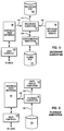
- Figure 2 depicts the playback and recording system interface to a recording file.
- Figure 3 depicts system interactions with the configuration subsystem.
- Figure 4 depicts system interactions with the data display subsystem.
- Figure 5 depicts system interactions with the recording subsystem.
- Figure 6 depicts system interactions with the playback subsystem.
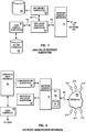
- Figure 7 depicts system interactions with the data value receiver subsystem.
- Figure 8 depicts system interactions with the network send/receive subsystem.
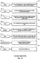
- Figure 9 is a flow diagram of the operations of the recording subsystem.
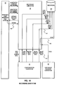
- Figure 10 depicts the recording subsystem interfaces to the overall performance tool system.
- Figure 11 is a table showing allowable actions from various menu selections.
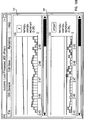
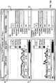
- Figures 12a-12e depict various displays generated by the performance tool.
- Figure 13 depicts the playback subsystem interfaces to the overall performance tool system.
- Figure 14 depicts concurrent operations between multiple data processing systems.
- Figure 15 is a flow diagram of the internal operations of the playback subsystem.
- Figure 16 is a flow diagram of the internal operations of the data display subsystem.
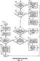
- Figure 17 is a flow diagram of the internal operations of the configuration subsystem.
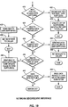
- Figure 18 is a flow diagram of the internal operations of the data value receiver subsystem.
- Figure 19 is a flow diagram of the internal operations of the network send/receive interface.
- Figure 20 is a flow diagram of the internal operations of the graphical user interface.
- Figure 21 depicts the graphical user interface subsystem interfaces to the overall performance tool system.
- Figure 22 depicts the interface between a data supplier daemon and a dynamic data supplier.
- Figure 23 is a flow diagram of the internal operations of the data supplier daemon.
- Figure 24 is a flow diagram of the internal operations of the xmpeek utility.
- Figure 25 depicts the data supplier daemon interfaces to the overall performance tool system.
- Figure 26 shows an example of output generated from the sample program listed in Appendix A.
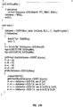
- Figure 27 is a C language program of a dynamic data supplier program using the daemon application programming interface to provide extensions for supplying additional types of data.
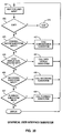
- Figures 28a-28b are flow diagrams of the internal operation for annotation and marking of data.
- Figure 29 is a flow diagram of the internal operation for a pathology library system.
- Figure 30 is a block diagram of the filtering and alarm capabilities of the performance tool.
- Figure 31 is a flow diagram of the internal operations of the filtering and alarm utility filtd.
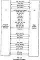
- Figure 32 depicts a data recording file having marker token for supporting annotations.
- Figure 33 depicts the preferred embodiment data processing system.
- the performance tool 90 can be perceived as consisting of five subsystems and two interfaces. The following sections describe each of these components.
- GUI 80 graphical user interface
- the performance tool's graphical user interface (GUI) 80 allows the user to control the monitoring process almost entirely with the use of a pointing device (e.g. a mouse or trackball).
- GUI 80 uses menus extensively and communicates directly to the following four subsystems:
- the GUI 80 allows the user to start and stop recording from any active monitoring console and any active monitoring instrument.
- recording begins in the recording subsystem 20, the configuration of the entire monitoring console is written to a recording file (100 of Figure 2).
- the recording file 100 itself is named from the name of the monitoring console from which it is being recorded.
- playback can be initiated without a lengthy interaction between user and playback subsystem 50.
- the GUI 80 the user can start and stop recording as required and if a recording file already exists when recording is requested for a monitoring console, the user is given the choice of appending to the existing file or replacing it.
- the configuration subsystem 30 has two means of acquiring information about the monitoring of consoles and instruments.
- a configuration file (110 of Figure 3) can contain configuration information for many monitoring devices. These may be skeleton consoles or may be fixed consoles.
- the user can add, change, and delete configuration about fixed consoles directly through the GUI 80. Whether configuration information is read from the configuration file or established in interaction with the user, it causes configuration messages to be exchanged between the configuration subsystem 30 and the network send/receive interface 70 and the remote data supplier daemon(s) (210 of Figure 8).
- the skeleton consoles are monitoring devices where the exact choice of the performance data to display is left open.
- the user To activate a skeleton console, the user must specify one or more instances of the available performance data, such as the processes, the remote host systems, or the physical disks to monitor.
- a new instance is created. This new instance allows a user to activate multiple, similar-looking consoles, each one monitoring different performance data, from one skeleton console.
- the user uses the GUI 80 to activate or close monitoring devices, thereby causing network messages to be exchanged between the configuration subsystem 30 and the network send/receive interface 70.
- These messages consist largely of instructions to the remote data supplier daemon(s) (210 of Fig. 8) about what performance data to send and how often.
- the data display subsystem 40 receives information about monitoring devices from the configuration subsystem 30 and uses this information to present the user with a list of monitoring devices for the user from which to select.
- the GUI 80 will also present a list of the items from which the user can select when instantiating the skeleton console.
- GUI 80 is used to start the playback of recordings at 50. Recordings are kept in disk files (recording file 100 of Figure 2) and may have been created at the same host system that is used to play them back, or may have been generated at other hosts. This flexibility allows a remote customer or user to record the performance data for some workload and mail the performance data to a service center or technical support group to analyze.
- Recordings 100 contain all necessary information to recreate exact replicas of the monitoring consoles from which they were recorded.
- the imbedded configuration data is passed on to the data display subsystem 40 and a playback console is constructed on the graphical display.
- the playback console Once the playback console is opened, the user can play the recording at almost any speed, can rewind, search for any time stamp on the recording, erase the recording and stop the playback of the recording.
- the configuration subsystem 30 has several important functions in the performance tool: a graphical user interface 80, a configuration file 110, a network send/receive interface 70, and a data display subsystem 40. Each is closely related to one of the interfaces or other subsystems, as described below.
- GUI 80 Through the graphical user interface (GUI) 80, the user can design the monitoring devices to use, can instantiate skeleton consoles, can activate and close consoles, and can traverse the hierarchy of performance data available from any of the data supplier daemons (210 of Figure 4) in the network 200. This is done in close cooperation between the GUI 80, the configuration subsystem 30, and the network send/receive interface 70.
- GUI graphical user interface
- the GUI presents the user with a series of graphical menus that allow a user to completely specify the appearance and contents of a graphical performance "console.” Via the menu selections, the user can create a new "console” window, add new "instrument” subwindows, and add multiple instrument values to any instrument. Values are individual statistics being monitored, displayed and/or recorded, and include such statistics for system elements such as CPU, memory, paging space, disk, network, process, system call, system I/O, interprocess communications, file system, communication protocol, network file system, or remote procedure calls. The user also has menu control over the colors, value limits, presentation style, sampling frequency, labeling, and other value attributes.
- an ASCII configuration file 110 in "stanza" formats similar to Motif resource files. If the user wishes to access remote statistics, the remote nodes are contacted via the network send/receive interface 70 to ensure that they are available and have the requested statistics generally specified by "skeleton" consoles in the local configuration file. After the user has made these selections through the GUI, the requested console is displayed and live data is fed to the graphics console. When the user is finished viewing the console, it can be "closed” or “erased”. Closing a console leaves the console available in the configuration file 110 for later activation and viewing. Erasing a console removes the console from the configuration file, so that it must be reconstructed from scratch.
- the final configuration can be written to a configuration file 110, so that future invocations of the performance tool can obtain the configuration information by reading the file as the tool begins operations.
- the configuration file 110 is an important tool for the performance tool user.
- the file may contain three types of information:
- All configuration-type messages are of the "request/response" type. This is also true for the unique messages that allow a user to traverse the hierarchy of performance data to see what's available before selecting data to display in consoles.
- a "request-response” type protocol is a two way communication between a client and a server. The data client sends a "request for data” message to the data server and then waits for a "response" from the server. If the server does not respond within a specified time limit, the client may attempt a retry or terminate with an error.
- the configuration subsystem 30 supplies configuration information to the data display subsystem 40 whenever the user requests that a console be activated.
- the detailed console specifications that were originally read into memory from the configuration file 110 are passed to the data display subsystem 40 in a memory control block area.
- the configuration subsystem 30 can likewise pass skeleton console data that was read from the configuration file to the data display subsystem 40 in a memory control block area.
- the data display subsystem's 40 main responsibility is to display the performance data in the format described by the configuration subsystem 30, and to display it as soon as it is received from either the playback subsystem 50 or the data value receiver subsystem 60.
- the data display subsystem 40 interfaces to three other subsystems, 30, 50, 60, and the GUI 80.
- the data display subsystem 30 is primarily a receiver of information from two of the other subsystems; only the interface 120 to the GUI 80 and, to some extent, the configuration subsystem interface 122 are dialog type interfaces.
- the configuration subsystem 30 is a supplier of configuration information and a vehicle for traversing the hierarchy of the performance data.
- the former is used to construct the windows and subwindows of monitoring devices on the graphical display; the latter is used to present lists of choices when a skeleton console is created or when designing or changing an ordinary console.
- the traversal of the data hierarchy requires the exchange of network messages between the configuration subsystem 30 and the data supplier daemon(s) 210 involved, using the request/response network interface.
- requests to start, change, and stop feeding of performance data are passed from the data display subsystem 40 to the configuration subsystem 30 through the network send/receive interface 70 to the data supplier daemon 210 of Figure 4.
- Data flow on the interface 124 to the data value receiver subsystem 60 is unidirectional, always from the data value receiver subsystem 60 to the data display subsystem 40.
- the data value receiver 60 uses the StatSetID from the received packets to do a lookup in a list of all active display consoles from a common parameter storage area, gets a pointer to the console control block, and passes this information at 124 to the data display subsystem 40.
- the playback subsystem 50 mimics the data value receiver subsystem 60. Where the latter receives packets of data over the network, the playback subsystem 50 reads them at 126 from the recording file 100 and hands them at 128 to the data display subsystem 40 in the same data format that the data value receiver subsystem 60 uses. This allows the data display subsystem 40 to handle the two data sources as if they were the same.
- the recording subsystem 20 of Figure 5 is controlled from the GUI 80 over interface 140.
- the configuration information 110 is stored in the recording file 100.
- This configuration information 110 is extracted from the current in memory control blocks and consists of the following control blocks:
- the actual data recording uses a fifth and final control block format. This format allows for variable length blocks to be written to preserve file space.
- This design also keeps data volume requirements down by referring each data recording data block symbolically to the configuration information in the recording file, rather than storing long identifiers.
- the contents of each data block is described later, with reference to Table 5.
- the recording subsystem 20 will, for each console that has recording activated, be passed the actual data feed information at 142 as it is processed by the data value receiver subsystem 60. As long as recording is active for a console, data is passed along.
- the playback subsystem of Figure 6 has logic to permit a realistic playback from any recording file 100.
- the logic also allows searching for time stamps in a recording with data from many hosts, each of which had different clock settings when the recording was created.
- the playback subsystem 50 as seen from the data display subsystem 40, is just another supplier of data packets along 128.
- Packets are read from the recordings file 100 at the speed requested by the user at 130 and fed at 128 to the data display subsystem 40.
- the GUI 80 is the only other subsystem interfacing at 129 with the playback subsystem 50. It allows the user at 130 to:
- the data value receiver subsystem 60 of Figure 7 is responsible for receiving all data feed packets arriving from the network 200 and making sure all interested subsystems get a copy of each data feed packet. Before the packet is passed on, it is tagged with information that identifies the target console to which it is intended. If no target can be found, the data packet is discarded.
- the interface to the other subsystems and the network send/receive interface is as follows.
- the network send/receive interface 70 uses the API library functions (described later, with reference to 161 of Figure 8) to access the network 200. This includes the API callback function that gets control whenever a data feed package is received.
- the data value receiver subsystem 60 is the only function that will ever receive data packets at interface 150 in the performance tool. Subsystem 60 does not have to poll but is scheduled automatically for each data feed packet received.
- the communications at 150 with the network send/receive interface 70 is strictly unidirectional. Because of this unidirectionality and lack of polling/responses, data can be supplied along 150 at very high data rates, thus allowing for real time monitoring of remotely supplied statistics.
- the data value receiver subsystem 60 consults the tables of active consoles 156 as maintained by the data display subsystem 40. Data packets that can not be related to an active monitoring console are discarded, assuming they arrived after the console was closed. If a console is identified, the recording subsystem 20 is invoked if recording is active for it. Then the packet is passed on at 152 to the data display subsystem 40 where further decoding is done as part of the actual display of data values. This design thus provides the ability to concurrently display and record local and remotely supplied performance statistics in real-time.
- the recording subsystem 20 is invoked at 154 to write a copy of the data packet to the recording file 100. If recording is only active for some of the instruments in the console, only data belonging to those instruments is actually written to the recording file 100.
- the network send/receive interface 70 consists of (i) the library functions 161 of the performance tool's application programming interface (API) 160, and (ii) code written specifically for the performance tool's monitoring program to invoke the API library functions 161.
- API application programming interface
- the interface has several responsibilities, the most prominent of which are:
- recording of statistics can be initiated for one or more instruments in a console or for all instruments in a console. Recording can be active for more than one console at a time. All recordings from any one console always goes to a file in directory "$HOME/XmRec", which has a name prefix of "R.” followed by the name of the console. For example, the recording file for a console named "Remote IP Load" would be: $HOME/XmRec/R.RemoteIPLoad
- a console cannot be recorded while playing back from a file whose name matches the console.
- Fourth, recording files are located in a subdirectory named "XmRec" in the user's home directory. If this directory does not exist when recording is attempted, it is created if possible.
- Begin Recording This option will start writing data values to the recording file as they are received. It does not matter whether the data is received from a remote data supplier or is local. Recording continues until stopped by the user or the console is closed (as specified by 130, through the GUI 80). Save & Begin Recording Combines the previous two options by first saving the display history buffer data to the file; then starting recording. End Recording Stops recording and closes the recording file if no other instrument in the console is still recording.
- the recording file contains five types of records, each mirroring control blocks internal to the performance tool.
- the record types are the following:
- Table 1 describes the layout of the console record.
- This record contains information such as the left and top offset of the console (measured in pixels from the left side of the display), the height and width of the console window (in pixels), a count of the number of instruments within this console, and the major and minor protocol versions.
- the major and minor protocol version fields are used to identify different protocol versions across releases. If the recording format has major changes, the "major" protocol version number is incremented. Minor changes, or versions for different systems, would cause the "minor” protocol version number to be incremented. Thus, these fields allow the playback subsystem to identify recordings that are of a compatible level.
- This console information is written to the recording file at 176 ( Figure 9) if a new recording file is being created, as determined by 174.
- Table 2 For each instrument within the console being recorded, the information of Table 2 is written to the recording file 100, such that the format of the internal control block consistency is maintained between the subsystems. This information is written at 184 ( Figure 9) when a new recording file is being created, as determined at 182.
- the graph type indicates whether this is a monitor-type (i.e. fixed) or skeleton-type (created from a skeleton)
- the graph collection name is the name of the console to which this instrument belongs.
- the subgraph number indicates which positional instrument this is within the console.
- the offsets are the location of the instrument within the console, specified as a percentage of the height (for top and bottom offsets; top being 0%) and width (for left and right offsets; left being 0%).
- the number of pixels to shift specifies how many picture elements (pixels) to shift the time graphs between subsequent data recording observations.
- the space between bars parameter is the number of pixels to space between bar graph elements being displayed.
- the history parameter specifies the number of observations to save in the display buffer for an instrument.
- the display history buffer is a 'cache-like' buffer which maintains recent data displayed on the display.
- the time interval parameter specifies the data recording sampling frequency, in milliseconds. This time interval allows the granularity of samples to be varied in real time, and further allows for differing instruments to record the same value at different granularities, or frequencies.
- the index into tile array is a number that identifies a tile "pattern" in an array of tile patterns (e.g. vertical stripes, horizontal stripes, diagonal stripes, checkerboard, cross-hatch, etc.). These patterns can be combined with the foreground and background colors of a statistic being displayed to help differentiate it from other statistics in an instrument.
- the style parameter indicates the primary style of the instrument, such as a line graph, area graph, skyline graph, bar graph, state bar graph, state light graph, speedometer graph or pie chart.
- the stacked parameter specifies whether stacking is to be used for values that use the primary style
- the basic description of each of the values of an instrument is stored in a record type shown in Table 3.
- the svp field is used to identify the value within the instrument and to match the following two record types (defined in Tables 4 and 5) with this one.
- the field is interpreted as two 16-bit values, where one identifies the instrument and the other gives the relative value number within the instrument. Again, this same principle is used for the two record types described next.
- the r1 and r2 values allow for scaling of graphs to match the data being recorded/displayed. There is a threshold alarm value, to trigger an action as described below.
- the index into tile array provides for differing tile patterns to be used for the graph fill.
- the graph style saves the style of graph to be displayed on a subsequent playback.
- Weighting allows to average more than a single sampled value to include the result of multiple samples taken over a period of time, thus providing a way to stabilize/average widely varying data samples.
- the descending flag indicates an alarm is to be triggered when the sampled value drops below (as opposed to going above) the threshold value.
- the path, label, and color fields are self-explanatory.
- the contents of the record type of Table 4 might as well have been included in the former record type of Table 3.
- the current format is chosen because it matches the internal control block format of the performance tool (i.e. the same as blocks created from the configuration file by the configuration. There is one instance of this record type for each value defined in the console. The name and description of the value are self-explanatory.
- the data type field specifies the type of data that is recorded (e.g. counter (counts/time interval) or quantity data(Cumulative count)).
- the data format field specifies the internal format of the data (e.g. floating point, long word, short word, character, etc.).
- the instrument identifier field is an identifier value that tells which instrument to which this array of recorded values belongs.
- Count is the number of values contained in this record.
- the two time fields are self-explanatory, and are used to timestamp the values that were captured.
- the Instr_Def data structure defines an "array of data reads” that has "n” records (as specified by the "count” field), the records being of the format defined by the Per_Val_Rec structure shown in this Table 5.
- the recording subsystems interfaces of Figure 5 are further expanded in Figure 10.
- the interface 140 between the GUI 80 and the recording system 20 comprises messages from the GUI 80 to start/stop console recording and to start/stop instrument recording.
- the recording subsystem 20 can send a message to the GUI 80, to be presented to a user/operator of the performance tool, on whether the user desires to append or replace the recording file.
- the GUI 80 returns a yes/no user response in a message to the user.
- the interface 142 between the data value receiver subsystem 60 and the recording subsystem 20 comprises data blocks.
- the recording subsystem 20 does not have to worry with, or maintain, the origin of the data, as this operation is done by the data value receiver subsystem.
- the recording subsystem 20 also treats local and remote data statistics identically, further providing minimal overhead delays when recording data. This is because all data, whether local or remote, is treated the same by the data value receiver subsystem 60.
- data can be quickly recorded in real-time as the overhead for receiving a packet of data and storing in the recording file is minimal. Further, as the overhead is minimal, recording can occur concurrently with the display of data, as will be later described.
- the interface 141 between the recording subsystem 20 and the recording file 100 comprises the data to be recorded (described above), as well as the console, instrument, value display, and value detail information, thus maintaining the context of the stored recording data.
- This information (console, instrument, value display, and value detail) is obtained across interface 143 from the configuration subsystem 30, as initiated by a request for configuration information from the recording subsystem 20.
- playback 234 is initiated from the "File" 232 menu of the main window of the performance tool user interface 230, as shown in Figure 12a.
- the file list consists of all files in the "$HOME/XmRec" directory with a prefix of "R.”.
- a user can use the filter selection or button 248 and the filter portion of the file selection box at 242 to look for other masks in whichever directory they want.
- To select a file to replay a user clicks on it as indicated and then on the "OK" button 244 or double-clicks on the file name.
- the selection box will remain open after a user selects a file to replay. This allows the user to select more than one file. To make the selection box go away, a user clicks on "Cancel" 246.
- GUI instructs the playback system to open the file, as detected at 252.
- the performance tool reads the console configuration from the recording file and creates the console at 254 of Figure 15.
- the playback console is constructed from the console, instrument, value display, and value detail information records read in from the start of each recording (information structures described in Tables 1-4). This data is used to construct the playback console in the same manner that the data display subsystem constructs a regular console from data it reads in from the console configuration file.
- the main difference is that the creation of the playback console does not allow the normal console command pulldown or popup menus, but instead creates a special set of buttons to control the playback functions (e.g. Eject, Erase, Rewind, Seek, Play, Stop, Slower, and Faster), as shown in Figure 12c at 250. Playback doesn't start until a user clicks on the "Play" button.
- buttons as selected by a user are as follows: Eject Immediately stops playback, closes the console, and closes the playback file. To restart playback you must reselect "playback" from the "File” menu of the main window and reselect the playback file 100.
- the GUI 80 component gets notified via user controls 130 that the "Eject" button was depressed and sends a message to the playback subsystem 50 to stop the playback as detected at 256 ( Figure 15).
- the playback subsystem 50 then calls the data display subsystem 40 to remove the associated playback console and cleanup at 258 of Figure 15.
- the playback subsystem 50 closes the associated recording file 100 and exits.
- Erase Allows a user to erase a playback file.
- a dialog window will pop up.
- the dialog window warns that the user has selected the erase function, and indicates the name of the file currently playing back from.
- a user selects "OK”.
- a user selects "Cancel”.
- the GUI 80 component gets notified via user controls 130 that the "Erase” button was depressed and sends a message to the playback subsystem 50.
- the playback subsystem 50 sends a message to the GUI 80 to display a dialog window to inform and solicit a response from the user. The user is prompted to confirm the erasure of the recording file 100 or cancel their request.
- the playback subsystem 50 will delete the recording file 100 at 282 ( Figure 15) and then call the data display subsystem 40 to remove the associated playback console from the display and cleanup.
- Rewind Resets the console by clearing all instruments and rewinds the recording file 100 to its start. Playback does not start until a user selects "Play”.
- the "Rewind" button is not active while playback is ongoing.
- the GUI component 80 gets notified via user controls 130 that the "Rewind" button was depressed. The GUI sends a message indicating this selection to the playback subsystem 50.
- the playback subsystem 50 detects this (268 of Figure 15) and sends a message to the data display subsystem 40 to reset all the console instruments back to their initial state (270 of Figure 15).
- the playback subsystem then resets a pointer to the beginning of the recording file 100.
- the playback of a recording does not start until a user selects the "Play" menu button. Seek User selection of "Seek” pops a dialog box that allows a user to specify a time desired to seek for in the playback file 100. The time can be set by clicking on the "Hour” or “Minute” button. Each click will advance the hour or minute by one. By a user holding the button down more than one second, the hour or minute counter advances faster.
- the GUI 80 component gets notified via user controls 130 that the "Seek" button was depressed and sends a message to the playback subsystem 50.
- the playback subsystem 50 sends a message to the GUI component 80 to display a dialog box to allow the user to specify a recording time to "seek to".
- Each data element in a recording has a timestamp that was affixed to the data value when the data was gathered by the data supplier.
- the recording subsystem 20 records the data, it preserves the original timestamp.
- the GUI 80 passes this parameter to the playback subsystem 50.
- the playback subsystem 50 detects this at 272 ( Figure 15) and then calls the data display subsystem 40 to reset the recording console instruments to their initial value.
- the playback subsystem then opens the recording file 100, reads in the graphical context of the recording, passes this data to the data display subsystem 40, and reads recording data from the recording file until it finds the specified "seek to" time.
- the playback system 50 reads the recorded data into memory, it checks the timestamp of each data entry and can thus seek to a particular point in time of a recording.
- the playback subsystem then sets the playback time pointer to this "seeked" data record at 274 ( Figure 15), and then waits for the user to select, via GUI 80, the "Play” button to start the playback from this recording time record.
- the seek proceeds from the current position in the playback file and wraps to the beginning if the time is not found. Because multiple data records may exist for any hour/minute, "Play” should be used to advance to the next minute before doing additional seeks on the same time, or seek for a time one minute earlier than the current playback time.
- the "Seek" button is not active while playing back. Play Starts playing from the current position in the playback file.
- the button's text changes to "Stop” to indicate that playing can be stopped by clicking the button again.
- the current position will be the beginning of the playback file. The same is true after a rewind.
- the GUI 80 component gets notified via user controls 130 that the "Play” button was depressed and sends a message to the playback subsystem 50.
- the playback subsystem 50 detects this at 260 and tells the GUI subsystem 80 to change the "Play" button to a "Stop” button and then starts to feed the data display subsystem 40 with recording data from the current position of the recording file at 262 ( Figure 15). Initially, playing back is attempted at approximately the same speed at which the data was originally recorded.
- the speed can be changed by using the "Slower” and “Faster” buttons. While playing back, neither the “Rewind” nor the “Seek” buttons are active.
- the playback subsystem 50 continues to feed recording data to the data display subsystem 40 until it reaches the end of the recording file 100, or the user presses the "Stop” button via user controls 130. If the user presses the "Stop” button, the GUI 80 is notified and sends a message to the playback subsystem 50. If “Stop” is signalled, the playback subsystem 50 tells the GUI to change the "Stop” button to a "Play” button and then stops feeding the data display subsystem 40 with recording data. The playback subsystem 50 then waits for an indication that the user has selected another action.
- the GUI 80 gets notified that the "Slower” button was depressed via user controls 130, and sends a message to the playback subsystem 50, where it is detected at 276 ( Figure 15).
- the playback subsystem 50 divides its playback rate parameter in half at 278 ( Figure 15), so that it now feeds the data to the data display subsystem 40 at half its present rate, thus providing a variable playback rate.
- the GUI 80 gets notified that the "Faster” button was depressed via user controls 130, and sends a message to the playback subsystem 50, where it is detected at 276 ( Figure 15).
- the playback subsystem 50 doubles its playback rate parameter at 278 ( Figure 15), so that is now feeds the data to the data display subsystem 40 at double its present rate, thus providing a variable playback rate.
- 00:00:00 At the far right of a console is a digital clock. It shows the time corresponding to the current position in the playback file 100 or zeroes if at the beginning of the file 100. As play back proceeds, the clock is updated. This is done by reading the time stamp associated with the playback data being read from the recording/playback file.
- FIG 13 further expands the interfaces of the playback system shown in Figure 6.
- the interface 129 between the GUI 80 and the playback subsystem 50 comprises a message initiated by an operator to open/close a recording.
- the playback subsystem responds to the GUI with a list of recordings available and the user's selection is returned from the GUI to the playback subsystem. Further messages from the GUI, as initiated by an operator, are to play/stop, rewind, seek, slower/faster and erase a recording file 100.
- the interface 126 between the recording file 126 and the playback subsystem 50 provides the actual data to be displayed on a computer console, such as that shown in Figure 12c. Further information read from the recording file 100 includes console, instrument, value display and value detail information. Again, this information is used to preserve the display context of the data to be presented to a user.
- All information and data read at interface 126 is passed immediately to the data display subsystem 40 at interface 128.
- Minimal system overhead is required to read the data and display it, allowing for other subsystem activities to occur with the actual displaying of data, such as recording the same or other performance data.
- a linear media such as a magnetic tape
- This arrangement is quite inflexible and does not allow functions like rewind, search, faster, slower, or play/stop while recording.
- recording is done on a filesystem that allows concurrent reading writing to a common file. Therefore, the record and playback functions are more independent in their operations than those of a linear media.
- the record function can continuously record prespecified data while a playback function can simultaneously read the data already recorded, up to the currently recorded data record, without disturbing the recording process.
- a copy of the recording file is made to another file, then the playback can be done totally concurrently and independently of the original recorded file.
- Another technique that can be used is to copy the context of the data to be recorded and create two recording sessions for the same data. Then, a playback session can be invoked on one session while the other session continues recording of data. As shown in Figure 14, this technique can similarly be extended to multiple remote machines 218, such that any machine 201 is recording data while any other machine 203 is currently playing back the data from the same data source 210 on remote machine 218. This technique is feasible since a single data source 210 can feed multiple consumer applications concurrently. Further, data consumer and data supplier can coexist on a single machine 219, and similarly supply other data consumers and data suppliers in the network. One example of a combined data consumer and data supplier will be described later in the discussion on filters and alarms.
- An instrument occupies a rectangular area within the window that represents a console.
- Each instrument may plot up to 24 values simultaneously in the preferred embodiment, with the reading of all values taken at the same time. All values in that instrument must be supplied from the same remote host. This allows for live displays/recordings of statistics from remote hosts, as the processing overhead is minimized by maintaining this restriction.
- the ability to dynamically add, change, or delete multiple data statistics to a monitoring instrument is a very powerful usability aid in visualizing the correlation between nominally disjoint parameters.
- This combinatorial feature coupled with the ability to display each parameter in a different color and presentation style (e.g., line, bar, area, skyline, etc.) in a live time graph allows a very complex presentation of data that can still be comprehended with a minimum of explanation.
- a console of instruments can be constructed to show data from local and remote hosts, including statistics on individual processes.
- custom data from applications that have registered with the Data Server daemon can be added to the viewing instruments that show normal system statistics (also from local or remote hosts). All of these operations can be done while the instruments are receiving data from the data supplier(s) and the display views are updated in real time (live). Data values of the same primary style can also be stacked and unstacked without disturbing the reception of data.
- a recording graph/instrument shows statistics for a system resource over a period of time, as shown at 249 in Figure 12d. Recording graphs have a time scale with the current time to the right. The values plotted are moved to the left as new readings are received.
- a state graph/instrument 251 of Figure 12e shows the latest statistic for a system resource, optionally as a weighted average. They do not show the statistics over time, but collect this data in case it is desired to change the graph to a recording graph.
- History The number of observations to be maintained by the instrument. For example, if the interval between observations is 2,500 milliseconds and you have specified that the history is 1,000 readings, then the time period covered by the graph will be 1,000 x 2.5 seconds or approximately 42 minutes.
- the history property has a meaning for recording graphs only. If the current size of the instrument is too small to show the entire time period defined by the history property can be scrolled to look at older values. State graphs show only the latest reading so the history property does not have a meaning for those.
- Stacking works only for values that use the primary style. To illustrate, think of a bar graph where the kernel-cpu and user-cpu time are plotted as stacked. If at one point in time the kernel-cpu is 15% and the user-cpu is 40%, then the corresponding bar will go from 0-15% in the color of kernel-cpu, and from 16-55% in the color used to draw user-cpu. If it is desired to overlay this graph with the number of page-in requests, one could do so by letting this value use the skyline graph style, for example. It is important to know that values are plotted in the sequence they are defined. Thus, if a user wanted to switch the cpu measurements above, they would simply define user-cpu before defining kernel-cpu.
- four properties determine the relative position of an instrument within a console. They describe, as a percentage of the console's width and height, where the top, bottom, left and right sides of the instrument are located. In this way, the size of an instrument is defined as a percentage of the size of the monitor window.
- the relative position of the instrument can be modified by moving and resizing it as is commonly done in a MOTIF-like user interface, and as described below.
- Each state light may be in one of two states: Lighted (on) or dark (off).
- the value is shown with the label background in the instrument's background color and the text in the instrument's foreground color. Notice that if the instrument's foreground and background colors are the same, one would see only an instrument painted with this color - no text or label outline is visible. If the two instrument colors are different, the labels will be seen against the instrument background and label texts are visible.
- the instrument's background color is used to paint the text while the value color is used to paint the label background.
- the special use of colors for state lights allows for the definition of alarms that are invisible when not triggered - or alarms that are always visible. The colors chosen depend on the selections made during setup.
- Some computer system objects change over time.
- One prominent example of these changes is the set of processes running on a system. Because process numbers are assigned by the operating system as new processes are started, it is not known what process number an execution of a program will be assigned. Clearly, this makes it difficult to predefine consoles and instruments for processes in the configuration file.
- Skeleton instruments are defined in the configuration file as having a "wildcard" in place of one of the hierarchical levels in the path that define a value.
- a user could specify that a skeleton instrument for processes which have the following two values defined: Proc/*/kern Proc/*/user
- the wildcard is represented by the asterisk. In the above example, it appears in the place where a fully qualified path name would have a process ID. Whenever users try to start a console with such a wildcard, they are presented with a list of processes. From this list, the user can select one or more processes. Each process selected is used to generate a fully qualified path name. Each path name is then used to define either a value to be plotted or define a new instrument in the console.
- Skeleton instruments are also useful for handling the problem of varying resource configurations across different systems or over time.
- a skeleton instrument could be defined in which the disk name was replaced by a wildcard, to permit monitoring of any disk configuration on any system.
- the type of skeleton defined determines which one is selected. There are two types of skeletons, as described in the following sections.
- the skeleton type named "All" is so called because an instrument of this type will include all instances of the wildcard which are selected into the instrument. In the case of processes, this would include all selected processes.
- a skeleton instrument creates one instance of an instrument and this instrument contains values for all selected processes.
- Consoles may be defined with both skeleton instrument types but any non-skeleton instrument in the same console will be ignored.
- the relative placement of the defined instruments is kept unchanged. This may result in very crowded instruments when many processes are selected, but it is easy to resize the console.
- the performance tool will not resize the console.
- the type of instrument best suited for "All" type skeleton instruments is the state bar, but other graph types may be useful if the user chooses to allow colors to be assigned to the values automatically. To do the latter, the color is specified as "default" by the user when the skeleton instrument is defined.
- each skeleton type is so named because each instance of the wildcard object which is selected will create one instance of the instrument. In the case of processes, when five processes are selected by a user, each of the type "Each" skeletons will generate five instruments, one for each process.
- one console may define more than one skeleton instrument and consoles can be defined with both skeleton instrument types, while any non-skeleton instruments in the same console are ignored.
- the relative placement of the defined instrument is kept unchanged. This may result in very small instruments when many processes are selected, but it's easy to resize the console. If the generated instruments would otherwise become too small, the performance tool will attempt to resize the entire console.
- Wildcards must represent a section of a value path name which is not the end point of the path. It could represent any other part of the path, but it only makes sense if that part may vary from time to time or between systems. With the standard statistics, the following wildcards are used: PagSp/*/... Page Spaces Disk/*/... Physical disks NetIF/*/... Network (LAN) interfaces Proc/*/... Processes hosts/*/... Remote hosts
- An extension to the concept of single wildcard notation is to use multiple wildcards to specify all statistics for a class of system objects.
- This facility permits users to define generic skeleton consoles for monitoring classes of system objects (eg. disks, processes, paging spaces, network hosts, etc.), without requiring users to identify specific instances of the class.
- skeleton consoles can then be instantiated at run-time to monitor whatever system objects exist on a particular machine or set of network machines at a particular time (e.g., hdisk0, X process, /dev/hd6, abc.aus.ibm.com, etc., for all subnet nodes).
- skeleton consoles are defined in a text configuration file by specifying the following information:
- the above line has the information for the performance tool to monitor the working memory use of specific processes on multiple host machines.
- the host name and process ID are replaced with an asterisk (e.g., */Proc/*/workmem) to indicate to the performance tool that the particular hosts and processes are determined when the monitor is opened.
- the performance tool determines the common part of the name from the value names displayed in the instrument and displays the common part in a suitable place. In determining how to do this, the performance tool examines the names of all values in the containing console. To illustrate, assume a single instrument is in a console, and that this instrument contains the values: PagSp/paging00/%free PagSp/hd6/%free
- the first instrument has the values: Mem/Virt/pagein Mem/Virt/pageout while the second instrument has: Mem/Real/%Work Mem/Real/%free
- the second instrument would display "Real” in reverse video and use the value names: %work %free
- Consoles like instruments, are rectangular areas on a graphical display. They are created in top-level windows of the OSF/Motif ApplicationShell class, which means that each console will have full OSF/Motif window manager decorations. These window decorations allow you to use the mwm window manager functions to resize, move, iconify, and maximize the console.
- the window manager Close function invokes the Exit xmperf function also available from the File menu.
- Consoles are useful "containers" for instruments.
- a user can:
- Consoles may contain non-skeleton instruments or skeleton instruments but not both. Consequently, it makes sense to classify consoles as either non-skeleton or skeleton consoles. The two work a little differently, as will now be described.
- Non-skeleton consoles may be in one of two states: open or closed.
- a console is opened by a user selecting it from the Monitor Menu. Once the console has been opened, it may be iconified, moved, maximized, and resized through mwm. None of these actions change the status of the console. It may not be visible on the display, but is is still considered open and if recording has been started, it continues.
- the name of the console on the Monitor Menu is now preceded by an asterisk. This indicates that the console is open. If a user selects on one of the names preceded by an asterisk, the corresponding console is closed.
- Skeleton consoles themselves can never be opened.
- a user selects one from the Monitor Menu, it is not opened, but rather causes the display of a list of names matching the wildcard in the value names for the instruments in the skeleton console. If a user selects one or more from this list, a new non-skeleton console is created and added to the Monitor Menu. This new non-skeleton console is automatically opened, and is given a name constructed from the skeleton console name suffixed with a sequence number.
- Skeleton consoles are defined like any other console. Neither the keywords defining the console nor those defining the instruments are different. The only difference is in one keyword used to define the values in the instruments of the console. The keyword that is different is "input" keyword, which must be changed to one of "all" or "each".
- monitor.Single-host Monitor.3.each.1 hosts/*/CPU/kern monitor.Single-host Monitor.3.each.2: hosts/*/Syscall/total monitor.Remote Mini Monitor.1.each.4: NetIf/*ipacket monitor.Remote Mini Monitor.1.each.5: NetIf/*/opacket monitor.Disk Monitor.1.all.1: Disk/*/busy
- skeleton types within a console can be mixed and that all paths up to the wildcard must be the same, not only in an instrument but for all instruments in a console.
- Skeleton instruments of type "all” can, as has already been pointed out, only have one value defined. It follows that all values in the instantiated instrument will have the same color, namely as defined for the value in the skeleton instrument. This is rather dull. Worse though, is that it effectively restricts the "all" type skeletons to use the state bar graph type since otherwise you wouldn't be able to tell one value from another.
- the non-skeleton console created from the skeleton is said to be an "instance" of the skeleton console; a non-skeleton console has been instantiated from the skeleton.
- the instantiated non-skeleton console works exactly as any other non-skeleton console, except that changes a user may make to it will never affect the configuration file. A user can close the new console and reopen it as often as desired, as well as resize, iconify, maximize, and resize it.
- a skeleton console is selected from the monitor Menu, a new instantiation is created, each one with a unique name. For each instantiation, the user is prompted to select values for the wildcard, so each instantiation can be different from all others.
- the easiest way to change and save is to use the "Copy Console" function from the console menu. This will prompt a user for a name of the new console and the copy will be a non-skeleton console looking exactly as the instantiated skeleton console copied from. Once the console has been copied, a user can delete the instantiated skeleton console and save the changes in the configuration file.
- All consoles are defined as OSF/Motif widgets of the XmForm class and the placement of instruments within this container widget is done as relative positioning.
- the instrument goes away and is replaced by a rubber-band outline of the instrument.
- a user resizes the instrument by holding mouse button 1 down and moving the mouse. When the user presses the button, the pointer is moved to the lower right corner of the outline and resizing is always done by moving this corner while the upper left corner of the outline stays put.
- the position of the resized instrument must be rounded so that it can be expressed in percentage of the console size. This may cause the instrument to change size slightly from what the rubber-band outline showed.
- Instruments cannot be resized so that they overlap other instruments. If this is attempted, the size is reduced so as to eliminate the overlap.
- the instrument When an instrument is selected to be moved, the instrument disappears and is replaced by a rubber-band outline of the instrument.
- a user places the mouse cursor within the outline and presses the left mouse button. The button is held down while moving the mouse until the outline is at the desired location. Then, the button is released to redraw the instrument.
- Instruments can be moved over other instruments, but are never allowed to overlap them when the mouse button is released. If an overlap would occur, the instrument is truncated to eliminate the overlap.
- the data display subsystem 40 takes inputs from the GUI subsystem 80, data value receiver subsystem 60, and the playback subsystem 50 and creates the displays needed to show the performance data in the format described by the configuration subsystem 30. It calls the configuration subsystem 30 to get the display format information from the configuration files and also to send requests for system configuration information to Data Supplier daemons 210.
- the data display subsystem checks if data was received from the data value received or playback subsystems at 300.
- the input data format from each of these subsystems will be identical, so no special code is necessary to distinguish where the data originated. It picks up the pointer to the display data and the corresponding console from the input parameters and updates the data in the display console instrument at 302, and then exits.
- the data display subsystem was either invoked from the playback subsystem at 262 of Figure 15, where an operator has requested to "Play" the data, or data is sent from the data value receiver subsystem at 408 of Figure 18.
- the data display subsystem has minimal overhead to display statistical data, and the data display subsystem is able to present data from either a local or remote host with minimal impact on the system.
- the GUI subsystem would capture that input and pass it to the Display subsystem. If the selection was for a fixed console as determined at 306, then the configuration subsystem would be called at 308 to get the console configuration data to create the display console.
- the negotiation for statistics with data suppliers at 310 is initiated from the data display subsystem, but uses the configuration subsystem to obtain the data through the network send/receive interface.
- the Display Subsystem then would create and open the fixed display console at 312. It would then call the Network Send/Receive Interface to start the data feed from the Data Supplier Daemon at 314, and exit.
- the Data Display Subsystem would call the Configuration subsystem to get the console configuration data at 316, and then call the Network Send/Receive Interface to get the current skeleton parameters at 318, as specified by the skeleton template in the configuration file. Then it calls the GUI subsystem with the skeleton parameters to allow the operator to select which skeleton consoles they wish to view at 320. After receiving the operator choices from the GUI subsystem, it calls the Configuration subsystem to send a request to instantiate the skeleton console parameters to the Data Supplier Daemon(s) via the Network Send/Receive Interface. After receiving the data from the Data Suppliers, it creates and opens the skeleton display console at 322. Finally it sends a "start data feed" request to the Data Supplier daemon(s) via the Configuration and Network Send/Receive Interface subsystems at 314, and exits.
- GUI subsystem would pass that input to the Data Display subsystem.
- the Data Display subsystem would then send a "stop data feed” request to the Data Supplier Daemon(s) via the Configuration and Network Send/ Receive interface subsystems at 326. Finally, it would close the Display Console at 328 and exit.
- the GUI subsystem would capture that input and pass it to the Data Display subsystem together with the new graph style options selected.
- the Data Display subsystem would then change the display modes dynamically so that the current console, instrument, and value attributes would be updated and displayed with the new values at 342.
- the configuration file would not be updated until the operator explicitly requested the configuration file to be saved.
- GUI subsystem would pass that input to the Data Display subsystem to open a tabulation window for the selected instrument at 346, and set a flag for the data values to be displayed in this window concurrently with the graphic data in the corresponding instrument at 348.
- the GUI subsystem calls the Data Display subsystem which then calls the configuration subsystem to get the command string from the configuration file at 352. It also gets user supplied parameters at 354 and then it passes the command string to the host operating system to execute the command string at 356.
- the playback file is opened and the console configuration data that had been previously saved is read at 358.
- a playback console is opened on the display at 360, using this console configuration data. This action is initiated by the playback subsystem at 254 of Figure 15, and provides the ability to automatically present the operator with the previously recorded data in the same context in which it was originally recorded, without requiring extensive operator interactions for setup of the context.
- data recording feeds are initiated at 362, where a request is sent to data suppliers to start data feeding. Data feeds received as a result of this request are processed at 302.
- the main functions of the Configuration Subsystem 30 are to take requests for data from the configuration file 110 and return requests or data to the caller. It also is the main interface to the Network Send/Receive Interface 70 to route data requests to the proper Data Suppliers.
- the configuration subsystem parses the configuration file and builds the initial configuration definition control blocks that determine how all the monitor and menus will look when created.
- the Console subsystem retrieves that data from the configuration definition control block and returns that data to the caller at 372.
- the GUI subsystem will pass this request to the Configuration subsystem at 360 ( Figure 17), which will then rename the current configuration file with a timebased name and then write the current configuration control block data to a new file that will be the active configuration file at 362, and then exit at 390.
- GUI needs to present the operator with a list of network nodes, it calls the configuration subsystem at 364 to send this request to the Data Supplier daemons via the Network Send/Receive interface at 366. As the Data Suppliers respond to the request, a list of responding nodes is created and returned to the GUI subsystem at 368.
- a caller routine requests a "start”, “stop”, or “change data feed rate” be sent to the data supplier(s) as determined at by 374 and 380
- the configuration subsystem sends this request to the Data Suppliers(s) via the Network Send/Receive Interface at 386, and then exits at 390.
- the configuration subsystem sends this request to the Data Supplier(s) via the network send/receive interface at 382 and returns the data received to the caller at 384.
- An example of a data context hierarchy is:
- a program would call RSiInstantiate to create (instantiate) all subcontexts of a context object.
- RSiPathGetCx to search the context hierarchy for a context that matches a path name.
- RSiFirstCx to return the first subcontext of a context.
- RSiNextCx is called to get the next subcontext of a context.
- Statistics are at the leaf nodes of the context hierarchy. The statistics can be retrieved by calling RSiFirstStat to get the first statistic of a context and RSiNextStat gets the next statistics of a context.
- the data value receiver subsystem 60 of Figure 7 receives all data feeds at 150 from the Network Send/Receive Interface 70.
- This data includes the StatSetID so that the incoming data can be matched to a specific instrument in an active display console.
- the data value receiver upon receipt of a data feed packet 400, gets the StatSetID and searches the list of active display consoles looking for a matching StatSetID at 402. If the data value receiver does not find a match, it discards the data at 406.
- the data display subsystem If it finds a matching console, as determined at 404, it passes the data to the data display subsystem with a pointer to the console control block that it found at 408. If recording is active for the console or instrument, as determined at 410, then the data is also passed to the recording subsystem with a pointer to the console control block for the data to be saved in the recording file at 412.
- the main functions of the Network Send/Receive Interface 70 of Figure 8 are to send network requests to Data Suppliers 210, receive their responses, and to pass data feed information to the Data Value Receiver Subsystem 60.
- the network send/receive interface receives a call to identify all the data supplier daemons as determined at 420, the network send/receive interface broadcasts an "are_you_there" message to all the hosts in the local subarea network and any hosts specified in the hosts file at 422. The network send/receive interface waits for all the responses and then returns a list of all the responding hosts to the calling routine at 424.
- the Network Send/Receive interface receives a call to traverse a data hierarchy 426, negotiate an instrument data value 428, start, stop or change frequency of a data feed 430, it sends a request packet to the data supplier(s) daemons at 432, 434, or 436, respectively, waits for the response(s), and passes the response back to the configuration subsystem at 438 and 440.
- the data supplier daemon 210 can be at either a local or remote node.
- the underlying TCP/IP socket communication protocol masks the daemon location from the data requestor. The data requestor only specifies a node name and the communication protocol determines whether it is local or remote.
- the network send/receive interface receives a data feed from a data supplier daemon at 442, therefore passes the data to the Data Value Receiver subsystem at 444.
- the graphical user interface 80 is simply an interface between a user and the performance tool, receiving user input and passing the information on to the appropriate performance tool subsystem.
- the interface waits to receive user input at 421.
- a check is then made if the user desires to exit the performance tool at 423. If so, the tool is terminated at 419.
- processing continues at 425, 429, 433 and 437, where checks are made to determine if the input is destined for the configuration, data display, recording, or playback subsystems, respectively.
- the appropriate subsystem is called at 427, 431, 435 or 439, based upon the destination of the user input.
- the GUI interface to the recording system consists of the following.
- a user initiates a request to start/stop a console or instrument recording, which the GUI detects at 433 ( Figure 20) and sends to the recording subsystem.
- the recording subsystem sends a message to the GUI to prompt the user whether the user desires to append/replace an existing recording file and the user response to such inquiry is returned to the recording subsystem.
- the GUI interface to the configuration subsystem comprises the following messages.
- a user initiated message to create/erase/copy a console can be sent to the configuration subsystem.
- a request to initiate a console can also be sent, with a response from the configuration subsystem being a message listing possible console instantiations.
- the user would then select from the list using the GUI, resulting in a message being sent from the GUI to the configuration subsystem indicating the selected instatiation(s).
- the user can also initiate a message to be sent to add an instrument, or to add/change a value, both of which result in a list of possible values to be presented to the user using the GUI.
- the user selects a value to be sent to the configuration subsystem.
- a user can initiate a request to save a configuration file.
- the GUI interface to the data display subsystem comprises the following messages.
- a user can initiate a request to open/close a console.
- a user can initiate a message to change the instrument style or properties, or to change the value properties.
- the data display subsystem sends the GUI a message containing a list of possible choices to present to the user, whereupon the user makes a selection to be returned to the data display subsystem.
- the GUI interface to the playback subsystem comprises the following messages.
- a user can initiate a message to instruct the playback subsystem to open/close a recording, and the playback subsystem responds with a list of recordings to be presented to the user for selection. The selection is returned to the playback subsystem.
- the user can also invoke actions which cause the GUI to send the playback subsystem various messages to play/stop, rewind, seek, play slower/faster, and erase a recording/playback file.
- the concept of separating the data collecting executable 210 from the data display executable 90 led to the concept of using a separate data supplier 220 capable of supplying statistics to data consumers 90 on a local 208 or on remote hosts 218.
- the performance tool 90 provides true remote monitoring by reducing the executable program on the system to be monitored remotely to a subset of the full performance tool.
- the subset, called xmservd 210 consists of a data retrieval part 207 and a network interface 205. It is implemented as a daemon that can be started manually, started from one of the system start-up files, or left to be started by the inetd super-daemon when requests from data consumers are received.
- the obvious advantage of this approach is that of minimizing the impact of the monitoring software on the system to be monitored. Because one host can monitor many remote hosts, larger installations may want to use dedicated hosts to monitor many or all other hosts in a network.
- the xmservd daemon can be ported to multiple (and differing) platforms, provisions are made to allow flexible adaptation to characteristics of each host where the daemon runs. This has several implications.
- the data supplier daemon 210 does not have any system dependent statistics imbedded in itself.
- the system dependent statistics and functions to extract such statistics are provided in external executables 220.
- a protocol and method of cross-accessing statistics between these external executables and xmservd is defined.
- an application programming interface is used to generalize the protocol and access mechanism. Thus, a customized tool similar to the performance tool described herein could be developed, and interface to the existing xmservd daemon.
- data supplier host 218 describes a host that supplies statistics to another host, while a host receiving, processing, and displaying the statistics is called a data consumer 208.
- the performance tool will attempt to contact potential suppliers of remote statistics in three situations, namely:
- the five-minute limit is implemented to make sure that the data consumer host 208 has an updated list of potential data supplier hosts 218. This is not an unconditional broadcast every five minutes. Rather, the attempt to identify data supplier hosts is restricted to times where a user wants to initiate remote monitoring and more than five minutes have elapsed since this was last done.
- the five-minute limit not only gets information about potential data supplier hosts that have recently started; the limit also removes from the list of data suppliers such hosts which are no longer available.
- the performance tool uses one or more of the following methods to obtain the network address(es) where an invitational are_you_there message can be sent.
- the last two methods depend on the presence of the file /usr/lpp/xmservd/hosts.
- the three ways to invite data supplier hosts are:
- Table 6 further shows that the hosts to monitor do not necessarily have to be in the same domain or on a local network.
- Table 7 illustrates a situation where it is desired to broadcast on all local interfaces, to broadcast on the subnet identified by the broadcast address 129.49.143.255, and also to invite the host called umbra.
- the xmservd daemon 210 is designed to be started from the inetd "super daemon". The following sections describe how xmservd starts, terminates, and keeps track of data consumer programs.
- the xmservd daemon 210 must be configured as an inetd daemon to run properly. If the daemon is manually started, it attempts to reschedule itself by invoking the program xmpeek and then exit. This will cause xmservd to be rescheduled via inetd.
- the line defining the daemon in /etc/inetd.conf must specify the "wait" option to prevent inetd from starting more than one copy of the daemon at a time.
- the xmservd daemon is started by inetd immediately after a UDP datagram is received on its port. This is because inetd has been setup during the preliminary system configuration to specify that the xmservd daemon should be started when these datagrams are received. Note that the daemon is not scheduled by a request through the SMUX interface from the local SNMP agent (this interface is described later). The SNMP agent uses a different port number. Unless xmservd abends or is killed, it will continue to run as long as any data consumer needs its input or a connection to the SNMP agent is established and alive.
- the daemon Whenever a connection to the SNMP agent through the SMUX interface is active, the daemon will not time-out and die even when there are no data consumers to supply. Then, the "time_to_live" limit is used only to determine when to look for inactive remote consumers that can be deleted from the tables in xmservd.
- xmservd will interpret the receipt of the signal SIGHUP (kill -1) as a request to refresh itself. It does this by spawning another copy of itself via inetd and killing itself. When this happens, the spawned copy of xmservd is initially unaware of any data consumers that may have been using the copy of xmservd that received the signal. Consequently, all data consumer programs must request a resynchronizing with the spawned daemon to continue their monitoring.
- SIGHUP kill -1
- the other signal recognized by xmservd is SIGINT (kill -2) that will cause the daemon to dump any MIB data.
- a data consumer program such as the performance tool 90
- time_to_live is used to check for inactive partners. A data consumer is removed from the daemon's tables if either of the following conditions are true:
- xmservd Once xmservd is running and supplying input to one or more data consumers as shown in Figure 23, it must make sure that the data consumers are still alive and needing its input. If not, xmservd would waste system resources to continue sending statistics across the network.
- the daemon uses an "alive limit" to determine when it's time to check that data consumer hosts are still alive. The alive limit is reset whenever the user makes changes to the remote monitoring configuration from the data consumer host, but not when data is fed to the data consumer.
- the xmservd daemon While in a quiescent state, the xmservd daemon is waiting either to receive a message or for the expiration of the "alive limit" at 450. Then, a check is made to determine if the requested action is the receipt of message in response to a previously sent still_alive message at 452. If so, the alive limit timer is reset at 454.
- xmservd When the alive limit is reached at 456, xmservd sends a message of type still_alive to the data consumer at 460.
- the data consumer program has "alive limit" seconds to respond. If a response is not received after "alive limit” seconds, as determined at 458, the daemon sends another still_alive message at 460 and waits another "alive limit” seconds at 450. If there's still no response, the daemon assumes the data consumer to be dead or no longer interested and stops sending statistics to the consumer at 462.
- the default "alive limit" is 300 seconds (five minutes); the alive limit can be set with the -t command line argument to xmservd.
- exception conditions can be defined that can cause one or more actions to be taken.
- One such action is the execution of a command on the host where the daemon runs; another is the sending of an exception message.
- the message type except_rec is used for the latter.
- the xmservd daemon will send exceptions to all hosts it knows that have declared that they want to receive exception messages.
- the RSiOpen and RSiInvite function calls of the API are used by the data consumer application to declare whether it wants to receive exception messages.
- the performance tool always requests exception messages. When one is received, the exception message is sent to the performance tool main window where it appears as a text message. No other action is taken by the performance tool.
- the daemon will attempt to record the connections in the file /usr/lpp/xmservd/xmservd.state (the xmservd command line argument -d can be used to substitute a different directory for /usr/lpp). If this file exists when xmservd later is restarted, a message of type i_am_back is sent to each of the data consumer hosts recorded in the file. The file is then erased.
- the interrupted monitoring can resume swiftly and without requiring manual intervention.
- the performance monitor can and does resynchronize all active monitors for a host whenever an i_am_back message is received from that host, by renegotiating startup dialogues with data suppliers.
- All the configuration messages (468 of Figure 23) are specific to the negotiation between the data consumer 90 and the data supplier 218 about what statistics should be sent by the data supplier. All messages require a response at 470 ( Figure 23), and all are initiated by the data consumer.
- the data supplier host's xmservd 210 maintains a set of information about the statistics to supply at 470 ( Figure 23). A separate set is kept for each data consumer program. Feeding of data is not started until a begin_feeding message is received from the data consumer program at 472.
- the begin_feeding message includes information about the frequency of data feeds and the xmservd daemon 210 rounds this to a multiple of 500 milliseconds, then starts feeding data.
- the daemon uses a timeout loop to determine when to feed data at 474. If more than one set of values is to be sent, xmservd uses a simple algorithm to prevent more messages than necessary to be sent at the same time.
- the message type used for sending data is data_feed.
- Data feed to a data consumer continues until that data consumer sends an end_feeding message at 480 or until the data consumer no longer responds to still_alive messages. At that time data feeding stops at 482.
- the frequency of data feeds can be changed by the data consumer program by sending the change_feeding message at 476. This message is sent whenever the user changes the interval property of an instrument, and results in the daemon changing the interval for reading and sending data values at 478.
- the final message type in this group is going_down.
- This message is sent by a data consumer whenever it terminates in an orderly manner and whenever a program written to the API (see below) issues the RSiClose call.
- the message is sent to all data supplier hosts that data consumer knows about (or the host RSiClose is issued against) and when detected at 484 ( Figure 23) will cause the daemons 210 on the data supplier hosts 208 and 218 to erase all information about the terminating data consumer program (at 486 of Figure 23).
- the third session control message is the i_am_back message which is always the response to the first message xmservd receives from a data consumer.
- the i_am_back message When the i_am_back message is received by the data consumer host's performance tool, it responds by marking the configuration tables for the data supplier host as void. This is because the data supplier host's xmservd daemon has obviously restarted, which means that earlier negotiations about what statistics to send are now invalidated.
- renegotiation for that instrument is started immediately. If other remote instruments for the supplier are defined to the data consumer host, renegotiation for those instruments is delayed until the time each instrument is activated.
- Renegotiation will not be started unless the performance tool 90 on the data consumer host 208 takes action. It is quite possible that a data supplier host is rebooted and its xmservd daemon therefore goes quietly away. The data consumer no longer receives data, and the remote instrument(s) stop playing. Currently, no facility will detect this situation, but a menu option allows the user to "resynchronize" with a data supplier. When this option is chosen, an are_you_there message is sent from the performance tool. If the data supplier daemon is running or can be started, it will respond with an i_am_back message and renegotiation starts.
- xmservd induces only insignificant load on the system. If a large number of data consumer programs, each monitoring several statistics from one single data supplier host, the sheer number of requests that must be processed can result in more load on the data supplier host than is feasible.
- the first one is a facility to display the status of a daemon, as described in this section.
- the other is the ability to control the access to the xmservd daemon.
- xmservd daemon runs in the background and may start and stop as required, special action is needed to determine the status of the daemon. Such action is implemented through the two message types send_status and host_status. The first can be sent to any xmservd daemon which will then respond by returning the message with total counts for the daemon's activity, followed by a message of type host_status for each data consumer it knows.
- a utility called xmpeek is supplied as part of the performance tool. This utility allows to ask any host about the status of its xmservd daemon or get a list of all the data statistics available at that host node.
- the command line is simple, and shown in Table 9.
- Both flags of the command are optional. If the flag -a is specified, one line is listed for each data consumer known by the daemon. If omitted, only data consumers that currently have instruments defined with the daemon are listed.
- Output from xmpeek can take two forms. It generally includes at least as much as is shown in Table 10, except that the single detail line for the data consumer on host xtra will only be shown if either the -a flag is used or if the data consumer has at least one instrument defined with the daemon. Note that xmpeek itself appears as a data consumer because it uses the API to contact the daemon. Therefore, the output always shows at least one known monitor.
- Table 11 An example of more activity is shown in Table 11. The figure is produced with the command xmpeek -a birte as some detail lines show zero instruments defined. Such lines indicate that an are_you_there message was received from the data consumer, but that no instruments were ever defined or that any previously defined instruments were erased.
- the same hostname may appear more than once. This is because every running copy of xmperf and every other active data consumer program is counted and treated as a separate data consumer, each identified by the port number used for UDP packets as shown in the xmpeek output.
- the second detail line in Table 11 shows that one particular monitor on host umbra has six instruments defined but only four active. This situation would happen if a remote console is closed. When a data consumer is closed, it stays in the "Monitor" menu of the performance tool's main window and the definition of the instruments of that console remains in the tables of the data supplier daemon, but the instruments are not active.
- the xmpeek program allows a user to see the activity of the data supplier daemon or get a list of all the data statistics available at that host node.
- the xmpeek program calls the network send/receive interface to request a list of all available data statistics to the Data Supplier daemon at 494, which can be local or remote. If the "host" is not specified, it is the local host by default. After the daemon receives the list of statistics, it sends it to the system's "standard output" at 496.
- xmpeek calls the network send/receive interface to request a report on the activity of the Data Supplier daemon at 498. This includes all of the active monitors to which the daemon is supplying data, and the number of instruments it is feeding. After it receives this information, xmpeek displays this data in a table, also at 498.
- Access to the xmservd daemon can be limited by supplying stanzas in a configuration file in "/usr/lpp/xmservd/xmservd.res".
- the three stanzas are shown below. Note that the colon is part of the stanza.
- the stanza must begin in column one of a line. There may be more than one line for each stanza type, but in case of the max: stanza, the last instance overrides any earlier.
- Table 12 shows a sample xmservd configuration file. Two only: lines define a total of nine hosts that can access the xmservd daemon. No other host will be allowed to request statistics from the daemon on the host with this configuration file.
- the interface 162 and 202 (remote and local interfaces comprise the same messages) between a network send/receive interface 70 and a data supplier daemon 210 of Figure 22 is additionally shown in Figure 25.
- the network send/receive interface sends a message are_you_there, which results in an i_am_back response from the daemon.
- a request to send_status can be sent to the daemon 210, resulting in a host_status response.
- Numerous configuration messages previously described can be sent to the xmservd daemon, with resulting response messages.
- a begin_feeding messages to the daemon results in a plurality of data_feed packets being sent to the network send/receive interface.
- Change_feeding and end-feeding messages can also be sent to the daemon to modify or stop the data_feed being supplied by the daemon.
- a going_down message from the network send/receive interface is a unilateral status message not requiring a response.
- the daemon can initiate a still_alive message to the interface 70, which seeks a response to ensure that the data consumer is still alive.
- the SNMP Simple Network Management Protocol
- the SNMP is a protocol based upon the Internet protocol. As its name implies, its main purpose is to provide a protocol that allows management of networks of computers. Programs based upon SNMP are currently dominating the network management arena in non-SNA environments. The most widely used of the SNMP based network management programs are the programs in Hewlett Packard, Inc.'s Openview package (Openview is a trademark of Hewlett Packard, Inc.). An IBM implementation of the Hewlett Packard product is available as IBM NetView/6000.
- the SNMP protocols are defined in (i) Request for Comments (RFC) 1098: by J. Case, M. Fedor, M. Schoffstall, and J.
- Network management is primarily concerned with the availability of resources in a network. As implemented on top of SNMP, it uses a client/server model where one or a few hosts in the network run the client programs (known as SNMP Managers) and all network nodes (if possible) run the server code. On most host types the server code is implemented as a daemon, snmpd, normally referred to as the SNMP Agent.
- the first model is entirely a request/response type protocol; the other is based upon traps, which are unsolicited packets sent from a server (agent) to the client (manager) to inform the client of some event.
- the request/response protocol supports three request types:
- variables are arranged in a hierarchy much like the hierarchy used to maintain the statistics provided by the xmservd daemon. Unlike the performance tool context hierarchy, however, even though an SNMP manager can traverse the hierarchy of variables to see what's available, it identifies those variables by a decimal coding system and is not able to convert these codes to textual descriptions by itself. To make the SNMP manager able to translate decimal coding into text, a file must be provided that describes the variables and the hierarchy.
- the file must describe the variables in a subset of the Abstract Syntax Notation(ASN.1) as defined by ISO in Open Systems Interconnect, Specification for Abstract Syntax Notation One (ASN.1)", International Organization for Standardization, International Standard 8824, December 1987, and hereby incorporated by reference as background material.
- the subset used by SNMP is defined in RFC 1065.
- a file that describes a (sub)set of variables and the hierarchy is referred to as a MIB file because it is said to describe a "Management Information Base" or "MIB”. MIB is further discussed in McCloghrie, K. and Rose, M., "Management Information Base for Network Management of TCP/IP-based Internets", RFC 1066, TWG, August 1988, and hereby incorporated by reference as background material.
- an SNMP agent will know what variables it is supposed to provide and uses a fixed set. In other situations, the SNMP agent's set of variables may need to be expanded because special programs or special hardware is installed. This can be done through a programming interface called SMUX (SNMP Multiplex), as described in Rose, M.T., "SNMP MUX Protocol and MIB", RFC 1227, May 1991, and hereby incorporated by reference as background material. The following describes how SMUX can be used by the xmservd daemon to expand the set of variables available from the SNMP agent.
- SMUX SNMP Multiplex
- IBM NetView/6000 tracks the amount of free space of a disk while the performance tool described herein is more concerned about the physical disk activity.
- the xmperf program suite is primarily concerned with the continuous monitoring of resource utilization, aiming at:
- Such a common access mechanism is available through the xmservd/SMUX interface. It allows the xmservd daemon to present all its statistics to the SNMP agent as read-only variables.
- the xmservd daemon interface is invoked by placing a single stanza in the configuration file /user/lpp/xmservd/xmservd.res. The token must begin in column one of a line of its own and must be: dosmux
- Dynamic Data Suppliers can add to or delete from the hierarchy of statistics. Any non-volatile changes induced Dynamic Data Suppliers are communicated to the snmpd daemon immediately while volatile changes are registered with the snmpd daemon only when instantiated.
- the xmservd daemon can produce an MIB file that describes all the variables currently exported to snmpd. This is done whenever a SIGINT is sent (kill -2) to the xmservd process.
- the MIB file is created in ASN.1 notation and placed in /usr/lpp/xmservd/xmservd.mib. Any old copy of the file is overwritten.
- the generated MIB file can be compiled with the mosy command to produce a file in the format required by IBM NetView/6000. This file can then be appended to whichever file the SNMP manager is reading to interpret textual information about the variables.
- MIB file When a MIB file is needed by sending a SIGINT to the xmservd daemon, all relevant Dynamic Data Supplier programs should be running and registered with the daemon. There should also be at least one data consumer registered with the daemon. This makes sure the generated MIB file includes all possible statistics in this host.
- One of the advanced features of the xmperf context hierarchy is that it allows instantiation in multiple levels.
- One context may define disks and the actual number of disks varies from host to host. Through instantiation, subcontexts are added for each disk present in a particular host.
- the SNMP data structures allow for a similar facility, namely the definition of tables.
- the table would be "Disks" and it would contain as many elements as there were disk drives, each element containing all the fields defined for a disk.
- the performance tool can continue the instantiation at the next level in the context hierarchy. For example, each disk may have a variable number of logical volumes assigned to them, each with its identical set of statistics. Instantiation would then allow one to adjust the context hierarchy as logical volume assignment changes.
- SNMP does not allow such a thing.
- a table is the only type of structure that can be instantiated and it must always be at the lowest level in the hierarchy. Because of this, we have adjusted the performance tool's context hierarchy so as to never instantiate in multiple levels. Otherwise the context hierarchy could not be exported to the SNMP agent.
- Table 13 shows the list of disk statistics clipped from the output of the command xmpeek -1. It can be seen that each disk (there are three of them) has four statistics defined. The corresponding context structure is shown graphically in Table 14. /nchris/Disk/hdisk0/ Statistics for disk hdisk0 /nchris/Disk/hdisk0/busy Time disk is busy (percent) /nchris/Disk/hdisk0/xfer Transfers to/from disk /nchris/Disk/hdisk0/rblk 512 byte blocks read from disk /nchris/Disk/hdisk0/wblk 512 byte blocks written to disk /nchris/Disk/hdisk1/ Statistics for disk hdisk1 /nchris/Disk/hdisk1/busy Time disk is busy (percent) /nchris/Disk/hdisk1/xfer Transfers to/from disk /nchris/Disk/hdisk1/rb
- the retrieval sequence is inverted. Where xmpert retrieves all statistics for one disk before proceeding to the next disk, SMUX traverses the structure by reading one statistic for all disks before proceeding to the next statistic.
- the MIB definition for disk statistics is shown in Table 16.
- a context may be defined as having an instantiation type of:
- each of the subcontexts of the context with SiContInst should be a volatile context of the same type.
- one instance of the subcontext must be defined as part of the non-volatile context hierarchy of the DDS program.
- the Remote Statistics Interface (or the RSi interface), consists of several groups of function calls as follows:
- the RSi interface is based upon control blocks (or data structures) that describe the current view of the statistics on a remote host and the state of the interaction between a Data Consumer program and the remote host's xmservd daemon 210.
- the requisite data structures are:
- a packet will be available in the receive buffer pointed to by the pi pointer in the SDi handle.
- the packet will include a status code that tells whether the function call was successful at the xmservd side. Checking the status code in a packet is only required if it matters what exactly the code is, because the constant RSiBadStat will be placed in RSiErrno to indicate to a Data Consumer program that a bad status code was received.
- RSiErrno an indication of error or success as defined for each function call can be used to determine if the function call succeeded or the external integer RSiErrno can be tested. If this field is RSiOkay, the function call succeeded; otherwise, it did not.
- the error codes returned in RSiErrno are defined in the enum RSiErrorType. RSiErrorType definitions are defined as:
- All the library functions (161 of Figure 8) use the request-response interface, except for RSiMainLoop (which uses a network driven interface) and RSiInit, RSiGetValue, and RSiGetRawValue (which do not involve network traffic).
- the xmquery protocol defines three types of data packets that are sent from the data supplier side (xmservd) without being solicited by a request packet. Those packet types are the still_alive, the data_feed, and the except_rec packets. The still_alive packets are handled internally in the RSi interface 160 and requires no programming in the Data Consumer program.
- the data_feed packets are received asynchronously with any packets produced by the request-response type function calls. If a data_feed packet is received when processing a request-response function, control is passed to a callback function, which must be named when the RSi handle is created with the RSiOpen function call.
- the data feed callback function is invoked for all packets received that can not be identified as a response to the latest request sent, except if such packets are of type i_am_back still_alive, or except_rec. Note that responses to "request-response" packets that arrive after a timeout will be sent to the callback function. It is the responsibility of the callback function to test for the package type received.
- the except_rec packets are received asynchronously with any packets produced by the request-response type function calls. If an except_rec packet is received when processing a request-response function, control is passed to a callback function, which must be named when the RSi handle is created with the RSiOpen function call.
- the daemon will respond with an i_am_back packet.
- the i_am_back packets are given special treatment by the RSi interface.
- a callback function is invoked. This function must be defined on the RSiOpen function call. Note that all Data Consumer programs can expect to have this callback invoked once during execution of the RSiOpen function call since the remote xmservd will not know the Data Consumer. This is normal and should not cause the Data Consumer program to panic. If the resynchronize callback is invoked twice during processing of the RSiOpen function, the open failed and could be retried, if appropriate.
- the use of the API is illustrated by creating a small Data Consumer program to produce a continuous list of statistics from a remote host.
- the first version will access only cpu related statistics. It will assume that the statistics are from the local host unless you specify a hostname on the command line. The program will continue to display the statistics until it is killed.
- Source code for the sample program can be found in Appendix A.
- the function If successful, the function returns the address of the allocated array. If an error occurs, an error text is placed in the external character array RSiEMsg and the function returns NULL.
- the function When used to increase the size of a previously allocated array, the function first allocates the new array, then moves the entire old array to the new area.
- Applications programs should refer to elements in the RSi handle array by index rather than by address if they anticipate the need for expanding the array. The array will only need to be expanded if the number of remote hosts a Data Consumer program talks to may increase over the life of the program.
- the function If successful, the function returns zero and initializes the area of type RSiHandle pointed to by rhandle. If an error occurs, an error text is placed in the external character array RSiEMsg and the function returns a negative value.
- the library function RSiClose shown in Table 19, is responsible for:
- the function has no return value.
- the argument to the function is:
- the macro RSiIsOpen can be used to test whether an RSi handle is open. It takes an RSiHandle as argument and returns TRUE (1) if the handle is open, otherwise FALSE (0).
- the main function of the sample program uses the above three functions as shown in Table 20.
- the lines 12 through 15 use any command line argument to override the default hostname obtained by the uname function.
- Lines 17 through 28 initialize the RSi interface using the RSiInit and RSiOpen functions. Notice that the program exits if the initialization fails.
- lines 34 through 36 of Table 20 prepares an initial value path name for the main processing loop of the Data Consumer program. This is one way all value path names should be prepared.
- the main processing loop in the internal function lststats is called. If, against odds, this function returns, an RSiClose call is issued and the program is exited.
- a StatSet should be prepared to define the set of statistics. This is done with the RSiCreateStatSet function shown in Table 22. The function simply:
- the function If successful, the function returns a pointer to the created StatSet. If an error occurs the function returns NULL and an error text may be placed in the external character array RSiEMsg.
- the StatSet is created in the main processing function shown in Table 24.
- Lines 12 through 19 in Table 24 invoke the local function addstat, which will find all the CPU related statistics in the context hierarchy and initialize arrays to collect and print the information.
- the first two lines expand the value path name passed to the function by appending CPU.
- the resulting string is the path name of the context where all CPU related statistics are held.
- the path name will have the format hosts/hostname/CPU without a terminating slash, which is what is expected by the function calls that take a value path name as argument.
- the function addstat is shown in Table 27. It uses three of the traversal functions to access the cpu related statistics.
- the first function call is RSiPathGetCx (Table 19), whose purpose is to:
- the function If successful, the function returns a handle defined as a pointer to a structure of type cx_handle. If an error occurs, NULL is returned and an error text may be placed in the external character array RSiEMsg.
- the function If successful, the function returns a pointer to a structure of type struct StatLink. If an error occurs, NULL is returned and an error text may be placed in the external character array RSiEMsg.
- the function If successful, the function returns a pointer to a structure of type struct StatLink. If an error occurs, NULL is returned and an error text may be placed in the external character array RSiEMsg.
- the function returns a pointer to a structure of type struct StatVals. If an error occurs NULL is returned and an error text may be placed in the external character array RSiEMsg. If you attempt to add more values to a StatSet than the current local buffer size allows, RSiErrno is set to RSiTooMany. If an attempt is made to add more values than the buffer size of the remote host's xmservd daemon allows, RSiErrno is set to RSiBadStat and the status field in the returned packet is set to too_many_hosts.
- the external integer RSiMaxValues holds the maximum number of values acceptable with the Data Consumer's buffer size.
- the next part of the main processing function in Table 24 to explain consists of lines 21 through 23.
- the first line simply tells the xmservd daemon to start feeding observations of statistics for a StatSet.
- the next two lines define an infinite loop that calls the function RSiMainLoop to check for incoming data_feed packets.
- the two function calls involved are described in TABLES 29 and 30.
- the function call does not return any value.
- An error text may be placed in the external character array RSiEMsg.
- RSiChangeFeed function (Table 32) is to: 1. Change the frequency at which the xmservd daemon is sending data_feed packets.
- the function If successful, the function returns a non-negative value, otherwise, it returns a negative value less than or equal to -1.0.
- a null error text is placed in the external character array RSiEMsg regardless of the function's success or failure.
- Figure 26 shows an example of output generated from the sample program listed in Appendix A.
- the function If successful, the function returns a pointer, otherwise NULL is returned and an error text may be placed in the external character array RSiEMsg.
- the function If successful, the function returns a pointer to a structure of type struct CxLink. If an error occurs, NULL is returned and an error text may be placed in the external character array RSiEMsg.
- the function If successful, the function returns a pointer to a structure of type struct CxLink. If an error occurs, NULL is returned and an error text may be placed in the external character array RSiEMsg.
- the function If successful, the function returns a zero value, otherwise it returns an error code as defined in SiError and an error text may be placed in the external character array RSiEMsg.
- TABLE 40 shows how these three function calls are combined with RSiPathGetCx to make sure all subcontexts are accessed.
- the sample program's internal function addstat (Table 27) is used to add the statistics of each subcontext to the StatSet in turn.
- a program that wanted to traverse all levels of subcontexts below a start context could easily create a recursive function.
- the first is RSiDelSetStat (Table 41) whose purpose is to:
- the function If successful, the function returns a zero value, otherwise it returns a non-zero value and an error text may be placed in the external character array RSiEMsg.
- the function If successful, the function returns a pointer to the path name, otherwise it returns NULL and an error text may be placed in the external character array RSiEMsg.
- the purpose of the function call is to broadcast are_you_there messages on the network to provoke xmservd daemons on remote hosts to respond.
- the function returns an array of character pointers, each of which contains a hostname of a host that responded to the invitation (the host ID of each responding host is included in that host's response to the are_you_there message).
- the external integer variable RSiInvTabActive contains the number of hostnames found. The returned pointer to an array of hostnames should not be freed by the function call. The calling program should not assume that the pointer returned by this function call remains valid after subsequent calls to RSiInvite. If not successful, an error text is placed in the external character array RSiEMsg, an error number is placed in RSiErrno, and the function returns NULL.
- the RSiInvite function uses one or more of the methods previously described to obtain the Internet addresses whereto an invitational are_you_there message can be sent.
- the RSiInvite function detects that the nameserver is inoperational or has abnormally long response time, it returns the Internet addresses of hosts rather than the hostnames. If the nameserver fails after the list of hosts is partly built, the same host may appear twice, once with its Internet address and once with its hostname.
- the execution time of the RSiInvite function call depends primarily on the number of broadcast addresses placed in the /usr/lpp/xmservd/hosts file. Each such address will increase the execution time with roughly 50 milliseconds plus the time required to process the responses.
- the minimum execution time of the function call is roughly 1.5 seconds, during which time the application will get control if callback functions are specified and if packets arrive that are given to those callback functions.
- the existing utility of the performance tool in conjunction with the xmservd could be used to extend the range of statistics to be captured, recorded, displayed, and played back to include those statistics for this yet to be developed application program.
- Figure 22 represents this interface 204 between a "Dynamic Data Supplier", (the application program providing new statistics to monitor) and the xmservd daemon.
- the implementation of a DDS interface consists of two parts, a UDP-based protocol and a shared memory protocol.
- the UDP-based protocol is an extension of the UDP-based "xmquery" protocol, which was described above.
- the extension consists of a single packet type ("get_supply") used by each DDS to inform xmservd that statistics are available. The packet is used only once per DDS to initially inform xmservd that the DDS is active. The remaining handshake between the DDS and xmservd is done through the shared memory protocol.
- the "get_supply" packet is used by each Dynamic Data Supplier to inform the Data Supplier daemon that data statistics are available and to pass the name and ID key of the shared memory segment that it will use to communicate with the Data Supplier daemon.
- Statistics are defined in the shared memory segment whose address is passed from a DDS to xmservd in the initial UDP packet. Xmservd uses this information to add the new statistics in one or more sub-trees under which the statistics are already known to xmservd. After initialization, statistics are collected by the DDS and placed in the shared memory area from where xmservd can extract data values as required to feed its data consumers (e.g. the performance tool).
- the two parties sharing the memory keep each other updated through a simple protocol based upon fields in the shared memory area.
- the types of handshaking that can take place include:
- DDS Dynamic Data Supplier
- a Dynamic Data Supplier program is intended to extend the set of statistics that data consumer programs can be supplied with from the xmservd daemon of a host.
- a Dynamic Data Supplier can add statistics as permanent (non-volatile) or dynamic (volatile) contexts with subcontexts and statistics. To illustrate this concept, assume the xmservd daemon has a set of contexts and statistics as pictured in Table 44.
- the Dynamic Data Supplier program must define its own data areas as required. Example structure and fields are shown in Table 49.
- the first lines define the data structure where the raw statistics are calculated to present to xmservd.
- the data area should hold all the data fields referenced by non-volatile statistics.
- a counter which uses a macro (CX_L) to initialize with the number of static contexts to be added.
- CX_L a macro
- a pointer is defined that will be eventually initialized to point to the data area to be shared with the xmservd daemon.
- the xmservd daemon and the DDS use shared memory to communicate between themselves. There are several important points to make regarding the shared memory area:
- the shared memory area is created by library functions and its control information and generated data structures should (with few exceptions) generally not be used or manipulated by the DDS program directly.
- the fields that should be used by the DDS program are:
- the shared memory data area is where the DDS is supposed to place its statistics values as they are calculated. The calculations could be done directly in the area allocated in shared memory or they may be done in local data fields with the result then moved to shared memory. One important thing is to be aware that the shared memory area is guaranteed to be large enough to contain the last of those fields in the data structure that are referenced in any one of the tables defining statistics.
- the function returns the address of the shared memory control area. If an error occurs, an error text is placed in the external character array SdiEMsg and the function returns NULL.
- the function SdiStopMe makes sure the shared memory area is freed and then exits.
- the two lines defining the signal handler should be placed around the place in the DDS program where the program registers with xmservd.
- statistics values are a combination of the types SiCounter and SiQuantity. Data consumers normally are interested in delta values for the former. First, take the first reading and initialize the statistics fields in shared memory. That way, even the first delta values read by a data consumer are likely to be valid.
- the main loop is normally very simple and is conveniently made as a while loop.
- One of the conditions that should be included in the while loop is a test for the SiShGoAway flag. Others may represent alternative ways to terminate the program as required by the application.
- the example main loop in Table 54 only tests for the flag.
- main loop can be as simple as shown above, such simplicity may cause the DDS program to update the values in the shared memory area more often than required. In situations where the DDS has defined values but the xmservd daemon is not using any of the values, updating the data fields may be unnecessary.
- SiShSubscrib is zero, nobody is requesting continuous supply of data values and the update frequency in the DDS can be reduced accordingly. It is recommended to not stop the updating of the data fields, but rather to reduce updates with intervals of five to ten seconds.
- SiShSubscrib If SiShSubscrib is nonzero, somebody is requesting continuous supply of data values and the update frequency should be adjusted to match the request frequency as given in SiShInterval.
- the SiShSubscrib field normally holds a count of all Data Consumer programs currently subscribing to data values in the shared memory area.
- the port number of the port assigned can be moved to the Data Consumer side of the program to the field SiShPortNo which is another shared memory structured field.
- the field portno in the RSiHandle structure is updated by the library function RSiOpen.
- a context called Bingo is being added to the hierarchy with the previously added context MORETEST as parent of the new context.
- the context to be added will have two statistics values, namely problems and solutions.
- the context are to be added and deleted dynamically, as determined by the time of day.
- Statistics are defined almost the same way whether they are to be added permanently or dynamically. It is still true that all statistics for a context must be defined in one array. That array may be referenced by more contexts, if appropriate, but most likely is not. The only real difference is that each set of statistics meant to be added dynamically must reference a separate data structure as source of its data fields. This is quite different from permanent statistics where all statistics source fields must reside in a common structure.
- Static data values occur only once. They all reside in one contiguous area in shared memory. Dynamic data values, on the contrary, may exist in multiple instances and may come and go. They are allocated dynamically in shared memory when they are required and when the values are deleted, their shared memory areas are returned to the free list.
- Table 61 shows the modified main loop.
- the loop has been extended with three pieces of code.
- the first one uses a library function SdiSAddCx to add the context.
- the second code segment uses SdiDDelCx to delete the context again, and the third updates the values in the shared data area whenever the context and its statistics are active.
- SdiDaddCx The library function called SdiDaddCx is defined as shown in Table 62. Its purpose is to:
- the function returns the address of the shared memory area. If an error occurs, an error text is placed in the external character array SdiEMsg and the function returns NULL.
- the library function SdiDDelCx is defined as shown in Table 63. Its purpose is:
- the function If successful, the function returns zero. If an error occurs, an error text is placed in the external character array SdiEMsg and the function returns a non-zero value.
- This section describes an extension of the record/playback mechanism of the performance tool which permits the marking and annotation of recorded performance data.
- This facility allows the user to scientifically catalog and document program "pathologies" and the context in which they were recorded, much as a field scientist would gather, mark, and annotate field samples of specimens collected.
- Annotated recordings can be useful in a variety of ways, these include:
- the marking and annotation facility satisfies the following requirements:
- marking should be a quick, one-step operation. This can be accomplished as follows:
- Annotation of existing marks is possible at any time during recording. It is accomplished as follows:
- marking and annotation during playback can be done at the same time. This is accomplished as follows:
- marker table summary of marker token records
- FIG. 28a where the internal operations of the recording subsystem to provide annotation support is shown.
- a GUI message is received by the recording subsystem having one of the annotation buttons selected at 499.
- a mark table is initialized at 503. If not, a check is made at 505 to determine if the user selected to disable previous marking by selecting a "mark off" selection. If so, the mark table is complete, and saved at 507. If not, a check is made at 509 to determine if the user selected to place a marker token n, n being the next successive integer,on the data being captured. If so, a marker token n is placed in the data recording file 100 at 511.
- Figure 28b is the flow diagram for a portion of the playback subsystem when a GUI message is received at 537 having one of the annotation button selections active.
- a check is made at 519 to see if the mark button was selected by an operator. If so, a mark table is initialized at 521. If not, a check is made at 523 to determine if the user selected to disable previous marking by selecting a mark off selection. If so, the mark table is complete and saved at 525. If not, a check is made at 527 to determine if the user selected to place a marker token n on the data being captured. If so, a marker token n is placed in the data recording file 100 at 529.
- the annotation file for MTn is opened for writing annotation information by the user at 531. If the user did not select to place a marker token n, a check is made at 533 to determine if the user selected to delete a marker token MTn. If so, the selected MTn is deleted at 535. If not, the routine returns.
- a data recording 600 having a marker token record is shown in Figure 32.
- the data recording to be saved in recording file 100 is initiated with console header data 602.
- Data records 1-i are shown to have been captured at 604.
- a user selected to annotate the recorded data after record i 604, so a marker token 1 record 606 is recorded after the ith data record.
- the data continues to be recorded, from i+1 onward at 608, until another annotation is requested from a user.
- a second marker token 2 record is then saved at 610. In this manner, markers can be quickly placed in the recorded data stream without disrupting the data recording of real-time data for subsequent annotation by a user.
- the marker token record (606 and 610) contains the following fields:
- a performance pathology library Once constructed, the purpose of a performance pathology library is to provide wide and easy access to the body of knowledge of computer and network performance problems and solutions. This knowledge can then become the basis for advancing the state of the art in developing intelligent machines that can know when they are in a "poor performance" mode, take corrective action, and monitor the corresponding results in a closed feedback loop.
- the record, annotate, and playback facilities allow for textual, graphical, or multimedia (including voice and image) data records and are stored on computer accessible media.
- the recordings can be ndimensional (e.g. 2D, 3D, over time, with other attributes such as color, presentation style, or annotations that carries additional information) and there is a high fidelity playback mechanism that preserves the context of all dimensions.
- the context is maintained in that each recording has header information stored with the recording that preserves the n-dimensional attributes of the recording, such as 2D or 3D data over time, colors, presentation styles, recording frequency, or audio/textual annotation. Changes made to these attributes are also incorporated in the recording file using the data structures previously described for the recording header records with appropriate extensions made for the additional features as appropriate. Users of the library may require many organized views of the recordings so that they can access the data by many different search categories.
- FIG. 29 portrays a general procedure 500 for establishing and using a system performance pathology library to help identify, diagnoses, and treat network and computer system performance problems.
- a pathology library can have several scopes: large central library, satellite libraries, and special collection private libraries.
- "Librarians” for the central library are be responsible for gathering the largest sets of recordings, diagnosis, and treatments known to the user community in a central repository. They are be responsible for keeping up to date on the latest knowledge pool and archiving out of date materials. Librarians have reference access to satellite libraries and "private collections" when authorized. Satellite libraries contain general references and topics of interest to the local user community. Private collections are kept and maintained at the discretion of the private user.
- the first phase of creating the library is to gather performance recordings, analysis, and "treatment” data at 502.
- performance "scientists” would go about to various configurations of their systems and make recordings of raw performance data e.g., CPU, Memory, Disk, Network, etc. utilization. Recordings are made of pathological cases that were artificially constructed "in vitro” experiments or live "in vivo" field observations of performance problems.
- this first phase 502 almost all the recordings will be new observations.
- DB recording data base
- additional observations that can be grouped with known pathologies should be saved in a compressed format so that statistical profiles can be generated from the captured data at 506.
- Unique new observations are processed in the second phase 504.
- the second phase of library creation is the systematic description, annotation, analysis, categorizing, naming, and manipulating of the recording data before entering them into the library at 508.
- Two major categories are the "wellness” DB and the “diseases” DB.
- This second phase sorts the recordings into these two major categories at 510 by detecting and associating pathological effects to each recording. For example, a recording may show a "runaway” process running at 100% CPU utilization when it should be idling. Or a "thrashing" recording may show excessive disk paging for a process that has large resident set memory requirements in a memory constrained system. The key characteristic factors in these scenarios would be described, annotated on the recording, named, categorized, and possibly filtered compressed, scaled, correlated to other known phenomenon before placed in the "wellness” 512 or "disease” 514 DB.
- the third phase 516 of library creation is the collection of known treatments for identified "diseases". Many diseases have well known treatments, e.g., "kill", or cancel/stop, a runaway process, add a faster processor if the CPU is overloaded, add more memory if the system is always thrashing, defragment disks that have become highly fragmented, increase the number and sizes of buffers when bottlenecks decreases data throughput).
- This phase 518 includes the correlation and linking of diseases to treatments. For unknown treatments, further study and analysis is recommended at 520 and new observations are made at 522.
- the main search mechanism is a conventional computer based query data base commonly known in the art, such as the Oracle Relational Data Base Management System (RDBMS), described in "Oracle for IBM RISC System/6000 Installation and User's Guide", ver 6.0, part number 5687-v6.0.31, dated 1991 and hereby incorporated by reference as background material.
- RDBMS Oracle Relational Data Base Management System
- the database has all the key information on each recording. Recordings themselves may still have the markings and annotations of the original observer, but the salient characteristics of the recordings need to be part of the search data base.
- the user can easily access the recordings for playback, examination and analysis of the data.
- the data filter may generate a value that sets off an alarm or some other user specified process. For example, a data filter may set an alarm when paging space on the host machine is less than 10 percent free or there is less than 100 pages of free paging space.
- the filters can also be wired into a feedback system that automatically tunes for optimal system performance under a wide variety of loads.
- the output of a data filter can be used to detect out of specification performance and feed that data back into a performance tuning system component to modify and improve the system performance.
- An example of this feedback system would be for a data filter to monitor and detect an overrun of a communication buffer, and to use that data to increase the size of the buffer to meet the new peak demands of the system, as described below.
- An additional tool is provided to allow further flexibility in extracting desired statistics and initiating actions, e.g., commands when certain conditions are met.
- desired statistics and initiating actions e.g., commands when certain conditions are met.
- the following describes a special utility that allows a user to define new statistics from existing ones by data reduction and to define alarms that are triggered by user-defined conditions and which may execute any desired command.
- the implementation is a utility called filtd 560, as shown in Figure 30. It is using the Application Programming Interfaces 160 and 204 previously described and acts as both a Dynamic Data Supplier and a Data Consumer.
- the utility reads statistics from the xmservd daemon on the local system at 562 and defines new statistics back to xmservd at 564.
- the filtd utility also allows a user to define conditions at 568 to trigger the execution of a command 570. Conditions may depend on raw statistics 572 from xmservd, as well as new statistics 574 defined by the data reduction part 566 of the utility.
- the statistics being filtered and alarmed may be normal system statistics. However, these statistics may also be statistics defined by an application, or user-generated, program running on a particular machine, using the xmservd to DDS interface previously described. Thus, an application program can easily be added to an existing filtering and alarm system in the future, even though its particular statistics to be monitored are currently unknown to the filtering and alarm utility. The application program would merely modify the configuration file (defined below) to add its own filtering and alarm conditions for its own application statistics and/or system statistics.
- the filtd utility is designed to run as a daemon. It takes three command line arguments, all of which are optional, and shown in Table 64.
- filtd when filtd is started, it immediately issues an RSiOpen() call (as previously described) to register with the local xmservd daemon at 580. This will cause xmservd to start if it is not already running at 582. Following a successful connection to xmservd at 584, filtd then reads the configuration file at 586 and parses the information supplied in this file at 588.
- the configuration file 110 contains expressions, which either define new statistics from existing ones or define alarms from statistics. Each time the name of a statistic is encountered while parsing an expression, it is checked with the xmservd daemon whether it is valid at 590. If not, the entire expression is discarded at 592 and filtd proceeds to parsing the next expression in the configuration file at 586, if any. Errors detected are reported to the log file.
- filtd processes all expressions that define new statistics at 594. First, it registers its subscription for statistics it needs to build the new ones with xmservd. Then it registers with xmservd as a Dynamic Data Supplier. At this point, filtd is both a consumer and a supplier of statistics. At the end of this initialization phase, filtd instructs xmservd to start feeding the statistics it subscribed to at 596.
- Alarms may refer to statistics that are defined by the previous phase, i.e. the parsing of the expressions.
- raw data statistics are initially requested from xmservd every five seconds. As long as no Data Consumer program subscribed to the new statistics, the sampling intervals remains at five seconds or some smaller value as required to meet the minimum requirements for alarm duration as described below.
- the sampling interval is adjusted to match the Data Consumer program that requires the fastest sampling. Again, if the requirements of an alarm's duration dictates a smaller interval, a new interval is selected.
- sampling intervals can safely be set at two seconds or more. Understand that if thirty new statistics have been defined, but only one is subscribed to, all thirty are calculated each time a data feed is sent for the one subscribed to.
- filtd is a Dynamic Data Supplier program
- the data reduction facilities 566 of filtd can actually be used to do exactly the opposite. As many new statistics as desired can be defined. However, it is anticipated that the most common use of the data reduction facility will be to reduce a large number of statistics to a reasonable set of combined values.
- a statistic provided by xmservd is either of type SiCounter or of type SiQuantity.
- the two types in expressions can be combined to define new statistics, but the resulting statistic is generally defined as of type SiQuantity.
- any raw values of type SiQuantity are used as they are while the latest calculated rate per second is used for raw values of type SiCounter.
- packsize NetIf_tr0_ooctet / Netif_tr0_opacket ⁇ "Average packet size"
- the divisor may very well be zero quite often. Whenever a division by zero is attempted, the resulting value is set to zero.
- the example also shows that expressions can be continued over more than one line by terminating each line except the last one with a back slash.
- An alarm 571 consists of an action part that describes what action 570 to trigger and a condition part that defines the conditions for triggering the alarm.
- the general format for an alarm definition is shown in TABLE 66.
- the two keywords DURATION and FREQUENCY are used to determine how long time a condition must remain true before the alarm is triggered and to specify the minimum number of minutes between each triggering of the same alarm. If these keywords are not specified, default values apply; if the keywords are specified, they should not be less than defined minimum values. Defaults and minimums are shown below: Default Minimum DURATION 60 seconds 1 second FREQUENCY 30 minutes 1 minute
- filtd makes sure at least three data feeds will be taken in DURATION seconds. This is done by modifying the data feed interval if necessary. Doing modifying the data feed can have side effects on new statistics defined, since there is only one data feed interval in use for all raw statistics received by the filtd program, whether the raw statistics are used to define new statistics, to define alarms or both.
- Alarms need not really be alarms. It would be much nicer if the conditions that would normally trigger an alarm could cause corrective action to be taken without human intervention.
- One example of such corrective action is that of increasing the UDP receive buffers in case of UDP overrun.
- the following "alarm" definition would provide this: @udpfull:[no -o sb_max+262144] UDP_fullsock > 5 DURATION 1
- this filtering capability is highly flexible in both the manner in which the filters and alarms can be defined, as well as the subsequent actions that can be invoked as a result of detecting an alarm condition.
- An important component of system and network performance tuning is the ability to access and alter the course of a process execution while it is running from any node in the system.
- a system administrator who has responsibility for a number of systems and is concerned about resource balancing as well as problem corrections, it is quite important to have an easy facility for centrally monitoring and controlling processes across a network.
- This system administrator needs to be able to adjust the priorities of processes to assure the smooth flow of work through a network of systems, as well as to kill processes that have become "pathologically proficient", or running rampant.
- This control facility is an important component of performance management in conjunction with a live monitoring facility that allows a system administrator to immediately see the system response to the action just taken.
- the Motif graphical user interface is used to present information on the display of a data processing system, and to allow a user to easily select single or multiple menu items. This interface is commonly known in the art to provide a user interface with overlapping windows displaying multiple outputs from different programs or processes. For further information, see “OSF/Motif Style Guide”, Revision 1.1 dated 1991, available from Prentice Hall in Englewood Cliffs, N.J., and hereby incorporated by reference as background information.
- Figure 33 shows the preferred embodiment of the present invention, which comprises a CPU 610, random access and read only memory 614, prototype adapter 616, I/O adapter 618, user interface adapter 622, communication adapter 634, and display adapter 636 all interconnected via a common path, or bus 612.
- Each of the above components accesses the common bus using convention techniques known to those of ordinary skill in the art, and include such methods as dedicating particular ranges to each component in the system, with the CPU being the bus master.
- Other conventional techniques known to those of ordinary skill in the art include direct memory access, or DMA, used to transfer data at high speed from external devices such as DASD 620 or network 630 the data processing system's random access memory (RAM) at 614.
- DMA direct memory access
- RAM random access memory
- these external devices 620 and 630 interface to the common bus 612 through respective adapter 618 and 634.
- Other external devices such as the display 638 similarly use an adapter 636 to provide data flow between the bus 612 and the display 638.
- User interface means are provided by adapter 622, which has attached thereto such items as a joystick 632, mouse 626, keyboard 624, and speaker 628.
- the CPU 610 is a RISC microprocessor, which has a 32 bit data path extending along bus 612. Other microprocessors or microcontrollers could similarly be substituted for this CPU 610 without departing from the scope and spirit of the present embodiment of this invention.
- the prototype adapter 616 in the preferred embodiment contains a timer which is used as the watchdog timer for generating a NMI signal. Other embodiments could include the timer internal to the CPU 610, such as is done with many microcontrollers known to those of skill in the art (e.g. the Intel 8051).
- timer external to the CPU 610, but contained on the same card/motherboard which maintains the CPU 610
- the timer function could be generated using other system timers which may be in existence on other adapter cards 618, 622, 634, or 636.
- the user interface adapter may have a timer module such as the Intel 8253 for use in generating square waveforms for driving speaker 628. This type of timer module has multiple internal timers, and thus an unused timer within this module could be used to generate the NMI signal of CPU 610. The point is that the particular location of the timer generating circuitry is not critical to achieving or implementing Applicants' claimed invention.
Landscapes
- Engineering & Computer Science (AREA)
- Theoretical Computer Science (AREA)
- General Engineering & Computer Science (AREA)
- Physics & Mathematics (AREA)
- General Physics & Mathematics (AREA)
- Quality & Reliability (AREA)
- Health & Medical Sciences (AREA)
- Signal Processing (AREA)
- Computer Networks & Wireless Communication (AREA)
- Computer Hardware Design (AREA)
- Artificial Intelligence (AREA)
- Audiology, Speech & Language Pathology (AREA)
- Computational Linguistics (AREA)
- General Health & Medical Sciences (AREA)
- Debugging And Monitoring (AREA)
- Digital Computer Display Output (AREA)
Applications Claiming Priority (2)
| Application Number | Priority Date | Filing Date | Title |
|---|---|---|---|
| US96595392A | 1992-10-23 | 1992-10-23 | |
| US965953 | 1992-10-23 |
Publications (2)
| Publication Number | Publication Date |
|---|---|
| EP0595552A2 true EP0595552A2 (de) | 1994-05-04 |
| EP0595552A3 EP0595552A3 (de) | 1994-11-23 |
Family
ID=25510721
Family Applications (1)
| Application Number | Title | Priority Date | Filing Date |
|---|---|---|---|
| EP19930308405 Withdrawn EP0595552A3 (de) | 1992-10-23 | 1993-10-21 | Datenverarbeitungssystem zur Aufzeichnung von Echtzeitdaten. |
Country Status (2)
| Country | Link |
|---|---|
| EP (1) | EP0595552A3 (de) |
| JP (1) | JP2549251B2 (de) |
Cited By (4)
| Publication number | Priority date | Publication date | Assignee | Title |
|---|---|---|---|---|
| EP1150102A1 (de) * | 2000-04-28 | 2001-10-31 | Seiko Instruments Inc. | Analysegerät |
| EP1248411A3 (de) * | 2001-03-30 | 2004-10-13 | Alcatel | Methode zur Detektion der Isolationsbedingung zwischen Agent- und Manager- Verarbeitungseinheiten in einem Management-System für Telekommunikationsnetzwerk |
| US10805434B2 (en) | 2017-06-08 | 2020-10-13 | Hyannis Port Research, Inc. | Dynamic TCP stream processing with modification notification |
| CN121353575A (zh) * | 2025-12-18 | 2026-01-16 | 上海秉匠信息科技有限公司 | 一种基于三维图形仿真的天际线分析方法及存储介质 |
Families Citing this family (1)
| Publication number | Priority date | Publication date | Assignee | Title |
|---|---|---|---|---|
| EP1692615A2 (de) * | 2003-11-28 | 2006-08-23 | Koninklijke Philips Electronics N.V. | Kompatibilitäts-prüfung zwischen anwendungen und dateien |
Family Cites Families (7)
| Publication number | Priority date | Publication date | Assignee | Title |
|---|---|---|---|---|
| JPH0820267B2 (ja) * | 1987-03-20 | 1996-03-04 | 古野電気株式会社 | 航跡記録装置 |
| JPH01173139A (ja) * | 1987-12-23 | 1989-07-07 | Internatl Business Mach Corp <Ibm> | 複数タスク状態表示方法 |
| JPH02129979A (ja) * | 1988-11-09 | 1990-05-18 | Toshiba Corp | マイクロ波レーザ装置 |
| JPH04507309A (ja) * | 1989-06-02 | 1992-12-17 | イーストマン・コダック・カンパニー | ウィンドーソースよりのイメージを利用した文書注釈及び操作装置 |
| JPH0452753A (ja) * | 1990-06-14 | 1992-02-20 | Fujitsu Ltd | 分散型監視制御システムの負荷状態表示方式 |
| JPH04149740A (ja) * | 1990-10-15 | 1992-05-22 | Toshiba Corp | ガイダンス表示方式 |
| JPH04260137A (ja) * | 1991-02-14 | 1992-09-16 | Oki Electric Ind Co Ltd | 情報処理装置 |
-
1993
- 1993-09-24 JP JP5238547A patent/JP2549251B2/ja not_active Expired - Lifetime
- 1993-10-21 EP EP19930308405 patent/EP0595552A3/de not_active Withdrawn
Cited By (5)
| Publication number | Priority date | Publication date | Assignee | Title |
|---|---|---|---|---|
| EP1150102A1 (de) * | 2000-04-28 | 2001-10-31 | Seiko Instruments Inc. | Analysegerät |
| EP1248411A3 (de) * | 2001-03-30 | 2004-10-13 | Alcatel | Methode zur Detektion der Isolationsbedingung zwischen Agent- und Manager- Verarbeitungseinheiten in einem Management-System für Telekommunikationsnetzwerk |
| US10805434B2 (en) | 2017-06-08 | 2020-10-13 | Hyannis Port Research, Inc. | Dynamic TCP stream processing with modification notification |
| US11539819B2 (en) | 2017-06-08 | 2022-12-27 | Hyannis Port Research, Inc. | Dynamic TCP stream processing with modification notification |
| CN121353575A (zh) * | 2025-12-18 | 2026-01-16 | 上海秉匠信息科技有限公司 | 一种基于三维图形仿真的天际线分析方法及存储介质 |
Also Published As
| Publication number | Publication date |
|---|---|
| JPH06214826A (ja) | 1994-08-05 |
| JP2549251B2 (ja) | 1996-10-30 |
| EP0595552A3 (de) | 1994-11-23 |
Similar Documents
| Publication | Publication Date | Title |
|---|---|---|
| US5553235A (en) | System and method for maintaining performance data in a data processing system | |
| US5483468A (en) | System and method for concurrent recording and displaying of system performance data | |
| US5506955A (en) | System and method for monitoring and optimizing performance in a data processing system | |
| US5432932A (en) | System and method for dynamically controlling remote processes from a performance monitor | |
| US6671829B2 (en) | Method and apparatus for analyzing performance of data processing system | |
| US7941789B2 (en) | Common performance trace mechanism | |
| CN101553769B (zh) | 用于跟踪并监控计算机应用的系统和方法 | |
| US5214780A (en) | Synchronized journaling system | |
| US7089561B2 (en) | Methods and systems for creating and communicating with computer processes | |
| US6832367B1 (en) | Method and system for recording and replaying the execution of distributed java programs | |
| US5887167A (en) | Synchronization mechanism for providing multiple readers and writers access to performance information of an extensible computer system | |
| US20050182582A1 (en) | Adaptive resource monitoring and controls for a computing system | |
| JPH06195241A (ja) | 実時間監視・表示方法及びそれを利用したコンピュータシステム | |
| US20050132121A1 (en) | Partitioned operating system tool | |
| US8037458B2 (en) | Method and system for providing a common structure for trace data | |
| EP0595552A2 (de) | Datenverarbeitungssystem zur Aufzeichnung von Echtzeitdaten | |
| CA2099414A1 (en) | System and method for displaying system performance data | |
| US7536376B2 (en) | Task oriented log retrieval utilizing a self-learning search tool | |
| US20030028859A1 (en) | Method of collecting, visualizing and analyzing object interaction | |
| Strasser | Long-term workload monitoring: workload management on distributed OS/2 server systems | |
| Marwaha et al. | Parallel program visualisation for a message-passing system | |
| Wright Jr | X-AAARF An X Windows Version of the AFIT Algorithm Animation Research Facility | |
| Johnson et al. | Design of a Replay Debugger for a Large Cellular Array Processor | |
| Toftner | An extensible software message monitor for the Mach operating system | |
| Johnson et al. | Developing monitoring and debugging tools for the AP1000 array multiprocessor |
Legal Events
| Date | Code | Title | Description |
|---|---|---|---|
| PUAI | Public reference made under article 153(3) epc to a published international application that has entered the european phase |
Free format text: ORIGINAL CODE: 0009012 |
|
| AK | Designated contracting states |
Kind code of ref document: A2 Designated state(s): DE FR GB |
|
| PUAL | Search report despatched |
Free format text: ORIGINAL CODE: 0009013 |
|
| 17P | Request for examination filed |
Effective date: 19940819 |
|
| AK | Designated contracting states |
Kind code of ref document: A3 Designated state(s): DE FR GB |
|
| 18W | Application withdrawn |
Withdrawal date: 19960826 |