EP2133707A2 - Signalverarbeitungsvorrichtung, Signalverarbeitungsverfahren und Programm - Google Patents
Signalverarbeitungsvorrichtung, Signalverarbeitungsverfahren und Programm Download PDFInfo
- Publication number
- EP2133707A2 EP2133707A2 EP09162379A EP09162379A EP2133707A2 EP 2133707 A2 EP2133707 A2 EP 2133707A2 EP 09162379 A EP09162379 A EP 09162379A EP 09162379 A EP09162379 A EP 09162379A EP 2133707 A2 EP2133707 A2 EP 2133707A2
- Authority
- EP
- European Patent Office
- Prior art keywords
- sound source
- source direction
- signals
- learning
- equation
- Prior art date
- Legal status (The legal status is an assumption and is not a legal conclusion. Google has not performed a legal analysis and makes no representation as to the accuracy of the status listed.)
- Withdrawn
Links
Images




















Classifications
-
- G—PHYSICS
- G01—MEASURING; TESTING
- G01S—RADIO DIRECTION-FINDING; RADIO NAVIGATION; DETERMINING DISTANCE OR VELOCITY BY USE OF RADIO WAVES; LOCATING OR PRESENCE-DETECTING BY USE OF THE REFLECTION OR RERADIATION OF RADIO WAVES; ANALOGOUS ARRANGEMENTS USING OTHER WAVES
- G01S3/00—Direction-finders for determining the direction from which infrasonic, sonic, ultrasonic or electromagnetic waves, or particle emission, not having a directional significance, are being received
- G01S3/80—Direction-finders for determining the direction from which infrasonic, sonic, ultrasonic or electromagnetic waves, or particle emission, not having a directional significance, are being received using ultrasonic, sonic or infrasonic waves
- G01S3/8006—Multi-channel systems specially adapted for direction-finding, i.e. having a single aerial system capable of giving simultaneous indications of the directions of different signals
-
- G—PHYSICS
- G01—MEASURING; TESTING
- G01S—RADIO DIRECTION-FINDING; RADIO NAVIGATION; DETERMINING DISTANCE OR VELOCITY BY USE OF RADIO WAVES; LOCATING OR PRESENCE-DETECTING BY USE OF THE REFLECTION OR RERADIATION OF RADIO WAVES; ANALOGOUS ARRANGEMENTS USING OTHER WAVES
- G01S3/00—Direction-finders for determining the direction from which infrasonic, sonic, ultrasonic or electromagnetic waves, or particle emission, not having a directional significance, are being received
- G01S3/80—Direction-finders for determining the direction from which infrasonic, sonic, ultrasonic or electromagnetic waves, or particle emission, not having a directional significance, are being received using ultrasonic, sonic or infrasonic waves
- G01S3/801—Details
Definitions
- the present invention relates to a signal processing apparatus, a signal processing method, and a program. More specifically, the present invention relates to a signal processing apparatus, a signal processing method, and a program, which separate signals in which a plurality of signals are mixed by using Independent Component Analysis (ICA), and further estimate the sound source direction.
- ICA Independent Component Analysis
- the present invention relates to a technique for estimating the sound source direction (the direction from which a sound arrives as viewed from a microphone; also referred to as Direction Of Arrival (DOA)).
- DOA Direction Of Arrival
- the present invention relates to a technique for estimating the sound source direction in real-time by using Independent Component Analysis (ICA).
- ICA Independent Component Analysis
- the most basic scheme for estimating the sound source direction is to exploit the arrival-time difference, phase difference, or the like by using a plurality of microphones.
- This scheme is introduced as the related art also in Japanese Unexamined Patent Application Publication No. 2005-77205 , Japanese Unexamined Patent Application Publication No. 2005-49153 , and Japanese Patent No. 3069663 .
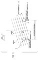
- FIG. 1 This basic sound source direction estimation scheme will be described with reference to Fig. 1 .
- Fig. 1 an environment is considered in which there is a single sound source 11, and two microphones 12 and 13 are installed at a spacing d. If the distance from each of the microphones 12 and 13 to the sound source 11 is sufficiently large relative to the microphone spacing d, sound waves can be approximated by plane waves, in which case it can be assumed that sound arrives at the two microphones at the same angle ⁇ .
- the angle ⁇ is defined with the direction orthogonal to the line connecting the two microphones (microphone-pair direction) taken as 0.
- the angle ⁇ is defined with the direction orthogonal to the line connecting the two microphones (microphone-pair direction) taken as 0.
- the difference in distance to the sound source between the two microphones can be represented as [d ⁇ cos ⁇ '].
- the angle [ ⁇ ] that determines the sound source direction can be computed in accordance with the above-mentioned equation.
- a description will be given of a method of computing the sound source direction by transforming observed signals into the time-frequency domain.
- X 1 ( ⁇ ,t) and X 2 ( ⁇ ,t) represent the results of applying a Short-time Fourier Transform (STFT) described later to a plurality of observed signals x 1 and x 2 , respectively, where ⁇ and t denote the frequency bin index and the frame index, respectively.
- STFT Short-time Fourier Transform
- the observed signals [x 1 , x 2 ] before undergoing the transform are referred to as time domain signals, and the signals [X 1 , X 2 ] after undergoing the short-time Fourier transform are referred to as time-frequency domain (or STFT domain) signals.
- hat( ⁇ ( ⁇ )) means that the angle ⁇ in the frequency bin ⁇ is a value estimated from an observed value. It should be noted that hat as used herein means symbol ( ⁇ ).
- Equation [1.4] mentioned above is for a given specific ⁇ (frequency bin index) and t (frame index), by calculating the sound source directions with respect to a plurality of ⁇ 's and t's and then taking the mean, a stable value of ⁇ can be obtained.
- n n>2 microphones, and calculate the sound source direction with respect to each of n(n+1)/2 pairs.
- Equations [1.5] to [1.7] below are equations for cases in which a plurality of microphones and a plurality of frames are used.
- Equation [1.5] A vector whose elements are the observed signals at individual microphones is defined as Equation [1.5], and the mean of the vector is defined by Equation [1.6].
- E t [ ] in this equation denotes the mean based on a frame in a given segment, and is defined by Equation [1.7]
- Equation [1.4] by using E t [X i ( ⁇ ,t)] and E t [X m ( ⁇ ,t)] in Equation [1.6] instead of X 1 ( ⁇ ,t) and X 2 ( ⁇ ,t), the mean of source direction corresponding to t0-th to t1-th frames, which is calculated from a pair of i-th microphone and m-th microphone, is found.
- the sound source direction can be computed in real-time (with a delay of less than one frame) and with high frequency (frame by frame).
- ICA Independent Component Analysis
- ICA refers to a type of multivariate analysis, and is a technique for separating multidimensional signals by exploiting statistical properties of the signals.
- ICA refers to, for example, "Introduction to the Independent Component Analysis” (Noboru Murata, Tokyo Denki University Press).
- ICA for sound signals, in particular, ICA in the time-frequency domain.
- a situation is considered in which different sounds are being played from N sound sources, and those sounds are observed at n microphones.
- the sounds (source signals) produced from the sound sources are subject to time lags, reflections, and so on before arriving at the microphones. Therefore, signals observed at a microphone j (observed signals) can be represented as an equation that sums up convolutions between source signals and transfer functions with respect to all sound sources as indicated by Equation [2.1] below.
- these mixtures will be referred to as "convolutive mixtures”.
- Equation [2.2] Observed signals for all microphones can be represented by a single equation as in Equation [2.2] below.
- x t A 0 ⁇ s t + ... + A L ⁇ s ⁇ t - L
- s t s 1 t ⁇ s N t
- x t x 1 t ⁇ x n t
- a l a 11 l ⁇ a 1 ⁇ N l ⁇ ⁇ ⁇ a n ⁇ 1 l ⁇ a nN l
- x(t) and s(t) are column vectors having x k (t) and s k (t) as elements, respectively.
- Equation [3.1] ⁇ is the frequency bin index and t is the frame index.
- Equation [3.5] for computing the separated results [Y] is prepared, and then a separating matrix W( ⁇ ) is determined such that the individual components of the separated results: Y( ⁇ ,t) are maximally independent.
- Equations [4.1] to [4.3] below are iterated until the separating matrix W( ⁇ ) converges (or a predetermined number of times).
- Equation [4.1] to [4.3] are performed with respect to all frequency bins, and further, Equation [4.1] is performed with respect to all the frames of charged observed signals.
- Equation [4.2] denotes the mean over all frames.
- the superscript H attached at the upper right of Y( ⁇ ,t) indicates the Hermitian transpose (taking the transpose of a vector or a matrix, and also transforming its elements into conjugate complex numbers).
- Equation [4.4] The separated results Y(t) are represented by Equation [4.4].
- ⁇ ⁇ (Y(t)) which denotes a vector in which elements of all the channels and all the frequency bins of the separated results are arranged, is represented by Equation [4.5].
- Each element ⁇ ⁇ (Y k (t)) is called a score function, and is a logarithmic derivative of the multidimensional (multivariate) probability density function (PDF) of Y k (t) (Equation [4.6]).
- PDF multidimensional probability density function
- Equation [4.7] a function represented by Equation [4.7] can be used, in which case the score function ⁇ ⁇ (Y k (t)) can be represented as Equation [4.9].
- Equation [4.8] ⁇ denotes a term for adjusting the scale of Y k ( ⁇ ,t), for which an appropriate positive constant, for example, sqrt(M) (square root of the number of frequency bins) is substituted.
- Equation [4.3] ⁇ is a positive small value (for example, about 0.1) called a learning ratio or learning coefficient. This is used for gradually reflecting ⁇ W( ⁇ ) calculated in Equation [4.2] on the separating matrix W( ⁇ ).
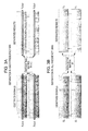
- Equation [4.1] represents separation in one frequency bin (see Fig. 3A ), it is also possible to represent separation in all frequency bins by a single equation (see Fig. 3B ).
- Equation [4.1] Equation [4.11]
- Equation [4.12] Equation [4.1] and Equation [4.11] are used selectively as necessary.
- spectrograms The diagrams of X 1 to X n and Y 1 to Y n shown in Figs. 3A and 3B are called spectrograms, in which the results of short-time Fourier transform (STFT) are arranged in the frequency bin direction and the frame direction.
- the vertical direction represents the frequency bin
- the horizontal direction represents the frame. While lower frequencies are drawn at the top in Equation [4.4] and Equation [4.11], lower frequencies are drawn at the bottom in the spectrograms.
- ICA is a type of Blind Source Separation (BSS), and has such characteristics that in the separation process, no knowledge about signal sources (the frequency distributions, the directions of arrival, and the like of sound sources) is necessary, and separation can be performed even without any prior knowledge about the sound velocity, microphone spacing, microphone gain, transfer function, and the like. Further, an assumption other than independence (for example, sparseness or the like) is also unnecessary, and separation is possible even when a plurality of sound sources keep playing and mixtures are occurring in the frequency domain (that is, even when the assumption of sparseness does not hold). These characteristics prove advantageous for the scheme that involves "sound source separation after direction estimation" described later.
- BSS Blind Source Separation
- a scheme for estimating the sound source direction by using ICA is described in, for example, Japanese Patent No. 3881367 .
- B ⁇ W ⁇ ⁇ - 1
- B ⁇ B 11 ⁇ ⁇ B 1 ⁇ n ⁇ ⁇ ⁇ ⁇ B n ⁇ 1 ⁇ ⁇ B nn ⁇
- the k-th column of an estimated transfer function matrix B( ⁇ ) as its inverse matrix B( ⁇ ) represents transfer functions (see Fig. 4B ) from the estimated sound sources Y k ( ⁇ ,t) to individual microphones.
- X mk ⁇ ⁇ t B mk ⁇ ⁇ Y k ⁇ ⁇ t
- the sound source direction can be computed by the same method as in the case of "1. Sound Source Estimation using Phase Difference between Microphones" described at the beginning of this specification.
- Equation [5.4] Equation [5.4] below is obtained.
- ⁇ ⁇ imk ⁇ asin ⁇ M - 1 ⁇ C ⁇ ⁇ ⁇ - 1 ⁇ d im F ⁇ angle B ik ⁇ ⁇ B mk ⁇
- d im denotes the distance between the i-th microphone and the m-th microphone.
- the above-described method of computing the sound source direction from the inverse matrix of a separating matrix of ICA has an advantage in that even when a plurality of sound sources are simultaneously playing, the directions of individual sound sources can be found.
- Equation [4.1] to Equation [4.3] are iterated until the separating matrix W( ⁇ ) converges (or a predetermined number of times), is performed in batch. That is, as described above, the iteration process of Equation [4.1] to Equation [4.3], in which Equation [4.1] to Equation [4.3] are iterated after charging the whole of observed signals, is referred to as learning.
- This batch process can be applied to real-time (low-delay) sound source separation through some contrivance.
- a description will be given of the configuration disclosed in "Japanese Patent Application No. 2006-331823 : REAL-TIME SOUND SOURCE SEPARATION APPARATUS AND METHOD", which is a patent application previously filed by the same inventor as the present application.
- the processing scheme disclosed in Japanese Patent Application No. 2006-331823 splits observed signal spectrograms into a plurality of overlapped blocks 1 to N, and learning is performed for each block to find a separating matrix.
- the reason why the blocks are overlapped is to achieve both the accuracy and the frequency of updates of the separating matrix.
- a separating matrix found from each block is applied to subsequent observed signals (not applied to the same block) to generate the separated results.
- staggered application Such a scheme will be referred to as "staggered application”.
- Fig. 6 illustrates the "staggered application".
- the separating matrix corresponding to the block containing the observed signals X(t) for example, an observed signal block 66 containing the current time
- the observed signals X(t) are multiplied by the separating matrix learned from a learning data block 61 that is a block preceding the block 66, thereby generating the separated results corresponding to X(t), that is, separated results Y(t)64 at the current time. It is assumed that the separating matrix learned from the learning data block 61 is already obtained at the point in time of the frame t.
- a separating matrix is considered to represent a process reverse to a mixing process.
- a process of obtaining a separating matrix from overlapped blocks can be executed, for example, on a general PC by a computation according to a predetermined program.
- the configuration disclosed in Japanese Patent Application No. 2006-331823 proposes a scheme in which a plurality of processing units called threads for finding a separating matrix from overlapped blocks are run in parallel at staggered times. This parallel processing scheme will be described with reference to Fig. 7 .
- Fig. 7 shows the transitions of processing over time of individual threads serving as the units of processing.
- Fig. 7 shows six threads, Threads 1 to 6. Each thread repeats three states of A) Charging, B) Learning, and C) Waiting. That is, the thread length corresponds to the total time length of the three processes of A) Charging, B) Learning, and C) Waiting. Time progresses from left to right in Fig. 7 .
- the "A) Charging" is the segment of dark gray in Fig. 7 .
- a thread charges observed signals.
- the overlapped blocks in Fig. 5 can be expressed by staggering the charging start times between threads. Since the charging start time is staggered by 1/4 of the charging time in Fig. 7 , assuming that the charging time in one thread is, for example, four seconds, the staggered time between threads equals one second.
- each thread transitions in state to "B) Learning".
- the "B) Learning” is the segment of light gray in Fig. 7 .
- Equations [4.1] and [4.3] described above are iterated with respect to the charged observed signals.
- the learning is ended, and the thread transitions to the "C) Waiting" state (the white segment in Fig. 7 ).
- the separating matrix W obtained by learning is used for performing separation until learning in the next thread is finished. That is, the separating matrix W is used as a separating matrix 63 shown in Fig. 6 .
- a description will be given of the separating matrix used in each of applied-separating-matrix specifying segments 71 to 73 along the progression of time shown at the bottom of Fig. 7 .
- an initial value for example, a unit matrix
- a separating matrix derived from an observed-signal charging segment 74 in Thread 1 is used as the separating matrix 63 shown in Fig. 6 .
- the numeral "1" shown in the segment 72 in Fig. 7 indicates that the separating matrix W used in this period is obtained through processing in Thread 1.
- the numerals on the right from the applied-separating-matrix specifying segment 72 also each indicate from which thread the corresponding separating matrix is derived.
- the separating matrix is used as the initial value of learning. This will be referred to as "inheritance of a separating matrix".
- the separating matrix 72 derived from Thread 1 is already obtained, so the separating matrix 72 is used as the initial value of learning.
- Permutation between threads refers to, for example, a problem such that in the separating matrix obtained in the first thread, speech is outputted on the first channel and music is outputted on the second channel, whereas the reverse is true for the separating matrix obtained in the second thread.
- permutation between threads can be reduced by performing "inheritance of a separating matrix" so that when a separating matrix that has been obtained in another thread exists, the separating matrix is used as the initial value of learning.
- the degree of convergence can be improved as the separating matrix is inherited by the next thread.
- the separating matrix is updated at an interval substantially equal to a shift between threads, that is, a block shift width 76.
- a delay in sound source direction estimation still remains as long as the direction is computed from a separating matrix. That is, in Fig. 6 , the separated results corresponding to the observed signals X(t) 62 at the current time are obtained by multiplying X(t) by the separating matrix 63. That is, as the separated results 64 at the current time in Fig. 6 , the following separated results are obtained.
- Y t WX t
- the sound source direction computed from the separating matrix 63 corresponds to the learning data block 61 that is a preceding segment.
- the sound source direction corresponding to the observed signals 62 at the current time is obtained at the point in time when a new separating matrix is learned from the block 66 containing the current time.
- the separated results strictly corresponding to the sound source direction computed from the separating matrix (63) are generated by multiplying the observed signals in the segment of the learning data block 61 used for learning of the separating matrix, by the separating matrix 63.
- multiplication between the separating matrix 63 and the observed signals in the learning data block 61 is not performed.
- tracking lag does not necessarily exert an adverse influence on the performance of sound source separation, even in that case, tracking lag sometimes exerts an adverse influence on the performance of direction estimation.
- tracking lag does not necessarily exert an adverse influence on the performance of sound source separation, even in that case, tracking lag sometimes exerts an adverse influence on the performance of direction estimation.
- Fig. 8 is a conceptual diagram of tracking lag.
- one sound source starts playing at given time (t) (for example, when someone suddenly starts talking).
- Other sound sources may either keep playing or remain silent before and after the time at which the sound source starts playing.
- the degree of convergence of learning is shown in (a) Graph 1.
- a separating matrix learned in the "inactive” segment is used for some time.
- a separating matrix learned in the "inactive” segment is used in a data segment 85b in (a) Graph 1 as well.
- the length of the data segment 85b is longer than the learning time (for example, the time length indicated at 77 in Fig. 7 ) and shorter or equal to the sum total of the block shift width (for example, the time length indicated at 76 in Fig. 7 ) and the learning time, and is determined by the balance between the timing at which learning starts and the timing at which a sound starts playing.
- a separating matrix learned from an observation segment including the "sound-source active" segment begins to be used.
- a data segment 85c of the convergence degree data in (a) Graph 1 the separating matrix learned from the observation segment 81b is used. It should be noted, however, that if the number of learning loops is set small (for example, if learning is aborted in 20 loops to shorten the learning time, even through learning converges in 100 loops), the separating matrix has not converged completely. Therefore, the degree of convergence in the data segment 85c in (a) Graph 1 is low.
- the separating matrix converges as the "inheritance of a separating matrix" (see “4. Real-time Implementation of ICA” described above) is repeated between threads. This occurs in the sequence of data segments 85c, 85d, 85e, and 85f of the convergence degree data in (a) Graph 1. It is assumed that the separating matrix has converged sufficiently in the data segment 85f and thereafter.
- the separating matrix has converged in a data segment 88b of the mismatch degree data, the degree of mismatch becomes high due to the reason (1). As the separating matrix gradually converges in data segments 88c to 88f, the degree of mismatch also decreases.
- the mismatch between a separating matrix and observed signals exerts an adverse influence.
- the data segment 88b shown in Fig. 8 if the "shifting of time point" described in "2. Tracking Lag" is performed, an inaccurate direction (direction computed not from the sound-source active segment but the sound-source inactive segment) is given.
- the separating matrix since the separating matrix has not converged yet in the data segments 88c and 88d, there is a possibility that a separating matrix calculated from those segments is also inaccurate.
- the sound source can be computed without tracking lag in the case of "1.
- Sound Source Estimation using Phase Difference between Microphones described above. That is, employing "Real-time ICA plus Sound Source Estimation from Separating Matrix" in an environment where there is only a single sound source presents more problems than "1. Sound Source Estimation using Phase Difference between Microphones".
- a unit matrix is substituted for the separating matrix (that is, a unit matrix is used in the segment 71 shown in Fig. 7 ). While an inverse matrix exists for a unit matrix (the unit matrix itself), all elements except the diagonal elements of the inverse matrix are 0. Thus, the sound source direction is not found from Equation [5.4] described above. Therefore, in the case of the scheme that finds the sound source direction from the inverse matrix of a separating matrix, the sound source direction is not found for the segment 71 in which a unit matrix is substituted for the separating matrix.
- the update frequency of direction and the corresponding segment coincide with the update frequency of the separating matrix and the learning data segment, and separate settings are not allowed. That is, the direction update interval substantially coincides with the block shift width 76 shown in Fig. 7 , and the direction thus obtained is the mean of observed signals within the block (for example, the data segment 71 shown in Fig. 7 ).
- the above-mentioned sound source direction estimation using ICA is a scheme which performs direction estimation after performing sound source separation (that is, ICA).
- ICA sound source separation
- the above-mentioned order is reversed, that is, after performing sound source direction estimation, the resulting value is used to perform sound source separation.
- a problem common to schemes that perform "sound source separation after direction estimation” is that the accuracy of direction estimation affects the separation accuracy. Further, even if the direction itself can be estimated correctly, there is a possibility that separation accuracy may decrease due to other factors at the point of sound source separation.
- the transfer function from the sound source of a target sound to each microphone it is necessary that the transfer function from the sound source of a target sound to each microphone be previously found.
- the transfer function is estimated from the direction and position of the sound source.
- the accuracy of separation decreases if such an assumption or values differ from those in the actual environment.
- ICA Independent Component Analysis
- cross-covariance matrices are calculated between observed signals and the separated results, and the sound source direction is computed from the phase differences between elements of the cross-covariance matrices.
- the proportionality factor between phase difference and frequency is estimated with good accuracy.
- the process configuration according to an embodiment of the present invention has the following advantages over the method according to the related art in which the sound source direction is estimated from the inverse matrix of a separating matrix. (1) Calculation can be performed with less delay than in the case of the separating matrix-based method. (2) Direction can be computed with the frequency of every single frame. (3) Direction can be computed even in cases where the inverse matrix of a separating matrix does not exist, and cases where 0 is included in the elements of the inverse matrix.
- a signal processing apparatus including: a learning processing unit that finds a separating matrix for separating mixed signals in which outputs from a plurality of sound sources are mixed, by a learning process that applies ICA (Independent Component Analysis) to observed signals including the mixed signals; a separation processing unit that applies the separating matrix to the observed signals to separate the mixed signals and generate separated signals corresponding to each of the sound sources; and a sound source direction estimating unit that computes a sound source direction of each of the separated signals generated in the separation processing unit, in which the sound source direction estimating unit calculates cross-covariance matrices between the observed signals and the separated signals in corresponding time segments in time-frequency domain, computes phase differences between elements of the cross-covariance matrices, and computes a sound source direction corresponding to each of the separated signals by applying the computed phase differences.
- ICA Independent Component Analysis
- the separation processing unit executes a short-time Fourier transform (STFT) on the mixed signals in which outputs from a plurality of sound sources are mixed, to generate observed signal spectrograms in time-frequency domain, and applies the separating matrix to the observed signal spectrograms to generate separated signal spectrograms in time-frequency domain
- the sound source direction estimating unit calculates cross-covariance matrices between the observed signal spectrograms and the separated signal spectrograms in corresponding time segments in time-frequency domain, computes phase differences between elements of the cross-covariance matrices, and compute a sound source direction corresponding to each of the separated signals by applying the computed phase differences.
- STFT short-time Fourier transform
- the sound source direction estimating unit computes covariance matrices of the observed signals in time-frequency domain, and computes the cross-covariance matrices between the observed signals and the separated signals by applying the computed cross-covariance matrices, and Hermitian transpose matrices of the separating matrices computed by the learning processing unit.
- the sound source direction estimating unit computes, in a process of computing the phase differences, phase differences corresponding to a pair of microphones that are signal input devices put at different positions, individually with respect to each of the sound sources (channels).
- the sound source direction estimating unit executes a straight-line fitting process which computes a proportionality constant (slope of a straight line) between a phase angle and a frequency, by using information on the phase differences between the elements of the cross-covariance matrices, and computes a sound source direction corresponding to each of the separated signals by using the proportionality constant.
- a proportionality constant slope of a straight line
- the sound source direction estimating unit computes the proportionality constant (slope of a straight line) by executing a recursive method as the straight-line fitting process, the recursive method including executing an unwrap process of correspondence information between the phase angle and the frequency in order from the lowest frequency to perform an updating process of the proportionality constant.
- the sound source direction estimating unit computes the proportionality constant (slope of a straight line) by executing a linear search method as the straight-line fitting process, the linear search method including gradually changing a value of the proportionality constant (slope of a straight line) from preset minimum to maximum values, calculating an error with respect to the information on the phase differences, and selecting a proportionality constant with small error.
- the sound source direction estimating unit computes the proportionality constant (slope of a straight line) by executing, as the straight-line fitting process, a linear search method that includes gradually changing a value of the proportionality constant (slope of a straight line) from preset minimum to maximum values, calculating an error with respect to the information on the phase differences, and selecting a proportionality constant with small error, and a recursive method that includes executing, by using the proportionality constant obtained by the linear search method as an initial value, an unwrap process of correspondence information between phase angle and frequency in order from the lowest frequency to perform an updating process of the proportionality constant.
- the sound source direction estimating unit computes a plurality of proportionality constants (slopes of straight lines) corresponding to each pair of microphones that are signal input devices put at different positions, selects pieces of data with small fitting error from the computed plurality of proportionality constants (slopes of straight lines), and computes a mean (average) of the selected pieces of data to compute a final value of the proportionality constant (slope of a straight line).
- the signal processing apparatus further executes, by using the proportionality constant (slope of a straight line) acquired as a result of the straight-line fitting process, frequency masking which suppresses a frequency component of signal separation results which has phase angle data that deviates largely from the straight line.
- proportionality constant slope of a straight line
- the signal processing apparatus further generates the separating matrix by using the proportionality constant (slope of a straight line) acquired as a result of the straight-line fitting process, and uses the generated separating matrix in the learning processing unit.
- the sound source direction estimating unit computes a matrix[P k ] generated by horizontally arranging vectors [p im ] connecting individual microphones within individual pairs of microphones after normalizing their length to 0, and a vector [D k ] generated by horizontally arranging path differences [D imk ] with respect to the individual pairs of microphones after normalization by microphone spacing, and computes an angle of a sound source direction, or a vector indicating a sound source direction as seen from each of the pairs of microphones, by applying the computed matrix [P k ] and the computed vector [D k ].
- a signal processing method which is executed in a signal processing apparatus, including the steps of: a learning processing unit finding a separating matrix for separating mixed signals in which outputs from a plurality of sound sources are mixed, by a learning process that applies ICA (Independent Component Analysis) to observed signals including the mixed signals; a separation processing unit applying the separating matrix to the observed signals to separate the mixed signals and generate separated signals corresponding to each of the sound sources; and a sound source direction estimating unit computing a sound source direction of each of the generated separated signals, in which the computing of a sound source direction includes calculating cross-covariance matrices between the observed signals and the separated signals in corresponding time segments in time-frequency domain, computing phase differences between elements of the cross-covariance matrices, and computing a sound source direction corresponding to each of the separated signals by applying the computed phase differences.
- ICA Independent Component Analysis
- a program for causing a signal processing apparatus to execute signal processing including the steps of: a learning processing unit finding a separating matrix for separating mixed signals in which outputs from a plurality of sound sources are mixed, by a learning process that applies ICA (Independent Component Analysis) to observed signals including the mixed signals; a separation processing unit applying the separating matrix to the observed signals to separate the mixed signals and generate separated signals corresponding to each of the sound sources; and a sound source direction estimating unit computing a sound source direction of each of the generated separated signals, in which the computing of a sound source direction includes calculating cross-covariance matrices between the observed signals and the separated signals in corresponding time segments in time-frequency domain, computing phase differences between elements of the cross-covariance matrices, and computing a sound source direction corresponding to each of the separated signals by applying the computed phase differences.
- ICA Independent Component Analysis
- a separating matrix for separating mixed signals in which outputs from a plurality of sound sources are mixed is found by a learning process that applies Independent Component Analysis (ICA) to observed signals including the mixed signals, the separating matrix is applied to the observed signals to generate separated signals, and a sound source direction estimating process of computing the sound source direction of each separated signal is executed.
- ICA Independent Component Analysis
- cross-covariance matrices are calculated between the observed signals and the separated signals in corresponding time segments in time-frequency domain, the phase differences are computed between elements of the cross-covariance matrices, and the sound source direction corresponding to each of the separated signals is computed by applying the computed phase differences.
- a proportionality constant slope of a straight line
- the sound source direction corresponding to each of the separated signals is computed by using the proportionality constant.
- the program according to an embodiment of the present invention is a program that can be provided to a general-purpose system capable of executing a variety of program codes, via a recording medium or communication medium that is provided in a computer-readable format.
- a program in a computer-readable format, processes corresponding to the program are realized on the computer system.
- system refers to a logical assembly of a plurality of devices, and is not limited to one in which the constituent devices are located within the same housing.
- signals in which a plurality of signals are mixed are separated by using Independent Component Analysis (ICA) to estimate the sound source direction.
- ICA Independent Component Analysis
- cross-covariance matrices are calculated between observed signals and the separated results, and the sound source direction is calculated by using the cross-covariance matrices instead of a separating matrix.
- FIG. 9 is a diagram in which novel features according to an embodiment of the present invention are added to Fig. 6 described above.
- a segment containing the current time is set in both (a) observed signals and (b) separated results.
- the current frame index be [t]
- the start time of the segment be the [t - L + 1]-th frame
- the end time be the [t]-th frame.
- Data of the segment containing the current time includes observed signal data 92 on the observed signal side, and separated result data 94 on the separated result side.
- Et[ ] denotes the mean over the segment. Specifically, Et[ ] is calculated by Equation [6.2].
- ⁇ X ( ⁇ ) and ⁇ Y ( ⁇ ) denote the means of X( ⁇ ,t) and Y( ⁇ ,t) over the segments, and are calculated by Equation [6.3] and Equation [6.4], respectively.
- the operation of subtracting ⁇ X ( ⁇ ) and ⁇ Y ( ⁇ ) can be omitted in cases where the mean of the signals can be expected to be close to 0.
- a sound source direction estimating unit of the signal processing apparatus calculates cross-covariance matrices between observed signal spectrograms and separated signal spectrograms in corresponding time segments in the time-frequency domain.
- the sound source direction can be obtained by using the cross-covariance matrices ⁇ XY ( ⁇ ) calculated in this way in the same manner as the separating matrix W( ⁇ ).
- the sound source direction estimated from the cross-covariance matrices ⁇ XY ( ⁇ ) combines the characteristics of that obtained by the separating matrix and that obtained by the [A1. Sound Source Direction Estimation using Phase Difference between Microphones] described above.
- a description will be given in this regard.
- Equation [6.5] the right-hand side of Equation [6.5] can be transformed as Equation [6.8], that is, into a form in which the inverse matrix of the separating matrix is multiplied by the covariance matrices of the separated results themselves.
- Equation [6.8] represents a transformation for illustrative purpose, and it is not necessary to calculate the inverse matrix in the actual processing.
- Equation [7.1] the sound source direction is estimated by Equation [7.2] (similarly to Equation [5.4]). That is, estimation of the sound source direction is possible even without using an inverse matrix.
- the above-described cross-covariance matrices can be also considered as the products of the covariance matrices of observed signals and the Hermitian transpose of the separating matrix.
- the separating matrix is a unit matrix. This corresponds to a state with signals are least separated (observed signals are outputted as they are).
- Equation [7.2] is the same in value as the sound source direction computed from each of Equation [1.6] and Equation [1.4] ("A1. Sound Source Direction Estimation using Phase Difference between Microphones"). That is, the covariance matrices ⁇ XY ( ⁇ ) of observed signals have n ⁇ n elements, and the respective elements can be represented as in Equation [6.7] (the mean is subtracted as necessary). While ⁇ XY ( ⁇ ) has n columns, substantially the same value as that obtained by using Equation [1.6] is computed no matter which column is used.
- the sound source direction computed from cross-covariance matrices takes the same value as the sound source direction computed from the inverse matrix of a separating matrix.
- the sound source direction computed from the cross-covariance matrices takes the same value as the sound source direction computed from the phase differences between microphones. That is, the sound source direction computed from the cross-covariance matrices combines the characteristics of both the cases.
- the scheme using cross-covariance matrices has the following advantages:
- Calculation of covariance matrices can be performed by calculating Equation [6.10] or Equation [6.11] for computing the cross-covariance matrices ⁇ XY ( ⁇ ) mentioned above every time the frame index t increases (as necessary, the mean is subtracted from X( ⁇ ,t) and Y( ⁇ ,t)).
- the complexity of this calculation is small in comparison to calculation of an inverse matrix.
- the complexity is constant even if the length L (see Fig. 9 ) of a segment set in the separated result spectrograms shown in Fig. 9 is increased. Therefore, in the method according to an embodiment of the present invention, the sound source direction can be computed with frame-by-frame frequency and with low delay.
- the segment used for computation of the sound source direction (each of the segment 92 set in the observed signal spectrograms and the segment 94 set in the separated result spectrograms shown in Fig. 9 ) can be set separately from the segment used for learning of the separating matrix (for example, the learning data block segment 91). Therefore, an optimum length that provides both trackability and stability may be set.
- Equations [6.2], [6.10], and [6.11] mentioned above which are equations for computing the covariance matrices, even if the coefficient 1/(L - 1) is omitted, the same value is computed as the sound source direction.
- correlation matrices Equation [6.12], where ⁇ ik ( ⁇ ) denotes individual elements of the covariance matrices and represented by Equation [7.1]
- the same sound source direction is computed.
- Equation [6.13] the second term on the right-hand side of Equation [6.13] is a matrix whose off-diagonal elements are 0, and its diagonal elements h 1 ..., h n represent arbitrary complex numbers.
- Equation [7.2] sound source directions can be estimated for individual frequency bins and individual microphone pairs, and those sound source directions are averaged to find the sound source direction.
- the method of averaging the values computed in individual frequency bins has the following problems.
- a technique called "straight-line fitting” is employed. This is a scheme in which a plot of phase difference against frequency bin index ⁇ is approximated by a straight line, and the sound source direction is estimated from the slope of the straight line.
- a description will be given of the principle and method involved.
- Equation [8.1] a value obtained by taking the ratio between elements in the i-th and m-th rows, followed by normalizing the magnitude a complex number to 1, is defined as r imk ( ⁇ ).
- r imk ( ⁇ ) is represented by Equation [8.1] below.
- sign(z) represents an operation of normalizing the magnitude of a complex number z to 1, and is defined by Equation [8.2].
- the expression "element ratio between a and b" as used in the following description is taken to represent both.
- the same value is computed no matter which is performed first. For example, in the expression in the middle of Equation [8.1], the same value is obtained when the ratio is calculated after taking the sign with respect to the numerator and the denominator, or when the sign is calculated after taking the ratio.
- Equation [r imk ( ⁇ )] can be approximated by Equation [8.3] above. That is, the phase angle of r imk ( ⁇ ) has proportionality with [ ⁇ - 1], and the relationship of Equation [8.4] holds between its proportionality constant K imk and the sound source direction.
- the plotted phase angle (r imk ( ⁇ )) of r imk ( ⁇ ) is approximated by a straight line, the slope of the straight line is K imk , and if K imk is found, then the sound source direction for each microphone pair is also found.
- Figs. 10A and 10B show a specific example.
- Figs. 10A and 10B are diagrams illustrating the plotted data of phase angle angle (r imk ( ⁇ )) of data r imk ( ⁇ ) obtained by taking the ratio between an element in the i-th row and an element in the m-th row of the k-th column of cross-covariance matrices and further normalizing its magnitude to 1, and acquisition of the slope [K imk ] of a straight line obtained by a straight-line approximation process and a sound source direction computing process for each microphone pair.
- r imk phase angle angle
- Fig. 10A shows a plot of phase angle with respect to r imk ( ⁇ ) calculated from real data, in which the vertical axis indicates the frequency bin ⁇ , and the horizontal axis indicates the phase angle. It can be seen that points are aligned in a substantially straight line. However, since the value of phase angle angle( ) can be identified only within a range of 2 ⁇ (in this drawing, - ⁇ to ⁇ ), "jumps" of values exist between - ⁇ and ⁇ .
- Fig. 10B shows the result of straight-line fitting performed by taking the "jumps" into account.
- an unwrap operation of adding 2N ⁇ (N is an appropriate integer) to the values of phase angle was executed for each frequency bin. This process was executed respect to an unwrap processing region 103 shown in Fig. 10B . This operation is referred to as "unwrap”. After this unwrap, the best fitting straight line through the points, that is, a fitting straight line 104 shown in Fig. 10B is found. The specific algorithm for this process will be described later.
- the proportionality coefficient K imk can be estimated also by using the complex number r imk ( ⁇ ) directly, instead of using the phase angle of r imk ( ⁇ ). This method will be described with reference to Figs. 11A to 11D . In the following description, this method will be also referred to as "straight-line fitting".
- Figs. 11A and 11B show plotted data of real and imaginary parts of r imk ( ⁇ ), respectively. It can be seen that curves close to cosine and sine are drawn respectively. The approximation of these plots by exp(jK iml ( ⁇ - 1)) in Equation [8.3] mentioned above yields a proportionality constant for finding K imk corresponding to the best-fitting curves for both the real and imaginary parts (a curve 105 shown in Fig. 11C and a curve 106 shown in Fig. 11D ).
- an error between r imk ( ⁇ ) and exp(jK iml ( ⁇ - 1)) is defined by Equation [8.5], and the value of K imk that minimizes this error may be found. (See Equation [8.6].
- arg min indicates an operation of finding the value of K imk that makes the value inside brackets minimum.)
- Equation [8.5] a fitting error
- the configuration of a signal processing apparatus according to an embodiment of the present invention is shown in Fig. 12 .
- the apparatus configuration shown in Fig. 12 is based on Japanese Patent Application No. 2006-331823 "REAL-TIME SOUND SOURCE SEPARATION APPARATUS AND METHOD" previously filed by the present applicant.
- a sound source direction estimating unit 125 is added to the configuration disclosed in Japanese Patent Application No. 2006-331823 .
- the signal processing apparatus shown in Fig. 12 can be specifically implemented by, for example, a PC. That is, respective processes in a separation processing unit 123, a learning processing unit 110, the sound source direction estimating unit, and a subsequent-stage processing unit 124 can be executed by, for example, a CPU that executes processes according to a pre-defined program.
- the separation processing unit 123 shown at the center of Fig. 12 mainly performs separation of observed signals.
- the learning processing unit 110 shown on the right-hand side of Fig. 12 performs learning of a separating matrix.
- the process in the separation processing unit 123, and the process in the learning processing unit 110 are performed in parallel.
- the process in the separation processing unit 123 is a foreground process, and the process in the learning processing unit 110 is a background process.
- the separation processing unit 123 performs an operation of applying a separating matrix to audio signals inputted from an AD conversion unit 122 to generate the separated results, and also replacing the separating matrix with the latest one in accordance with the progress of processing in the learning processing unit 110.
- the sound source direction estimating unit 125 In the sound source direction estimating unit 125, observed signals and separated results (or the relationship of Equation [6.5]) are inputted from the separation processing unit 123, and the sound source direction is computed from the observed signals and the separating matrix.
- Sound recorded by a plurality of microphones 121 are converted into digital data in the AD conversion unit 122, and then sent to a Fourier transform unit 126 of the separation processing unit 123.
- the digital data is transformed into frequency-domain data by a windowed short-time Fourier transform (details of which will be given later).
- a predetermined number of pieces of data called frames are generated. Subsequent processes are performed in these frame units.
- the Fourier transformed data is sent to each of the sound source direction estimating unit 125, a separating unit 127, and a thread control unit 112 of the learning processing unit 110.
- the separated results Y(t) are sent to an inverse Fourier transform unit 128 and the sound source direction estimating unit 125.
- a separating matrix may be sent to the sound source direction estimating unit 125 instead of the separated results.
- the separated results [Y(t)] sent to the inverse Fourier transform unit 128 are transformed into time domain signals, and sent to the
- subsequent-stage processing unit a 124a that executes processing at subsequent stages.
- processing at subsequent stages include sound recognition and speaker recognition.
- frequency-domain data can be used as it is, in which case an inverse Fourier transform can be omitted.
- observed signals sent to the thread control unit 112 of the learning processing unit 110 are sent to a thread computation unit 111 that performs computations using a plurality of learning threads 111-1 to 111-N.
- the thread computation unit 111 finds a separating matrix from the observed signals by using ICA batch processing. The separating matrix thus found is sent to the separating unit 127 of the separation processing unit 123 via the thread control unit 112.
- observed signals sent to the sound source direction estimating unit 125 are used for calculation of cross-covariance matrices together with the separated results generated in the separating unit 127 (or together with a separating matrix). Therefore, the sound source direction is calculated. (Details will be given later.)
- the sound source direction thus found is sent to a subsequent-stage processing unit b 124b that executes processing at subsequent stages.
- Examples of processing at subsequent stages executed by the subsequent-stage processing unit b 124b include a process called diarization. That is, when combined with the results of sound recognition, speaker recognition, and the like, a set of information indicating "who made what speech at what time and from what direction (at what position)" can be generated.
- Fig. 13 is a configuration diagram for a case in which cross-covariance matrices are calculated from observed signals and the separated results (Equation [6.1])
- Fig. 14 is a configuration diagram for a case in which cross-covariance matrices are calculated from observed signals and a separating matrix (Equation [6.5]).
- Inputs to the sound source direction estimating unit 125 shown in Fig. 13 are:
- the one frame of observed signals X(t) supplied from the Fourier transform unit 126 is stored into an observed signal buffer 133.
- the observed signal buffer 133 is a ring buffer with a length L, and inputs from the (L + 1)-th input onwards are written over the oldest signal within the buffer. For example, although inputs from X(0) up to X(L - 1) are stored into the observed signal buffer 133 as they are, at the time of storing X(L), X(L) is written over the area of X(0). Of course, as necessary, all of the past observed signals may be saved.
- the one frame of separated results Y(t) supplied from the separating unit 127 is stored into a separated result buffer 134.
- the separated result buffer 134 is a ring buffer with the length L.
- a computing unit 132 calculates cross-covariance matrices for each frequency bin from L frames of observed signals and separated results, and stores the results into a cross-covariance matrix buffer 135. As described above with reference to Fig. 9 , the computing unit 132 calculates cross-covariance matrices between corresponding time segments of observed signal spectrograms and separated result spectrograms in the time-frequency domain, and stores the results into the cross-covariance matrix buffer 135.
- the computing unit 132 calculates element ratios and phase differences for individual channels and microphone pairs (such as r imk ( ⁇ ) in Equation [8.1] and ⁇ imk ( ⁇ ) in Equation [8.9]), and stores the calculated results into a phase difference buffer 136.
- the computing unit 132 finds a proportionality constant (slope of a straight line) K imk that best fits the phase differences stored in the phase difference buffer 136, stores the results into a straight-line slope buffer 137, and also stores a fitting error err imk into a fitting error buffer 138.
- the computing unit 132 calculates a sound source direction [ ⁇ k ] from the proportionality constant (slope of a straight line) stored in the straight-line slope buffer 137 and the fitting error err imk , and stores the sound source direction [ ⁇ k ] as the calculated results into a sound source direction buffer 139.
- Respective computations in the sound source direction estimating unit 125 are performed in the computing unit 132. Although omitted in this drawing, the computing unit 132 are connected to the individual buffers in this drawing so as to allow data exchange.
- the one frame of observed signals X(t) supplied from the Fourier transform unit 126 is stored into an observed signal buffer 143. This corresponds to the observed signal data segment 92 that is a segment containing the current time on the observed signal side shown in Fig. 9 .
- the observed signal buffer 143 is a ring buffer with a length L.
- the computing unit 142 calculates not cross-covariance matrices but covariance matrices of observed signals themselves, and stores the results into a covariance matrix buffer 144.
- the computing unit 142 receives an input of the separating matrix W that is being used in the separating unit 127 shown in Fig. 12 at the same time, calculates cross-covariance matrices [ ⁇ XY ] on the basis of Equation [6.5] described above, from the Hermitian transpose of this separating matrix and the covariance matrices stored in the covariance matrix buffer 144, and stores the calculated cross-covariance matrices into a cross-covariance matrix buffer 145.
- the computing unit 142 calculates element ratios and phase differences for individual channels and microphone pairs (such as r imk ( ⁇ ) in Equation [8.1] and ⁇ imk ( ⁇ ) in Equation [8.9]), and stores the calculated results into a phase difference buffer 146.
- the computing unit 142 finds a proportionality constant (slope of a straight line) K imk that best fits the phase differences stored in the phase difference buffer 146, stores the results into a straight-line slope buffer 147, and also stores a fitting error err imk into a fitting error buffer 148.
- the computing unit 142 calculates a sound source direction [ ⁇ k ] from the proportionality constant (slope of a straight line) stored in the straight-line slope buffer 147 and the fitting error err imk , and stores the sound source direction [ ⁇ k ] as the calculated results into a sound source direction buffer 149.
- the configuration shown in Fig. 14 proves advantages in terms of saving of buffer memory in comparison to the configuration shown in Fig. 13 , since it is unnecessary to store L frames of signals with respect to the separated results.
- a current-frame-index holding counter 151 is incremented by 1 every time one frame of observed signals is supplied, and is returned to the initial value upon reaching a predetermined value.
- the incrementing of the counter may be synchronized with the sample index of time domain signal, instead of being synchronized with the frame index.
- a learning-initial-value holding unit 152 holds the initial value of separating matrix W when executing a learning process in each thread.
- the initial value of separating matrix W is basically the same as that of the latest separating matrix, a different value may be used as well.
- a separating matrix to which rescaling (a process of adjusting power between frequency bins, details of which will be given later) has not been applied is used as the learning initial value
- a separating matrix to which rescaling has been applied is used as the latest separating matrix.
- a planned-charging-start-timing-specifying-information holding unit 153 holds information used for keeping the timing of starting charging at a constant interval between a plurality of threads.
- the planned charging start timing may be expressed using relative time, or may be managed by the frame index or by the sample index of time domain signal instead of relative time. The same applies to information for managing other kinds of "timing".
- An observed-signal-charging-timing-information holding unit 154 holds information indicating on the basis of observed signals acquired at what timing the separating matrix X being currently used in the separating unit 127 is learned, that is, the relative time or frame index of observed signals corresponding to the latest separating matrix. Although both the charging start and charging end timings of corresponding observed signals may be stored in the observed-signal-charging-timing-information holding unit 154, if the block length, that is, if the charging time of the observed signals is constant, it suffices to save only one of these timings.
- the thread control unit 112 has a pointer holding unit 155 that holds pointers linked to individual threads, and controls the plurality of threads 111-1 to 111-N by using the pointer holding unit 115.
- Each of the threads 111-1 to 111-N executes batch ICA by using the functions of the respective modules of an observed signal buffer 161, a separated result buffer 162, a learning computation unit 163, and a separating-matrix holding unit 164.
- the observed signal buffer 161 holds observed signals supplied from the thread control unit 112, and its capacity is equal to or larger than the capacity of observed signals corresponding to one block length. It should be noted, however, that if "frame thinning-out on observed signals" described later is to be performed, the size of the buffer may be reduced by an amount corresponding to the amount of thinning.
- the separated result buffer 162 holds the separated results prior to separating-matrix convergence, which are computed by the learning computation unit 163.
- the learning computation unit 163 executes a process of separating observed signals charged in the observed signal buffer 161, on the basis of a separating matrix W used for separation process which is held in the separating-matrix holding unit 164, charging the separated results into the separated-result buffer 162, and also updating the separating matrix being learned by using the separated results charged in the separated-result buffer 162.
- a thread is a state transition machine, and the current state is stored in a state storage unit 165.
- the state of a thread is controlled by the thread control unit 112 on the basis of the counter value of a counter 166.
- the counter 166 changes in value in synchronization with supply of one frame of observed signals, and switches its state on the basis of this value. Details in this regard will be given later.
- An observed-signal start/end timing holding unit 167 holds at least one of pieces of information indicating the start timing and the end timing of observed signals used for learning.
- information indicating timing may be the frame index or sample index, or may be relative time information.
- both the start timing and the end timing may be stored, if the block length, that is, if the charging time of the observed signals is constant, it suffices to save only one of these timings.
- a learning end flag 168 is a flag used for notifying the thread control unit 112 of the end of learning. During activation of a thread, the learning end flag 168 is set OFF (flag is not up), and at the point when learning ends, the learning end flag 168 is set ON. Then, after the thread control unit 112 recognizes that learning has ended, the learning end flag 168 is set OFF again through control of the thread control unit 112.
- a pre-processing data holding unit 169 is an area that saves data that becomes necessary when observed signals to which pre-processing has been applied are returned to the original state. Specifically, for example, in cases where normalization of observed signals (adjusting the variance to 1 and the mean to 0) is executed in pre-processing, since values such as a variance (or a standard deviation or its inverse) and a mean are held in the pre-processing data holding unit 169, original signals prior to normalization can be recovered by using these values. In cases where, for example, uncorrelation (also referred to as pre-whitening) is executed as pre-processing, a matrix by which the observed signals are multiplied during the uncorrelation is held.
- uncorrelation also referred to as pre-whitening
- Values held in the state storage unit 165, the counter 166, and the observed-signal start/end timing holding unit 167 can be rewritten from an external module such as the thread control unit 112. For example, even while a learning process loop is being run in this thread, the thread control unit 112 can change the value of the counter 166.
- specifications may be such that each of the threads 111-1 to 111-N spontaneously changes its state on the basis of the value of the counter 166 of the thread itself, or specifications may be such that the thread control unit 112 issues a command instructing "transition to a specified state" (hereinafter, referred to as "state transition command") to the corresponding thread in accordance with the value of the counter 166 or the value of the learning end flag 168, and each thread transitions in state in response to the supplied command.
- state transition command instructing "transition to a specified state”
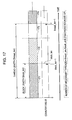
- Fig. 17 shows one of the threads described above with reference to Fig. 7 .
- observed signals for the duration of a specified time that is, one block length are charged into the buffer. After the elapse of the specified time, the state transitions to learning.
- a learning process loop is executed until the separating matrix W converges (or a predetermined number of times), and a separating matrix corresponding to the observed signals charged in the charging state is found. After the separating matrix converges (or after the learning process loop is executed a predetermined number of times), the state transitions to waiting.
- a thread length (thread_len) as the total time width of the "charging” state, the "learning” state, and the “waiting” state is set, and basically, the time from when the "learning" state ends to the end of the thread length is set as the "waiting" state time (wait time). After the wait time elapses, the state returns to the "charging" state of observed signals.
- While these times may be managed in units of milliseconds or the like, the times may be measured in units of frames that are generated by a short-time Fourier transform. In the following description, it is assumed that these times are measured (for example, counted up) in units of frames.
- Thread 1 is a thread that has transitioned to "charging”
- the other threads are threads that have transitioned to "waiting”.
- block_len The time necessary for charging observed signals is referred to as block length (block_len) (see Fig. 17 ).
- thread_len the time necessary for the one cycle of charging, learning, and waiting is referred to as thread length (thread_len). While these times may be managed in units of millimeters or the like, frames generated by a short-time Fourier transform may serve as units of management. In the following description, frames serve as units.
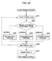
- the state transitions from "charging to learning” and "waiting to charging” are made on the basis of the counter value. That is, within a thread that has started from “charging” (a charging state 171 in Fig. 17 and a charging state 183 in Fig. 18 ), the counter is incremented by 1 every time one frame of observed signals is supplied, and when the value of the counter becomes equal to the block length (block_len), the state is made to transition to "learning" (a learning state 172 in Fig. 17 and a learning state 184 in Fig. 18 ). Although learning is performed in the background in parallel with the separating process, during this learning as well, the counter is incremented by 1 in synchronization with the frame of observed signals.
- the state is made to transition to "waiting" (a waiting state 173 in Fig. 17 and a waiting state 182 in Fig. 18 ).
- the counter is incremented by 1 in synchronization with the frame of observed signals. Then, when the counter value becomes equal to the thread length (thread_len), the state is made to transition from "charging” (the charging state 171 in Fig. 17 and the charging state 183 in Fig. 18 ), and the counter is returned to 0 (or an appropriate initial value).
- the counter is set to a value corresponding to the time for which the thread is to be put in wait state.
- Thread 2 in Fig. 7 transitions to "charging” after waiting for a time equal to the block shift width (block_shift).
- Thread 3 is made to wait for a time equal to twice the block shift width (block_shift ⁇ 2).
- the counter of Thread 2 is set as: thread length ⁇ block shift width : thread_len ⁇ block_shift .
- the counter of Thread 3 is set as: thread length ⁇ 2 ⁇ block shift : thread_len ⁇ block_shift ⁇ 2 .
- the number of learning threads to be prepared is determined by the thread length and the block shift width. Letting the thread length be represented as thread_len, and the block shift width be represented as block_shift, the number of necessary learning threads is found by thread length / block shift width , that is, thread_length / block_shift .
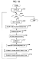
- the process in the sound source direction estimating unit 125 and the "foreground process (separation)" in the separation processing unit 123 can be both performed in synchronization with frames. Accordingly, the two processes will be collectively described with reference to the flowchart shown in Fig. 19 .
- step S101 Upon start-up of the system, in step S101, various kinds of initialization are performed. Details of the initialization will be described later.
- the process from the sound input in step S103 to the transmission in step S110 is repeated until processing on the system ends (Yes in step S102).
- the sound input in step S103 is a process of capturing a predetermined number of samples from an audio device (or a network, a file, or the like depending on the embodiment) (this process will be referred to as "capture"), and charging the captured samples in a buffer. This is performed for the number of microphones.
- the captured data will be referred to as observed signal.
- step S104 the observed signal is sliced off for each predetermined length, and a short-time Fourier transform (STFT) is performed. Details of the short-time Fourier transform will be described with reference to Fig. 20 .
- STFT short-time Fourier transform
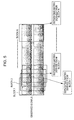
- an observed signal x k recorded with the k-th microphone in the environment as shown in Fig. 2 is shown in Fig. 20(a) .
- a window function such as a Hanning window or a sine window is applied to frames 191 to 193, which are sliced data each obtained by slicing a predetermined length from the observed signal x k .
- the sliced units are referred to as frames.
- a discrete Fourier transform a Fourier transform on a finite segment, abbreviated as DFT
- FFT fast Fourier transform
- the frames to be sliced may be overlapped, like the frames 191 to 193 shown in the drawing, which makes it possible for the spectrums X k (t-1) to X k (t+1) of consecutive frames to change smoothly.
- Spectrums laid side by side in accordance with the frame index are referred to as spectrograms.
- Fig. 20(b) shows an example of spectrograms.
- the Fourier transform is also performed for the number of channels.
- the Fourier transformed results for all channels and for one frame are represented by a vector X(t) (Equation [4.11] described above).
- step S104 after the observed signal is sliced into each predetermined length, and a short-time Fourier transform (STFT) is performed, in step S105, control is performed with respect to each learning thread. Details in this regard will be given later.
- STFT short-time Fourier transform
- step S107 an inverse Fourier transform (inverse FT) is applied to the separated results Y(t), thereby recovering the signals back to time domain signals. Thereafter, in step S108, the separated results are transmitted to subsequent-stage processing.
- inverse FT inverse Fourier transform
- step S109 the sound source direction is updated by using one frame of observed signals and separated results (or by using one frame of observed signals and the latest separating matrix). Details in this regard will be given later.
- step S110 the sound source direction thus found is transmitted to subsequent-stage processing. Steps S103 to S110 mentioned above are repeated until the end.
- step S101 in the flowchart shown in Fig. 19 Details of the initialization process in step S101 in the flowchart shown in Fig. 19 will be described with reference to the flowchart in Fig. 21 .
- step S151 the thread control unit 112 shown in Figs. 12 and 15 initializes itself. Specifically, in the thread control unit 112, the current-frame-index holding counter 151 (see Fig. 15 ) is initialized to 0, and an appropriate initial value is substituted into the learning-initial-value holding unit 152 (see Fig. 15 ).
- the initial value may be a unit matrix, or if the separating matrix W at the last system termination is saved, the separating matrix W at the last system termination, or an appropriately transformed version of this separating matrix may be used.
- an initial value may be computed and set on the basis of the sound source direction.
- a value of (number of necessary threads - 1) ⁇ [block shift width (block_shift)] is set in the planned-charging-start-timing-specifying-information holding unit 153. This value indicates the timing (frame index) at which charging in a thread with the largest thread index starts. Then, since timing information (frame index or relative time information) indicating observed signals corresponding to the latest separating matrix is held in the observed-signal-charging-timing-information holding unit 154, initialization is performed at this time, and 0 is held.
- the initial value to be held in the separating-matrix holding unit 113 may be a unit matrix, or if the separating matrix W at the last system termination is saved, the separating matrix W at the last system termination, or an appropriately transformed version of this separating matrix may be used.
- an initial value may be computed and set on the basis of the sound source direction.
- step S152 the thread control unit 112 secures the number i of necessary threads to be executed in the thread computation unit 111, and sets their state to the "initial" state.
- the number i of necessary threads is found by rounding up the fractional part of thread length/block shift width (thread_len/block_shift) (that is, an integer larger than and closest to the value of thread_length/block_shift).
- step S153 the thread control unit 112 starts a thread control loop, and until initialization of all threads is finished, the thread control unit 112 detects uninitialized threads and executes the processes from step S154 to step S159.
- step S154 the thread control unit 112 determines whether or not the thread index is 1.
- step S155 the thread control unit 112 controls a thread with a thread index 1 (for example, the thread 111-1), and initializes its counter 166 (see Fig. 16 ) (for example, sets the counter 166 to 0).
- a thread index 1 for example, the thread 111-1
- initializes its counter 166 for example, sets the counter 166 to 0.
- step S156 the thread control unit 112 issues to the thread with the thread index 1 (for example, the thread 111-1) a state transition command for causing the state to transition to the "charging" state, and the process proceeds to step S159.
- the thread index 1 for example, the thread 111-1
- step S157 the thread control unit 112 sets the value of the counter 166 of the corresponding thread (one of the threads 111-2 to 111-i) to thread_len - block_shift ⁇ (thread index - 1).
- step S158 the thread control unit 112 issues a state transition command for causing the state to transition to the "waiting" state.
- step S159 the thread control unit 112 initializes information within the thread which has not been initialized yet, that is, information indicating a state stored in the state storage unit 165 (see Fig. 16 ), and information other than the counter value of the counter 166. Specifically, for example, the thread control unit 112 sets the learning end flag 168 (see Fig. 16 ) OFF, and initializes values in the observed-signal start/end timing holding unit 167 and the pre-processing data holding unit 169 (for example, set the values to 0).
- step S160 the thread loop is ended, and the initialization ends.
- the thread control unit 112 initializes all of the plurality of threads secured in the thread computation unit 111.
- step S153 to step S160 is repeated for the number i of launched threads
- parallel processes equal to the number i of threads may be executed.
- parallel processes may be executed instead of repeating the process loop.
- step S154 to S158 in Fig. 21 correspond to the "initialization" process at the beginning, and the transmission of a state transition command immediately after the initialization process in the sequence diagram shown in Fig. 22.
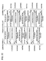
- Fig. 22 shows a sequence of control performed by the thread control unit 112 with respect to the plurality of Learning Threads 1 and 2. Each thread repeatedly executes the process of waiting, charging, and learning. After the thread control unit provides observed signals to each thread, and each thread charges observed data, a learning process is performed to generate a separating matrix, and the separating matrix is provided to the thread control unit.
- this flowchart represents a flow as seen from the thread control unit 112, and not from the learning threads 111-1 to 111-N.
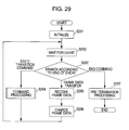
- “learning-state process” indicates a process performed by the thread control unit 112 when the state of a learning thread is "learning” (for the process of the learning thread itself, reference should be made to Fig. 30 ).
- Steps S201 to S206 represent a loop with respect to a learning thread, and the loop is run for the number of threads generated in step S152 of the flow shown in Fig. 21 (parallel processes may be performed as well).
- step S202 the current state of the learning thread is read from the state storage unit 165 (see Fig. 16 ), and one of "waiting-state process”, “charging-state process”, and “learning-state process” is executed in accordance with the read value. Details of the respective processes will be described later in detail.
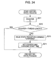
- step S202 the thread control unit 112 acquires information indicating the internal state of a thread having a thread index indicated by the variable "s", which is held in the state storage unit 165 for the thread. If it is detected that the state of the thread having a thread index indicated by the variable "s" is "waiting”, in step S203, the thread control unit 112 executes a waiting-state process, which will be described later with reference to the flowchart in Fig. 24 , and the process proceeds to step S206.
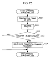
- step S204 If it is detected in step S202 that the state of the thread having a thread index indicated by the variable "s" is "charging”, in step S204, the thread control unit 112 executes a charging-state process, which will be described later with reference to the flowchart in Fig. 25 , and the process proceeds to step S206.
- step S205 the thread control unit 112 executes a learning-state process, which will be described later with reference to the flowchart in Fig. 26 .
- step S207 the thread control unit 112 increments the frame index held in the current-frame-index holding counter 151 (see Fig. 15 ) by 1, and ends the thread control process.
- the thread control unit 112 can control all of the plurality of threads in accordance with their state.
- This waiting-state process is a process that is executed by the thread control unit 112 when the state of a thread corresponding to the variable "s" is "waiting" in the thread control process described above with reference to Fig. 23 .
- step S211 the thread control unit 112 increments the counter 166 (see Fig. 16 ) of the corresponding thread 111 by 1.
- step S212 the thread control unit 112 determines whether or not the value of the counter 166 of the corresponding thread 111 is smaller than the thread length (thread_len). If it is determined in step S212 that the value of the counter 166 is smaller than the thread length, the waiting-state process is ended, and the process proceeds to step S206 in Fig. 23 .
- step S212 If it is determined in step S212 that the value of the counter 166 is not smaller than the thread length, in step S213, the thread control unit 112 issues to the corresponding thread 111 a state transition command for causing the state of the thread 111 to transition to the "charging" state.
- the thread control unit 112 issues a state transition command for causing a thread, which is in the "waiting" state in the state transition diagram described above with reference to Fig. 18 , to "charging".
- step S214 the thread control unit 112 initializes the counter 166 (see Fig. 16 ) (for example, sets the counter 166 to 0) of the corresponding thread 111, and sets, in the observed-signal start/end timing holding unit 167 (see Fig. 16 ), observed-signal charging start timing information, that is, the current frame index held in the current-frame-index holding counter 151 (see Fig. 15 ) of the thread control unit 112, or equivalent relative time information or the like. Then, the thread control unit 112 ends the waiting-state process, and proceeds to step S206 in Fig. 23 .
- the thread control unit 112 ends the waiting-state process, and proceeds to step S206 in Fig. 23 .
- the thread control unit 112 can control a thread that is in the "waiting" state, and on the basis of the value of the counter 166 of the thread, cause the state of the thread to transition to "charging".
- This charging-state process is a process that is executed by the thread control unit 112 when the state of a thread corresponding to the variable "s" is "charging" in the thread control process described above with reference to Fig. 23 .
- step S221 the thread control unit 112 supplies one frame of observed frames X(t) to the corresponding thread 111 for learning. This process corresponding to the supply of observed signals from the thread control unit to the respective threads.
- step S222 the thread control unit 112 increments the counter 166 of the corresponding thread 111 by 1.
- step S223 the thread control unit 112 determines whether or not the value of the counter 166 of the corresponding thread 111 is smaller than the block length (block_len), in other words, whether or not the observed signal buffer 161 (see Fig. 16 ) of the corresponding thread is full. If it is determined in step S223 that the value of the counter 166 of the corresponding thread 111 is smaller than the block length, in other words, the observed signal buffer 161 of the corresponding thread is not full, the charging-state process is ended, and the process proceeds to step S206 in Fig. 23 .
- block_len block length
- step S224 the thread control unit 112 issues to the corresponding thread 111 a state transition command for causing the state of the thread 111 to transition to the "learning" state, ends the charging-state process, and proceeds to step S206 in Fig. 23 .
- the thread control unit 112 issues a state transition command for causing a thread, which is in the "charging” state in the state transition diagram described above with reference to Fig. 18 , to "learning".
- the thread control unit 112 can supply observed signals to a thread that is in the "charging” state to control the charging of the observed signals, and on the basis of the value of the counter 166 of the thread, cause the state of the thread to transition from "charging” to "learning".
- This learning-state process is a process that is executed by the thread control unit 112 when the state of a thread corresponding to the variable "s" is "learning” in the thread control process described above with reference to Fig. 23 .
- step S231 the thread control unit 112 determines whether or not the learning end flag 168 (see Fig. 16 ) of the corresponding thread 111 is ON. If it is determined in step S231 that the learning end flag is ON, the process proceeds to step S237 described later.
- step S231 If it is determined in step S231 that the learning end flag is not ON, that is, a learning process is being executed in the corresponding thread, the process proceeds to step S232 where a process of comparing times is performed.
- the "comparing of times” refers to a process of comparing the observed-signal start time 167 (see Fig. 16 ) recorded within the learning thread 111, with the charging start time 154 (see Fig. 15 ) corresponding to the current separating matrix which is saved in the thread control unit 112. If the observed-signal start time 167 (see Fig. 16 ) recorded in the thread 111 is earlier than the charging start time 154 corresponding to the current separating matrix which is saved in the thread control unit 112, the subsequent processes are skipped.
- step S233 the thread control unit 112 increments the counter 166 of the corresponding thread 111 by 1.
- step S234 the thread control unit 112 determines whether or not the value of the counter 166 of the corresponding thread 111 is smaller than the thread length (thread_len). If it is determined in step S234 that the value of the counter 166 is smaller than the thread length, the thread control unit 112 ends the learning-state process, and proceeds to step S206 in Fig. 23 .
- step S235 the thread control unit 112 subtracts a predetermined value from the value of the counter 166, ends the learning-state process, and proceeds to step S206 in Fig. 23 .
- a case where the value of the counter reaches the thread length during learning corresponds to a case where learning takes such a long time that the period of "waiting" state does not exist. In that case, since learning is still being continued, and the observed signal buffer 161 is being used, it is not possible to start the next charging. Accordingly, until learning ends, the thread control unit 112 postpones the start of the next charging, that is, issuing of a state transition command for causing the state to transition to the "charging" state. Thus, the thread control unit 112 subtracts a predetermined value from the value of the counter 166. While the value to be subtracted may be, for example, 1, the value may be larger than 1, for example, a value such as 10% of the thread length.
- the wait times in other threads may be adjusted so that the interval of the charging start timing becomes regular again. This process is executed in step S241. Details of this wait-time adjusting process will be described later.
- step S231 A description will be given of the process in a case when the learning end flag is determined to be ON in step S231. This process is executed once every time a learning loop within a learning thread ends. If it is determined in step S231 that the learning end flag is ON, and a learning process has ended in the corresponding thread, in step S237, the thread control unit 112 sets the learning end flag 168 of the corresponding thread 111 OFF. This process represents an operation for preventing this branch from being continuously executed.
- the thread control unit 112 checks whether or not an abort flag 170 (see Fig. 16 ) of the thread is ON or OFF. If the abort flag 170 is ON, the thread control unit 112 performs a separating-matrix updating process in step S239, and performs a wait-time setting process in step S241. On the other hand, if the abort flag 170 (see Fig. 16 ) of the thread is OFF, the separating-matrix updating process in step S239 is omitted, and the wait-time setting process is performed in step S241. Details of the separating-matrix updating process in step S239, and the wait-time setting process in step S241 will be described later.
- the thread control unit 112 can determine whether or not learning has ended in a thread in the "learning” state by referring to the learning end flag 168 of the corresponding thread. If the learning has ended, the thread control unit 112 updates the separating matrix W and sets the wait time, and also causes the state of the thread to transition from "learning" to "waiting” or “charging".
- step S251 the thread control unit 112 determines whether or not the start timing of observed signals held in the observed-signal start/end timing holding unit 167 (see Fig. 16 ) of the thread is earlier than the charging start timing corresponding to the current separating matrix, which is held in the observed-signal-charging-timing-information holding unit 154 (see Fig. 15 ).
- a learning segment 77 ends earlier than a learning segment 78.
- cases may occur in which the learning segment 78 ends earlier than the learning segment 77.
- step S251 if the determination in step S251 is not executed, and a separating matrix derived from the thread in which learning has ended later is treated as the latest separating matrix, a separating matrix W2 derived from Thread 2 is overwritten by a separating matrix W1 derived from Thread 1 which is obtained by learning with observed signals acquired at the earlier timing. Accordingly, to ensure that a separating matrix obtained with observed signals acquired at the later timing is treated as the latest separating matrix, the start timing of observed signals held in the observed-signal start/end timing holding unit 167 is compared with the charging start timing corresponding to the current separating matrix which is held in the observed-signal-charging-timing-information holding unit 154.
- step S201 If it is determined in step S201 that the start timing of observed signals is earlier than the charging start timing corresponding to the current separating matrix, in other words, if it is determined that the separating matrix W obtained as a result of learning in this thread has been learned on the basis of signals observed at an earlier timing than those corresponding to the separating matrix W being currently held in the observed-signal-charging-timing-information holding unit 154, the separating matrix obtained as a result of learning in this thread is not used, and thus the separating-matrix updating process ends.
- step S251 If it is determined in step S251 that the start timing of observed signals is not earlier than the charging start timing corresponding to the current separating matrix, that is, if it is determined that the separating matrix W obtained as a result of learning in this thread has been learned on the basis of signals observed at a later timing than those corresponding to the separating matrix W being currently held in the observed-signal-charging-timing-information holding unit 154, in step S252, the thread control unit 112 acquires the separating matrix W obtained by learning in the corresponding thread, and supplies the separating matrix W to the separating-matrix holding unit 113 (see Fig. 12 ) and sets the separating matrix W.
- step S253 the thread control unit 112 sets the initial value of learning in each of threads held in the learning-initial-value holding unit 152.
- the thread control unit 112 may set a separating matrix W obtained by learning in the corresponding thread, or may set a value different from a separating matrix W which is computed by using the separating matrix W obtained by learning in the corresponding thread.
- the value obtained after rescaling is applied (value obtained after "post-processing" in step S320 in the flow in Fig. 32 described later) is substituted into the separating-matrix holding unit 113 (see Fig. 12 ), and the value prior to the application of rescaling is substituted into the learning-initial-value holding unit 152.
- Other examples will be described in the section of modifications later.
- step S254 the thread control unit 112 sets timing information held in the observed-signal start/end timing holding unit 167 (see Fig. 16 ) of the corresponding thread, in the charging-timing-information holding unit 154 (see Fig. 15 ), and ends the separating-matrix updating process.
- step S254 an indication is provided regarding from observed signals in what time segment the separating matrix W being currently used, that is, the separating matrix W held in the separating-matrix holding unit 113 has been learned.
- a separating matrix obtained from observed signals acquired at the later timing is set as the latest separating matrix.
- step S281 the thread control unit 112 calculates the remaining wait time.
- Ct represent the planned charging start timing (frame index or corresponding relative time) held in the planned-charging-start-timing-specifying-information holding unit 153 (see Fig. 15 )
- Ft represent the current frame index held in the current-frame-index holding counter 151
- block_shift represent the block shift width.
- step S282 the thread control unit 112 determines whether or not the calculated remaining wait time rest is a positive value. If it is determined in step S282 that the calculated remaining wait time rest is not a positive value, that is, the calculated value is zero or a negative value, the process proceeds to step S286 described later.
- step S282 If it is determined in step S282 that the calculated remaining wait time rest is a positive value, in step S283, the thread control unit 112 issues to the corresponding thread a state transition command for causing the state of the thread to transition to the "waiting" state.
- step S284 the thread control unit 112 sets the value of the counter 166 (see Fig. 16 ) of the corresponding thread to thread_len-rest. Thus, the "waiting" state is continued until the value of the counter reaches thread-len.
- step S285 the thread control unit 112 adds the value of block_shift to the value Ct held in the planned-charging-start-timing-specifying-information holding unit 153 (see Fig. 15 ), that is, sets the value of Ct + block_shift as the next charging start timing in the planned-charging-start-timing-specifying-information holding unit 153, and ends the remaining-wait-time calculating process.
- step S282 If it is determined in step S282 that the calculated remaining wait time rest is not a positive value, that is, the calculated value is zero or a negative value, this means that charging has not started even through the planned charging start timing is passed, so it is necessary to start charging immediately. Accordingly, in step S286, the thread control unit 112 issues to the corresponding thread a state transition command for causing the state of the thread to transition to the "charging" state.
- step S287 the thread control unit 112 initializes the value of the counter (for example, sets the counter to 0).
- step S288 the thread control unit 112 sets the next charging start timing, that is, Ft indicating the current frame index, in the charging-start-timing-specifying-information holding unit 153, and ends the remaining-wait-time calculating process.
- the thread control unit and each learning thread operate in parallel, and the learning thread is run on the basis of a flowchart different from that for the thread control unit.
- processing in the learning thread will be described with reference to the flowchart in Fig. 29 .
- the thread 111 is initialized in step S291. Then, in step S292, the thread 111 waits until an event occurs (blocks processing). (This "wait” is different from “waiting” which indicates one state of a learning thread). The event occurs when one of the following actions has been performed.
- the subsequent processing is branched in accordance with which event has occurred (step S293). That is, in accordance with the event inputted from the thread control unit 112, the subsequent process is branched.
- step S293 If it is determined in step S293 that a state transition command has been inputted, the corresponding command processing is executed in step S294.
- step S295 If it is determined in step S293 that an input of a frame data transfer event has been received, in step S295, the thread 111 acquires transfer data. Next, in step S296, the thread 111 charges the acquired frame data in the observed signal buffer 161 (see Fig. 16 ), returns to step S292, and waits for the next event.
- the observed signal buffer 161 (see Fig. 16 ) has an array or stack structure, and observed signals are to be stored in a location of the same index as the counter.
- step S297 the thread 111 executes, for example, appropriate pre-termination processing such as freeing of the memory, and the process is ended.
- processing is executed in each thread on the basis of control by the thread control unit 112.
- step S301 in accordance with a supplied state transition command, the thread 111 braches the subsequent processing.
- a command instructing "transition to the XX state” will be expressed as “state transition command "XX"”.
- step S301 the supplied state transition command is a "state transition command "waiting”” that instructs transition to the "waiting” state
- step S302 the thread 111 stores information indicating that the current state is "waiting" into the state storage unit 165 (see Fig. 16 ), that is, transitions in state to "waiting", and ends the command processing.
- step S301 the supplied state transition command is a "state transition command "charging”” that instructs transition to the "charging” state
- step S303 the thread 111 stores information indicating that the current state is “charging” into the state storage unit 165, that is, transitions in state to "charging”, and ends the command processing.
- step S301 the supplied state transition command is a "state transition command "learning”” that instructs transition to the "learning” state
- step S304 the thread 111 stores information indicating that the current state is "learning” into the state storage unit 165, that is, transitions in state to "learning”.
- step S305 the thread 111 executes a separating-matrix learning process. Details of this process will be given later.
- step S306 to notify the thread control unit 112 of the end of learning, the thread 111 sets the learning end flag 168 ON and ends the process. By setting the flag, the thread 111 notifies the thread control unit 112 to the effect that learning has just ended.
- the state of each thread is made to transition on the basis of a state transition command supplied from the thread control unit 112.
- step S311 as necessary, the learning computation unit 163 (see Fig. 16 ) of the thread 111 executes pre-processing on observed signals charged in the observed signal buffer 161.
- Equation [9.2] is a relational expression of X', the separating matrix W, and the separated results Y.
- Equation [9.3] The equations from Equation [9.3] and below will be described during description of a rescaling process in the post-processing in step S320 described later.
- step S312 the learning computation unit 163 acquires, as the initial value of a separating matrix, a learning initial value W held in the learning-initial-value holding unit 152 of the thread control unit 112, from the thread control unit 112.
- the processes from steps S313 to S319 represent a learning loop, and these processes are repeated until W converges or until the abort flag becomes ON.
- the abort flag is a flag that is set ON in step S236 in the flow of the learning-state process in Fig. 26 described above. The abort flag becomes ON when a learning started later ends earlier than a learning started earlier. If it is determined in step S313 that the abort flag is ON, the process is ended.
- step S313 If it is determined in step S313 that the abort flag is OFF, the process proceeds to step S314.
- step S314 If it is determined in step S314 that the value of the separating matrix W has converged, the process proceeds to step S320 described later, where post-processing is executed, and the process is ended. That is, the learning process loop is executed until the separating matrix W converges.
- step S314 If it is determined in step S314 that the value of the separating matrix W has not converged (or if the number of times the loop is executed has not reached a predetermined value), the processing proceeds into the learning loop in steps S315 to S319. Learning is performed as a process of iterating Equations [4.1] to [4.3] described above for all frequency bins. That is, to find the separating matrix W, Equations [4.1] to [4.3] are iterated until the separating matrix W converges (or a predetermined number of times). This iteration is referred to as "learning".
- the separated results Y(t) are represented by Equation [4.4]
- Equations [4.1] to [4.3] are to be computed for each frequency bin, by running a loop with respect to frequency bins in steps S315 and S319, ⁇ W is found for all frequency bins.
- step S313 the process returns to step S313 to perform the determination with regard to the abort flag, and the determination of the convergence of the separating matrix in step S314.
- the process is ended if the abort flag is ON. If convergence of the separating matrix is confirmed in step S314 (or a specified number of loops has been reached), the process proceeds to step S320.
- step S320 the following processes are executed as post-processing.
- the separating matrix W found by the above-described processes (steps S315 to S319 in Fig. 31 ) is not equivalent to that obtained by separating the observed signals X prior to normalization, but is a separating matrix obtained by separating the observed signals X' obtained after normalization. Accordingly, the separating matrix W found by the above-described processes is corrected so as to be transformed into one equivalent to that obtained by separating the observed signals X prior to normalization. Specifically, by using the matrix S applied at the time of normalization, a correction may be performed such that W ⁇ WS.
- the balance (scale) between frequency bins of the separated results Y differs from the expected one of the source signals in some cases.
- the scale of frequency bins is corrected in post-processing. Thus correction is referred to as rescaling.
- Rescaling is performed by finding a correction matrix R, which is contained in Equation [9.3] indicated as an expanded form of Equation [9.1] described above with reference to the pre-processing (step S311) such as normalization on the observed signals X, by using Equation [9.6], and then multiplying the separating matrix W by the correction matrix R (diag( ⁇ ) in Equation [9.6] denotes a diagonal matrix with a given vector on its diagonal). That is, W ⁇ RW is performed.
- ⁇ k ( ⁇ ) in Equation [9.6] is a value that makes the value in brackets of [arg min] on the right-hand side of Equation [9.4] minimum, which is specifically calculated by Equation [9.5].
- E t [] denotes the mean over all frames within the block.
- Equation [4.2] is used as an equation based on the natural gradient method
- Equation [4.13] representing a learning rule based on an algorithm called "Equi-variant Adaptive Separation via Independence” (EASI).
- An equation of EASI algorithm has a form that combines the gradient method and uncorrelation, and characteristically, converges faster than Equation [4.2] that is based on the natural gradient method.
- EASI Equi-variant Adaptive Separation via Independence
- Equation [4.14] the complexity can be reduced by the following equation transformations.
- E t [Y( ⁇ ,t)Y( ⁇ ,t) H ] as the first term can be transformed as Equation [4.14].
- E t [X( ⁇ ,t)X( ⁇ ,t) H ] in Equation [4.14] is calculated only once in the beginning (for example, calculated in step S311) since it is constant within the loop, and within the loop, it suffices to perform only an operation of multiplying E t [X( ⁇ ,t)X( ⁇ ,t) H ] from left and right with W( ⁇ ) and W( ⁇ ) H .
- Equation [4.15] the third term E t [Y( ⁇ ,t) ⁇ (Y(t)) H ] can be transformed as Equation [4.15]. This indicates that the third term can be also obtained by performing the Hermitian transpose after calculating the second term.
- 2 ] 1 holds for orthogonal elements of E t [Y( ⁇ ,t)Y( ⁇ ,t) H ], and 0 for other elements.
- 2 ] 1 holds for orthogonal elements of E t [Y( ⁇ ,t)Y( ⁇ ,t) H ], and 0 for other elements.
- Equation [4.16] is performed with respect to Y( ⁇ ,t)
- Equation [4.17] is performed with respect to W( ⁇ ).
- diag( ) denotes an orthogonal matrix with its diagonal components given in parentheses.
- a process is performed in which, in a segment containing the current time, cross-covariance matrices are calculated between observed signals and the separated results, and the sound source direction is calculated by using the cross-covariance matrices instead of a separating matrix.
- the cross-covariance matrices ⁇ XY ( ⁇ ) are represented by Equation [6.1] described above.
- the flowchart shown in Fig. 32 corresponds to the process in Fig. 13 described above. That is, the flowchart represents a process flow in a case when cross-covariance matrices are calculated from the observed signals X and the separated results Y (Equation [6.1]).
- the flowchart shown in Fig. 33 corresponds to the process in Fig. 14 described above. That is, the flowchart represents a process flow in a case when cross-covariance matrices are calculated from observed signals X and the separating matrix W (Equation [6.5]).
- step S322 observed signals X(t) are stored into the observed signal buffer 133 (see Fig. 13 ). At that time, X(t) is written over an area in which X(t-L) has been stored.
- step S323 likewise, the separated results are stored into the separated result buffer 134.
- steps S324 to S326 may be performed on a frame by frame basis, depending on the intended application, the frequency of performing these processes may be once every several frames.
- the sound source direction estimating process is ended.
- phase difference calculation in step S324 is a process of generating the plot shown in Figs. 10A and 10B with respect to all channels and all microphone pairs. Details of this process will be given later.
- the straight-line fitting process in step S325 is a process of finding the best fitting straight line while unwrapping the phase angle at each point, with respect to the plot shown in Figs. 10A and 10B , for example.
- the straight-line fitting process is also a process of finding the best fitting cosine and sine curves with respect to the plot. Details of this process will be given later.
- straight lines shown in Fig. 41 are obtained from the plots of phase angle shown in Fig. 35 .
- each straight line obtained as a result of straight-line fitting is indicated by a dotted line.
- each straight line is depicted as extending off the left and right or the top and bottom of the plot diagram.
- step S327 the sound source direction for each sound source is calculated from hat(K imk ). Details of this process will be also given later.
- FIG. 33 represent a scheme for calculating cross-covariance matrices from the covariance matrices of observed signals and the Hermitian transpose of a separating matrix. This process corresponds to the configuration in Fig. 14 described above.
- step S332 observed signals X(t) are stored into the observed signal buffer 143 (see Fig. 14 ). At that time, X(t) is written over an area in which X(t-L) has been stored.
- steps S334 to S336 may be performed on a frame by frame basis, depending on the intended application, the frequency of performing these processes may be once every several frames.
- the sound source direction estimating process is ended.
- step S324 in the flowchart in Fig. 32
- step S334 in the flowchart in Fig. 33 .
- step S341 an area for storing the results is secured as necessary.
- Steps S342 to S348 represent a loop with respect to frequency bin. While varying the frequency bin ⁇ from 1 to M, steps S343 to S347 are repeated. (It should be noted, however, that when the system used is capable of parallel processing, parallel processing may be performed. The same applies to the channel loops or microphone pair loops in the following description).
- Steps S343 to S347 represent a loop with respect to channels (estimated sound sources, that is, separated results). For example, if there are four channels, the loop is repeated for all the channels from channel-1 to channel-4.
- the ratio between the elements ⁇ ik ( ⁇ ) and ⁇ mk ( ⁇ ) of the cross-covariance matrices ⁇ XY is calculated by Equation [8.1] described above, and the calculated element ratio is stored into the area secured in step S341.
- the phase angle of the element ratio is also calculated in accordance with Equation [8.9].
- the microphone pair loop is performed with respect to all microphone combinations in the flowchart in Figs. 34A and 34B
- the microphone pair loop may be performed only with respect to limited microphone pairs.
- phase difference described in this flow is, for example, a process of generating the plot shown in Figs. 10A and 10B with respect to all channels and all microphone pairs. For example, if the number of microphones is four, and the number of channels is four, then, as a result of the processing of the flow shown in Figs. 34A and 34B , data shown in Fig. 35 is generated.
- Fig. 35 represents 24 diagrams in which plots for Channels 1 to 4 as a plurality of estimated sound sources with respect to six combinations of two microphones (Microphones 1 and 2, 1 and 3, 1 and 4, 2 and 3, 2 and 4, and 3 and 4) selected from four microphones, Microphones 1 to 4, are set.
- phase angle is plotted with respect to r imk ( ⁇ ) calculated from cross-covariance matrices.
- the vertical axis indicates the frequency bin ⁇ , and the horizontal axis indicates the phase angle. Points are aligned substantially linearly.
- the phase angle angle( ) can be identified only within a range of 2 ⁇ (in this drawing, - ⁇ to ⁇ ), "jumps" of values exist between - ⁇ and ⁇ .
- step S325 in the flowchart in Fig. 32 a detailed description will be given of the "straight-line fitting" in step S325 in the flowchart in Fig. 32 , and step S335 in the flowchart in Fig. 33 .
- the flowchart shown in Fig. 36 is a schematic representation, and indicates that the fitting process in step S364 with respect to a single plot (for example, a single piece of plot data 351 shown in Fig. 35 ) is performed with respect to all microphone pairs (corresponding to the vertical direction in Fig. 35 ) in steps S363 to S365, and further with respect to all channels (corresponding to the horizontal direction in Fig. 35 ) in steps S362 to S366.
- a single plot for example, a single piece of plot data 351 shown in Fig. 35
- the recursive method is a scheme in which a slope K imk is found while unwrapping the phase angle ⁇ imk ( ⁇ ) expressed by Equation [8.9] mentioned above, in order from low frequency bins. Details of the recursion will be described with reference to Figs. 37 and 38 .
- Fig. 37 is a flowchart illustrating the sequence of a (straight-line) fitting process performed by the recursive method.
- K imk is a variable that stores not only the final slope but also a mid-process value of slope.
- step S371 an appropriate initial value is substituted into the slope K imk in advance.
- the initial value may be 0, which corresponds to a vertically oriented straight line in the case of Figs. 10A and 10B and Fig. 35 . If a slope obtained in the previous frame is saved, the slope may be used as well.
- Steps S373 to S375 are a recursive process. That is, in a state with the value of K imk (value in the mid-processing stage) found by using phase angles in frequency bins 2 to m - 1, the value of K imk is updated while unwrapping the phase angle in the ⁇ -th frequency bin.
- Step S373 means that a straight-line fitted through frequency bins 2 to m - 1 (straight-line 401 in Fig. 38 ) is extended to the ⁇ -th frequency bin (point P402 in Fig. 38 ).
- the point to which the straight line is extended is indicated by an uppercase character P, and its phase angle is indicated by a lowercase character p.
- the unwrap in step S374 is a transform process from Fig. 10A to Fig. 10B described above with reference to Figs. 10A and 10B . That is, the unwrap is a process of adding 2N ⁇ (N is an integer) to the phase angle ⁇ imk ( ⁇ ) at the frequency bin ⁇ so that the phase angle becomes maximally close to the point P. Specifically, the operation of Equation [10.2] may be performed after finding the value of N that satisfies Equation [10.1] below.
- phase angle ⁇ imk ( ⁇ ) prior to unwrapping is indicated as a point[ ⁇ imk ( ⁇ ) (old)] 403
- phase angle after unwrapping is indicated as a point[ ⁇ imk ( ⁇ ) (new)] 404.
- step S375 the slope K imk is updated while reflecting the value of the phase angle ⁇ imk ( ⁇ ) obtained after unwrapping (straight line 405 in Fig. 38 ).
- ⁇ imk the phase angle obtained after unwrapping
- Equation [10.4] is obtained. Since the loop of sigma (total sum) is unnecessary in the implementation of Equation [10.4], the complexity of Equation [10.4]is less than that of Equation [10.3].
- Equation [10.3] and Equation [10.4] have a characteristic in that the value of K imk varies greatly when ⁇ is small, and K imk varies less as ⁇ becomes larger. Therefore, the initial value substituted in step S371 is not much reflected on the final value of K imk .
- Equation [10.5] is used instead of Equation [10.4].
- ⁇ is a value larger than 1. The larger the value of ⁇ , the less is the variation of the slope K imk from the initial value.
- the frequency bin loop may be aborted mid-process, in which case a corresponding reduction in complexity can be achieved. For example, in situations where it is clear that sound sources are all human speech, the loop may be run only within a frequency range corresponding to the frequency band of speech.
- step S377 the fitting error is calculated in accordance with Equation [8.5] mentioned above. This value is used for the sound source direction calculation in step S336 in the flow of Fig. 33 mentioned above or the like.
- the recursive method has the following advantages.
- a fitting error is calculated by Equation [8.5] mentioned above while gradually varying the value of the slope K imk from a minimum value K min set in step S391 to a preset maximum value K max , and the value of the slope K imk that makes the error minimum and that minimum value are found.
- K max as the maximum value of the slope setting range is found by Equation [11.1] below.
- K max ⁇ ⁇ d M - 1 ⁇ F C
- ⁇ K (see step S386) which is the increment of K imk is a relatively small positive value.
- step S382 it is checked whether or not K exceeds the maximum value (K max ), and the process is ended if K exceeds the maximum value. If K does not exceed the maximum value (K max ) in step S382, in step S383, a fitting error err detected at a set angle is computed. The fitting error is calculated by Equation [8.5] mentioned above.
- step S384 the computed fitting error err and the fitting error err imk that is held are compared against each other, and if the calculated fitting error err is larger than the held fitting error err imk , the process proceeds to step S386, and the angle is updated.
- step S385 If the calculated fitting error err is not larger than the held fitting error err imk , the process proceeds to step S385, where the angle K imk as a variable is updated by the verified angle K, and the fitting error err imk is updated by the computed error err. Thereafter, the process proceeds to step S386, and the verified angle is updated. Further, the processes from step S382 onwards are repeated with respect to the updated angle K.
- step S364 of the flow in Fig. 36 is roughly divided into two steps. First, the linear search described above with reference to Fig. 39 is performed, and then the recursion shown in the flow in Fig. 37 is performed by using the slope K imk found by the linear search as the initial value.
- the recursion shown in the flow in Fig. 37 is performed by using the slope K imk found by the linear search as the initial value.
- this hybrid method differs from executing the linear search method and the recursive method independently.
- Equation [12.1] floor ⁇ d ⁇ F C + 1 2
- floor( ) denotes dropping of decimals (flooring). Since dropping is done after adding 1/2, this is equivalent to rounding off the decimals of dF/C.
- the increment of slope [ ⁇ K] to be employed in step S396 in Fig. 39 is calculated by Equation [12.3] mentioned above. That is, the optimum value is searched for among 2N+1 kinds of slope including - ⁇ N/(M - 1), - ⁇ (N - 1)/(M - 1), ..., 0, ..., ⁇ (N - 1)/(M - 1), and ⁇ N/(M - 1).
- the 2N+1 kinds of slope to be set correspond to respective straight lines 411 to 417 shown in Fig. 40 .
- Equation [10.1] is an integer, even if the value of the slope K imk changes within the range of ⁇ /( ⁇ - 1), the value of N becomes the same, and the same unwrapped results are obtained.
- step S371 shown in Fig. 37 by setting the optimum value found from among the 2N+1 kinds of slope mentioned above as the initial value [K imk ], the processes from step S372 onwards are executed.
- Equation [10.5] is used instead of Equation [10.3] and Equation [10.4] that are the computing equations for the slope [K imk ] mentioned above. It should be noted, however, that as the value of ⁇ in Equation [10.5], a value roughly equal to the number M of frequency bins is used. Alternatively, Equation [12.4] mentioned above may be used as well.
- Fig. 41 shows the results of straight-line fitting performed by using the plot data shown in Fig. 35 described above.
- Fig. 41 shows the results of straight-line fitting with respect to 24 diagrams, in which plots for Channels 1 to 4 as a plurality of estimated sound sources with respect to six combinations of two microphones (Microphones 1 and 2, 1 and 3, 1 and 4, 2 and 3, 2 and 4, and 3 and 4) selected from four microphones, Microphones 1 to 4, are set.
- Each plot is obtained by plotting phase angle with respect to r imk ( ⁇ ) calculated from cross-covariance matrices.
- the vertical axis indicates the frequency bin ⁇ , and the horizontal axis indicates the phase angle.
- each straight line obtained as a result of straight-line fitting is indicated by a dotted line. In the drawing, for clearly indicating the straight lines, each straight line is depicted as extending off the left and right or the top and bottom of the plot diagram.
- the flowchart shown in Fig. 42 represents a process of summing up the values of the slope K imk found for individual microphone pairs to compute the sound source direction ⁇ k . It should be noted, however, that the process is so designed that values obtained with respect to output channels not corresponding to any sound source, or with respect to microphone pairs in which straight-line fitting has failed are not reflected on the sound source direction.
- signals not corresponding to any sound source are outputted to some of output channels. (Specifically, sounds with only reverberation components are outputted.) Such output channels are easily distinguishable since the plot of phase angle does not lie on a straight line.
- Fig. 41 described above as showing the results of straight-line fitting shows plots and straight-line fitting results generated in the case where the number of microphones is four, and the number of channels (number of estimated sound sources) is four.
- the plot data for Channel 3 contains many points that deviate from straight lines. This data indicates that this estimated sound source (Channel 3) does not actually exist. That is, this indicates that the results correspond to the case where the number of simultaneous sound sources is three.
- this column of channel-3 represents an output not corresponding to any sound source. Since it is meaningless to calculate the sound source direction for such an output channel, it is necessary to detect and discard such a channel. Also, if straight-line fitting has failed only with respect to a specific channel, a more accurate value should be obtained by removing the pair and then finding the mean of sound source directions.
- Steps S401 to S410 in the calculation process flow for sound source direction shown in Fig. 42 represent a channel loop, and indicates that the following process is performed with respect to each column (channel) in Fig. 41 , for example.
- step S402 initial values are substituted into the following variables that store results:
- Steps S403 to S406 represent a microphone pair loop, and this means that processing is performed with respect to the six phase angle plots in each column of Fig. 41 . That is, sound source directions are calculated from the respective six plots, and the calculated values are averaged.
- the fitting error err imk in step S404 is a fitting error calculated with respect to the combination of a microphone pair i, m and a channel k in the fitting process in step S364 in Fig. 36 described above. This value is compared against a predetermined threshold, and if this values exceeds the threshold, the process of step S405 is skipped.
- Equation [8.5] is used for the calculation of the fitting error err imk .
- one of values from 0 to 4 (for example, 1) is set as the threshold.
- the threshold By appropriately setting the threshold, only those plots in which straight-line fitting has succeeded (in which points of phase difference are aligned in a substantially straight line from the beginning, and further a straight line that fits those points has been found appropriately) are reflected on the sound source direction, and the other plots (for example, the plots in the column of Channel 3 (channel-3) in Fig. 41 ) are not adopted.
- step S404 If it is determined in step S404 that the value of fitting error err imk is equal to or less than the threshold, the process proceeds to step S405.
- step S405 ⁇ imk is calculated on the basis of Equation [8.7], and the calculated value is added to ⁇ k .
- the number N is incremented, that is, incremented by 1. In some cases, it is better to make the following correction, instead of applying Equation [8.7] as it is. A description will now be given in this regard.
- Equation [8.7] there are cases when the value in the parentheses of asin exceeds the range of -1 to 1. In such cases, asin is expanded as Equation [8.8] so that inputs exceeding the range can be handled. For example, for an input slightly exceeding 1, a value slightly exceeding ⁇ /2 is returned.
- Equation [8.7] is corrected by an amount corresponding to the angle of a microphone pair. This correction of angle will be described with reference to Fig. 43 .
- the direction from Microphone 1 to Microphone 3 is defined as being rotated by ⁇ with respect to the reference (microphone-pair rotation angle 427).
- the total sum of angles is stored in ⁇ k . Accordingly, the total sum is converted into a mean by division by the number N (step S408). It should be noted, however, that when N is 0, a value indicating invalid is substituted into ⁇ k .
- frequency masking As one of sound source separation techniques, there is a method called frequency masking. This is a method in which, by exploiting the property that most kinds of sound are sparse in the time-frequency domain, masking is performed on non-target sound components to leave only the target sound. Combinations of Independent Component Analysis and frequency masking also exist, an example of which is the configuration disclosed in Japanese Unexamined Patent Application Publication No. 2007-219479 .
- Frequency masking includes a method called hard mask (setting non-target sound signals to 0) and a method called soft mask (weakening non-target sound signals in accordance with a given measure).
- hard mask setting non-target sound signals to 0
- soft mask weakening non-target sound signals in accordance with a given measure.
- the configuration disclosed in Japanese Unexamined Patent Application Publication No. 2007-219479 represents an example of hard mask.
- soft mask is inferior to hard mask in terms of the performance of removing sounds other than the target sound, soft mask can prevent problems resulting from loss of a specific frequency component (such as generation of musical noise or adverse influence on speech recognition) to some extent.
- the coefficient of soft mask can be determined, allowing for further removal of sounds other than the target sound.
- Fig. 44 shows the results of straight-line fitting for a given microphone pair for a given channel, and is the same diagram as that of the straight-line fitting results shown in Fig. 10B described above.
- the vertical axis indicates the frequency bin ⁇
- the horizontal axis represents the phase angle. It can be seen that points are aligned in a substantially straight line.
- the phase angle is ⁇ imk ( ⁇ ) 501
- a point on the straight line is ( ⁇ - 1)K imk 502.
- the phase difference between the two is represented as ⁇ 503. If the absolute value of ⁇ is large only at some frequency bin, it can be considered that there is a high probability that separation has failed at that frequency bin.
- a function whose value becomes smaller as the absolute value of the phase difference ⁇ becomes smaller as shown in Fig. 45 is prepared.
- the function is represented as Equation [13.1] bellow.
- g k ⁇ n ⁇ n - 1 2
- p takes a value not smaller than 0, and indicates the sharpness of mask.
- Equation [13.1] In a case where straight-line fitting is performed by the recursive method (or the hybrid method), the value of Equation [13.1] can be calculated as Equation [13.2] by using unwrapped ⁇ imk ( ⁇ ) and (m - 1)K imk . On the other hand, in a case where straight-line fitting is performed by the linear search method, this can be calculated by Equation [13.3] instead.
- Re[ ] denotes an operation of extracting a real part from the complex number between brackets.
- Equation [13.4] a mean is taken over all microphone pairs (Equation [13.4]). Instead of taking a mean over all microphone pairs, a mean may be taken only over those microphone pairs for which straight-line fitting has succeeded. That is, as in the processing of steps S403 to S406 in the flowchart in Fig. 43 , additions are performed only when the fitting error err imk is equal to or less than a threshold, and the resulting value is divided by the number of pairs after the end of loop.
- Equation [13.4] the value is multiplied by the separated results Yk( ⁇ ,t) for the channel k, frequency bin ⁇ , and frame index t (Equation [13.5]), generating Y'k( ⁇ ,t) as the soft-masked results.
- step S107 in the flow of Fig. 19 by using Y'k( ⁇ ,t) as the soft-masked results instead of the separated results Yk( ⁇ ,t), a separated result waveform with soft-masking is generated. Then, in step S108 in the flow of Fig. 19 , the separated result waveform with soft-masking is transmitted.
- the signal processing apparatus can be configured so as to execute frequency masking for suppressing the frequency component of the signal separation results which has phase angle data that deviates largely from a straight line, by using a proportionality constant (slope of a straight line) acquired as a result of the straight-line fitting process. This process enables a further improvement in signal separation performance.
- the latest separating matrix (or the separating matrix prior to rescaling) at that point is used as it is.
- the separating matrix 72 generated by the first learning performed in Thread 1 shown in Fig. 7 is used as an initial value at the start of learning 75 in Thread 3.
- the separating matrix generated in Thread 3 is used as an initial value at the start of learning in Thread 5.
- the degree of convergence is raised as indicated by Graph 1 in Fig. 8(a) .
- Equation [6.5] K imk as the straight-line fitting results are estimated through the process from Equation [6.5] to Equation [7.1] and Equation [8.1], and then Equation [8.3] described above. Therefore, by performing the reverse of this operation, the separating matrix can be calculated.
- Equation [14.1] is an equation for calculating an element corresponding to sign( ⁇ ik ( ⁇ )) in Equation [8.1].
- Equation [14.4] a matrix Q( ⁇ ) with q ik ( ⁇ ) in Equation [14.1] as its elements is generated.
- Q( ⁇ ) is a matrix corresponding to the cross-covariance matrices ⁇ XY ( ⁇ ).
- Equation [6.5] the relation in Equation [6.5] mentioned above may be used, and Equation [14.5] is obtained as a result.
- the relation in Equation [6.8] may be used, or simply the inverse matrix of Q( ⁇ ) may be used.
- Equation [14.5] The computation results of Equation [14.5] are given as U( ⁇ ), and this U( ⁇ ) is set as an initial value to serve as the learning initial value to be held in the learning-initial-value holding unit 152 of the thread control unit 112 shown in Fig. 15 .
- Equation [14.6] may be performed.
- W ik ( ⁇ ) denotes individual elements of the learning initial value held in the learning-initial-value holding unit 152
- diag( ) denotes a diagonal matrix with the elements in parentheses located on its diagonal. Since U( ⁇ ) is multiplied from left with the diagonal matrix, this equation means that the scale of the columns of U( ⁇ ) is made to coincide with the scale of the columns of the learning initial value held in the learning-initial-value holding unit 152.
- the signal processing apparatus can be configured so as to generate a separating matrix by using a proportionality constant (slope of a straight line) obtained as a result of the straight-line fitting process, and use the generated separating matrix in the learning processing unit.
- a proportionality constant slope of a straight line
- Fig. 46 is a diagram illustrating the relationship between one microphone pair and a sound source direction vector.
- a sound source 601 is a sound source corresponding to the k-th channel, and the direction of the sound source k as seen from each microphone pair is represented by a unit vector (vector whose length is 1) q k (sound source direction vector 602).
- the sound source direction vector q k 602 is a three-dimensional column vector represented by Equation [15.1] below.
- a path difference [D imk ] 606 shown in Fig. 46 is the difference between the distance from the sound source k 601 to a microphone i 603, and the distance from the sound source k 601 to a microphone m 604, and this is a quantity corresponding to the path difference d ⁇ sin ⁇ shown in Fig. 1 .
- Equation [15.4] The relationship between the straight-line fitting results K imk and the phase difference D imk can be represented as Equation [15.4], where F denotes the sampling frequency, M denotes the number of frequency bins, and C denotes the sound velocity.
- F denotes the sampling frequency
- M denotes the number of frequency bins
- C denotes the sound velocity.
- the path difference D imk can be considered as the projection of the vector of microphone-pair direction (vector pointing from the microphone i to the microphone m) to q k . That is, if the microphone-pair direction is represented by a vector p im (a microphone-pair vector 605), the relationship between D imk , p im , and q k can be represented by Equation [15.5].
- T denotes the transpose of a vector or a matrix. Letting x,y be a column vector, x T y is the dot product of the vectors.
- Equation [15.5] the value of the dot product is normalized by the inter-microphone distance
- Equation [15.5] expressing a condition with respect to the sound source direction vector q k is obtained for the number of microphone pairs.
- the value of q k that best approximates those plurality of conditional expressions may be set as an estimated value hat(q k ) of sound source direction vector.
- Japanese Patent No. 3881367 proposes an operation corresponding to Equation [15.6].
- the superscript "+" attached to the first term on the right-hand side of this equation denotes the pseudo-inverse matrix (more precisely, the Moore-Penrose generalized inverse matrix).
- the first term on the right-hand side is a matrix (whose number of rows equals the number of microphone pairs and whose number of columns equals 3) generated by vertically listing p im T / p im with respect to all microphone pairs.
- the second term on the right-hand side is a column vector generated by vertically listing D imk / p im with respect to all microphone pairs.
- Equation [15.2] Equation [15.6]
- an optimum sound source direction vector is estimated by using an iterative algorithm based on the fixed-point method.
- an iterative algorithm based on the fixed-point method.
- Equation [15.9] is a constraint condition of the sound source direction vector q k for each microphone pair.
- P k and D k are a matrix and a vector represented by Equation [15.7] and Equation [15.8], respectively.
- P k is a matrix generated by horizontally arranging vectors p im of individual microphone pairs after normalizing their length to 1. All microphone-pair vectors may not necessarily be listed, and microphone pairs with large straight-line fitting error err imk may be omitted. Depending on the relationship between the microphone-pair direction and the sound source direction, there may be cases where it is not possible to compute the slope of a straight line with very high accuracy. Microphone pairs in such a positional relationship may be also excluded (further details in this regard will be given later).
- D k is a vector generated by horizontally arranging the path differences D imk with respect to individual microphone pairs after normalization by the microphone spacing.
- D k as well, microphone pairs with large fitting error err imk may be excluded.
- N k be the number of microphone pairs adopted for P k and D k
- the first term on the left-hand side of Equation [15.9] is a (N k + 1) ⁇ 3 matrix (of a form "the number of vertical elements ⁇ the number of horizontal elements")
- the right-hand side is a vector of which the number of vertical elements is N k + 1.
- Equation [15.10] and Equation [15.11] are alternately repeated.
- Steps S501 to S507 represent a loop with respect to the channel, and is the same as the "channel loop" in the flow in Fig. 42 .
- step S502 P k in Equation [15.7] and D k in Equation [15.8] are generated. That is, a matrix [P k ] generated by horizontally arranging the vectors p im of individual microphone pairs after normalizing their length to 1, and a vector [D k ] generated by horizontally arranging the path differences D imk with respect to individual microphone pairs after normalization by the microphone spacing, are generated. Further details will be given later.
- step S503 the process is branched in three ways in accordance with the value of "the number of adopted microphone pairs" N k .
- step S506 the sound source direction vector q k is estimated on the basis of the fixed-point method. Further details will be given later.
- step S505 in which ⁇ k is computed by the method according to the process flow in Fig. 42 described above.
- step S502 details of the generation process for P k in Equation [15.7] and D k in Equation [15.8] in step S502, that is, the process for generating:
- step S511 an initial value setting is performed such that the variable N k indicating the number of microphone pairs reflected on P k and D k is set to 0.
- Steps S512 to S517 represent a loop with respect to microphone pair, and this loop is the same as the "microphone pair loop" in the flow in Fig. 42 .
- Step S513 is the same process as that of step S404 in the flow in Fig. 42 , in which the process is branched in accordance with whether or not the fitting error err imk corresponding to the channel k and the microphone pair (i,m) exceeds a predetermined threshold.
- step S514 If the fitting error err imk exceeds the threshold, the subsequent steps S514 to S516 are skipped. If the fitting error err imk is below the threshold, after adding p im and D imk to P k and D k , respectively (steps S514 and S515), in step S516, N k is incremented by 1.
- Step S514 is a process of adding p im as a new column to P k at that time, on the right side of P k .
- step S515 is a process of adding D imk as a new element to D k at that time, on the right side of D k .
- step S521 an initial value of sound source direction vector is substituted into q k .
- the direction in which sound sources are present can be localized to some extent, the direction can be reflected on the initial value. For example, in a case where, as shown in Fig.
- a range 701 in which the sound sources are likely to be present is located at a position at roughly a distance L in the y-axis direction as viewed from the center of gravity 703 of all of microphones 702, that is, at a distance L 704 between the center of gravity of the microphones and the sound sources shown in the drawing, and further, at roughly a height H in the z-axis direction (direction perpendicular to the xy plane) as viewed from the center of gravity 703 of microphones, after [0,L,H] T is substituted as q k , its length may be normalized to 1 by Equation [15.11].
- a direction found by such units may be set as an initial value of q k .
- step S523 the process of "updating q k " in step S523 is repeated until q k converges, and if it is determined that q k has converged ("Yes" in step S522), the process is ended.
- the previous updated value may be saved in a variable q' k in advance, and it may be determined whether or not the difference
- a loop of the process may be simply executed a predetermined number of times, for example, 5 times or 10 times.
- Equation [15.11] The "updating of q k " in step S523 is to execute Equation [15.11] after executing Equation [15. 10].
- Equation [15. 10] By alternately iterating Equation [15. 10] and Equation [15.11], q k eventually converges to a value that best approximates Equation [15.8].
- step S513 in Fig. 48 microphone pair selection is performed in accordance with the value of the fitting error err imk .
- a conditional branch may be added such that if the value of K imk exceeds a predetermined threshold, use of the corresponding microphone pair is denied. In the following, the reason for and method of this conditional branch will be described.
- a microphone pair there are directions in which the slope K imk can be estimated with high resolution and directions in which the slope K imk can be estimated only with low resolution.
- the sound source direction can be computed with high resolution when the angle ⁇ is close to 0
- the sound source direction can be computed only with low resolution when ⁇ is close to ⁇ radian ( ⁇ 90°).
- the accuracy of direction estimation is increased by selecting microphone pairs considered to be estimating the sound source direction with high resolution, and computing the sound source direction between those microphone pairs.
- the straight-line slope corresponding to the maximum value of angle is calculated by Equation [16.1] below.
- K max_ im ⁇ ⁇ 1 M - 1 ⁇ F C ⁇ d im ⁇ sin ⁇ ⁇ max K imk > K max_ im
- Equation [8.4] This is an equation in which the estimated sound source angle hat ( ⁇ imk ) in Equation [8.4] is replaced by ⁇ max .
- the maximum value of slope computed by this equation is set as K max_im .
- the value of K max_im is determined for each microphone pair, and can be calculated in advance.
- Whether or not a sound source direction exceeds a predetermined range for a given microphone pair can be determined on the basis of whether or not the absolute value of K imk exceeds K max_im (Equation [16.2]). That is, instead of making the determination "err imk > threshold” in step S513 in Fig. 43 , it is determined whether or not "err imk > threshold or
- the series of processes described in this specification can be executed by hardware, software, or a composite configuration of both. If the series of processes is to be executed by software, the series of processes can be executed by installing a program recording the process sequence into a memory in a computer embedded in dedicated hardware, or by installing the program into a general purpose computer capable of executing various processes.
- the program can be pre-recorded on a recording medium.
- the program can be received via a network such as the LAN (Local Area Network) or the Internet, and installed into a built-in recording medium such as a hard disk.
- system as used in this specification refers to a logical assembly of a plurality of devices, and is not limited to one in which the constituent devices are located within the same housing.
Landscapes
- Physics & Mathematics (AREA)
- Engineering & Computer Science (AREA)
- General Physics & Mathematics (AREA)
- Radar, Positioning & Navigation (AREA)
- Remote Sensing (AREA)
- Circuit For Audible Band Transducer (AREA)
- Measurement Of Velocity Or Position Using Acoustic Or Ultrasonic Waves (AREA)
- Obtaining Desirable Characteristics In Audible-Bandwidth Transducers (AREA)
Applications Claiming Priority (1)
| Application Number | Priority Date | Filing Date | Title |
|---|---|---|---|
| JP2008153483 | 2008-06-11 |
Publications (2)
| Publication Number | Publication Date |
|---|---|
| EP2133707A2 true EP2133707A2 (de) | 2009-12-16 |
| EP2133707A3 EP2133707A3 (de) | 2011-10-05 |
Family
ID=41061233
Family Applications (1)
| Application Number | Title | Priority Date | Filing Date |
|---|---|---|---|
| EP09162379A Withdrawn EP2133707A3 (de) | 2008-06-11 | 2009-06-10 | Signalverarbeitungsvorrichtung, Signalverarbeitungsverfahren und Programm |
Country Status (4)
| Country | Link |
|---|---|
| US (1) | US8358563B2 (de) |
| EP (1) | EP2133707A3 (de) |
| JP (1) | JP5195652B2 (de) |
| CN (1) | CN101604012A (de) |
Cited By (2)
| Publication number | Priority date | Publication date | Assignee | Title |
|---|---|---|---|---|
| CN114931385A (zh) * | 2022-05-12 | 2022-08-23 | 西安邮电大学 | 一种基于PLI-Relief的疲劳驾驶脑电通道选择方法 |
| CN115453454A (zh) * | 2022-09-29 | 2022-12-09 | 中国科学技术大学 | 基于扫描方向矢量与特征矢量内积的阵列超分辨测向方法 |
Families Citing this family (80)
| Publication number | Priority date | Publication date | Assignee | Title |
|---|---|---|---|---|
| JP5277887B2 (ja) * | 2008-11-14 | 2013-08-28 | ヤマハ株式会社 | 信号処理装置およびプログラム |
| US20100217590A1 (en) * | 2009-02-24 | 2010-08-26 | Broadcom Corporation | Speaker localization system and method |
| US8184180B2 (en) * | 2009-03-25 | 2012-05-22 | Broadcom Corporation | Spatially synchronized audio and video capture |
| JP5375400B2 (ja) * | 2009-07-22 | 2013-12-25 | ソニー株式会社 | 音声処理装置、音声処理方法およびプログラム |
| US8233352B2 (en) * | 2009-08-17 | 2012-07-31 | Broadcom Corporation | Audio source localization system and method |
| KR101612704B1 (ko) * | 2009-10-30 | 2016-04-18 | 삼성전자 주식회사 | 다중음원 위치 추적장치 및 그 방법 |
| US8521477B2 (en) * | 2009-12-18 | 2013-08-27 | Electronics And Telecommunications Research Institute | Method for separating blind signal and apparatus for performing the same |
| NO332161B1 (no) * | 2009-12-30 | 2012-07-09 | Cisco Systems Int Sarl | Fremgangsmate og system for a bestemme retningen mellom et deteksjonspunkt og en akustisk kilde |
| JP5374427B2 (ja) * | 2010-03-18 | 2013-12-25 | 株式会社日立製作所 | 音源分離装置、音源分離方法およびそのためのプログラム、並びにそれを用いたビデオカメラ装置およびカメラ付き携帯電話装置 |
| JP2011215317A (ja) * | 2010-03-31 | 2011-10-27 | Sony Corp | 信号処理装置、および信号処理方法、並びにプログラム |
| US8730396B2 (en) * | 2010-06-23 | 2014-05-20 | MindTree Limited | Capturing events of interest by spatio-temporal video analysis |
| US9025782B2 (en) | 2010-07-26 | 2015-05-05 | Qualcomm Incorporated | Systems, methods, apparatus, and computer-readable media for multi-microphone location-selective processing |
| TW201208335A (en) * | 2010-08-10 | 2012-02-16 | Hon Hai Prec Ind Co Ltd | Electronic device |
| KR101782050B1 (ko) * | 2010-09-17 | 2017-09-28 | 삼성전자주식회사 | 비등간격으로 배치된 마이크로폰을 이용한 음질 향상 장치 및 방법 |
| US9316717B2 (en) * | 2010-11-24 | 2016-04-19 | Samsung Electronics Co., Ltd. | Position determination of devices using stereo audio |
| US10026407B1 (en) | 2010-12-17 | 2018-07-17 | Arrowhead Center, Inc. | Low bit-rate speech coding through quantization of mel-frequency cepstral coefficients |
| JP5974901B2 (ja) * | 2011-02-01 | 2016-08-23 | 日本電気株式会社 | 有音区間分類装置、有音区間分類方法、及び有音区間分類プログラム |
| US9354310B2 (en) | 2011-03-03 | 2016-05-31 | Qualcomm Incorporated | Systems, methods, apparatus, and computer-readable media for source localization using audible sound and ultrasound |
| JP2012234150A (ja) | 2011-04-18 | 2012-11-29 | Sony Corp | 音信号処理装置、および音信号処理方法、並びにプログラム |
| JP2012238964A (ja) * | 2011-05-10 | 2012-12-06 | Funai Electric Co Ltd | 音分離装置、及び、それを備えたカメラユニット |
| US20120311006A1 (en) * | 2011-05-31 | 2012-12-06 | Juei-Chao Chen | Method for improving computation speed of cross-covariance function and autocovariance function for computer hardware |
| US9435873B2 (en) | 2011-07-14 | 2016-09-06 | Microsoft Technology Licensing, Llc | Sound source localization using phase spectrum |
| CN102435980B (zh) * | 2011-09-15 | 2013-05-08 | 中南大学 | 一种基于解析求解的声发射源或微震源定位方法 |
| US9966088B2 (en) * | 2011-09-23 | 2018-05-08 | Adobe Systems Incorporated | Online source separation |
| JP6023823B2 (ja) | 2012-03-23 | 2016-11-09 | ドルビー ラボラトリーズ ライセンシング コーポレイション | 音声信号を混合する方法、装置及びコンピュータプログラム |
| US10107887B2 (en) | 2012-04-13 | 2018-10-23 | Qualcomm Incorporated | Systems and methods for displaying a user interface |
| US9099096B2 (en) * | 2012-05-04 | 2015-08-04 | Sony Computer Entertainment Inc. | Source separation by independent component analysis with moving constraint |
| US20130294611A1 (en) * | 2012-05-04 | 2013-11-07 | Sony Computer Entertainment Inc. | Source separation by independent component analysis in conjuction with optimization of acoustic echo cancellation |
| US8886526B2 (en) * | 2012-05-04 | 2014-11-11 | Sony Computer Entertainment Inc. | Source separation using independent component analysis with mixed multi-variate probability density function |
| US8880395B2 (en) * | 2012-05-04 | 2014-11-04 | Sony Computer Entertainment Inc. | Source separation by independent component analysis in conjunction with source direction information |
| CN102735937B (zh) * | 2012-06-29 | 2014-06-25 | 中国科学院半导体研究所 | 信号相位差测量的方法 |
| CN102764139B (zh) * | 2012-07-12 | 2014-10-29 | 复旦大学 | 基于特征空间分析和区域判别的医学超声波束形成方法 |
| US8705320B1 (en) * | 2012-09-13 | 2014-04-22 | Google Inc. | Audio localization using multilateration |
| EP2731359B1 (de) * | 2012-11-13 | 2015-10-14 | Sony Corporation | Audioverarbeitungsvorrichtung, Verfahren und Programm |
| JP6056544B2 (ja) * | 2013-02-26 | 2017-01-11 | 富士ゼロックス株式会社 | 音声解析装置、信号解析装置、音声解析システムおよびプログラム |
| US9788119B2 (en) * | 2013-03-20 | 2017-10-10 | Nokia Technologies Oy | Spatial audio apparatus |
| JP5929810B2 (ja) * | 2013-03-27 | 2016-06-08 | 富士ゼロックス株式会社 | 音声解析システム、音声端末装置およびプログラム |
| CN103345920B (zh) * | 2013-05-29 | 2015-07-15 | 河海大学常州校区 | 基于Mel-KSVD稀疏表示的自适应内插加权谱模型的语音转换及重构方法 |
| CN103399291B (zh) * | 2013-07-22 | 2015-04-08 | 西安电子科技大学 | 基于快速稀疏恢复的超分辨波达方向估计方法 |
| DE112014003443B4 (de) * | 2013-07-26 | 2016-12-29 | Analog Devices, Inc. | Mikrophonkalibrierung |
| CN104422922A (zh) * | 2013-08-19 | 2015-03-18 | 中兴通讯股份有限公司 | 一种移动终端实现声源定位的方法及装置 |
| EP3050056B1 (de) * | 2013-09-24 | 2018-09-05 | Analog Devices, Inc. | Direktionale zeitfrequenzverarbeitung von audiosignalen |
| US9602923B2 (en) * | 2013-12-05 | 2017-03-21 | Microsoft Technology Licensing, Llc | Estimating a room impulse response |
| EP3129795B1 (de) * | 2014-04-09 | 2026-04-29 | Xmos Inc. | Verfahren und systeme zur verbesserten messung, einheit und parameterschätzung sowie messung und minderung eines wegausbreitungseffekts bei einer quellensignaltrennung |
| CN104182608A (zh) * | 2014-06-17 | 2014-12-03 | 哈尔滨工程大学 | 一种基于独立分量分析easi算法的机械故障诊断方法 |
| CN104200813B (zh) * | 2014-07-01 | 2017-05-10 | 东北大学 | 基于声源方向实时预测跟踪的动态盲信号分离方法 |
| US20170032367A1 (en) * | 2014-07-06 | 2017-02-02 | Joost van Beek | Ultra-sound communication system |
| US9747922B2 (en) | 2014-09-19 | 2017-08-29 | Hyundai Motor Company | Sound signal processing method, and sound signal processing apparatus and vehicle equipped with the apparatus |
| FR3031225B1 (fr) * | 2014-12-31 | 2018-02-02 | Audionamix | Procede de separation ameliore et produit programme d'ordinateur |
| CN104616664B (zh) * | 2015-02-02 | 2017-08-25 | 合肥工业大学 | 一种基于声谱图显著性检测的音频识别方法 |
| CN105989851B (zh) * | 2015-02-15 | 2021-05-07 | 杜比实验室特许公司 | 音频源分离 |
| CN106297820A (zh) | 2015-05-14 | 2017-01-04 | 杜比实验室特许公司 | 具有基于迭代加权的源方向确定的音频源分离 |
| CN104913355B (zh) * | 2015-06-29 | 2017-10-27 | 珠海格力电器股份有限公司 | 吸油烟机的噪音处理系统、方法及装置 |
| JP6441769B2 (ja) * | 2015-08-13 | 2018-12-19 | 日本電信電話株式会社 | クラスタリング装置、クラスタリング方法及びクラスタリングプログラム |
| CN106610484B (zh) * | 2015-10-21 | 2019-05-03 | 云辰电子开发股份有限公司 | 一种侦测热源方位的设备及方法 |
| CN105375932B (zh) * | 2015-11-04 | 2018-08-10 | 西安邮电大学 | 一种基于广义逆矩阵的信息压缩方法 |
| EP3440670B1 (de) | 2016-04-08 | 2022-01-12 | Dolby Laboratories Licensing Corporation | Audioquellentrennung |
| US11152014B2 (en) | 2016-04-08 | 2021-10-19 | Dolby Laboratories Licensing Corporation | Audio source parameterization |
| CN105866741A (zh) * | 2016-06-23 | 2016-08-17 | 合肥联宝信息技术有限公司 | 基于声源定位的家居控制装置及方法 |
| JP6618885B2 (ja) * | 2016-11-25 | 2019-12-11 | 日本電信電話株式会社 | 音声区間検出装置、音声区間検出方法、プログラム |
| CN109923430B (zh) * | 2016-11-28 | 2023-07-18 | 杜塞尔多夫华为技术有限公司 | 用于进行相位差展开的装置及方法 |
| JP6472824B2 (ja) * | 2017-03-21 | 2019-02-20 | 株式会社東芝 | 信号処理装置、信号処理方法および音声の対応づけ提示装置 |
| CN107017005B (zh) * | 2017-04-27 | 2020-03-24 | 同济大学 | 一种基于dft的双通道语声分离方法 |
| CN107422305B (zh) * | 2017-06-06 | 2020-03-13 | 歌尔股份有限公司 | 一种麦克风阵列声源定位方法和装置 |
| FR3067511A1 (fr) * | 2017-06-09 | 2018-12-14 | Orange | Traitement de donnees sonores pour une separation de sources sonores dans un signal multicanal |
| CN108376548B (zh) * | 2018-01-16 | 2020-12-08 | 厦门亿联网络技术股份有限公司 | 一种基于麦克风阵列的回声消除方法与系统 |
| US10509116B2 (en) | 2018-04-26 | 2019-12-17 | DecaWave, Ltd. | Method and apparatus for determining location using phase difference of arrival |
| KR101952552B1 (ko) * | 2018-12-27 | 2019-06-11 | 세종대학교산학협력단 | 스펙트로그램 추출을 위한 레이더 신호 처리 장치 및 그 방법 |
| US11128342B2 (en) | 2019-02-02 | 2021-09-21 | DecaWave, Ltd. | Method and apparatus for determining the angle of departure |
| US20220397629A1 (en) * | 2019-02-02 | 2022-12-15 | DecaWave, Ltd. | Method and apparatus for determining the angle of departure |
| US11422220B2 (en) * | 2020-06-17 | 2022-08-23 | Qorvo Us, Inc. | Method and apparatus for determining the angle of departure |
| CN110111808B (zh) * | 2019-04-30 | 2021-06-15 | 华为技术有限公司 | 音频信号处理方法及相关产品 |
| CN110575166B (zh) * | 2019-09-30 | 2022-04-12 | 北京信息科技大学 | 用于人体脑电信号时频分析的方法及装置 |
| CN110764602B (zh) * | 2019-10-16 | 2021-06-18 | 北京航空航天大学 | 用于降低存储开销的汇流阵列 |
| CN111179942B (zh) * | 2020-01-06 | 2022-11-08 | 泰康保险集团股份有限公司 | 声纹识别方法、装置、设备及计算机可读存储介质 |
| CN112289334B (zh) * | 2020-12-29 | 2021-04-02 | 北京达佳互联信息技术有限公司 | 一种混响消除方法及装置 |
| CN113393672B (zh) * | 2021-08-16 | 2022-01-07 | 深圳市城市交通规划设计研究中心股份有限公司 | 一种阶段结构和环结构信号方案的转换方法、装置及系统 |
| CN118409272B (zh) * | 2024-07-01 | 2024-10-01 | 杭州海康威视数字技术股份有限公司 | 信号方向估计方法、装置、电子设备及计算机程序产品 |
| CN118574049B (zh) * | 2024-08-01 | 2024-11-08 | 罗普特科技集团股份有限公司 | 一种多模态智能终端的麦克风校准方法及系统 |
| CN119724219A (zh) * | 2024-12-31 | 2025-03-28 | 马栏山音视频实验室 | 一种语音信号盲源分离方法、装置、设备及存储介质 |
Citations (11)
| Publication number | Priority date | Publication date | Assignee | Title |
|---|---|---|---|---|
| JPH0369663B2 (de) | 1986-10-22 | 1991-11-01 | Ookuma Kk | |
| JP2004325284A (ja) | 2003-04-25 | 2004-11-18 | Kumamoto Technology & Industry Foundation | 音源方向を推定する方法、そのためのシステム、および複数の音源の分離方法、そのためのシステム |
| JP2005018822A (ja) | 2003-06-23 | 2005-01-20 | Tdk Corp | カートリッジ及びカートリッジ用シェル |
| JP2005049153A (ja) | 2003-07-31 | 2005-02-24 | Toshiba Corp | 音声方向推定装置及びその方法 |
| JP2005077205A (ja) | 2003-08-29 | 2005-03-24 | Advanced Telecommunication Research Institute International | 音源方向推定装置、信号の時間遅延推定装置及びコンピュータプログラム |
| JP2006238409A (ja) | 2005-01-26 | 2006-09-07 | Sony Corp | 音声信号分離装置及び方法 |
| JP2006331823A (ja) | 2005-05-26 | 2006-12-07 | Hitachi Plant Technologies Ltd | リチウム二次電池用負極材料とその製造方法及びリチウム二次電池 |
| JP3881367B2 (ja) | 2003-03-04 | 2007-02-14 | 日本電信電話株式会社 | 位置情報推定装置、その方法、及びプログラム |
| JP2007219479A (ja) | 2006-01-23 | 2007-08-30 | Kobe Steel Ltd | 音源分離装置、音源分離プログラム及び音源分離方法 |
| JP2008064892A (ja) | 2006-09-05 | 2008-03-21 | National Institute Of Advanced Industrial & Technology | 音声認識方法およびそれを用いた音声認識装置 |
| JP2008153483A (ja) | 2006-12-19 | 2008-07-03 | Sumitomo Bakelite Co Ltd | 回路基板 |
Family Cites Families (26)
| Publication number | Priority date | Publication date | Assignee | Title |
|---|---|---|---|---|
| JP2817238B2 (ja) | 1989-08-04 | 1998-10-30 | 東洋紡績株式会社 | エレクトレット化多孔質シートの製造方法 |
| JP2702876B2 (ja) * | 1993-09-08 | 1998-01-26 | 株式会社石川製作所 | 音響源検出装置 |
| JPH11224099A (ja) * | 1998-02-06 | 1999-08-17 | Sony Corp | 位相量子化装置及び方法 |
| JP3069663B1 (ja) | 1999-03-18 | 2000-07-24 | 防衛庁技術研究本部長 | 音源方向測定方法及び装置 |
| US6674876B1 (en) * | 2000-09-14 | 2004-01-06 | Digimarc Corporation | Watermarking in the time-frequency domain |
| US6509729B2 (en) * | 2001-01-09 | 2003-01-21 | The United States Of America As Represented By The Secretary Of The Navy | Multiple simultaneous optical frequency measurement |
| US7088831B2 (en) * | 2001-12-06 | 2006-08-08 | Siemens Corporate Research, Inc. | Real-time audio source separation by delay and attenuation compensation in the time domain |
| AU2002309146A1 (en) * | 2002-06-14 | 2003-12-31 | Nokia Corporation | Enhanced error concealment for spatial audio |
| US8073157B2 (en) * | 2003-08-27 | 2011-12-06 | Sony Computer Entertainment Inc. | Methods and apparatus for targeted sound detection and characterization |
| US6819230B2 (en) * | 2002-08-08 | 2004-11-16 | The United States Of America As Represented By The Secretary Of The Navy | Target track crossing prediction/detection |
| US7065455B2 (en) * | 2003-08-13 | 2006-06-20 | Invensys Systems, Inc. | Correcting frequency in flowtube measurements |
| US20070223732A1 (en) * | 2003-08-27 | 2007-09-27 | Mao Xiao D | Methods and apparatuses for adjusting a visual image based on an audio signal |
| US7038552B2 (en) * | 2003-10-07 | 2006-05-02 | Analog Devices, Inc. | Voltage controlled oscillator having improved phase noise |
| US7119738B2 (en) * | 2004-03-01 | 2006-10-10 | Symbol Technologies, Inc. | Object location system and method using RFID |
| US7508947B2 (en) * | 2004-08-03 | 2009-03-24 | Dolby Laboratories Licensing Corporation | Method for combining audio signals using auditory scene analysis |
| US7454333B2 (en) * | 2004-09-13 | 2008-11-18 | Mitsubishi Electric Research Lab, Inc. | Separating multiple audio signals recorded as a single mixed signal |
| JP4675177B2 (ja) * | 2005-07-26 | 2011-04-20 | 株式会社神戸製鋼所 | 音源分離装置,音源分離プログラム及び音源分離方法 |
| JP2007034184A (ja) * | 2005-07-29 | 2007-02-08 | Kobe Steel Ltd | 音源分離装置,音源分離プログラム及び音源分離方法 |
| JP4652191B2 (ja) * | 2005-09-27 | 2011-03-16 | 中部電力株式会社 | 複数音源の分離方法 |
| JP2007156300A (ja) * | 2005-12-08 | 2007-06-21 | Kobe Steel Ltd | 音源分離装置、音源分離プログラム及び音源分離方法 |
| JP5098176B2 (ja) * | 2006-01-10 | 2012-12-12 | カシオ計算機株式会社 | 音源方向判定方法及び装置 |
| JP2007215163A (ja) * | 2006-01-12 | 2007-08-23 | Kobe Steel Ltd | 音源分離装置,音源分離装置用のプログラム及び音源分離方法 |
| JP4556875B2 (ja) * | 2006-01-18 | 2010-10-06 | ソニー株式会社 | 音声信号分離装置及び方法 |
| US7769118B2 (en) * | 2006-02-10 | 2010-08-03 | Interdigital Technolgy Corporation | Method and apparatus for equalizing received signals based on independent component analysis |
| JP2007235646A (ja) * | 2006-03-02 | 2007-09-13 | Hitachi Ltd | 音源分離装置、方法及びプログラム |
| JP2008089312A (ja) * | 2006-09-29 | 2008-04-17 | Kddi Corp | 信号到来方向推定装置及び方法、並びに信号分離装置及び方法、コンピュータプログラム |
-
2009
- 2009-06-05 JP JP2009135711A patent/JP5195652B2/ja not_active Expired - Fee Related
- 2009-06-08 US US12/480,194 patent/US8358563B2/en not_active Expired - Fee Related
- 2009-06-10 EP EP09162379A patent/EP2133707A3/de not_active Withdrawn
- 2009-06-11 CN CNA2009101466671A patent/CN101604012A/zh active Pending
Patent Citations (11)
| Publication number | Priority date | Publication date | Assignee | Title |
|---|---|---|---|---|
| JPH0369663B2 (de) | 1986-10-22 | 1991-11-01 | Ookuma Kk | |
| JP3881367B2 (ja) | 2003-03-04 | 2007-02-14 | 日本電信電話株式会社 | 位置情報推定装置、その方法、及びプログラム |
| JP2004325284A (ja) | 2003-04-25 | 2004-11-18 | Kumamoto Technology & Industry Foundation | 音源方向を推定する方法、そのためのシステム、および複数の音源の分離方法、そのためのシステム |
| JP2005018822A (ja) | 2003-06-23 | 2005-01-20 | Tdk Corp | カートリッジ及びカートリッジ用シェル |
| JP2005049153A (ja) | 2003-07-31 | 2005-02-24 | Toshiba Corp | 音声方向推定装置及びその方法 |
| JP2005077205A (ja) | 2003-08-29 | 2005-03-24 | Advanced Telecommunication Research Institute International | 音源方向推定装置、信号の時間遅延推定装置及びコンピュータプログラム |
| JP2006238409A (ja) | 2005-01-26 | 2006-09-07 | Sony Corp | 音声信号分離装置及び方法 |
| JP2006331823A (ja) | 2005-05-26 | 2006-12-07 | Hitachi Plant Technologies Ltd | リチウム二次電池用負極材料とその製造方法及びリチウム二次電池 |
| JP2007219479A (ja) | 2006-01-23 | 2007-08-30 | Kobe Steel Ltd | 音源分離装置、音源分離プログラム及び音源分離方法 |
| JP2008064892A (ja) | 2006-09-05 | 2008-03-21 | National Institute Of Advanced Industrial & Technology | 音声認識方法およびそれを用いた音声認識装置 |
| JP2008153483A (ja) | 2006-12-19 | 2008-07-03 | Sumitomo Bakelite Co Ltd | 回路基板 |
Non-Patent Citations (1)
| Title |
|---|
| "Explanation of Independent Component Analysis", TOKYO DENKI UNIVERSITY PRESS |
Cited By (3)
| Publication number | Priority date | Publication date | Assignee | Title |
|---|---|---|---|---|
| CN114931385A (zh) * | 2022-05-12 | 2022-08-23 | 西安邮电大学 | 一种基于PLI-Relief的疲劳驾驶脑电通道选择方法 |
| CN114931385B (zh) * | 2022-05-12 | 2025-09-05 | 西安邮电大学 | 一种基于PLI-Relief的脑电通道选择方法 |
| CN115453454A (zh) * | 2022-09-29 | 2022-12-09 | 中国科学技术大学 | 基于扫描方向矢量与特征矢量内积的阵列超分辨测向方法 |
Also Published As
| Publication number | Publication date |
|---|---|
| JP5195652B2 (ja) | 2013-05-08 |
| EP2133707A3 (de) | 2011-10-05 |
| CN101604012A (zh) | 2009-12-16 |
| US20090310444A1 (en) | 2009-12-17 |
| JP2010020294A (ja) | 2010-01-28 |
| US8358563B2 (en) | 2013-01-22 |
Similar Documents
| Publication | Publication Date | Title |
|---|---|---|
| EP2133707A2 (de) | Signalverarbeitungsvorrichtung, Signalverarbeitungsverfahren und Programm | |
| US9357298B2 (en) | Sound signal processing apparatus, sound signal processing method, and program | |
| CN102075831B (zh) | 信号处理设备、信号处理方法及其程序 | |
| US9984702B2 (en) | Extraction of reverberant sound using microphone arrays | |
| US9654894B2 (en) | Selective audio source enhancement | |
| US8693287B2 (en) | Sound direction estimation apparatus and sound direction estimation method | |
| US20120263315A1 (en) | Sound signal processing device, method, and program | |
| JP2011215317A (ja) | 信号処理装置、および信号処理方法、並びにプログラム | |
| JP2003337594A (ja) | 音声認識装置、その音声認識方法及びプログラム | |
| CN108538306B (zh) | 提高语音设备doa估计的方法及装置 | |
| CN113223552A (zh) | 语音增强方法、装置、设备、存储介质及程序 | |
| JP5406866B2 (ja) | 音源分離装置、その方法及びプログラム | |
| CN113689870B (zh) | 一种多通道语音增强方法及其装置、终端、可读存储介质 | |
| Douglas | Blind separation of acoustic signals | |
| JP3862685B2 (ja) | 音源方向推定装置、信号の時間遅延推定装置及びコンピュータプログラム | |
| US8014536B2 (en) | Audio source separation based on flexible pre-trained probabilistic source models | |
| KR102235982B1 (ko) | 생체 fmcw 레이더를 위한 생체 심장 박동 파라미터 추정 장치 및 그 방법 | |
| CN113921031B (zh) | 多通道音频数据处理方法、装置、计算机设备、存储介质 | |
| EP4171064B1 (de) | Extraktion räumlich abhängiger merkmale in einer auf neuronalem netz basierenden audioverarbeitung | |
| JP4946330B2 (ja) | 信号分離装置及び方法 | |
| Ito et al. | Crystal-MUSIC: Accurate localization of multiple sources in diffuse noise environments using crystal-shaped microphone arrays | |
| US20250317685A1 (en) | Microphone signalbeamforming processing method, electronic device, and non-transitory storage medium | |
| Munoz-Montoro et al. | Ray-space constrained multichannel nonnegative matrix factorization for audio source separation | |
| CN116935882A (zh) | 一种空间引导的确定性几何约束独立向量分析方法和装置 |
Legal Events
| Date | Code | Title | Description |
|---|---|---|---|
| PUAI | Public reference made under article 153(3) epc to a published international application that has entered the european phase |
Free format text: ORIGINAL CODE: 0009012 |
|
| 17P | Request for examination filed |
Effective date: 20090610 |
|
| AK | Designated contracting states |
Kind code of ref document: A2 Designated state(s): AT BE BG CH CY CZ DE DK EE ES FI FR GB GR HR HU IE IS IT LI LT LU LV MC MK MT NL NO PL PT RO SE SI SK TR |
|
| PUAL | Search report despatched |
Free format text: ORIGINAL CODE: 0009013 |
|
| AK | Designated contracting states |
Kind code of ref document: A3 Designated state(s): AT BE BG CH CY CZ DE DK EE ES FI FR GB GR HR HU IE IS IT LI LT LU LV MC MK MT NL NO PL PT RO SE SI SK TR |
|
| RIC1 | Information provided on ipc code assigned before grant |
Ipc: G01S 3/808 20060101AFI20110830BHEP Ipc: G01S 3/801 20060101ALI20110830BHEP |
|
| 17Q | First examination report despatched |
Effective date: 20120604 |
|
| STAA | Information on the status of an ep patent application or granted ep patent |
Free format text: STATUS: THE APPLICATION IS DEEMED TO BE WITHDRAWN |
|
| 18D | Application deemed to be withdrawn |
Effective date: 20140102 |