EP2365302B1 - Mesure de la distance par rapport à, au moins, une première surface limite - Google Patents
Mesure de la distance par rapport à, au moins, une première surface limite Download PDFInfo
- Publication number
- EP2365302B1 EP2365302B1 EP20100154636 EP10154636A EP2365302B1 EP 2365302 B1 EP2365302 B1 EP 2365302B1 EP 20100154636 EP20100154636 EP 20100154636 EP 10154636 A EP10154636 A EP 10154636A EP 2365302 B1 EP2365302 B1 EP 2365302B1
- Authority
- EP
- European Patent Office
- Prior art keywords
- signal
- boundary surface
- refl
- medium
- amplitude
- Prior art date
- Legal status (The legal status is an assumption and is not a legal conclusion. Google has not performed a legal analysis and makes no representation as to the accuracy of the status listed.)
- Active
Links
Images







Classifications
-
- G—PHYSICS
- G01—MEASURING; TESTING
- G01F—MEASURING VOLUME, VOLUME FLOW, MASS FLOW OR LIQUID LEVEL; METERING BY VOLUME
- G01F23/00—Indicating or measuring liquid level or level of fluent solid material, e.g. indicating in terms of volume or indicating by means of an alarm
- G01F23/22—Indicating or measuring liquid level or level of fluent solid material, e.g. indicating in terms of volume or indicating by means of an alarm by measuring physical variables, other than linear dimensions, pressure or weight, dependent on the level to be measured, e.g. by difference of heat transfer of steam or water
- G01F23/28—Indicating or measuring liquid level or level of fluent solid material, e.g. indicating in terms of volume or indicating by means of an alarm by measuring physical variables, other than linear dimensions, pressure or weight, dependent on the level to be measured, e.g. by difference of heat transfer of steam or water by measuring the variations of parameters of electromagnetic or acoustic waves applied directly to the liquid or fluent solid material
- G01F23/284—Electromagnetic waves
-
- G—PHYSICS
- G01—MEASURING; TESTING
- G01S—RADIO DIRECTION-FINDING; RADIO NAVIGATION; DETERMINING DISTANCE OR VELOCITY BY USE OF RADIO WAVES; LOCATING OR PRESENCE-DETECTING BY USE OF THE REFLECTION OR RERADIATION OF RADIO WAVES; ANALOGOUS ARRANGEMENTS USING OTHER WAVES
- G01S7/00—Details of systems according to groups G01S13/00, G01S15/00, G01S17/00
- G01S7/02—Details of systems according to groups G01S13/00, G01S15/00, G01S17/00 of systems according to group G01S13/00
- G01S7/28—Details of pulse systems
- G01S7/285—Receivers
- G01S7/292—Extracting wanted echo-signals
- G01S7/2921—Extracting wanted echo-signals based on data belonging to one radar period
Definitions
- the invention relates to a method for measuring the distance to at least a first interface and for determining the relative dielectric constant of the first interface forming the first medium according to the preamble of claim 1 and a sensor, which is designed for carrying out the method, according to the preamble of claim 15th
- TDR Time Domain Reflectometry
- TDR can also be used to determine levels in a tank, to test pipelines in electronic circuits, or to determine the moisture content of the soil at specific depths for construction planning or agriculture.
- the conductor is designed as a monoprobe or coaxial probe, which is inserted vertically or obliquely into the tank and as close as possible to the bottom to cover the full range.
- a very short electrical transmit pulse is fed into the conductor and passes through it towards the opposite end.
- the impulse hits an impurity, which is equivalent to a change of the local Characteristic impedance, part of the transmission energy is reflected back to the line input. From the transit time between the transmission of the transmitted pulse and the reception of the reflection, the position of the defect can be calculated in a location-specific manner.
- An important example of an impurity is an interface that separates two spatial regions with different physical or chemical properties, such as an interface between two media.
- the course of the received signal is sampled and fed to a digital evaluation.
- local extreme points are searched in the signal course and assigned their temporal position of a reflection at an interface.
- This may be, for example, water that accumulates at the bottom of an oil tank, or foam that forms on the surface of a liquid.
- reflections arise at each interface, and the respective transit times up to each of these interfaces can also be converted into a distance.
- the relative dielectric constant of the respective media must be known because it influences the transit time and thus the conversion into a distance, and the temporal position of the reflection signals in the signal profile must be resolved.
- the former is inflexible, and moreover, for example, in the case of foam, the relative dielectric constant can not always be given in advance since it depends on the composition of the foam.
- the latter is particularly problematic in thin layers of the media, because there can superimpose the reflection signals.
- the energy of the reflection signals decreases further with each interface, so that they rise less from the noise level.
- a conventional evaluation algorithm which is designed only for the detection of individual reflection signals, can not separate these superimposed reflection signals. Since the waveform differs from the expected waveform of individual reflection signals, it may even be the case that a superimposed reflection signal is not detected at all. In any case, such an algorithm will not recognize the two interfaces and, due to the deviant waveform, inaccurately determine the temporal position. The result is incomplete information about the interfaces, inaccurate readings, or even the absence of any non-boundary readings.
- the US 5,723,979 A discloses a TDR level sensor for measurement in liquid mixtures. Only a probe shape is described. An evaluation method, certainly a determination of the distance to several boundary layers, is not described.
- This object is achieved by a method for measuring the distance to at least a first interface as well as for determining the relative dielectric constant of a first interface forming the first medium according to claim 1 and a sensor according to claim 15, which is designed for carrying out the method.
- the invention is based on the basic idea of measuring the uppermost unknown medium and its boundary surface and using the information thus obtained to determine the other media and interfaces. In this case, unlike conventionally, not only a single, particularly pronounced reflection signal is sought, but also the remaining signal profile is evaluated.
- a comparison of two measurements of the relative dielectric constant determines whether there are any other media and thus further interfaces.
- the transit time of the signal below the first boundary layer is in fact influenced by whether there are only the first medium or other media with a different relative dielectric constant. If, therefore, the two measurements do not agree beyond a tolerance, then the presence of a further medium is concluded. Conversely, if both measurements within the tolerances supply the same value of the relative dielectric constant, then there is only one medium of the thus reliably determined dielectric constant.
- the invention has the advantage that no prior knowledge of the interfaces and the media is required.
- the method is capable of reliably resolving any number of unknown media in any desired layering and layer thickness. In addition, a higher measurement accuracy is achieved. Since at the same time the relative dielectric constant of the media is determined, the method can additionally make a statement about the type of media, provided that a table is deposited, which assigns materials to the relative dielectric constant.
- a preferred application is the measurement of levels in a container with one or more media stacked on top of one another.
- the example of foam shows that it is not known in advance whether and to what extent an additional layer of another medium and thus an additional interface is formed. Strictly speaking, not a medium alone forms an interface, but the interface separates the respective medium from an overlying medium, wherein the interface at the same time is the lower surface of this overlying medium. However, since the assignment is also unambiguous by one of the media, if one defines the interface in each case as the interface closer to the transmitter, the respective overlying medium is usually not mentioned for linguistic simplification.
- the preferred waveform is short transmit pulses.
- other signal forms are also conceivable which allow a good temporal resolution, for example by having at least one steep edge.
- microwave signals are used.
- the amplitude information on the one hand and the transit times beyond the first interface on the other hand are quantitatively evaluated.
- the signal profile is examined for sufficiently pronounced extreme positions, the number of which corresponds directly to the number of resolvable boundary layers. Since, however, after passing through several boundary layers, a further reflection signal is no longer clearly distinguishable from a noise excursion in all cases, hereby further criteria are specified which on the one hand restrict the measurable number of interfaces on the one hand or estimate whether there is still a sufficient signal / Noise ratio is given for other resolvable interfaces.
- the waveform of the reflected signal is preferably amplified with a non-linear characteristic in which mid-amplitude input signals are amplified disproportionately, with mean amplitudes being defined by an interval above a noise level and below a start signal or artefact from the end of the probe the strongest signals to be expected.
- mean amplitudes being defined by an interval above a noise level and below a start signal or artefact from the end of the probe the strongest signals to be expected.
- the waveform of the reflected signal is preferably amplified with a non-linear characteristic in which small amplitude and / or large amplitude input signals are suppressed, with small amplitudes as below or near a noise level and large amplitudes on the order of a start signal or artifact are defined by the end of the probe.
- the non-linear characteristic suppresses portions of the signal profile which can not correspond to a reflection signal to be measured anyway. This also simplifies finding the reflection signals.
- the characteristic is preferred for minimum and maximum input signals shallow at a fraction of maximum gain, zero around zero for input signals, and has a sigmoidal course therebetween, the sigmoidal characteristic being dictated by a polynomial in particular, and the polynomial's junctions to the flat regions are at least continuously differentiable.
- a polynomial is easily parameterizable and implements the non-linear characteristic described in the preceding paragraphs, which amplifies mid-amplitude input signals corresponding to the reflection signal and suppresses low or high amplitude spurious signals.
- the characteristic curve can be symmetrical to the central axis with the input signal
- Zero or different polynomials and junctions of the polynomials are defined for positive and negative input signals, for example, to treat positive signals such as a reference pulse at the beginning of the waveform or an artifact pulse at the end of the waveform differently than negative signals, as in reflections on a Interface arise.
- the signal profile is preferably first digitized with discrete interpolation points and then interpolated piecewise by a family of polynomials of second order between every two interpolation points, wherein the interpolation points between two polynomials are continuously differentiable. These polynomials should not be confused with the polynomial of the amplifier characteristic, they have nothing to do with each other.
- the interpolation makes the discrete signal path analytically accessible, and at the same time, measurements with higher resolution than the sampling rate of the A / D converter are possible.
- the interpolation method according to this and the embodiments presented below is particularly suitable also in the case where the sampling times are not equidistant.
- Known interpolation methods such as sinc (x) interpolation can not handle such non-equidistant measurement data.
- a polynomial of first order is used for interpolation instead of a second-order polynomial between every two support points in which the slope of the signal path is below a first minimum slope. Areas of low slope are very likely to have no reflection signals and are therefore not interesting for the evaluation. An interpolation with straight sections at these points also ensures an overall smoother curve.
- the support point in the further interpolation is disregarded.
- Such adaptive interpolation reduces the computational effort and space required by using a mid-slope straight line instead of two or more very flat straight line segments or parabola arcs in regions that are generally unimportant for the measured values.
- the first minimum slope should preferably be greater than the second minimum slope, since otherwise no straight line pieces could occur, but corresponding areas were immediately disregarded.
- the signal transit times ⁇ ⁇ t end Wed. are preferably determined on the basis of the position of maxima in the signal curve, wherein first a rising edge is found over a minimum duration, then a falling edge is sought in a time window around this rising edge, from which a maximum between the rising edge and the falling edge is concluded and, if there is another change in curvature behind the falling edge, further maxima are found within the time window by revisiting rising and falling edges. In this way, extrema are separated, which consist of several reflection pulses, to resolve closely spaced interfaces.
- the term maximum is used here without limiting the generality. Minima are found quite analogously under the corresponding sign changes.
- the width of the time window is to be chosen such that also in their reflection signal merging interfaces within the time window, but not sufficiently spaced further reflection signals, since they are to be evaluated separately in a new time window in the further process.
- the maxima are determined in a passage of the signal curve from left to right and in a passage of the signal curve from right to left.
- reflection signals fused together are found both in the case that a small reflection signal precedes a larger reflection signal as follows.
- the terms related to positions are based on a graphical representation of the signal curve. Actually one would have to speak of temporal directions, ie earlier and later events, but position and time are directly interconvertible with known relative dielectric constants.
- the exact position of the maxima is preferably determined analytically from an interpolation of the signal profile. This is another great advantage of interpolation, as it enables resolutions far below the sampling rate of the discrete waveform with very simple analytical extremum determinations.
- a desired signal waveform from a convolution of the transmission signal with by the amplitudes A refl Wed. weighted delta pulses at the times of the signal delays ⁇ ⁇ t begin Wed. formed and a set of optimal amplitudes A refl Wed. and signal transit times ⁇ ⁇ t begin Wed. thereby searched that the desired waveform from the waveform as little as possible, in particular the measured amplitudes A refl Wed. and signal transit times ⁇ ⁇ t begin Wed. be used as initial values of the optimization problem.
- a desired signal course is finally fitted to the actual signal course, wherein the fit parameters are just the desired amplitudes A refl Wed. and temporal locations ⁇ ⁇ t begin Wed. the reflection signals are.
- Such optimization enables particularly accurate measurement results to be achieved.
- the common problem of only local convergence of optimization algorithms and of the high cost to convergence can be avoided by the very good initial values found with the methods described above.
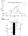
- FIG. 26 1 schematically shows a prior art TDR sensor 10 mounted as a level sensor in a tank or container 12 with a medium or liquid 14.
- the liquid 14 forms an interface 18 with respect to the air 16.
- the sensor 10 is designed to determine the distance of the interface 18 and to derive from its known mounting position the level and if necessary based on the geometry of the container 12 and the amount of liquid 14 ,
- the formation of the sensor 10 as a level sensor is a very important field of use, the sensor 10 can in principle also be used in other areas in which an interface is to be located.
- other boundary surfaces 18 are to be considered, for example bulk material or granules, or impurities in lines.
- the sensor 10 has a sensor head 20 with a controller 22, which is preferably accommodated on a common board. Alternatively, several circuit boards or flexprint carriers connected via plugs are conceivable.
- a coaxial probe 24 is connected, which has an outer conductor 26 and an inner conductor 28. In such a closed probe 24, the electromagnetic signals are guided particularly trouble-free.
- a different probe shape for example an open monosonde, which can be cleaned more easily.
- FIG. 27 shown in a block diagram.
- the actual control forms an FPGA 30, which may also be a microprocessor, ASIC or a similar digital logic module as well as a combination of several such components and in which the evaluation unit 32 is implemented.
- a pulse is transmitted to the inner conductor 28 via a microwave transmitter 34 and the transit time of the reflex pulse generated at the interface 18 and received in a microwave receiver 36 is measured to be the distance of the interface 18 and thus the fill level to determine the container 12.
- the received signal of the microwave receiver 36 is digitized for evaluation after amplification in an amplifier 38 with a digital / analog converter 40.
- the distance to more than one interface it is provided to determine the distance to more than one interface.
- the evaluation methods required for this purpose are implemented in the evaluation unit 32 and will be described below with reference to FIG FIGS. 1 to 25 explained in more detail.
- FIG. 1 shows an exemplary, recorded by a TDR sensor 10 waveform from a level measurement in a container with two stacked media.
- the waveform is called an echo curve in the image caption, because it is the system's response to a transmit pulse.
- an ideal curve without parasitic effects, EMC interference or other noise sources is drawn.
- an at least reasonably smooth curve can be achieved by analog or digital filtering.
- the extrema of the signal curve are used to measure the distance to the interfaces and the relative permittivity or the relative dielectric constant of the media.
- a first maximum is a pure artifact and will not be discussed further.
- the following maximum 42 arises at the beginning of the probe 24, which is also referred to below as the line input, and serves as an initial reference pulse.
- the transmission signal is reflected at the first interface to the first medium or at the second interface to the second medium in the container 12. From the end of the probe 24 comes a last maximum 48 as the final reference pulse.
- the later signal components are no longer relevant, further smaller extrema are higher orders of multiple reflections at the two interfaces. It is conceivable to use these extremes for plausibility, but mostly they are not suitable because of too low signal / noise ratio.
- Each extremum 42-48 is described by two parameters as shown, namely the amplitude A start , A refl Wed. , A end and the temporal position t start , t refl Wed. , t end .
- the superscript running index Mi stands for the ith medium.
- the initial reference pulse 42, the final reference pulse 48 and the reflection pulse 44 closest to the initial reference pulse 42 are searched from the first interface. From their amplitudes and temporal positions, the relative dielectric constant of the first medium is determined in two ways. to then compare the results and decide whether there is another medium in the container 12 under the first medium.
- a first method determines the relative dielectric constant ⁇ r ⁇ 1 M ⁇ 1 from the amplitudes A start of the initial reference pulse 42 and A refl M ⁇ 1 of the reflection pulse 44 at the first interface.
- the index ri stands for relative dielectric constant according to the ith method.
- Z L is the wave impedance of the air-filled space above the first medium
- Z l is the wave impedance of the first medium.
- a second method determines the relative dielectric constant ⁇ r ⁇ 2 M ⁇ 1 again independent of the difference between the time t refl M ⁇ 1 of the first reflection pulse 44 and the time t end of the final reference pulse 48.
- ⁇ r ⁇ 1 M ⁇ 1 and ⁇ r ⁇ 2 M ⁇ 1 match up to a previously defined tolerance limit ⁇ M 1 , that is, if: ⁇ r ⁇ 2 M ⁇ 1 - ⁇ r ⁇ 1 M ⁇ 1 ⁇ ⁇ M ⁇ 1 ,
- FIG. 2 illustrates such a situation with two superimposed media 14a-b, which also the exemplary waveform of the FIG. 1 equivalent. It shows some of the parameters used.
- the first medium 14a is foam forming a first interface 18a
- the second media 14b forming a second interface 18b is a liquid.
- the top layer is formed by air.
- Z 1 denotes the wave impedance in the first medium 14a
- Z 2 denotes the wave impedance in the second medium 14b.
- the dielectric constant determined by the first method becomes ⁇ r ⁇ 1 M ⁇ 1 used because the determined according to the second method relative dielectric constant ⁇ r ⁇ 2 M ⁇ 1 under the has now been calculated as a false hypothesis that there is only one medium in the container 12.
- the relative dielectric constant ⁇ r M ⁇ 2 is a still unknown size.
- FIG. 2 also illustrates the relationship between the amplitudes A start and A refl M ⁇ 2 ,
- a pulse having the amplitude A start At the first interface 18a, a pulse having the amplitude A start .
- the pulse component which proceeds further towards the end of the probe depends solely on the reflection coefficient r M 1 of the first interface 18a and amounts to A start ⁇ ( r M 1 + 1).
- This pulse portion strikes the second interface 18b, and a portion of the pulse is reflected back towards the first interface 18a.
- Its amplitude additionally depends on the reflection coefficient r M 2 of the second interface 18b and is A start ⁇ ( r M 1 + 1).
- r M 2 The returning wave hits the first interface 18a a second time from the opposite direction. In turn, a portion is reflected, while the remaining portion runs back towards the line input.
- r M ⁇ 2 A refl M ⁇ 2 A begin ⁇ r M ⁇ 1 + 1 2 ,
- the results become ⁇ r ⁇ 1 M ⁇ 2 and ⁇ r ⁇ 2 M ⁇ 2 Both methods compared with a tolerance threshold ⁇ M 2 .
- the measurement is with the results d begin M ⁇ 1 .
- d begin M ⁇ 2 for the distances to the two interfaces 18a-b and the relative dielectric constant ⁇ r M ⁇ 1 .
- ⁇ r M ⁇ 2 for the two media 14a-b, the latter corresponding, for example, to the result of one of the two methods or an average of both methods.
- a further medium below the second medium 14b is assumed.
- the procedure is repeated iteratively until all existing media have been found or until an abort condition is met.
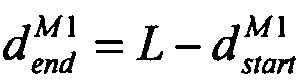
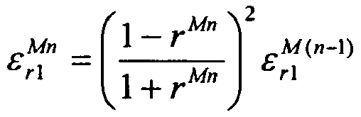
- the further iterations will only be briefly described in order to give generalized calculation instructions for the nth medium.
- d end Mn L - d begin Mn ,
- reflection pulses 44, 46 In order to estimate the parameters of reflection pulses 44, 46 as accurately as possible, it is provided in a development of the invention to operate the amplifier 38 with a non-linear characteristic. If the reflection pulses 44, 46 are then uniquely identified, the known effect of the non-linear amplification should be eliminated before quantitative evaluations of amplitude values.
- FIG. 4 represents the effect of amplification with a characteristic according to FIG. 3 on the waveform of the FIG. 1
- the two reflection pulses 44, 46 can obviously be separated better, because apart from the initial artifact no disturbing extrema occur more. However, already well-pronounced pulses like the initial artifact pulse are unnecessarily amplified disproportionately.
- the characteristic curve is therefore preferably to be adapted such that the amplitudes of the reflection pulses 44, 46 at the boundary surfaces are purposefully amplified and the remaining pulses are suppressed.
- a plurality of preferably continuously differentiable functions can be pieced together in order to specifically achieve the desired amplification of mean amplitudes in which measuring pulses 44, 46 lie and suppression of artifacts and noise.
- Pulse 42-48 are now very clearly identifiable.
- the final reference pulse 48 is somewhat less pronounced, but because of the known probe length it can be searched for in a quite narrow time range and thus nevertheless reliably detected. As long as the characteristic is monotonic, the position of the pulses 42-48 under non-linear amplification is maintained.
- Deviating and non-symmetrical non-linear characteristics can be defined according to the described guidelines.
- any piecewise function curves are conceivable, such as polynomial, exponential, logarithmic, hyperbolic or trigonometric functions.
- the discrete measured values are interpolated to obtain an analytical function and to increase the measuring accuracy of the sensor beyond the temporal resolution of the sampling times.
- a polynomial interpolation is not effective.
- FIG. 9 shows the waveform of the FIG. 1 mirrored and discretized on the Y axis and a sinc (x) interpolation for comparison.
- FIG. 10 is an enlarged detail, where the upper right of the entire waveform is shown in a pictogram with a rectangle 50, which indicates the position of the cutout. This form of representation is used in all subsequent detail enlargements to explain the interpolation. Of the FIG. 10 It can be seen that the sinc (x) interpolation generates relatively large interpolation errors despite its high cost.
- Another conceivable interpolation method consists in the piecewise interpolation using splines, in particular cubic C 2 -splines, which are thus twice continuously differentiable including their connection points.
- splines in particular cubic C 2 -splines, which are thus twice continuously differentiable including their connection points.
- FIGS. 11 and 12 demonstrate spline interpolation for the waveform in accordance with FIG. 1 very well. This quality is, however, bought by high numerical effort.
- a piecewise quadratic interpolation is used.
- FIGS. 11 and 12 In addition to spline interpolation, the just-derived piecewise quadratic interpolation is shown as a reference. In a section with greater variability according to FIG. 11 So larger gradients between each two nodes, the two interpolations are not distinguishable from each other. In the flatter section of the FIG. 12 On the other hand, in the piecewise quadratic interpolation, slight overshoots occur at the interpolation points introducing a small interpolation error. Note the different scale of the FIGS. 11 and 12 in Y-direction, the signal in FIG. 12 looks visually steeper than it is.
- a quadratic polynomial is used if the difference of the associated amplitude values exceeds a certain value ⁇ .
- the difference between the amplitude values of at least one of the two value pairs and the amplitude value at an additional support point in the environment must be a minimum value ⁇ . If these conditions are not met, the piece s i ( x ) is approximated by a linear polynomial.
- FIGS. 13 and 14 show again the excerpts of the FIGS. 11 and 12 with the difference that instead of the piecewise quadratic interpolation now the piecewise quadratic / linear interpolation is used.
- FIG. 13 Therefore, no differences are to be expected, because in this section the slope condition for quadratic interpolation is not violated or only in very few places, so that practically only quadratic interpolation comes into play.
- FIG. 14 a clear improvement recognizable.
- the linear approximation in areas of small slope does not show the disturbing overshoots and thus leads to a significantly lower interpolation error with even comparatively lower computational effort.
- the interpolation error is even greater than with spline interpolation. In the flat areas, however, the interpolation error is more acceptable anyway, since no reflection pulses 44, 46 are to be expected here.
- the different scale of FIGS. 13 and 14 in the Y direction Again, the different scale of FIGS. 13 and 14 in the Y direction.
- interpolation points ( x i , y i ) are taken into account if the difference between the amplitude maximum and minimum in an environment [ x i - ⁇ , x i + ⁇ ] of the interpolation point exceeds a minimum amount ⁇ : Max ⁇ y i - ⁇ ... y i + ⁇ - min ⁇ y i - ⁇ ... y i + ⁇ ⁇ ⁇ ⁇
- s j x ⁇ a j ⁇ x - x j 2 + b j ⁇ x - x j + c j .
- FIG. 15 shows the discretized waveform with the adaptive interpolation just described.
- ⁇ ⁇ x was set.
- no more support points are available. It should be noted that such subareas without support points can reach a considerable proportion of the total number of support points with a larger probe length.
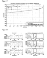
- FIG. 16 shows a part of the FIG. 15 in a region with large slopes, which interpolates with quadratic polynomials.
- the relevant quantities, namely amplitude and position of the maximum, can be clearly seen.
- FIG. 17 provides a comparison of the FIG. 15 in a low slope area. Due to the opposite FIG. 16 changed scale in the Y direction, the remaining slope of the waveform is still visually exaggerated. Almost all interpolation points are ignored and are bridged by a linear interpolation.
- the described adaptive interpolation avoids unnecessary effort in irrelevant subareas. interesting parts, on the other hand, are interpolated very precisely. The effort compared to spline interpolation or even sinc interpolation is considerably reduced. All described interpolation methods are equally applicable to linearly as well as non-linearly pre-amplified signal waveforms.
- the measurement of the distance to several interfaces requires that the individual reflection pulses 44, 46 are resolved exactly and their amplitude and position are determined as accurately as possible. This is particularly difficult when a medium forms a particularly thin layer, so that the reflection pulses of two interfaces overlap one another. A simple search for extremes not only runs the risk of overlooking an interface. Because of the deviant waveform of superimposed reflection pulses, the position of the maximum and thus its amplitude may also be incorrectly evaluated.
- FIG. 18 shows three conceivable special cases in which two reflection pulses are superimposed.
- the waveforms are linear or not amplified, in the right part of the FIG. 18 on the other hand reinforced with a non-linear characteristic.
- the earlier reflection pulse is less pronounced and leads only to an upstream shoulder of the later reflection pulse.
- a second special case is the temporal reflection to this, where the later reflection pulse is less pronounced and leads to a downstream shoulder.
- the two reflection pulses are completely fused into a single maximum.
- FIG. 19 shows the three special cases of the left part of the FIG. 18 , ie the linearly amplified signal waveforms, after this interpolation.
- the left part of the FIG. 19 represents the complete waveforms and the right part of the FIG. 19 the cutouts 50 is enlarged.
- FIG. 20 is analogous to the FIG. 19 Here are the three special cases of the right part of the FIG. 18 are based, so the non-linearly amplified signal waveforms. Again, the left part of the FIG. 20 the complete waveforms and the right part of the FIG. 20 the cutouts 50 are enlarged. In the non-linear amplification, the local maxima to be found are more distinguishable.
- a minimum duration is searched for after the first rising edge and its last point as in FIG. 21 shown as the first reference maximum 54 set.
- the reference maximum begins as in FIG. 22 shown a time window that ends after a predetermined duration at a time 56.
- the time window is chosen to be so large that two reflection pulses merged into one another, but a separated next reflection pulse is no longer detected.
- the window width can be fixed in advance independently of the specific measurement because of the known individual pulse shape and an expected maximum amplitude.
- the time window is searched for a falling edge 58 over a minimum period.
- the exact position of the local maximum is then determined. Since the waveform is described by the interpolation function, the position can be determined analytically with high accuracy.
- FIG. 24 shows the thus separated reflection pulses, where in the left part of detail enlargements and in the right part of the complete signal waveforms in the three special cases are shown.
- the amplitudes belonging to the positions determined in this way can be read out directly from the interpolation function.
- the amplitudes can still be falsified by the superimposition.
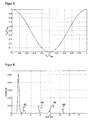
- FIG. 25 An optimization method is explained with which the superposition of reflection pulses is separated into the individual reflection pulses. Shown is, on the one hand, the superimposed signal profile 60 and, on the other hand, the two individual reflection pulses 62, 64 which form the superimposition. In the example of FIG. 25 Accordingly, the number n of the superimposed reflection pulses is two. It can clearly be seen that the amplitudes, in particular the amplitude of the second reflection pulse 64, would be overestimated only on the basis of the superimposed signal profile 60 without the separation shown.
- the shape of the transmission pulse S (t) and thus a single reflection pulse is known or is measured in advance.
- the invention preferably seeks to search not quite generally for the entire probe length for a large number of media but, for example, only for a small time window for two media, as in the case of the figure 25.
- FIGS. 18 to 24 described very good initial values of the free parameters known. This or part of these measures cause an optimization algorithm to converge rapidly in the global maximum.
- both the distances to the interfaces and the relative dielectric constants of the respective media forming the interfaces are known.
- the number of media is basically unlimited.
- Simple level meters usually have only switching output signals. In the configuration of the simple interface, it could be determined depending on which medium level in boundary layer measurements or depending on the medium or foam level in applications with foam formation, the outputs are controlled. Thus, useful functions for the application of the sensor can be realized:
- a container in which a liquid forms foam still contains a foam layer when emptying.
- Simple level sensors interpret this foam layer as residual liquid. Since the sensor 10 according to the invention knows the relative dielectric constant, a distinction is made between a residual layer of the liquid and a pure foam layer. Thus, a dry running protection of pumps can be realized, and conventionally specially provided for this function additional sensors in the pump lines are dispensable.
- a similar case occurs at high levels with foam or multiple media. Overflow of a container can occur when a simple level sensor overlooks a foam surface and only recognizes the underlying liquid surface with its comparatively high reflectivity. In contrast, the sensor according to the invention also dissolves the foam layer even including its layer thickness and can generate a switching signal as an overfill warning.
- the implementation of an overfill protection is desired for some applications, an approval according to WHG (Water Resources Act) even requires overfill protection.
- the determined relative dielectric constants can be used for quality control of the process in the container.
- the relative dielectric constants are made available to the application, for example via an interface, or the sensor offers corresponding setting possibilities for a signal at a switching output if certain criteria for the relative dielectric constants are violated or complied with.
- the sensor according to the invention recognizes but at the constant relative dielectric constant that within the same medium, another non-plausible reflection pulse is formed at the deposit.
- the sensor can already generate a warning or fault message at this time, in order to avoid the error situation later, when the level drops below the deposit. Such self-monitoring protects the system against further damage and increases its availability.
Landscapes
- Physics & Mathematics (AREA)
- Engineering & Computer Science (AREA)
- Radar, Positioning & Navigation (AREA)
- Remote Sensing (AREA)
- General Physics & Mathematics (AREA)
- Electromagnetism (AREA)
- Computer Networks & Wireless Communication (AREA)
- Thermal Sciences (AREA)
- Fluid Mechanics (AREA)
- Measurement Of Resistance Or Impedance (AREA)
Claims (15)
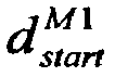
- Procédé pour la mesure de la distance par rapport à au moins une première surface limite (18a) par émission d'un signal électromagnétique le long d'une sonde (24), enregistrement de l'évolution du signal réfléchi et détermination de la distance (


caractérisé en ce que
la constante diélectrique relative (

- Procédé selon la revendication 1,
dans lequel la constante diélectrique relative est déterminée lors de la première fois en utilisant un coefficient de réflexion
la règle de calcul

- Procédé selon la revendication 1 ou 2,
dans lequel la distance (


- Procédé selon l'une des revendications précédentes,
dans lequel la distance (




- Procédé selon l'une des revendications précédentes,
dans lequel on ne cherche aucune autre surface limite quand l'un au moins des critères d'abandon suivant est rempli :- on a trouvé un nombre maximum de surfaces limite (18a-b),- la plus grande amplitude reconnue qui n'est pas encore attribuée à une surface limite (18a-b) dans l'évolution du signal passe au-dessous d'un seuil d'amplitude,- l'évolution du signal à l'intérieur d'une plage temporelle prédéterminée est entièrement évaluée,- l'énergie, intégrée depuis le commencement de la sonde (24) jusqu'à la surface limite évaluée en dernier lieu, de l'évolution du signal passe au-dessus d'un seuil d'énergie. - Procédé selon l'une des revendications précédentes,
dans lequel l'évolution du signal réfléchi est enregistrée de manière amplifiée avec une courbe caractéristique non linéaire, dans laquelle les signaux d'entrée d'amplitude moyenne sont amplifiés de manière surproportionnelle, les amplitudes moyennes étant définies par le fait qu'elles sont situées dans un intervalle au-dessus d'un niveau de bruit et au-dessous d'un signal de départ (42) ou d'un artefact (48) de l'extrémité de la sonde (24) comme étant le signal attendu le plus fort. - Procédé selon l'une des revendications précédentes,
dans lequel l'évolution du signal réfléchi est enregistrée de manière amplifiée avec une courbe caractéristique non linéaire, dans laquelle les signaux d'entrée de petite amplitude et/ou de grande amplitude sont supprimés, les petites amplitudes étant définies comme étant au-dessous ou au voisinage d'un niveau de bruit, et les grandes amplitudes étant définies comme ayant l'ordre de grandeur d'un signal de départ (42) ou d'un artefact (48) de l'extrémité de la sonde (24). - Procédé selon la revendication 6 ou 7,
dans lequel la courbe caractéristique pour des signaux d'entrée minimum et maximum est aplatie sur une portion d'amplitude maximum, est à zéro pour des signaux d'entrée voisins de zéro, et présente entre ceux-ci une évolution sigmoïde, ladite évolution sigmoïde étant en particulier imposée par un polynôme, les emplacements de jonction du polynôme vers les régions aplaties étant susceptible d'être dérivées, au moins en continu. - Procédé selon l'une des revendications précédentes,
dans lequel l'évolution du signal est numérisée tout d'abord avec des emplacements de soutien discrets, et est ensuite interpolée morceau par morceau par une famille de polynômes de second ordre entre deux emplacements de soutien respectifs, lesdits emplacements de jonction entre deux polynômes étant susceptibles d'être dérivés en continu. - Procédé selon l'une des revendications précédentes,
dans lequel, entre deux emplacements de soutien respectifs dans lesquelles la pente de l'évolution du signal est inférieure à une première pente minimum, on utilise pour l'interpolation un polynôme de premier ordre à la place d'un polynôme de second ordre. - Procédé selon l'une des revendications précédentes,
dans lequel, si dans les environs d'un emplacement de soutien la pente de l'évolution du signal est inférieure à une seconde pente minimum, l'emplacement de soutien reste sans être pris en compte dans la suite de l'interpolation. - Procédé selon l'une des revendications précédentes,
dans lequel les temps de parcours du signal (
- Procédé selon l'une des revendications précédentes,
dans lequel la situation exacte des maxima est déterminée de manière analytique à partir d'une interpolation de l'évolution du signal. - Procédé selon l'une des revendications précédentes,
dans lequel on forme une évolution de consigne du signal à partir d'une convolution du signal émis avec des impulsions delta pondérées par les amplitudes (


- Capteur (10), en particulier capteur de niveau TDR, comprenant un émetteur (34) et un récepteur (36) pour émettre et recevoir un signal électromagnétique, en particulier un signal à micro-ondes, et comprenant une commande (32) qui est réalisée pour déterminer la distance (


Priority Applications (1)
| Application Number | Priority Date | Filing Date | Title |
|---|---|---|---|
| EP20100154636 EP2365302B1 (fr) | 2010-02-25 | 2010-02-25 | Mesure de la distance par rapport à, au moins, une première surface limite |
Applications Claiming Priority (1)
| Application Number | Priority Date | Filing Date | Title |
|---|---|---|---|
| EP20100154636 EP2365302B1 (fr) | 2010-02-25 | 2010-02-25 | Mesure de la distance par rapport à, au moins, une première surface limite |
Publications (2)
| Publication Number | Publication Date |
|---|---|
| EP2365302A1 EP2365302A1 (fr) | 2011-09-14 |
| EP2365302B1 true EP2365302B1 (fr) | 2012-05-23 |
Family
ID=42320089
Family Applications (1)
| Application Number | Title | Priority Date | Filing Date |
|---|---|---|---|
| EP20100154636 Active EP2365302B1 (fr) | 2010-02-25 | 2010-02-25 | Mesure de la distance par rapport à, au moins, une première surface limite |
Country Status (1)
| Country | Link |
|---|---|
| EP (1) | EP2365302B1 (fr) |
Families Citing this family (11)
| Publication number | Priority date | Publication date | Assignee | Title |
|---|---|---|---|---|
| US8746045B2 (en) * | 2006-11-17 | 2014-06-10 | Meggitt (Orange County), Inc. | System and method for identifying fluids and monitoring fluid quality in a vessel |
| DE102012101725A1 (de) | 2012-03-01 | 2013-09-05 | Sick Ag | Verfahren zur Füllstandsmessung |
| US8963769B2 (en) * | 2012-10-16 | 2015-02-24 | Magnetrol International, Incorporated | Guided wave radar interface measurement medium identification |
| DK2759813T3 (da) | 2013-01-25 | 2016-06-06 | Sick Ag | Method and sensor for measuring the fill level of layered media |
| DE102013107847A1 (de) | 2013-07-23 | 2015-01-29 | Endress + Hauser Gmbh + Co. Kg | Verfahren zur Ermittlung und Überwachung des Füllstands eines Mediums in einem Behälter nach einem Laufzeitmessverfahren |
| DE102014103212A1 (de) * | 2014-03-11 | 2015-09-17 | Sick Ag | Sensor und Verfahren zum Erkennen eines auf einer Rollenbahn befindlichen Objekts |
| DE102015118917A1 (de) * | 2015-11-04 | 2017-05-04 | Finetek Co., Ltd. | Materialpegel-Messverfahren mit einer Materialpegel-Messvorrichtung |
| EA037645B9 (ru) * | 2016-08-22 | 2021-09-20 | Басф Се | Способ и устройство для обнаружения отложений в трубопроводной системе устройства |
| US10386180B2 (en) | 2016-11-28 | 2019-08-20 | Honeywell International Inc. | Apparatus and method for measuring thin material thicknesses in inventory management applications |
| DE102017108702A1 (de) * | 2017-04-24 | 2018-10-25 | Krohne S. A. S. | Verfahren zur Bestimmung des Füllstandes und Füllstandmessgerät |
| US10816384B2 (en) * | 2017-10-31 | 2020-10-27 | Rosemount Tank Radar Ab | Radar level gauge system and method for interface measurement |
Family Cites Families (3)
| Publication number | Priority date | Publication date | Assignee | Title |
|---|---|---|---|---|
| GB2153616B (en) * | 1984-02-01 | 1987-03-11 | Standard Telephones Cables Ltd | Liquid level measurement |
| US5884231A (en) * | 1995-12-21 | 1999-03-16 | Endress & Hauser Gmbh & Co. | Processor apparatus and method for a process measurement signal |
| US6198424B1 (en) * | 1999-01-21 | 2001-03-06 | Rosemount Inc. | Multiple process product interface detection for a low power radar level transmitter |
-
2010
- 2010-02-25 EP EP20100154636 patent/EP2365302B1/fr active Active
Also Published As
| Publication number | Publication date |
|---|---|
| EP2365302A1 (fr) | 2011-09-14 |
Similar Documents
| Publication | Publication Date | Title |
|---|---|---|
| EP2365302B1 (fr) | Mesure de la distance par rapport à, au moins, une première surface limite | |
| EP2634541B1 (fr) | Procédé de mesure de niveau de remplissage | |
| EP2759813B1 (fr) | Procédé et capteur de mesure du niveau de remplissage de supports stratifiés | |
| EP2652462B1 (fr) | Dispositif de mesure, dispositif de commande et appareil de mesure pour la mesure d'un niveau | |
| EP2527801B1 (fr) | Dispositif et procédé de détermination de caractéristiques de milieux et de récipients | |
| EP2527802B1 (fr) | Dispositif et procédé de détermination de caractéristiques de milieux et de récipients | |
| EP2366983B1 (fr) | Reconnaissance de mobilité dans un appareil de mesure de niveau | |
| WO2015018586A1 (fr) | Correction de la dispersion de radar fmcw dans un tube | |
| EP2626676B1 (fr) | Dispositif et procédé de correction d'un décalage | |
| WO2003016835A1 (fr) | Procede pour evaluer les signaux de mesure d'un appareil de mesure fonctionnant selon le principe du temps de propagation | |
| EP2104839A1 (fr) | Procédé pour déterminer et surveiller le niveau d'un fluide dans un récipient selon un procédé de mesure du temps de propagation | |
| EP2554956B1 (fr) | Suivi en fonction de la mobilité | |
| EP2652465B1 (fr) | Détermination de propriétés de fluide lors de la mesure d'un niveau de remplissage | |
| EP3025128B1 (fr) | Procédé pour déterminer et surveiller le niveau d'un fluide dans un récipient selon un procédé de mesure du temps de propagation | |
| EP2527805A1 (fr) | Dispositif d'évaluation et procédé de détermination d'une grandeur caractéristique pour la position d'une surface limite dans un récipient | |
| EP2372319A1 (fr) | Accumulation d'écho parasite dans des bruits de récipients | |
| DE102010042525A1 (de) | Verfahren zur Ermittlung und Überwachung des Füllstands eines Mediums in einem Behälter mittels eines Füllstandsmessgeräts nach einem Laufzeitmessverfahren | |
| EP2527804A1 (fr) | Procédé de reconnaissance d'échos multiples et d'échos de sol | |
| EP2327966A1 (fr) | Mesure de l'éloignement d'une surface limite | |
| EP2584324B1 (fr) | Appareil de mesure du niveau de remplissage et procédé de détermination d'un rapport fonctionnel entre différentes pistes | |
| EP2739946B1 (fr) | Relation lineaire entre pistes | |
| EP2182380B1 (fr) | Procédé de détection de la superposition de pointe dans un spectre discret d'un signal de repérage | |
| DE10211334A1 (de) | Verfahren zum Messen der effektiven Direktivität und/oder effektiven Quelltor-Anpassung eines systemkalibrierten vektoriellen Netzwerkanalysators | |
| DE102017123529A1 (de) | Verfahren zur Ermittlung des Füllstandes eines in einem Behälter befindlichen Füllgutes | |
| WO2014166747A1 (fr) | Détermination d'une courbe d'écho par une résolution différente selon les zones |
Legal Events
| Date | Code | Title | Description |
|---|---|---|---|
| PUAI | Public reference made under article 153(3) epc to a published international application that has entered the european phase |
Free format text: ORIGINAL CODE: 0009012 |
|
| AK | Designated contracting states |
Kind code of ref document: A1 Designated state(s): AT BE BG CH CY CZ DE DK EE ES FI FR GB GR HR HU IE IS IT LI LT LU LV MC MK MT NL NO PL PT RO SE SI SK SM TR |
|
| AX | Request for extension of the european patent |
Extension state: AL BA RS |
|
| 17P | Request for examination filed |
Effective date: 20111012 |
|
| GRAP | Despatch of communication of intention to grant a patent |
Free format text: ORIGINAL CODE: EPIDOSNIGR1 |
|
| GRAS | Grant fee paid |
Free format text: ORIGINAL CODE: EPIDOSNIGR3 |
|
| GRAA | (expected) grant |
Free format text: ORIGINAL CODE: 0009210 |
|
| AK | Designated contracting states |
Kind code of ref document: B1 Designated state(s): AT BE BG CH CY CZ DE DK EE ES FI FR GB GR HR HU IE IS IT LI LT LU LV MC MK MT NL NO PL PT RO SE SI SK SM TR |
|
| REG | Reference to a national code |
Ref country code: GB Ref legal event code: FG4D Free format text: NOT ENGLISH |
|
| REG | Reference to a national code |
Ref country code: CH Ref legal event code: EP |
|
| REG | Reference to a national code |
Ref country code: AT Ref legal event code: REF Ref document number: 559284 Country of ref document: AT Kind code of ref document: T Effective date: 20120615 |
|
| REG | Reference to a national code |
Ref country code: IE Ref legal event code: FG4D Free format text: LANGUAGE OF EP DOCUMENT: GERMAN |
|
| REG | Reference to a national code |
Ref country code: SE Ref legal event code: TRGR |
|
| REG | Reference to a national code |
Ref country code: DE Ref legal event code: R096 Ref document number: 502010000779 Country of ref document: DE Effective date: 20120719 |
|
| REG | Reference to a national code |
Ref country code: NL Ref legal event code: VDEP Effective date: 20120523 |
|
| REG | Reference to a national code |
Ref country code: LT Ref legal event code: MG4D Effective date: 20120523 |
|
| PG25 | Lapsed in a contracting state [announced via postgrant information from national office to epo] |
Ref country code: IS Free format text: LAPSE BECAUSE OF FAILURE TO SUBMIT A TRANSLATION OF THE DESCRIPTION OR TO PAY THE FEE WITHIN THE PRESCRIBED TIME-LIMIT Effective date: 20120923 Ref country code: CY Free format text: LAPSE BECAUSE OF FAILURE TO SUBMIT A TRANSLATION OF THE DESCRIPTION OR TO PAY THE FEE WITHIN THE PRESCRIBED TIME-LIMIT Effective date: 20120523 Ref country code: NO Free format text: LAPSE BECAUSE OF FAILURE TO SUBMIT A TRANSLATION OF THE DESCRIPTION OR TO PAY THE FEE WITHIN THE PRESCRIBED TIME-LIMIT Effective date: 20120823 Ref country code: FI Free format text: LAPSE BECAUSE OF FAILURE TO SUBMIT A TRANSLATION OF THE DESCRIPTION OR TO PAY THE FEE WITHIN THE PRESCRIBED TIME-LIMIT Effective date: 20120523 Ref country code: LT Free format text: LAPSE BECAUSE OF FAILURE TO SUBMIT A TRANSLATION OF THE DESCRIPTION OR TO PAY THE FEE WITHIN THE PRESCRIBED TIME-LIMIT Effective date: 20120523 |
|
| PG25 | Lapsed in a contracting state [announced via postgrant information from national office to epo] |
Ref country code: SI Free format text: LAPSE BECAUSE OF FAILURE TO SUBMIT A TRANSLATION OF THE DESCRIPTION OR TO PAY THE FEE WITHIN THE PRESCRIBED TIME-LIMIT Effective date: 20120523 Ref country code: PT Free format text: LAPSE BECAUSE OF FAILURE TO SUBMIT A TRANSLATION OF THE DESCRIPTION OR TO PAY THE FEE WITHIN THE PRESCRIBED TIME-LIMIT Effective date: 20120924 Ref country code: LV Free format text: LAPSE BECAUSE OF FAILURE TO SUBMIT A TRANSLATION OF THE DESCRIPTION OR TO PAY THE FEE WITHIN THE PRESCRIBED TIME-LIMIT Effective date: 20120523 Ref country code: GR Free format text: LAPSE BECAUSE OF FAILURE TO SUBMIT A TRANSLATION OF THE DESCRIPTION OR TO PAY THE FEE WITHIN THE PRESCRIBED TIME-LIMIT Effective date: 20120824 Ref country code: HR Free format text: LAPSE BECAUSE OF FAILURE TO SUBMIT A TRANSLATION OF THE DESCRIPTION OR TO PAY THE FEE WITHIN THE PRESCRIBED TIME-LIMIT Effective date: 20120523 |
|
| PG25 | Lapsed in a contracting state [announced via postgrant information from national office to epo] |
Ref country code: SK Free format text: LAPSE BECAUSE OF FAILURE TO SUBMIT A TRANSLATION OF THE DESCRIPTION OR TO PAY THE FEE WITHIN THE PRESCRIBED TIME-LIMIT Effective date: 20120523 Ref country code: NL Free format text: LAPSE BECAUSE OF FAILURE TO SUBMIT A TRANSLATION OF THE DESCRIPTION OR TO PAY THE FEE WITHIN THE PRESCRIBED TIME-LIMIT Effective date: 20120523 Ref country code: DK Free format text: LAPSE BECAUSE OF FAILURE TO SUBMIT A TRANSLATION OF THE DESCRIPTION OR TO PAY THE FEE WITHIN THE PRESCRIBED TIME-LIMIT Effective date: 20120523 Ref country code: EE Free format text: LAPSE BECAUSE OF FAILURE TO SUBMIT A TRANSLATION OF THE DESCRIPTION OR TO PAY THE FEE WITHIN THE PRESCRIBED TIME-LIMIT Effective date: 20120523 Ref country code: CZ Free format text: LAPSE BECAUSE OF FAILURE TO SUBMIT A TRANSLATION OF THE DESCRIPTION OR TO PAY THE FEE WITHIN THE PRESCRIBED TIME-LIMIT Effective date: 20120523 Ref country code: RO Free format text: LAPSE BECAUSE OF FAILURE TO SUBMIT A TRANSLATION OF THE DESCRIPTION OR TO PAY THE FEE WITHIN THE PRESCRIBED TIME-LIMIT Effective date: 20120523 |
|
| PG25 | Lapsed in a contracting state [announced via postgrant information from national office to epo] |
Ref country code: PL Free format text: LAPSE BECAUSE OF FAILURE TO SUBMIT A TRANSLATION OF THE DESCRIPTION OR TO PAY THE FEE WITHIN THE PRESCRIBED TIME-LIMIT Effective date: 20120523 |
|
| PLBE | No opposition filed within time limit |
Free format text: ORIGINAL CODE: 0009261 |
|
| STAA | Information on the status of an ep patent application or granted ep patent |
Free format text: STATUS: NO OPPOSITION FILED WITHIN TIME LIMIT |
|
| 26N | No opposition filed |
Effective date: 20130226 |
|
| REG | Reference to a national code |
Ref country code: DE Ref legal event code: R097 Ref document number: 502010000779 Country of ref document: DE Effective date: 20130226 |
|
| PG25 | Lapsed in a contracting state [announced via postgrant information from national office to epo] |
Ref country code: BG Free format text: LAPSE BECAUSE OF FAILURE TO SUBMIT A TRANSLATION OF THE DESCRIPTION OR TO PAY THE FEE WITHIN THE PRESCRIBED TIME-LIMIT Effective date: 20120823 |
|
| BERE | Be: lapsed |
Owner name: SICK A.G. Effective date: 20130228 |
|
| PG25 | Lapsed in a contracting state [announced via postgrant information from national office to epo] |
Ref country code: MC Free format text: LAPSE BECAUSE OF NON-PAYMENT OF DUE FEES Effective date: 20130228 |
|
| PG25 | Lapsed in a contracting state [announced via postgrant information from national office to epo] |
Ref country code: ES Free format text: LAPSE BECAUSE OF FAILURE TO SUBMIT A TRANSLATION OF THE DESCRIPTION OR TO PAY THE FEE WITHIN THE PRESCRIBED TIME-LIMIT Effective date: 20120903 |
|
| REG | Reference to a national code |
Ref country code: IE Ref legal event code: MM4A |
|
| PG25 | Lapsed in a contracting state [announced via postgrant information from national office to epo] |
Ref country code: BE Free format text: LAPSE BECAUSE OF NON-PAYMENT OF DUE FEES Effective date: 20130228 Ref country code: IE Free format text: LAPSE BECAUSE OF NON-PAYMENT OF DUE FEES Effective date: 20130225 |
|
| PG25 | Lapsed in a contracting state [announced via postgrant information from national office to epo] |
Ref country code: MT Free format text: LAPSE BECAUSE OF FAILURE TO SUBMIT A TRANSLATION OF THE DESCRIPTION OR TO PAY THE FEE WITHIN THE PRESCRIBED TIME-LIMIT Effective date: 20120523 |
|
| PG25 | Lapsed in a contracting state [announced via postgrant information from national office to epo] |
Ref country code: SM Free format text: LAPSE BECAUSE OF FAILURE TO SUBMIT A TRANSLATION OF THE DESCRIPTION OR TO PAY THE FEE WITHIN THE PRESCRIBED TIME-LIMIT Effective date: 20120523 |
|
| PG25 | Lapsed in a contracting state [announced via postgrant information from national office to epo] |
Ref country code: TR Free format text: LAPSE BECAUSE OF FAILURE TO SUBMIT A TRANSLATION OF THE DESCRIPTION OR TO PAY THE FEE WITHIN THE PRESCRIBED TIME-LIMIT Effective date: 20120523 |
|
| PG25 | Lapsed in a contracting state [announced via postgrant information from national office to epo] |
Ref country code: LU Free format text: LAPSE BECAUSE OF NON-PAYMENT OF DUE FEES Effective date: 20130225 Ref country code: HU Free format text: LAPSE BECAUSE OF FAILURE TO SUBMIT A TRANSLATION OF THE DESCRIPTION OR TO PAY THE FEE WITHIN THE PRESCRIBED TIME-LIMIT; INVALID AB INITIO Effective date: 20100225 Ref country code: MK Free format text: LAPSE BECAUSE OF FAILURE TO SUBMIT A TRANSLATION OF THE DESCRIPTION OR TO PAY THE FEE WITHIN THE PRESCRIBED TIME-LIMIT Effective date: 20120523 |
|
| REG | Reference to a national code |
Ref country code: FR Ref legal event code: PLFP Year of fee payment: 7 |
|
| REG | Reference to a national code |
Ref country code: AT Ref legal event code: MM01 Ref document number: 559284 Country of ref document: AT Kind code of ref document: T Effective date: 20150225 |
|
| PG25 | Lapsed in a contracting state [announced via postgrant information from national office to epo] |
Ref country code: AT Free format text: LAPSE BECAUSE OF NON-PAYMENT OF DUE FEES Effective date: 20150225 |
|
| REG | Reference to a national code |
Ref country code: FR Ref legal event code: PLFP Year of fee payment: 8 |
|
| REG | Reference to a national code |
Ref country code: FR Ref legal event code: PLFP Year of fee payment: 9 |
|
| PGFP | Annual fee paid to national office [announced via postgrant information from national office to epo] |
Ref country code: SE Payment date: 20200224 Year of fee payment: 11 |
|
| PGFP | Annual fee paid to national office [announced via postgrant information from national office to epo] |
Ref country code: IT Payment date: 20210226 Year of fee payment: 12 Ref country code: FR Payment date: 20210218 Year of fee payment: 12 |
|
| REG | Reference to a national code |
Ref country code: SE Ref legal event code: EUG |
|
| PG25 | Lapsed in a contracting state [announced via postgrant information from national office to epo] |
Ref country code: SE Free format text: LAPSE BECAUSE OF NON-PAYMENT OF DUE FEES Effective date: 20210226 |
|
| PG25 | Lapsed in a contracting state [announced via postgrant information from national office to epo] |
Ref country code: FR Free format text: LAPSE BECAUSE OF NON-PAYMENT OF DUE FEES Effective date: 20220228 |
|
| PGFP | Annual fee paid to national office [announced via postgrant information from national office to epo] |
Ref country code: CH Payment date: 20230307 Year of fee payment: 14 |
|
| PG25 | Lapsed in a contracting state [announced via postgrant information from national office to epo] |
Ref country code: IT Free format text: LAPSE BECAUSE OF NON-PAYMENT OF DUE FEES Effective date: 20220225 |
|
| REG | Reference to a national code |
Ref country code: CH Ref legal event code: PL |
|
| PG25 | Lapsed in a contracting state [announced via postgrant information from national office to epo] |
Ref country code: CH Free format text: LAPSE BECAUSE OF NON-PAYMENT OF DUE FEES Effective date: 20240229 |
|
| PG25 | Lapsed in a contracting state [announced via postgrant information from national office to epo] |
Ref country code: CH Free format text: LAPSE BECAUSE OF NON-PAYMENT OF DUE FEES Effective date: 20240229 |
|
| PGFP | Annual fee paid to national office [announced via postgrant information from national office to epo] |
Ref country code: GB Payment date: 20260219 Year of fee payment: 17 |
|
| PGFP | Annual fee paid to national office [announced via postgrant information from national office to epo] |
Ref country code: DE Payment date: 20260217 Year of fee payment: 17 |