EP3528443A1 - Method for calculating an estimate of a modulated digital signal and its reliability - Google Patents
Method for calculating an estimate of a modulated digital signal and its reliability Download PDFInfo
- Publication number
- EP3528443A1 EP3528443A1 EP19156763.5A EP19156763A EP3528443A1 EP 3528443 A1 EP3528443 A1 EP 3528443A1 EP 19156763 A EP19156763 A EP 19156763A EP 3528443 A1 EP3528443 A1 EP 3528443A1
- Authority
- EP
- European Patent Office
- Prior art keywords
- signal
- receiver
- soft
- parameters
- reliability
- Prior art date
- Legal status (The legal status is an assumption and is not a legal conclusion. Google has not performed a legal analysis and makes no representation as to the accuracy of the status listed.)
- Granted
Links
Images


Classifications
-
- H—ELECTRICITY
- H04—ELECTRIC COMMUNICATION TECHNIQUE
- H04L—TRANSMISSION OF DIGITAL INFORMATION, e.g. TELEGRAPHIC COMMUNICATION
- H04L25/00—Baseband systems
- H04L25/02—Details ; arrangements for supplying electrical power along data transmission lines
- H04L25/03—Shaping networks in transmitter or receiver, e.g. adaptive shaping networks
- H04L25/03006—Arrangements for removing intersymbol interference
- H04L25/03171—Arrangements involving maximum a posteriori probability [MAP] detection
-
- H—ELECTRICITY
- H04—ELECTRIC COMMUNICATION TECHNIQUE
- H04L—TRANSMISSION OF DIGITAL INFORMATION, e.g. TELEGRAPHIC COMMUNICATION
- H04L25/00—Baseband systems
- H04L25/02—Details ; arrangements for supplying electrical power along data transmission lines
- H04L25/03—Shaping networks in transmitter or receiver, e.g. adaptive shaping networks
- H04L25/03006—Arrangements for removing intersymbol interference
- H04L25/03178—Arrangements involving sequence estimation techniques
- H04L25/03312—Arrangements specific to the provision of output signals
- H04L25/03318—Provision of soft decisions
-
- H—ELECTRICITY
- H04—ELECTRIC COMMUNICATION TECHNIQUE
- H04L—TRANSMISSION OF DIGITAL INFORMATION, e.g. TELEGRAPHIC COMMUNICATION
- H04L25/00—Baseband systems
- H04L25/02—Details ; arrangements for supplying electrical power along data transmission lines
- H04L25/06—DC level restoring means; Bias distortion correction ; Decision circuits providing symbol by symbol detection
- H04L25/067—DC level restoring means; Bias distortion correction ; Decision circuits providing symbol by symbol detection providing soft decisions, i.e. decisions together with an estimate of reliability
Definitions
- the invention relates to a method for improving the calculation of the estimation of the symbols of a modulated digital signal and their reliability, for any task that requires such an estimate.
- the symbol estimation presented here can be used to derive an estimate of the channel (or some of its parameters) between the transmitter and the receiver. It can be used to derive an estimate of the signal or receiver parameters such as, for example, the clock offset, or the time of signal reception. It can also be used to derive link quality metrics, such as mutual information between the transmitted and received symbols, the reliability of the sent signal estimate, the signal-to-noise ratio or the signal-to-noise plus interference ratio. .
- the invention also relates to a method for suppressing interference within a signal received on a receiver. It applies in particular to equalization with an adaptive receiver equalizer type feedback decision or DFE (Digital Feedback Equalizer) for equalization of symbols received.
- DFE Digital Feedback Equalizer
- the field of the invention is that of digital radio communication systems and, inter alia, transmitters and receivers for multichannel communications, that is to say comprising several antennas.
- the invention also relates to multi-user systems in which the communication resources are shared between several users who can simultaneously communicate by sharing frequency bands or slots or time slots.
- the invention relates to all multi-user communication systems in which high levels of interference are generated both between transmitters associated with different users but also between the symbols conveyed by a signal transmitted by a user of the device. makes disturbances inherent to the propagation channel.
- the invention precisely relates to the field of interference suppression in a multi-user context in the context of iterative receivers, which consists in the iteration of the interference suppression and decoding functions in the objective final to improve the bit error rate or the packet error rate on the decoded symbols.
- the invention finds inter alia its application in cellular communication systems such as the 3GPP LTE system.
- the invention also aims at a method of equalization in the frequency domain and which is flexible, adapted to a single-user context, or multi-user and with a receiver implementing a treatment is non-iterative or iterative.
- a transfer of information from a source to a destination involves propagation through a channel which may be, for example, a radio channel, a wired channel (such as a coaxial cable), etc.
- Some propagation means generate inter-symbol interference on the received signal.
- the received signal sampled at a given moment after compensation of propagation delays and processing, and having a correct synchronization, not only contains the symbol sent (possibly amplified and with a phase disturbance) plus noise, but a mixture or linear combination of symbols sent.
- ISI intersymbol interference
- Many equalization methods are described in the prior art.
- the goal is to achieve optimal performance given by the adapted filter terminal (which is a lower bound on the packet error rate) while being easy to use.
- the algorithms must therefore have computing complexity, memory occupancy and processing latency compatible, both to the applications that use the receivers in question and to the constraints of the hardware platforms on which they are implemented.
- the technical problem is therefore to find algorithms that find a good compromise performance / complexity of implementation with respect to the targeted applications.
- equalizers There are several equalizer classes: linear equalizers, decision feedback equalizers (DFEs), interference canceling equalizers (Interference Cancellation), and maximum posteriori (MAP) detectors. ), or detectors that estimate a Maximum Likelihood Sequence Estimation (MLSE). These equalizers can be declined in iterative form. Particular iterative receivers are so-called “turbo" receivers, where there is a repetitive exchange of extrinsic probabilistic information between processing blocks, for example between the equalization block and the decoding block.
- Expectancy propagation EP can also be seen as a message passing algorithm known as the "message passing”, in particular as a generalization of the belief propagation algorithm (Belief Propagation - BP - in English). English) to cases of non-categorical probability distributions but belonging to the exponential family.
- this concept allows for better message passing with minimum average square error (MMSE) estimators.
- MMSE minimum average square error
- the reference [6] uses this new soft return in the context of a multiple-input multiple-output (MIMO) receiver, which makes it possible to better approach the MAP performance.
- MIMO multiple-input multiple-output
- reference [17] studies a return signal based on the concept of PE from the soft demodulator, for block linear equalizers in the time domain.
- the solution described in [17] requires the inversion of matrices that potentially have a large size and therefore with considerable computational and memory complexity.
- As part of the turbo-equalization reference [15] is an extension of the reference [17], with its defects in terms of complexity.
- Reference [16] deals with frequency equalization with EP in the multi-user case where the mobile transmitters are equipped with a single transmitting antenna.
- the return EP is calculated on a colored Gaussian distribution, that is to say, leaving each estimated symbol to the demodulator to have a measure of reliability specific to it. This forces the frequency receiver to have a very complex structure, requiring the inversion of a full matrix to each block of data.
- a less complex alternative receiver is also derived, with a least squares hypothesis, but the equalizer then deviates unusable when the propagation channel has spectral zeros.
- Gaussian division refers to a division between two Gaussian probability density functions, with a “normalization” of the resulting function so that the latter function is still a Gaussian probability density function. To describe this operation in the Gaussian case, it is sufficient to calculate the mean and the variance of the resulting probability density from the means and variances of the two probability densities considered.
- the method further comprises a step of deinterleaving and interleaving the soft information on the transmitted signal, during the iterative exchange between a soft demodulator and a soft input / output binary decoder.
- the method may further include an iterative step of estimating channel parameters, using the soft estimate of the transmitted signal and its reliability from the soft demodulator together with the received signal.
- the computation of the parameters of the P equalizers in the frequency domain can use the knowledge of the statistics of the interference between segments, estimated from the reliability of the returns of the soft demodulator.
- Residual interference between segments is regenerated, for example, using the returns of the soft demodulator, and subtracted from each of the P segments y p , before the step of conversion in the frequency domain.
- the method is used to suppress interference within a signal received on an SC-FDMA or SS-SC-FDMA receiver comprising a framing step using respectively SC-FDMA or SS-SC-FDMA modulation and a step of executing the method according to the invention.
- the method can also be used to suppress interference within a signal received on an SC or SS-SC type receiver comprising a framing step respectively using an SC or SS-SC modulation and a step of executing the process according to the invention.
- the turbo equalization technique consists in the iteration between the function of equalization, of soft demodulation (here also called demapper or soft demapping) and decoding, generally with the aim of improving the bit error rate (Bit Error Rate - BER) or the Packet Error Rate (PER) while controlling the complexity of the receiver.
- soft demodulation here also called demapper or soft demapping
- decoding generally with the aim of improving the bit error rate (Bit Error Rate - BER) or the Packet Error Rate (PER) while controlling the complexity of the receiver.
- the first variant embodiment is given, by way of non-limiting example, in the case of a single-input single output system or SISO (Single Input Single Output) illustrated in FIG. figure 1 .
- the system consists of a transmitter 10 and a receiver 20 both equipped with a single antenna on transmission and reception.
- the generic mono-antennary transmitter 10 for the SISO application is represented in figure 2 .
- the transmitter 10 takes information bits, b, the bits are coded in an encoder 11 with an error correction coder which can be a convolutional code, a turbo-code, or a parity check code.
- error correction coder which can be a convolutional code, a turbo-code, or a parity check code.
- LDPC Low-Density Parity Check
- the coded bits are interleaved with an interleaver 12.
- the interleaved bits are then modulated by a modulator 13.
- the modulator 13 outputs symbols drawn from a constellation .
- the modulated symbols are transmitted to a framing block 14 which organizes the data in blocks in a frame and which can also insert pilot sequences which will be used, for example at the receiver, for the estimation of the channel.
- the pilot sequences are generated by a pilot sequence generator 15.
- the framing block 14 implements a method of partial periodization of the data blocks which allows, on reception, to implement an equalizer in the frequency domain.
- the raster signal is transmitted to an RF radio channel, 16, for transmission by an antenna A e .
- the framing block 14 may use orthogonal frequency division multiplexing modulation (Orthogonal Frequency Division Multiplexing - OFDM) with a total of N subcarriers including M subcarriers used with a cyclic prefix (Cyclic Prefix - CP) and possibly a cyclic suffix (Cyclic Suffix - CS).
- the framing block can also implement a multiple access OFDM modulation, called in the OFDMA literature.
- the framing block can also set up a Single Carrier-Frequency Division Multiple Access (SC-FDMA) frequency-division multiple access single-carrier modulation, with M the number of sub-carriers used for precoding with a single carrier. Discrete Fourier Transform (DFT).
- DFT Discrete Fourier Transform
- the CPs and CSs can be substituted by a constant sequence (for example zeros, or pilot sequences) or evolving from one frame to another (for example by a pseudo-random method known to the users), which makes it possible to to still obtain a signal with the good property of partial periodicity on the extended data blocks with one of these sequences. It is also possible to consider the use of single-carrier modulation with Spectrally Shaped Single Carrier (SS-SC) or mono-carrier modulation with multi-access spectral shaping Frequency Division Multiple Access (SS-SC-FDMA), where the signal could be filtered in time, or in frequency, by a filter of formatting, after the addition CP / CS.
- SS-SC Spectrally Shaped Single Carrier
- SS-SC-FDMA mono-carrier modulation with multi-access spectral shaping Frequency Division Multiple Access
- Non-circularity is expressed formally by the fact that if x ( n ) is a random symbol of the constellation emitted at time n, then the expectation of the squared symbol is different from zero E [ x 2 ( n )] ⁇ 0.
- the quantity E [ x 2 ( n )] is also called pseudo-covariance in the literature This property extends to sampled or continuous signals as well.
- the invention thus applies to transmitters using complex constellations such as quadrature amplitude modulation (QAM), phase shift keying (PSK), phase change modulation and amplitude (Amplitude Phase Shift Keying - APSK); real constellations, such as Binary Phase Shift Keying (BPSK), or Pulse Amplitude Modulation (PAM).
- QAM quadrature amplitude modulation
- PSK phase shift keying
- real constellations such as Binary Phase Shift Keying (BPSK), or Pulse Amplitude Modulation (PAM).
- BPSK Binary Phase Shift Keying
- PAM Pulse Amplitude Modulation
- the technique can also be applied to periodically rotated constellations like the ⁇ / 2-BPSK, where on the even symbols we use a classical BPSK constellation ⁇ +1, -1 ⁇ and on the odd symbols we use a rotated constellation of ⁇ / 2 radians ⁇ + j, - j ⁇
- constellations called quasi-rectilinear that is to say constellations whose symbols can be obtained by complex filtering of a signal described by the symbols of a real constellation .
- MSK Minimum Shift Keying
- GMSK Gaussian Minimum Shift Keying
- CPM Continuous Phase Modulation
- Offset Quadrature Amplitude Modulation - OQAM Offset Quadrature Amplitude Modulation - OQAM
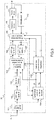
- the figure 3 illustrates a block diagram of the receiver 20 in the case where the transmitted signal is obtained with an SC-FDMA technique with prefix CP. It is assumed here that the signal of the transmitter is synchronized to the receiver with adequate accuracy (ie less than the duration of the CP, if present) and that a synchronization algorithm has provided the synchronization time to the receiver. The signal supplied as input to the block 101 is therefore already synchronized in time and frequency and at the right sampling frequency.
- the receiver can be used to receive a SS-SC-FDMA type signal.
- this receiver can be used in an SC system with CP.
- the receiver can be used to receive a SS-SC type signal.
- the "CP suppression" block is substituted by a "Processing block extraction” block which extracts the known sequences (for example to use them to estimate the channel) and the blocks of data to be processed, then the receiver can receive SC signals and SS-SC with known pilot sequences in place of CPs and CSs.
- the receiver is adapted to receive an OFDM or OFDMA type signal.
- the receiver according to the invention contains two feedback loops.
- the first loop is positioned between the DFE equalizer 108 and the SISO 105 soft demodulator.
- the course of this loop is called “self-iteration” and an equalizer that uses this loop is a “self-iterated equalizer”.
- the second loop is located between the soft demodulator SISO 105 and the decoding block decoder 111.
- the path of this loop is referred to as the "turbo-iteration” and an equalizer that uses this loop is a " turbo-iterated equalizer "or a" turbo-equalizer ".
- the invention realizes a self-iterated equalizer, of the DFE type, which is typically used with a priori null information at the level of the flexible demodulator.
- the numbers of auto-iterations or turbo-iterations set the trade-off between performance, computational complexity and required memory within the receiver.
- the equalizer filter ⁇ ( ⁇ , s ) indicates the filter used for turbo-iteration ⁇ and self-iteration s . This said, in the following, to simplify the notation, the apex will not be explicit, and we will implicitly refer to the current turbo-iteration and auto-iteration.
- the blocks must be initialized at the beginning of the reception processing and at the beginning of each turbo-iteration, so for each
- the data blocks After extracting the data blocks from the receiving antenna A r of the receiver, by deleting the CP in the case of SC systems with CP or SC-FDMA, 101, the data blocks pass through a Fast Fourier Transform (FFT) of size N (frequency domain transition).
- FFT Fast Fourier Transform
- the signal at the output of the FFT then goes into a block "De-alloc sub-p" 103 which makes it possible to access the M frequency resources (sub-carriers) among N, through which the signal has been transmitted.
- This block selects only the sub-carriers on which the signal has been transmitted (de-allocation of the sub-carriers), and at the output of this last dis-allocation block 103 the signal is represented by a vector y of size M, grouping the subcarriers used.
- the pilot sequences are extracted from the signals coming from the reception antenna A r and sent to the block "Estimation of the channels and the variance of the noise” 104. They are used to calculate an estimate of the frequency response of the channel between the transmitter and the receiver, on the M sub-carriers of interest (those used by the user to send the information).
- the block "Estimation of the channels and noise variance "104 also provides an estimate of the variance of noise. This noise contains the contribution of thermal noise on the receiving antenna A r and possible interference due to several spurious effects from either digital processing or other external signals.
- the block "Estimation of the channels and the variance of the noise” provides the covariance matrix of the noise in the frequency domain ⁇ w . Typically, there is a noise channel and covariance estimate per block of data.
- the deinterleaver block 110 is not calculated during the initialization phase.
- the estimate of the channel H and the estimate of the covariance matrix of the noise are then transmitted to the block "calculation of the parameters of the equalizer" 106.
- This block also takes as input the quantity v from the flexible demapping which measures the average reliability of the symbols sent by the user inside the data block which is being processed (the average is thus on the length of block M in the case of the example) .
- the "equalizer parameter calculation" block 106 outputs at each self-iteration the coefficients of the equalizer f of size M in the frequency domain, which is general a self-iterated linear MMSE turbo-equalizer with EP feedback.
- ⁇ m are the coefficients of the filter f .
- the received signal vector y of size M is passed into the block "linear interference suppression equalizer” 108 which also takes the coefficients of the filter of the equalizer ⁇ , the frequency response of the channel H and the size vector M soft estimates of symbols emitted in the frequency domain x , which is generated by the normalized FFT block of size M 107 from the vector of size M of flexible estimates in the time domain x , from the SISO 105 soft demodulator.
- the overall reliability of this estimate is represented by the value v the closer it is to zero, the greater the reliability ( v is a variance).
- the interference canceling linear equalizer block 108 performs Interference Cancellation (IC) for the ISI, in this case SISO.
- IC Interference Cancellation
- the interference canceling linear equalizer block 108 produces a vector of size M x which represents an estimate of the symbols in the frequency domain.
- the vector x is then passed back into the time domain through a standardized IFFT 109 of size M, to obtain the vector x of the equalized time signal, which is sent to the soft demodulator SISO 105.
- the soft demodulator From x , the variance of the noise after equalization ⁇ ⁇ 2 and a priori soft information, for example in the form of Log Likelihood Ratio (LLRs) L a metrics from the decoder, the soft demodulator produces soft information for each bit of the input signal, for example in the form of extrinsic LLR L e .
- LLRs Log Likelihood Ratio
- This demodulator takes different forms according to the statistics of the signal after equalization: if the starting constellation is real one can use a demodulator for symmetric complex Gaussian statistics, otherwise a demodulator for Gaussian statistics with non-zero pseudo-covariance is more suitable.
- the soft metrics are then deinterleaved by the de-interleaver block 110 which is the inverse block of the interleaver block 112. Then, when all the bits of the packet are retrieved, the soft metrics are sent to the decoder 111 which generates, produces bit probabilities estimates sent information (for example, posterior probabilities). These probability estimates can be used to obtain a hard estimate b ' of transmitted bits b with a threshold detector. If the receiver uses turbo-iterations, the decoder also produces estimates of the sent coded bits, ie extrinsic probabilities (EXT), for example in the form of LLRs, which measure the probability that the coded bits sent 0 or 1.
- EXT ie extrinsic probabilities
- the EXTs are then sent to the interleaver 112 to be interleaved.
- the interleaver 112 located in the receiver 20 operates in the same manner as the interleaver 12 in the transmitter 10, with the only difference that it operates on binary data, while the interleaver 112 operates on LLRs .
- the interlaced EXTs become information a priori from the point of view of the rest of the receiver, for example in the form of LLRs a priori L a and enter the flexible demodulator SISO 105.
- SISO 105 the flexible demodulator
- the interference canceling linear equalizer block 108 performs interference suppression and applies linear frequency equalization to the input signal.
- linear equalizer with interference suppression Linear Equalizer - Interference Cancellation - LE-IC
- This structure is already well known in the literature [2].
- the difference from the existing state of the art is in the value of the input x (estimation of symbols in the frequency domain) supplied to block 108, as well as the filter used, these two quantities being calculated in a new way.
- the output x of the interference canceling linear equalizer block 108 will therefore be different than that which can be found in [2] equal to the other hypotheses.
- the figure 4 provides a detailed example for the filtering and the interference removal method, which is efficiently performed as follows.
- the block "linear equalizer interference suppression" 108 comprises a subtractor 201 which acts on vectors of size M and which subtracts from the actually received signal y, an estimate of this same received signal (useful signal with interference of the propagation channel) .
- This allows to obtain a corrective signal input into a linear filter 202 MMSE type of frequency response ⁇ , calculated by the calculation block of the equalizer settings 106.
- the linear filter 202 is itself followed by a summer 203 vectors of size M, which reintroduces into the filtered corrective signal the contribution of the useful signal already estimated.
- the retrenchment block of the estimated received signal 201 obtains the estimate to be subtracted by a generation module of the estimated received signal (useful signal with interference of the propagation channel) 200.
- the summator 201 implements a retrenchment in the frequency domain of the received signal estimated at the received signal, y - h ⁇ x . The result is named corrective signal.
- Block 202 simply applies the filter f .
- This again is simply a multiplication entered by input of the vector of the filter size M and the input vector of the same size. This step corresponds to the equalization itself which further reduces the residual ISI of the corrective signal.
- the structure of the SISO 105 soft demodulator is illustrated in FIG. figure 5 .
- a constellation potentially multidimensional, here the invention is presented with a constellation with a complex dimension
- the modulator in the transmitter 10 from each vector of q bits coded and interleaved at the output of the interleaver block 12, generates the corresponding symbol of the constellation according to a function , which is also called function labeling or simply labeling, a concept known to those skilled in the art.
- d m [ d mq , ..., d ( m + 1 ) q- 1 ] is the m- th group of q elements of the vector d which is the vector of coded and interleaved bits of size qM corresponding to the block of data.
- the bit vector d m can be interpreted as the binary tag of the symbol x m .
- the figure 5 describes a detailed example for the structure of the soft demodulator.
- the at ⁇ d represents the vector of the LLRs a priori on the coded and interleaved bits, coming from the decoder and which are associated with the estimated signal vector after equalization x ( ⁇ , s ) being processed.
- L a ( d ) is a vector of zeros (no prior information on the available bits d ).
- the computation chain constituted by a calculation block of the a priori distributions 300, a block of soft estimates 301, an averaging estimator averaging 302 and a switch 303 is activated.
- This calculation chain is no longer activated for the other indices s ⁇ 0, but only when a new initialization is learned. During the initialization phase, in normal operation the other blocks are not activated.
- the calculation block of prior distributions 300 performs the computation of mass probabilities (probability distributions) a priori on the symbols of the constellation (this block is known from the state of the art) from L a ( d ) .
- mass probabilities probability distributions
- a priori on the symbols of the constellation (this block is known from the state of the art) from L a ( d ) .
- the soft estimate block 301 calculates an estimate of the transmitted symbols, as well as an estimation of their reliability, starting from the input probability distributions. Since all the distributions a priori P m ⁇ ⁇ (for all the symbols of all the data blocks composing the same code word) changes only with each turbo-iteration, block 301 is applied to P m ⁇ ⁇ only once per turbo-iteration and produces the following estimates: with the standard definitions of hope E P m ⁇ ⁇ and variance Var P m ⁇ ⁇ .
- switch 303 If s ⁇ 0, switch 303 outputs the symbol estimates x ⁇ m ⁇ , s + 1 and their average variance v ( ⁇ , s +1) from the adaptive smoothing block 307.
- s -1
- the output of the switch 303 therefore corresponds to the output of a flexible mapping with soft information from of the decoder, as described in reference [2].
- the exit The e ⁇ d is not calculated during the initialization phase. Once the outputs of the switch 303 are calculated, it is assumed that the input index s is incremented by 1.
- the processing chain consisting of blocks 304, 305, 301, 302, 306, 307 and 303.
- the likelihood calculation block 304 calculates likelihoods from the estimates x ⁇ m ⁇ s (the M equalized symbols of the current block) and the residual noise variance after equalization ⁇ v 2 ⁇ s , using an unbiased Gaussian model for estimates x ⁇ m ⁇ s . Note that it is described in the state of the art how to use a biased Gaussian model. This calculation gives: The m ⁇ s x ⁇ m ⁇ s
- the posterior probability distribution calculation block 305 comprises a first non-normalized posterior probability distribution calculation block 305A and a second block 305B whose function is to normalize the values supplied to its input in such a way that the output is a true probability distribution (see Fig. 5 ).
- the non-normalized posterior probability distribution block 305A calculates the distributions of the transmitted symbols by knowing observation (equalized symbols), according to a method known to those skilled in the art: where ⁇ is one of the possible symbols of the constellation .
- the block of soft estimates 301 calculates the estimates ⁇ m ⁇ s and the average variance ⁇ ( ⁇ , s ) symbols using as input a probability distribution obtained by normalizing (305B, equation (10)) the Gaussian likelihoods obtained by an exact or approximated calculation technique (304).
- the new estimation of the emitted symbols, generated by combining the a priori information available with the information contained in the observation according to the invention has characteristics superior to the estimate a priori. , or an estimate derived from the single observation.
- this operation also makes it possible to project a mixed probabilistic description on the sent symbols (Gaussian variables for the observations, combined with a priori estimates which are categorical variables) on a single probabilistic description, according to a Gaussian model as described in reference [3].
- Reverse I-projection or “M-projection” which states that finding an exponential-type distribution ( in our case, Gaussian) which minimizes the divergence of Kullback-Leibler (a measure of probabilistic distance) with respect to any distribution, amounts to finding the exponential distribution having the same statistical moments ("moment matching").
- the posterior mean variance allows both a more robust estimator of the average reliability of the estimated transmitted symbols of the data block and also the ability to implement a Frequency domain equalization strategy, generally less expensive from a computational point of view.
- Post hoc estimates ⁇ m ⁇ s Emitted symbols and their posterior average variances ⁇ ( ⁇ , s ) are then sent to the "Gaussian division" block 306 which also takes as input the observations (equalized symbols) x ⁇ m ⁇ s and the variance of residual noise after equalization ⁇ v 2 ⁇ s which gives a measure of the reliability of these observations.
- the Gaussian division using estimates as averages and reliabilities as variances, associates with each symbol two functions of Gaussian probability density, one for the posterior estimates and the other for the observations, divides them between it and the norms in order to obtain a third Gaussian probability distribution function having as a mean a new flexible estimate of the transmitted signal x ⁇ ' m ⁇ , s + 1 , and as variance the corresponding measure of reliability per block of data v ' ( ⁇ , s +1) .
- this block will generate an extrinsic information on the emitted symbols, following a Gaussian model.
- the solutions of the state of the art use either a priori information (categorical, extrinsic of the decoder), or a posteriori information (also categorical, combined extrinsic information of the decoder and the likelihood of the flexible demodulator).
- This operation therefore makes it possible to better respect the turbo principle by subtracting from the information a posteriori, the information a priori available to the demodulator, at the beginning of the processing (it is the extrinsic of the equalizer) and thus allowing improve the quality of the feedback signal and, ultimately, the performance of the receiver.
- the block 306 may output as a priori information from the decoder, calculated at the initialization of the flexible demodulator SISO (not shown in FIG. figure 5 ), as well as the average variance associated with the a priori as reliability. Still other strategies in the same case are to set the output variance v ' ( ⁇ , s +1) has an arbitrary value prefixed for each ⁇ and s .
- extrinsic estimates are passed to the adaptive smoothing block 307 whose purpose is to smooth the input estimates by taking past values into account.
- the z -1 blocks that are on the loop, in the figure 5 represent the operation of unit delay, vis-à-vis the index s , with reference to the transform Z.
- ⁇ a null function
- ⁇ (.) which remains constant, close to one, during the initial few iterations, then decreases linearly after deciding that the erroneous fixed points will not be fixed. taken into account.
- adaptive filters for example of the Kalman type.
- Yet another method is to dynamically read the parameters ⁇ ⁇ , s in a pre-filled table and stored in the memory of the equipment.
- pre-filled values of the parameters ⁇ ⁇ , s can be indexed according to one or more parameters of the receiver (for example the index of the current self-iteration or the current turbo-iteration) or of one or more metrics that the receiver can measure, such as the estimated channel, the noise estimate or the reliability of the returns of the decoder for example, and then use their values to dynamically choose the values of the corresponding ⁇ ⁇ , s .
- the adaptive smoothing block 307 generates extrinsic smoothed estimates.
- the SISO 105 soft demodulator After performing SISO 105 soft demodulation, the decoding process will be initiated. In this case, the SISO 105 soft demodulator outputs, for each new turbo-iteration with the decoder, extrinsic LLRs. The e ⁇ d on the coded bits of the processed data block. In this phase, the switch block 308 is closed and only the block 309 and the adder 310 are used. It is not necessary to calculate the other outputs of block 105.
- the The e ⁇ d are generated from the posterior LLRs calculated by block 309 and subtracting LLRs a priori The at ⁇ d through block sum 310.
- the block of calculation of posterior LLRs 309 is a known block of literature: Other logarithmic bases and methods of simplification of calculations are also applicable.
- the figures 6 and 7 illustrate an exemplary performance of the invention in a case of SC system with synchronization and perfect channel estimation, in the SISO framework.
- the constellation used by the transmitter is an 8-PSK
- the propagation channel is the Proakis C channel (with average power normalized to one) with a power profile of the type triangular (1, 2, 3, 2, 1).
- the figure 6 in particular shows the performance with without turbo-iteration, and with turbo-iterating once with decoder. In both cases the gains are considerable.
- FIG. 7 illustrates the performance with turbo iterations.
- the proposals considered come closer to the adapted filter terminal than the linear frequency MMSE turbo-equalizer with IC.
- the invention can be applied to a fractional turbo equalizer, for example see [8].
- the signal from the antenna is oversampled with a factor with a factor o > 1, typically an integer.
- the data blocks will therefore have a size oN in the FFT 102, oM in the inverse IFFT 109 and in the FFT 107.
- the IFFT block 109 is followed by a flow sampler o and the FFT block 107 is preceded by an ideal interpolator of factor o (which introduces o - 1 zero between two incoming samples).
- the "channel estimate and noise variance" block should make its estimates in the interpolated domain including possible transmit and receive filters, and then possibly pass the frequency estimates.
- the calculation of the parameters of the equalizer will carry out the calculations of the filter in the oversampled domain, on the other hand it will estimate the variance of the residual noise of equalization at the symbol time (to pass it to the flexible demodulator).
- the turbo block equalization 108 goes therefore work in the oversampled field.
- the SISO 105 soft demodulation block retains the foregoing description.
- the invention can be applied to an overlap equalizer FDE [9].
- FDE overlap equalizer
- the data block between two pilot sequences is longer than the processing block, and for complexity or necessity issues (for example a time-varying channel that changes in the horizon of a block of data), the frequency equalization process is broken down into several segments (with overlapping) of the initial data block. These segments suffer from interference between them. This implies that the noise covariance matrix at the output of the "channel estimate and noise variance" block 104 also includes the variance due to the interference, which modifies the values of the equalization filter.
- the channel estimate and noise variance block 104 can implement channel estimation and noise variance methods by exploiting this information additional.
- the new channel and noise variance estimates can be exploited by the rest of the receiver as described above.
- the proposed technique can also be applied to linear equalizers in the broad sense.
- the invention can be used within any type of iterative receiver being structured as illustrated in FIG. Figure 8 .
- This estimator extracts the signal y, the pilot sequences, in order to use one of the estimation techniques, known to those skilled in the art, to obtain parameters characterizing the channel.
- the estimate x is obtained through an interference suppression method which, using a prior estimate x the transmitted signal x , and an estimate of the channel parameters, generates an estimate of the interference and subtracts it from the received signal.
- a 503 receiver parameter calculation block is available, which uses the channel estimates and the reliability of the preliminary estimate. v , to calculate the intrinsic parameters of the receiver 502, and to calculate the variance ⁇ v 2 characterizing the residual interference power v at the output of the receiver 502.
- the invention applies at the level of the soft demodulator 504, where, for a data block with supposedly white statistics, the expectation propagation technique is used to calculate the flexible estimates x which will serve as feedback for the receiver, with the variance v characterizing the reliability of these same estimates.
- the soft demodulator 504 calculates extrinsic bit LLRs on the symbol-determining bits that can be used to estimate bits transmitted through a hard decision 505, comparing each binary LLR to zero.
- the soft input / output binary decoder block 507 is used in conjunction with the soft demodulator 504, and the adaptive receiver 502, in an appropriately selected scheduling, to assist in decoding the information bits of the transmitter.
- the two-loop scheduling described above for the SC-FDMA application could be used.
- the blocks of the interleaver 506 and interleaver 508 are included in the iteration loop between the soft demodulator 504 and the decoder 507.
- the estimates can be considered as x and reliability v at the output of the soft demodulator 504 are also directed to the channel estimator 501 (dashed arrows on the figure 8 ).
- the estimator 501 can use, from the first self-iteration of the receiver, the estimate x of the transmitted signal, together with the observation of the y- channel , to refine the parameters of the estimated channel, for example with a "least-squares" method on the entire data block, instead of using only the pilots.
- the invention relates, in particular, to the technique of estimating the transmitted signal, at the level of the flexible demodulator 504 which works on a model equivalent to a Gaussian additive noise.
- She may be used in any iterative receiver that goes through such a demodulation step and differs from hard demodulators, used inter alia in conventional decision feedback equalizers, which are subject to error propagation problems.
- the technique considered here is also different from the flexible demodulation techniques using a posteriori estimation of the signal, which do not remove from the estimation of the signal of return the information already known by the receiver, thus inducing the receiver to the error by biasing it with its own information.
- the method according to the invention provides an average reliability per block of data, which makes the receiver less complex and more robust to errors. one-off estimation.
- the invention applies adaptive smoothing on the estimated signal to provide an additional degree of freedom that allows the ratio of robustness of performance to convergence speed of the receiver to be compared to the limiting performance.
- the invention also applies to the single-user single-input multiple output (SIMO) case, that is to say to a communications system with a single transmitter and a single receiver using R antennas at reception.
- SIMO single-user single-input multiple output
- the invention also applies to the multiple input multiple-output (MIMO) multiple-user case where the single transmitter is provided with several, T u , transmission antennas.
- MIMO multiple input multiple-output
- T u 1
- R can be equal to one or more.
- U users transmit to the receiver and use the same time and frequency resources.
- the system is represented in figure 9 .
- This type of system is also called distributed Multiple Input Multiple Output (MIMO) system or virtual MIMO, or simply MIMO. If these users use separate time and frequency resources, allowing the receiver to see their signals without interference (ie orthogonal), the receiver can treat each of the users as an independent single-user SIMO / SISO system.
- MIMO distributed Multiple Input Multiple Output
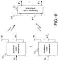
- the invention also applies to a multi-user wireless transmission system, where the users u (10 1 ,... 10 u ) are provided with one or more antennas (T u ⁇ 1) and the receiver 20 is provided with R antennas or R ⁇ 1.
- T u ⁇ 1 the users transmit to the receiver and use the same time and frequency resources.
- the system is represented in figure 10 .
- This type of system is also called Multi-User MIMO system (MU-MIMO). If these users use separate time and frequency resources, allowing the receiver to see their signals without interference (ie orthogonal), the receiver can treat each of the users as an independent single-user Multiple Input Single Output (MISO) system. In this case, only the interference between the antenna signals of the same transmitter will be present or non-negligible.
- MISO Multiple Input Single Output
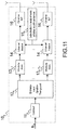
- the figure 11 illustrates the case of a generic multi-antenna transmitter 10 u , and the associated functional block diagram.
- the corrector error coder 11 u used in this case is not subject to constraints different from those of a single-antenna transmitter, it takes input bits of information, and provides encoded bits output.
- the spatio-temporal interleaver 12 provides u T u flow independent interleaved bits output.
- Each of the interleaved bit streams is then modulated by a modulator 13 u, 1 , 13 u, Tu dedicated to each antenna which outputs symbols drawn from a constellation , which can be different from one antenna to another and from one user to another.
- Remarks on the constellations to which the invention is still applicable extends to the case of each of T u modulators of a multi-antenna transmitter.
- the framing blocks 14 organize the symbols using the same strategy for each of the antennas.
- Block 15 u generator pilot sequences is extended to the multi-antenna case, with an ability to provide distinct pilot sequences for different antennas. Examples of given modulations, such as OFDM, (SS) -SC-FDMA or (SS) -SC, remain valid.
- each of the signals prepared for an antenna is passed through a radio frequency chain (RF) 16, identical for each antenna, and transmitted.
- RF radio frequency chain
- the correction code, the interleaver, the modulator and the generation of pilot sequences may have different characteristics chosen according to the user.
- the modulator may have different characteristics chosen according to the transmitting antenna for a given user.
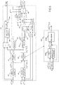
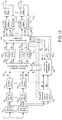
- the figure 12 represents a functional block diagram for the receiver in the case where the transmitted signal is obtained with an SC-FDMA technique with CP.
- this receiver can be used in an SC or SS system -SC or SS-SC-FDMA with CP.
- the receiver is adapted to the different types of SC systems with pilot or constant sequences instead of the CPs. . It is assumed here that the signal of the transmitter is synchronized to the receiver with adequate reliability (ie less than the duration of the CP, if present) and that a synchronization algorithm provided the synchronization instant to the receiver.
- the MU-MIMO receiver of the figure 12 contains two feedback loops: an auto-iteration loop (soft-mount / equalizer iteration) and a turbo-iteration loop (soft-mount / decoder iteration).
- the receiver in the presence of several users, the receiver must decide, for each loop, the users whose signals will be decoded / processed and which signals will not be decoded / processed.
- the groupings of users in the partition can be made according to several possible metrics, for example users scheduled according to the power of reception of their signals, or according to a metric derived from the power of reception of their signals and the reliability / variance of their constellations, or metrics based on differences in reception power and reliability between user pairs, etc.
- This block has all the T signals estimated as input.
- the receiver therefore tries to decode u i having the soft information of decoding already for all u j with j ⁇ i.
- a per-user encoder as in figure 11 .
- the same mechanism can be used to schedule the decoding of the antenna signals of all users together .
- Quantities exchanged by the iterative receiver of the figure 12 generally depend on the index of self-iteration, turbo-iteration and the scheduling of users to decode within a given turbo-iteration (especially users already decoded within the same turbo iteration) .
- the turbo-iteration index is incremented when all users have been decoded (the entire partition of all users has been browsed according to the established order function).
- the equalizer filter f t , u ⁇ i s indicates the filter to be applied to equalize the signal of the antenna t of the user u , which filter is used with the turbo-iteration ⁇ and the self-iteration s , knowing that during the turbo-iteration one wants to decode the users of the set u i and knowing that the users belonging to all u j with j ⁇ i have already been decoded.
- the index of the user u (at the bottom of the symbol) may or may not belong to u i , since it refers to the filter used in the self-iteration loop (no turbo-iteration), which elsewhere follows a parallel processing method described below.
- the index ( ⁇ , u i , s ) will not necessarily be explicit, and we will refer implicitly to the turbo-iteration, to the users being decoded fluently and the current self-iteration.
- the pilot sequences are extracted from the signals from the receiving antenna and sent to the "Estimation of noise channels and variance" block 104 and used to calculate an estimate of the frequency response of the MIMO channels between the receivers. transmitters and the receiver, on the sub-carriers M interest (those used by users to send the information).
- the matrices corresponding to a transmission antenna t of a user u can be concatenated in a diagonal-block matrix H t , u of size MR x M. These can be concatenated sequentially in a block-diagonal matrix H of size MR x MT, the channels of the emitters of the emitters are concatenated on the same line, for the same receiving antenna.
- the "Estimation of channels and noise variance" block 104 also provides an estimate of the variance of noise.
- This noise contains the contribution of the thermal noise on the receiving antennas and any interference due to the several effects from either digital processing or other external signals. It is assumed that the "Estimation of noise channels and variance" block provides the noise covariance matrix in the frequency domain ⁇ w of size MR x MR. Typically, there is a noise channel and covariance estimate per block of data.
- the estimate of the global channel MU-MIMO H and the noise covariance matrix are passed to the "calculation of the equalizer parameters" block 106.
- the equalizer calculated by calculating the parameters of the equalizer 106 coincides with a traditional linear MMSE MU-MIMO equalizer implemented in the frequency domain.
- the equalizer obtained by calculating equalizer 106 coincides with a linear turboequaliser MMSE traditional interference cancellation implemented in the frequency domain (or according to a strategy series or parallel depending on the scheduling of users u decoded during the turbo-iteration).
- the equalizer calculation block 106 outputs at each self-iteration the coefficients of the equalizers f t , u of size MR in the domain frequency, for the equalization of the signal from the antenna t of the user u.
- This filter acts on the concatenated observations y in the frequency domain.
- This is usually a self-iterated linear MMSE turbo-equalizer with EP feedback.
- the receiver must calculate its inverse and there are efficient methods in terms of calculations or memory to implement this calculation.
- the vectors of signals received on antennas and transformed in frequency y r of size M are passed to the block "linear equalizer with suppression of interference" 108 which also receives as input the coefficients of the equalizers F u , for all the users u (which are processed in parallel), the overall frequency response of the MU-MIMO H channel and the M- size vectors of soft estimates of the frequency-domain symbols x u , for all u users , which are generated from the M size vectors of time domain flexible estimates x u , from the MU-MIMO 105T soft demodulator.
- the LE-IC equalizer 108 performs interference suppression (IC) for the ISI, MAI and MUI in the general MU-MIMO case.
- the equalizer 108 produces vectors x t, u of size M which represent estimates of the symbols of each antenna of each user in the frequency domain.
- the vectors x t, u are then passed back into the time domain through IFFT normalized T u of M (109), to obtain vectors x t, u representing the equalized time signals, which are sent to demodulator flexible MU- MIMO 105T.
- the latter from the x t, u , of the corresponding variances of the noise after equalization ⁇ v , t , u 2 and a priori flexible information, for example in the form of Log-Likelihood Ratios (LLRs) L a ( d u ) metrics from the decoders, produces the soft estimates of the symbols emitted in the time domain.
- LLRs Log-Likelihood Ratios
- the soft-keying device also produces flexible information for each bit of the signals of the users belonging to u i , for example in the form of extrinsic LLRs L e ( d u ), u ⁇ u i .
- the soft metrics L e ( d u ), u ⁇ u i are then deinterleaved by the blocks 110 u for users u ⁇ u i . Then, the soft metrics are sent to decoders 111 u of users u ⁇ u i that produce estimates of the probabilities of the bits of information sent (eg, posterior probabilities), if the last turbo-iteration is reached, ie They are used to decide which bits are sent with threshold detectors.
- the decoders 111 u of the users u ⁇ u i also produce estimates of the sent coded bits, that is to say extrinsic probabilities (EXT), for example in the form of LLRs, which measure the probability that the coded bits sent 0 and 1.
- EXT extrinsic probabilities
- the EXTs are then sent to the interleavers 112 u of the users u ⁇ u i .
- the interleaved EXTs of the users u ⁇ u i become a priori information L a ( d u ) and enter the soft demodulator MU-MIMO 105T.
- the MU-MIMO 105T soft demodulator processes its inputs and the continuous procedure according to the activation of an auto-iteration or a turbo-iteration.
- the interference canceling linear equalizer block 108 performs interference suppression (IC) for the ISI, MAI, and MUI and equalizes the received signals in the frequency and space domain.
- IC interference suppression
- the difference with the state of the art exists in the entries x u (estimates of symbols in the frequency domain for all users), as well as the filters used, these quantities being calculated according to the method of the invention.
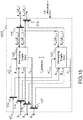
- the figure 14 describes in detail the filtering and the method of suppressing the interference.
- the concatenation block 204 simply serves to concatenate the vectors of the soft estimates x u of size MT u in a single vector x of size MT.
- the block "Generation of estimated received signals" 205 generates an estimate of the R received signals (useful part plus any interference of the type) to the receiver, concatenated in the output vector H x of size MR.
- x is a vector of zeros (no estimate available).
- the separator 206 separates the vector H x in R vectors of size M , one for each channel of the receiver.
- the concatenation blocks 210 u concatenate together the signals of the T u antennas of the same user u.
- the vector sums 211 u generate the frequency estimates (of size T u M ) of the equalized symbols by adding the estimates of the useful signals to the filtered correction signals coming from the banks of filters 208, as a generalization of the sums from the block 201 to SISO case.
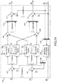
- the MU-MIMO 105T soft demodulator represented in figure 13 , Consists of flexible U demodulators MIMO separated 105T u, which separately treat the equalized signals corresponding to the same user transmission antennas.
- the scheduling and initialization manager 311 ( figure 13 ) activates all MIMO soft demodulators during self-iterations, thus generating all soft estimates x u and their corresponding average reliability v u so that the blocks implementing the interference cancel equalization functions can have signal estimates of all users.
- the scheduling manager configures only the MIMO soft demodulators of the users u ⁇ u i which must be decoded according to the current scheduling so that these demodulators calculate the extrinsic LLRs L e ( d u ) to be sent to the decoders of the interested users.
- the manager 311 will trigger the initialization of the soft demodulators MIMO 105T u according to the chosen strategy ( see description above for the MU-MIMO turbo-receiver figure 12 ).
- the soft demodulator MIMO 105T is composed of u T u flexible SISO demodulator 105 already described (see figure 5 ) which are all activated at the same time by the command from the scheduling and initialization manager 311 ( figure 13 ).
- Each flexible SISO demodulator 105 processes the data vectors corresponding to one of the transmission antennas of the user u, using its corresponding constellation ⁇ t , u .
- the separation block 113 deconcatens the vector ⁇ v , u 2 of size T u residual noise variances, in T u values ⁇ v , t , u 2 to send to the demodulators.
- the separation block 114 deconcatens the vector x u representing signals after equalization and interference suppression of size MT u , T u vectors x t, u to be sent to the demodulators.
- the separation block 115 deconcatenates the vector L a ( d u ) representing the LLRs a priori from the decoder of the user u and of size equal to the sum of the length of the packets coded on the T u antennas of the user.
- T vectors u L (d t, u) representing the a priori LLRs of the packet sent on antenna T of the user u, to be sent to the demodulators.
- the concatenation devices 116, 117, 118 operate in the opposite way to the blocks 113, 114, 105, respectively on Reliability v t, u , flexible estimates of symbols issued x t, u and extrinsic LLRs L e ( d t, u ) to form vectors v u , x u and L e ( d u ).
- a single MIMO 105T soft demodulator block u is used at the MIMO receiver, and the symbols transmitted are denoted x t , 1 , with the corresponding code word d 1 .
- the invention is also applied trivially to those skilled in the art in schemes with orthogonal block-type space-time codes, such as that of Alamouti and described for SC-FDMA in article [12] , for example. These diagrams are not represented.
- orthogonal block-type space-time codes there are detection methods known to those skilled in the art [12] with maximum likelihood or with a posterior probability maximum with reduced complexity.
- the invention described here can be applied after having adapted the calculations of the interference canceling linear equalization block 502 and the calculation block of the parameters of the receiver 503, for example as described in [12] so as to take into account counts the structure of the space-time code in blocks of orthogonal type used at the transmitter.
Landscapes
- Engineering & Computer Science (AREA)
- Power Engineering (AREA)
- Computer Networks & Wireless Communication (AREA)
- Signal Processing (AREA)
- Physics & Mathematics (AREA)
- Probability & Statistics with Applications (AREA)
- Radio Transmission System (AREA)
Abstract
L'invention concerne un procédé pour améliorer le calcul d'estimation des symboles d'un signal modulé et de la fiabilité de l'estimée, comportant au moins les étapes suivantes :• Une étape de calcul d'estimations souples (301) du signal par une technique de vraisemblance exacte ou approximée (304), en utilisant les symboles estimésdu bloc de données courant, les symboles estimés étant caractérisés par une mesure de fiabilité moyenne (302),• Une étape de division gaussienne (306) du signal estimé par par le signal estimépour générer une estimation souple du signal transmiset une variance extrinsèque (fiabilité) moyenne,• Une étape de lissage adaptatif (307) sur le signal estimé par la division gaussienne et sur les mesures de fiabilités, pour fournir une estimationdu signal transmis et une mesure de fiabilitéassociée.Récepteur obtenu par le procédé.The invention relates to a method for improving the estimation calculation of the symbols of a modulated signal and the reliability of the estimate, comprising at least the following steps: • A step of calculating flexible estimates (301) of the signal by an exact or approximated likelihood technique (304), using the estimated symbols of the current data block, the estimated symbols being characterized by a mean reliability measure (302), • A Gaussian division step (306) of the estimated signal by by the signal estimated to generate a soft estimate of the transmitted signal and an average extrinsic variance (reliability), • an adaptive smoothing step (307) on the signal estimated by the Gaussian division and on the reliability measurements, to provide an estimate of the transmitted signal and a measure of reliability associated.Receiver obtained by the method.
Description
L'invention concerne un procédé pour améliorer le calcul de l'estimation des symboles d'un signal numérique modulé et de leur fiabilité, pour toute tâche qui nécessite une telle estimation. Dans le cadre des communications numériques, elle peut être utilisée pour des récepteurs de communication sans fil, ou pour des récepteurs de communications filaires. Par exemple, l'estimation des symboles présentée ici peut être utilisée pour dériver une estimation du canal (ou de certains de ses paramètres) entre l'émetteur et le récepteur. Elle peut être utilisée pour dériver une estimation des paramètres du signal ou du récepteur comme, par exemple, le décalage d'horloge, ou l'instant de réception du signal. Elle peut être utilisée aussi pour dériver des métriques de qualité du lien, comme par exemple l'information mutuelle entre les symboles émis et ceux reçus, la fiabilité de l'estimée du signal envoyé, le rapport signal sur bruit ou signal sur bruit plus interférence. Ces métriques sont utilisées avec différentes finalités, comme l'adaptation du lien, par exemple l'adaptation des paramètres d'une chaine de transmission, ou alors à la réception pour optimiser le point de fonctionnement du récepteur ou d'un ou plusieurs de ses blocs fonctionnels internes, en choisissant les bons algorithmiques et les paramétrages les plus adaptés, en fonction de la flexibilité du récepteur même.The invention relates to a method for improving the calculation of the estimation of the symbols of a modulated digital signal and their reliability, for any task that requires such an estimate. In the context of digital communications, it can be used for wireless communication receivers, or for wired communication receivers. For example, the symbol estimation presented here can be used to derive an estimate of the channel (or some of its parameters) between the transmitter and the receiver. It can be used to derive an estimate of the signal or receiver parameters such as, for example, the clock offset, or the time of signal reception. It can also be used to derive link quality metrics, such as mutual information between the transmitted and received symbols, the reliability of the sent signal estimate, the signal-to-noise ratio or the signal-to-noise plus interference ratio. . These metrics are used for different purposes, such as the adaptation of the link, for example the adaptation of the parameters of a transmission chain, or at the reception to optimize the operating point of the receiver or one or more of its internal function blocks, choosing the right algorithms and the most appropriate settings, depending on the flexibility of the receiver itself.
L'invention concerne aussi un procédé pour supprimer des interférences au sein d'un signal reçu sur un récepteur. Elle s'applique notamment à de l'égalisation avec un récepteur adaptatif de type égaliseur à retour de décision ou DFE (Digital Feedback Equalizer) permettant une égalisation des symboles reçus.The invention also relates to a method for suppressing interference within a signal received on a receiver. It applies in particular to equalization with an adaptive receiver equalizer type feedback decision or DFE (Digital Feedback Equalizer) for equalization of symbols received.
Le domaine de l'invention est celui des systèmes de communications numériques par voie radio et entre autres les émetteurs et les récepteurs de communications multivoies, c'est-à-dire comprenant plusieurs antennes.The field of the invention is that of digital radio communication systems and, inter alia, transmitters and receivers for multichannel communications, that is to say comprising several antennas.
L'invention concerne également les systèmes multi-utilisateurs dans lesquels les ressources de communications sont partagées entre plusieurs utilisateurs qui peuvent communiquer simultanément par un partage de bandes fréquentielles ou de créneaux ou slots temporels.The invention also relates to multi-user systems in which the communication resources are shared between several users who can simultaneously communicate by sharing frequency bands or slots or time slots.
Plus généralement, l'invention concerne tous les systèmes de communication multi-utilisateurs dans lesquels de forts niveaux d'interférences sont générés à la fois entre des émetteurs associés à des utilisateurs différents mais également entre les symboles véhiculés par un signal transmis par un utilisateur du fait des perturbations inhérentes au canal de propagation.More generally, the invention relates to all multi-user communication systems in which high levels of interference are generated both between transmitters associated with different users but also between the symbols conveyed by a signal transmitted by a user of the device. makes disturbances inherent to the propagation channel.
Afin de supprimer ou au moins limiter l'interférence générée sur le signal reçu, il est connu de mettre en oeuvre un procédé de suppression d'interférence au sein du récepteur. Cette fonctionnalité a pour but de nettoyer le signal reçu des diverses sources d'interférences avant son décodage.In order to eliminate or at least limit the interference generated on the received signal, it is known to implement an interference suppression method within the receiver. This feature is intended to clean the signal received from the various sources of interference before it is decoded.
Dans ce contexte, l'invention concerne précisément le domaine de la suppression d'interférence dans un contexte multi-utilisateurs dans le cadre des récepteurs itératifs, qui consiste en l'itération des fonctions de suppression d'interférence et de décodage dans l'objectif final d'améliorer le taux d'erreur bit ou le taux d'erreur paquet sur les symboles décodés.In this context, the invention precisely relates to the field of interference suppression in a multi-user context in the context of iterative receivers, which consists in the iteration of the interference suppression and decoding functions in the objective final to improve the bit error rate or the packet error rate on the decoded symbols.
L'invention trouve entre autres son application dans les systèmes de communication cellulaires tels que le système 3GPP LTE.The invention finds inter alia its application in cellular communication systems such as the 3GPP LTE system.
L'invention vise également une méthode d'égalisation dans le domaine fréquentiel et qui soit flexible, adaptée à un contexte soit mono-utilisateur, soit multi-utilisateurs et avec un récepteur mettant en oeuvre un traitement soit non-itératif, soit itératif.The invention also aims at a method of equalization in the frequency domain and which is flexible, adapted to a single-user context, or multi-user and with a receiver implementing a treatment is non-iterative or iterative.
Un transfert d'information d'une source à une destination implique la propagation par un canal qui peut être, par exemple, un canal radio, un canal filaire (tel qu'un câble coaxial), etc. Certains moyens de propagation génèrent une interférence dite inter-symbole sur le signal reçu. Autrement dit, le signal reçu échantillonné à un instant donné, après compensation des retards de propagation et de traitement, et ayant une synchronisation correcte, ne contient pas seulement le symbole envoyé (éventuellement amplifié et avec une perturbation de phase) plus du bruit, mais un mélange ou combinaison linéaire de symboles envoyés.A transfer of information from a source to a destination involves propagation through a channel which may be, for example, a radio channel, a wired channel (such as a coaxial cable), etc. Some propagation means generate inter-symbol interference on the received signal. In other words, the received signal sampled at a given moment, after compensation of propagation delays and processing, and having a correct synchronization, not only contains the symbol sent (possibly amplified and with a phase disturbance) plus noise, but a mixture or linear combination of symbols sent.
Il est usuel dans ce cas d'utiliser des algorithmes d'égalisation pour réduire l'effet parasite de l'interférence inter-symbole (ISI). De nombreuses méthodes d'égalisation sont décrites dans l'art antérieur. L'objectif est d'atteindre des performances optimales données par la borne du filtre adapté (qui est une borne inférieure sur le taux d'erreur paquet) tout en étant facile d'utilisation. Les algorithmes doivent donc avoir une complexité de calcul, une occupation de mémoire et une latence de traitement compatibles, à la fois aux applications qui utilisent les récepteurs en question et aux contraintes des plateformes matérielles sur lesquelles ils sont implémentés. Le problème technique posé est donc de trouver des algorithmes qui trouvent un bon compromis performances/complexité d'implémentation par rapport aux applications visées.It is customary in this case to use equalization algorithms to reduce the spurious effect of intersymbol interference (ISI). Many equalization methods are described in the prior art. The goal is to achieve optimal performance given by the adapted filter terminal (which is a lower bound on the packet error rate) while being easy to use. The algorithms must therefore have computing complexity, memory occupancy and processing latency compatible, both to the applications that use the receivers in question and to the constraints of the hardware platforms on which they are implemented. The technical problem is therefore to find algorithms that find a good compromise performance / complexity of implementation with respect to the targeted applications.
Il existe plusieurs classes d'égaliseurs : les égaliseurs linéaires, les égaliseurs à retour de décision (DFE ou Decision Feedback Equalizers), les égaliseurs à effacement d'interférences (Interference Cancellation) et les détecteurs du maximum a posteriori (Maximum A Posteriori - MAP), ou des détecteurs qui estiment une séquence au maximum de vraisemblance (Maximum Likelihood Sequence Estimation - MLSE). Ces égaliseurs peuvent être déclinés en forme itérative. Des récepteurs itératifs particuliers sont les récepteurs dits « turbo », où il existe un échange réitéré d'information probabiliste extrinsèque entre blocs de traitements, par exemple entre le bloc d'égalisation et le bloc de décodage.There are several equalizer classes: linear equalizers, decision feedback equalizers (DFEs), interference canceling equalizers (Interference Cancellation), and maximum posteriori (MAP) detectors. ), or detectors that estimate a Maximum Likelihood Sequence Estimation (MLSE). These equalizers can be declined in iterative form. Particular iterative receivers are so-called "turbo" receivers, where there is a repetitive exchange of extrinsic probabilistic information between processing blocks, for example between the equalization block and the decoding block.
Dans le domaine des égaliseurs itératifs, les égaliseurs de l'état de l'art peuvent se distinguer en fonction du type de signal de retour :
- Retour dur (DFE conventionnel) ou souple à partir du démodulateur ou du décodeur de canal [13],
- Retour extrinsèque du décodeur de canal [2],
- Retour a posteriori du décodeur de canal [14].
- Hard return (conventional DFE) or soft return from the demodulator or channel decoder [13],
- Extrinsic return of the channel decoder [2],
- Retrospective return of the channel decoder [14].
Plus en détail, la structure de l'égaliseur DFE fréquentiel classique a été présentée dans la référence [13] et étendue au cas d'égaliseur fractionnel dans [8]. Ces articles présentent des égaliseurs sans boucle turbo, où le signal de retour est soit de type classique dur, soit souple et calculé avec la probabilité a posteriori sur le signal égalisé. Les égaliseurs de type fréquentiel ont été ensuite étendus pour prendre en compte un signal de retour calculé à partir de probabilités extrinsèques fournies par le décodeur, il s'agit des égaliseurs de type « turbo », voir par exemple [2]. Dans l'article [14] les auteurs montrent sur un cas de détecteur linéaire pour des systèmes multi-antennaires (on traite ici l'interférence entre antennes) qu'un signal de retour calculé à partir de probabilités a posteriori fournies par le décodeur peut améliorer les performances du système par rapport à un signal de retour calculé sur les probabilités extrinsèque. Les auteurs de l'article [12] appliquent les retours extrinsèques en provenance du décodeur à un cas de transmissions sans fil multiutilisateurs où les émetteurs sont dotés d'antennes multiples et appliquent un code espace-temps. Thomas Minka propose dans son rapport technique [3] la propagation d'espérance (Expectation Propagation - EP - en anglais), une technique de l'inférence bayésienne, qui est un algorithme itératif pour l'estimation de densité de probabilité a posteriori. Cette méthode mathématique générique peut être utilisée pour approximer la solution d'un problème de maximisation de la probabilité a posteriori ou MAP de façon itérative. La propagation d'espérance EP peut aussi être vue comme un algorithme de passage de messages connu sous l'expression anglo-saxonne « message passing », en particulier comme une généralisation de l'algorithme de propagation de croyance (Belief Propagation - BP - en anglais) aux cas de distributions de probabilité non-catégoriques mais appartenant à la famille exponentielle. En particulier, ce concept permet d'effectuer un meilleur « message passing » avec des estimateurs à erreur quadratique moyenne minimum (Minimum Mean Square Error - MMSE). Dans le domaine des communications numériques et en particulier des récepteurs turbo, le concept « d'expectation propagation » permet de calculer un type de retour souple différent. En particulier, la référence [6] utilise ce nouveau retour souple dans le cadre d'un récepteur à entrées multiples sorties multiples, (Multiple-Input Multiple-Output - MIMO), ce qui permet de mieux approcher les performances MAP. Dans le cadre de l'égalisation simple, la référence [17] étudie un signal de retour basé sur le concept de l'EP à partir du démodulateur souple, pour les égaliseurs linéaires par bloc dans le domaine temporel. La solution décrite dans [17] nécessite l'inversion de matrices qui ont potentiellement une grande taille et donc avec une complexité computationnelle et mémorielle non négligeable. Dans le cadre de la turbo-égalisation la référence [15] est une extension de la référence [17], avec ses défauts en termes de complexité. Les auteurs de [15] proposent une structure avec une double boucle (égaliseur/démodulateur, démodulateur/décodeur), qui a des performances sous-optimales puisque les auteurs négligent dans le démodulateur souple la combinaison de l'information en provenance du décodeur avec celle en provenance de l'égaliseur.In more detail, the structure of the classical frequency DFE equalizer has been presented in reference [13] and extended to the case of fractional equalizer in [8]. These articles present equalizers without turbo loop, where the return signal is either of hard conventional type, or flexible and calculated with the posterior probability on the equalized signal. Frequency type equalizers were then extended to take into account a feedback signal calculated from extrinsic probabilities provided by the decoder, these are the "turbo" type equalizers, see for example [2]. In the article [14] the authors show on a case of linear detector for multi-antennal systems (we treat here the interference between antennas) that a return signal computed from posterior probabilities provided by the decoder can improve the performance of the system with respect to a return signal calculated on the extrinsic probabilities. The authors of article [12] apply extrinsic returns from the decoder to a case of multi-user wireless transmissions where the transmitters have multiple antennas and apply a space-time code. Thomas Minka proposes in his technical report [3] Expectation Propagation (EP), a technique of Bayesian inference, which is an iterative algorithm for estimating posterior probability density. This generic mathematical method can be used to approximate the solution of a posteriori or MAP probability maximization problem iteratively. Expectancy propagation EP can also be seen as a message passing algorithm known as the "message passing", in particular as a generalization of the belief propagation algorithm (Belief Propagation - BP - in English). English) to cases of non-categorical probability distributions but belonging to the exponential family. In In particular, this concept allows for better message passing with minimum average square error (MMSE) estimators. In the field of digital communications and in particular turbo receivers, the concept of "propagation expectation" makes it possible to calculate a different type of soft return. In particular, the reference [6] uses this new soft return in the context of a multiple-input multiple-output (MIMO) receiver, which makes it possible to better approach the MAP performance. In the context of simple equalization, reference [17] studies a return signal based on the concept of PE from the soft demodulator, for block linear equalizers in the time domain. The solution described in [17] requires the inversion of matrices that potentially have a large size and therefore with considerable computational and memory complexity. As part of the turbo-equalization reference [15] is an extension of the reference [17], with its defects in terms of complexity. The authors of [15] propose a structure with a double loop (equalizer / demodulator, demodulator / decoder), which has suboptimal performances since the authors neglect in the flexible demodulator the combination of the information coming from the decoder with that from the equalizer.
La référence [16] traite de l'égalisation fréquentielle avec EP dans le cas multi-utilisateurs où les émetteurs mobiles sont équipés d'une seule antenne de transmission. Dans une des approches proposées, le retour EP est calculé sur une distribution Gaussienne coloré, c'est-à-dire, en laissant chaque symbole estimé au démodulateur avoir une mesure de fiabilité propre à lui. Cela contraint le récepteur fréquentiel à avoir une structure très complexe, nécessitant l'inversion d'une matrice pleine à chaque bloc de données. Un récepteur alternatif moins complexe est aussi dérivé, avec une hypothèse de moindres carrés, mais l'égaliseur dévient alors inutilisable dès lors que le canal de propagation présente des zéros spectraux.Reference [16] deals with frequency equalization with EP in the multi-user case where the mobile transmitters are equipped with a single transmitting antenna. In one of the approaches proposed, the return EP is calculated on a colored Gaussian distribution, that is to say, leaving each estimated symbol to the demodulator to have a measure of reliability specific to it. This forces the frequency receiver to have a very complex structure, requiring the inversion of a full matrix to each block of data. A less complex alternative receiver is also derived, with a least squares hypothesis, but the equalizer then deviates unusable when the propagation channel has spectral zeros.
Les méthodes connues de l'art antérieur ne permettent pas de prendre en compte un ou plusieurs des problèmes listés ci-après, ou encore conjointement, les aspects suivants :
- La mise en oeuvre d'une chaîne de réception numérique itérative qui inclut un récepteur adaptatif à suppression d'interférence qui transforme le canal de propagation en un canal équivalent à bruit additif Gaussien,
- Le récepteur adaptatif à suppression d'interférence est auto-itéré avec un démodulateur qui lui fournit un retour qui est une estimation du signal transmis,
- Le calcul d'un retour de type propagation d'espérance au sein du démodulateur souple, sur une distribution gaussienne blanche, c'est-à-dire où l'ensemble des symboles estimés du bloc de données est caractérisé par une seule mesure de fiabilité,
- L'utilisation d'un procédé de lissage adaptatif sur les symboles estimés par le retour EP, et sur la variance caractérisant la fiabilité ce retour. Ce procédé permet de choisir un compromis entre la robustesse des estimations et la vitesse de convergence du procédé itératif,
- L'utilisation éventuelle d'une technique de protection supplémentaire contre des estimations erronées, en remplaçant le retour EP par un retour a posteriori, suivant la valeur de la fiabilité des estimés EP.
- La mise en oeuvre d'un récepteur traitant l'interférence entre symboles dans le domaine fréquentiel,
- La mise en oeuvre d'un récepteur fractionnaire qui traite de l'égalisation fréquentielle du canal avec un facteur de sur-échantillonnage,
- La mise en oeuvre d'un récepteur fréquentiel avec recouvrement de blocs de données, où le retour EP est par ailleurs utilisé pour la réduction de l'interférence entre blocs,
- L'utilisation des retours EP au sein d'un détecteur multi-utilisateur et où les utilisateurs peuvent être équipés d'un nombre variable (une ou plusieurs) d'antennes de transmission. Le retour EP blanchi est alors utilisé pour traiter l'interférence entre utilisateurs et l'interférence multi-antennaire, en plus de l'interférence entre symboles.
- The implementation of an iterative digital reception chain which includes an interference-suppressive adaptive receiver which transforms the propagation channel into a channel equivalent to Gaussian additive noise,
- The interference canceling adaptive receiver is self-iterated with a demodulator which provides it with a feedback which is an estimate of the transmitted signal,
- The computation of a return of type propagation of expectation within the flexible demodulator, on a white Gaussian distribution, that is to say where all the estimated symbols of the data block is characterized by a single measure of reliability ,
- The use of an adaptive smoothing method on the symbols estimated by the return EP, and on the variance characterizing the reliability this return. This method makes it possible to choose a compromise between the robustness of the estimates and the speed of convergence of the iterative process,
- The possible use of an additional protection technique against erroneous estimates, by replacing the EP return with a posteriori return, depending on the reliability value of the EP estimates.
- The implementation of a receiver processing inter-symbol interference in the frequency domain,
- The implementation of a fractional receiver which deals with frequency equalization of the channel with an oversampling factor,
- The implementation of a frequency receiver with overlay of data blocks, where the return EP is also used for the reduction of interference between blocks,
- The use of EP returns within a multi-user detector and where users can be equipped with a variable number (one or more) of transmission antennas. The bleached EP return is then used to deal with user interference and multi-antenna interference, in addition to intersymbol interference.
La suite de la description fait appel aux notations suivantes :
- x dénote un scalaire;
- x dénote un vecteur;
- X dénote une matrice;
- [Xi]i=1..N est le vecteur contenant les coefficients xi;
-

- x T est le vecteur transposé de x (pareil pour les matrices);
- x * est le vecteur conjugué de x (pareil pour les matrices);
- x H est le vecteur hermitien, c'est-à-dire le vecteur transposé et conjugué, de x (pareil pour les matrices);
- x dénote la représentation en domaine fréquentielle du vecteur x ;
- X dénote la représentation en domaine fréquentielle de la matrice X ;
- tr(X) est la trace de la matrice X;
- ⊗ dénote le produit de Kronecker;
- ⊙ dénote le produit terme à terme entre deux vecteurs ( c = a ⊙ b est tel que cn = anbn), aussi appelé produit matriciel de Hadamard, ou produit de Schur ;
- circ(x) est une matrice circulante avec première colonne égale à x;
- diag(x) est une matrice diagonale avec les coefficients x sur sa diagonale;
- b : vecteur des bits d'information ;
- d : vecteur des bits codés et entrelacés ;
- [x] : espérance de x selon la distribution de probabilités


- F M : la matrice de transformée de Fourier de taille M × M, l'entrée k, l de la matrice est


- I N : matrice identité de taille NxN ;
- M : taille d'un vecteur de données à égaliser, correspondant aussi à la taille de FFT dans un émetteur de type SC-FDMA ;
- : fonction d'étiquetage binaire d'un symbole de la constellation ;

- N : taille de la IFFT dans un émetteur de type SC-FDMA, correspondant au nombre total de sous-porteuses du modulateur/démodulateur. Cela aussi est équivalent au nombre d'échantillons temporels ;
- R : nombre d'antennes de réception ;
- s : identifiant entier de l'auto-itération (
entre 0 et) ;
- : nombre d'auto-itérations du récepteur (nombre entier égal ou supérieur à zéro) pour la τ-ième turbo-itération ;

- τ : identifiant entier de la turbo-itération (
entre 0 et) ;
- : nombre de turbo-itérations du récepteur (nombre entier égal ou supérieur à zéro) ;

- Tu : nombre d'antenne de transmission de l'utilisateur u ;
- U : nombre d'utilisateurs (notamment d'émetteurs) ;
-
v : fiabilité globale de l'estimationx ; - [x] : variance de x selon la distribution de probabilité
 ,
,


- : constellation des symboles de l'utilisateur u ;

-
x : estimation du symbole transmis x fournie par le démodulateur ; - x̂ : estimation du symbole transmis x fournie par le récepteur adaptatif à suppression d'interférence ;
- Σ w : la matrice de covariance du bruit dans le domaine fréquentiel
- x denotes a scalar;
- x denotes a vector;
- X denotes a matrix;
- [X i ] i = 1..N is the vector containing the coefficients x i ;
-
- x T is the transposed vector of x (the same for matrices);
- x * is the conjugate vector of x (same for matrices);
- x H is the Hermitian vector, that is, the transposed and conjugated vector, of x (same for the matrices);
- x denotes the frequency domain representation of the vector x ;
- X denotes the frequency domain representation of the matrix X ;
- tr ( X ) is the trace of the matrix X ;
- ⊗ denotes Kronecker's product;
- ⊙ denotes the term term product between two vectors ( c = a ⊙ b is such that c n = a n b n ), also called Hadamard matrix product, or Schur product;
- circ ( x ) is a circulating matrix with first column equal to x ;
- diag ( x ) is a diagonal matrix with the coefficients x on its diagonal;
- b : vector of the information bits;
- d : vector coded and interleaved bits;
- [ x ]: expectation of x according to the probability distribution
- F M : the Fourier transform matrix of size M × M, the input k, l of the matrix is
- I N : identity matrix of size N x N ;
- M : size of a data vector to be equalized, also corresponding to the size of FFT in a transmitter of SC-FDMA type;
- : binary tagging function of a constellation symbol;
- N : size of the IFFT in an SC-FDMA transmitter, corresponding to the total number of subcarriers of the modulator / demodulator. This too is equivalent to the number of temporal samples;
- R : number of receiving antennas;
- s : integer identifier of the auto-iteration (between 0 and );
- : number of self-iterations of the receiver (integer equal to or greater than zero) for the τ- th turbo-iteration;
- τ : integer identifier of the turbo-iteration (between 0 and );
- : number of turbo-iterations of the receiver (integer equal to or greater than zero);
- T u : number of transmission antenna of the user u ;
- U : number of users (including transmitters);
-
v : overall reliability of the estimatex ; - [ x ]: variance of x according to the probability distribution,
- : constellation of user symbols u ;
-
x : estimation of transmitted symbol x provided by the demodulator; - x : estimation of the transmitted symbol x provided by the adaptive interference suppression receiver;
- Σ w : the frequency covariance matrix in the frequency domain
Dans la suite de la description l'expression « division gaussienne » fait référence à une division entre deux fonctions de densité de probabilité gaussiennes, avec une « normalisation » de la fonction résultante afin que cette dernière soit encore une fonction de densité de probabilité gaussienne. Pour décrire cette opération dans le cas gaussien, il suffit de calculer la moyenne et la variance de la densité de probabilité résultante à partir des moyennes et variances des deux densités de probabilité considérées.In the rest of the description, the expression "Gaussian division" refers to a division between two Gaussian probability density functions, with a "normalization" of the resulting function so that the latter function is still a Gaussian probability density function. To describe this operation in the Gaussian case, it is sufficient to calculate the mean and the variance of the resulting probability density from the means and variances of the two probability densities considered.
L'invention concerne un procédé pour améliorer l'estimation des symboles d'un signal modulé et de la fiabilité de l'estimée, le signal comprenant un ou plusieurs blocs de données, comportant au moins les étapes suivantes exécutées au niveau d'un processeur :
- Une étape de calcul d'estimations souples du signal qui calcule les symboles estimés


γ (τ,s), - Une étape de division gaussienne du signal estimé


v ' (τ,s+1) avec:

- Une étape de lissage adaptatif sur le signal estimé par la division gaussienne et sur les mesures de fiabilités, pour fournir une estimation
x (τ,s+1) du signal transmis et une mesure de fiabilitév (τ,s+1) associée.
- A step of calculating flexible estimates of the signal which calculates the estimated symbols
reliability γ ( τ, s ) , - A step of Gaussian division of the estimated signal
v ' ( τ, s +1) with: - An adaptive smoothing step on the signal estimated by the Gaussian division and on reliability measures, to provide an estimate
x ( τ, s +1) of the transmitted signal and a measure of reliabilityv ( τ, s +1) associated.
Selon une variante de réalisation, on calcule une estimation souple du signal transmis ![]()
![]()
![]()
- Une étape de calcul de distributions a priori du signal transmis à partir d'entrées/sorties souples binaires,
- Une étape de calcul d'estimations souples du signal transmis en utilisant en entrée des distributions de probabilité a posteriori, calculées à partir des vraisemblances gaussienne du signal estimé x̂ (τ,s) et les distributions a priori calculées à l'étape précédente, ladite estimation est caractérisée par une mesure de fiabilité moyenne
γ (τ,s).
- A step of calculating a priori distributions of the signal transmitted from binary soft I / Os,
- A step of calculating flexible estimates of the transmitted signal by using, in input, posterior probability distributions, calculated from the Gaussian likelihoods of the estimated signal x ( τ, s ) and the prior distributions calculated in the preceding step, said estimate is characterized by a measure of average reliability
γ ( τ, s ) .
Le procédé peut aussi comporter :
- Une étape de décodage par un décodeur binaire à entrées/sorties souples,
- Une étape d'initialisation du démodulateur souple, en calculant une estimation a priori du signal transmis, ladite estimation étant caractérisée par une fiabilité moyenne
v (τ,0), - Lesdites valeurs d'estimation a priori et de fiabilité moyenne calculée représentant des valeurs de sortie et/ou étant utilisées pour initialiser l'étape de lissage adaptatif.
- A step of decoding by a binary decoder with flexible inputs / outputs,
- A step of initialization of the flexible demodulator, by calculating a prior estimate of the transmitted signal, said estimate being characterized by an average reliability
v ( τ, 0) , - Said a priori estimate and calculated mean reliability values representing output values and / or being used to initialize the adaptive smoothing step.
Selon une variante de réalisation, le procédé comprend en outre une étape de désentrelacement et d'entrelacement des informations souples sur le signal transmis, lors de l'échange itératif entre un démodulateur souple et un décodeur binaire à entrées/sorties souples.According to an alternative embodiment, the method further comprises a step of deinterleaving and interleaving the soft information on the transmitted signal, during the iterative exchange between a soft demodulator and a soft input / output binary decoder.
Le procédé est utilisé pour la suppression d'interférence au sein d'un signal issu d'au moins un émetteur reçu sur un récepteur comprenant une ou plusieurs antennes, ledit signal comprenant un ou plusieurs blocs de données et comporte en outre les étapes suivantes :
- Une étape de calcul des paramètres du récepteur, en utilisant la connaissance du canal,
- Une étape de traitement du signal reçu par un récepteur à suppression d'interférence qui génère une autre estimation x̂ (τ,s) du signal transmis en utilisant une estimation préalable
x̂ (τ,s+1) du signal transmis x et la connaissance du canal, l'estimation du signal étant effectuée par le récepteur à suppression d'interférence, - Le calcul de la fiabilité
- Une étape d'échange itératif des estimations du signal transmis, entre le récepteur à suppression d'interférence et le démodulateur souple,
- Une étape de calcul d'information souple sur les bits du signal transmis, faite à partir du signal démodulé.
- A step of calculating the parameters of the receiver, using the knowledge of the channel,
- A step of processing the signal received by an interference suppression receiver that generates another estimate x ( τ, s ) of the transmitted signal using a prior estimate
x ( τ, s +1) of the transmitted signal x and the knowledge of the channel, the estimation of the signal being carried out by the interference suppression receiver, - The calculation of
reliability - An iterative exchange step of the estimates of the transmitted signal, between the interference suppression receiver and the soft demodulator,
- A step of computing soft information on the bits of the transmitted signal, made from the demodulated signal.
Le procédé peut aussi comporter les étapes suivantes :
- Une étape de calcul des paramètres du récepteur adaptatif, en utilisant la connaissance du canal et la fiabilité des retours souples du démodulateur,
- Une étape d'échange itératif des fiabilités des estimations du signal transmis entre le bloc qui calcule les paramètres du récepteur adaptatif et le démodulateur souple.
- A step of calculating the parameters of the adaptive receiver, using the knowledge of the channel and the reliability of the soft returns of the demodulator,
- A step of iterative exchange of the reliability of the estimates of the signal transmitted between the block which calculates the parameters of the adaptive receiver and the flexible demodulator.
Selon une variante de réalisation, le procédé pour supprimer l'interférence au niveau d'un signal comporte les étapes suivantes :
- Une étape d'estimation des paramètres du canal entre l'émetteur et le récepteur en utilisant le signal reçu,
- Une étape de calcul des paramètres du récepteur adaptatif ou non, en utilisant l'estimation des paramètres du canal et la fiabilité des retours souples du démodulateur,
- Une étape d'échange itératif des fiabilités des estimations du signal transmis entre le bloc qui calcule les paramètres du récepteur adaptatif et le démodulateur souple.
- A step of estimating the channel parameters between the transmitter and the receiver using the received signal,
- A step of calculating the parameters of the adaptive receiver or not, by using the estimation of the parameters of the channel and the reliability of the soft returns of the demodulator,
- A step of iterative exchange of the reliability of the estimates of the signal transmitted between the block which calculates the parameters of the adaptive receiver and the flexible demodulator.
Le procédé peut comprendre en outre une étape itérative d'estimation des paramètres du canal, en utilisant l'estimation souple du signal transmis et sa fiabilité en provenance du démodulateur souple, conjointement avec le signal reçu.The method may further include an iterative step of estimating channel parameters, using the soft estimate of the transmitted signal and its reliability from the soft demodulator together with the received signal.
L'étape de traitement du signal reçu par un récepteur à suppression d'interférence et l'étape de calcul de ses paramètres comprennent, par exemple:
- Une étape de conversion du signal reçu dans le domaine fréquentiel,
- Une étape de calcul des paramètres de l'égaliseur dans le domaine fréquentiel, qui réalise les fonctions du bloc,
- Une étape d'égalisation linéaire à suppression d'interférence dans le domaine fréquentiel, paramétrée selon les sorties obtenues lors du calcul des paramètres de l'égaliseur dans le domaine fréquentiel,
- Une étape de conversion du signal traité dans le domaine temporel,
- Une étape de conversion dans le domaine fréquentiel de l'estimation souple du signal transmis fournie par le démodulateur souple.
- A step of converting the received signal into the frequency domain,
- A step of calculating the parameters of the equalizer in the frequency domain, which realizes the functions of the block,
- A frequency-canceling linear equalization step in the frequency domain, parameterized according to the outputs obtained during the calculation of the parameters of the equalizer in the frequency domain,
- A step of converting the processed signal into the time domain,
- A conversion step in the frequency domain of the soft estimation of the transmitted signal provided by the flexible demodulator.
L'étape de traitement du signal reçu par un récepteur à suppression d'interférence et l'étape de calcul de ses paramètres comprennent, par exemple:
- Une étape de séparation du signal reçu y en P segments y p de Np symboles chacun, avec recouvrement, p = 1, ..., P.
- Une étape de conversion de chacun de segments du signal reçu dans le domaine fréquentiel,
- Une étape du calcul des paramètres des P égaliseurs dans le domaine fréquentiel, qui réalise les fonctions du bloc,
- Une étape d'égalisation linéaire à suppression d'interférence dans le domaine fréquentiel de chacun des segments, paramétrée selon les sorties obtenues lors du calcul des paramètres des P égaliseurs dans le domaine fréquentiel,
- Une étape de conversion de chacun des signaux traités dans le domaine temporel, et d'extraction des symboles non recouverts pour obtenir une estimation x̂ ,
- Une étape de conversion dans le domaine fréquentiel de l'estimation souple du signal transmis fournie par le démodulateur souple.
- A step of separating the received signal y into P segments y p of N p symbols each, with overlap, p = 1, ..., P.
- A step of converting each of the segments of the received signal into the frequency domain,
- A step of the calculation of the parameters of the P equalizers in the frequency domain, which realizes the functions of the block,
- A step of linear equalization with interference suppression in the frequency domain of each of the segments, parameterized according to the outputs obtained during the calculation of the parameters of the P equalizers in the frequency domain,
- A step of converting each of the processed signals in the time domain, and extracting the uncoated symbols to obtain an estimate x ,
- A conversion step in the frequency domain of the soft estimation of the transmitted signal provided by the flexible demodulator.
Le calcul des paramètres des P égaliseurs dans le domaine fréquentiel peut utiliser la connaissance de la statistique de l'interférence entre segments, estimée à partir de la fiabilité des retours du démodulateur souple.The computation of the parameters of the P equalizers in the frequency domain can use the knowledge of the statistics of the interference between segments, estimated from the reliability of the returns of the soft demodulator.
L'interférence résiduelle entre segments est régénérée, par exemple, en utilisant les retours du démodulateur souple, et soustraite de chacun des P segments y p , avant l'étape de conversion dans le domaine fréquentiel.Residual interference between segments is regenerated, for example, using the returns of the soft demodulator, and subtracted from each of the P segments y p , before the step of conversion in the frequency domain.
Selon un mode de réalisation l'étape de traitement du signal reçu par un récepteur à suppression d'interférence et l'étape de calcul de ses paramètres comprennent:
- Un sur-échantillonnage du signal reçu avec un facteur de sur-échantillonnage o,
- Une étape de conversion en fréquence du signal reçu suréchantillonné,
- Une étape de calcul du filtre de l'égaliseur dans le domaine fréquentiel suréchantillonné,
- Une étape d'égalisation linéaire à suppression d'interférence dans le domaine fréquentiel suréchantillonné selon la sortie obtenue lors du calcul des paramètres de l'égaliseur dans le domaine fréquentiel suréchantillonné,
- Une étape de conversion du signal traité dans le domaine temporel, suivi d'un échantillonneur de facteur d'échantillonnage o égal au facteur de sur-échantillonnage du signal reçu.
- Une étape d'interpolation idéale de l'estimation souple du signal transmis fournie par le démodulateur souple par un facteur de suréchantillonnage o égal à celui du signal reçu (cela consiste en l'ajout de o - 1 zéros entre deux échantillons), suivi d'une conversion dans le domaine fréquentiel suréchantillonné.
- Over-sampling of the received signal with an oversampling factor o,
- A step of frequency conversion of the oversampled received signal,
- A step of calculating the equalizer filter in the oversampled frequency domain,
- A frequency-canceling linear equalization step in the oversampled frequency domain according to the output obtained during the calculating the parameters of the equalizer in the oversampled frequency domain,
- A step of converting the processed signal into the time domain, followed by a sampling factor sampler o equal to the oversampling factor of the received signal.
- An ideal interpolation step of the soft estimation of the transmitted signal provided by the flexible demodulator by an oversampling factor o equal to that of the received signal (this consists in adding o - 1 zeros between two samples), followed by an oversampled frequency domain conversion.
Le procédé est utilisé pour supprimer des interférences au sein d'un signal reçu sur un récepteur de type SC-FDMA ou SS-SC-FDMA comprenant une étape de mise en trame utilisant respectivement une modulation SC-FDMA ou SS-SC-FDMA et une étape d'exécution du procédé selon l'invention.The method is used to suppress interference within a signal received on an SC-FDMA or SS-SC-FDMA receiver comprising a framing step using respectively SC-FDMA or SS-SC-FDMA modulation and a step of executing the method according to the invention.
Le procédé peut aussi être utilisé pour supprimer des interférences au sein d'un signal reçu sur un récepteur de type SC ou SS-SC comprenant une étape de mise en trame utilisant respectivement une modulation SC ou SS-SC et une étape d'exécution du procédé selon l'invention.The method can also be used to suppress interference within a signal received on an SC or SS-SC type receiver comprising a framing step respectively using an SC or SS-SC modulation and a step of executing the process according to the invention.
L'invention concerne aussi un procédé pour supprimer des interférences au sein d'un signal reçu sur un récepteur de type OFDM ou OFDMA comprenant une étape de mise en trame utilisant respectivement une modulation OFDM ou OFDMA et une étape d'exécution du procédé selon l'invention dans lequel, l'étape de traitement du signal reçu par un récepteur à suppression d'interférence et l'étape de calcul de ses paramètres comprennent:
- Une étape de conversion du signal reçu dans le domaine fréquentiel,
- Une étape de calcul des paramètres de l'égaliseur dans le domaine fréquentiel, qui réalise les fonctions du bloc,
- Une étape d'égalisation linéaire à suppression d'interférence dans le domaine fréquentiel, paramétrée selon les sorties obtenues lors du calcul des paramètres de l'égaliseur dans le domaine fréquentiel.
- A step of converting the received signal into the frequency domain,
- A step of calculating the parameters of the equalizer in the frequency domain, which realizes the functions of the block,
- A step of linear equalization with suppression of interference in the frequency domain, parameterized according to the outputs obtained during the calculation of the parameters of the equalizer in the frequency domain.
Selon une variante, le procédé de suppression d'interférence comprend en outre:
- Une étape de génération du signal à l'émetteur selon un code espace-temps par blocs de type Alamouti ou autre code espace-temps par bloc de type orthogonal,
- Une étape d'estimation des paramètres des canaux entre les antennes de l'émetteur et celles du récepteur,
- Une étape du calcul des paramètres du récepteur dans le domaine fréquentiel, qui prennent en compte la structure du code espace-temps par blocs utilisé,
- Une étape d'égalisation linéaire à suppression d'interférence dans le domaine fréquentiel en utilisant les filtres obtenus lors du calcul des paramètres des égaliseurs dans le domaine fréquentiel, et qui combine les signaux reçus en entrée selon la méthode associé au code espace-temps par blocs utilisé par l'émetteur.
- A step of generating the signal at the transmitter according to a space-time code by Alamouti type blocks or other space-time code by orthogonal type block,
- A step of estimating the parameters of the channels between the antennas of the transmitter and those of the receiver,
- A step of the calculation of the parameters of the receiver in the frequency domain, which take into account the structure of the space-time block code used,
- A linear equalization step with interference suppression in the frequency domain using the filters obtained during the calculation of the parameters of the equalizers in the frequency domain, and which combines the signals received at the input according to the method associated with the space-time code by blocks used by the transmitter.
L'invention concerne aussi un procédé pour supprimer des interférences au sein des signaux issus d'un émetteur reçus sur un récepteur, dans un réseau de type MIMO où l'émetteur est doté de plusieurs antennes de transmissions et d'un entrelaceur qui répartit les bits codés sur les antennes disponibles, comprenant une étape d'exécution du procédé selon l'invention comprenant en outre :
- Une étape de traitement des signaux reçus en provenance des antennes de l'émetteur par un récepteur à suppression d'interférence, qui en utilisant ses paramètres et une estimation préalable des signaux transmis x̂ t par les antennes d'émission t = 1, ..., T 1, de l'utilisateur génère une autre estimation des signaux émis x̂ t,
- Une étape du calcul des paramètres du récepteur qui prend en compte la présence de plusieurs antennes d'émission et les estimations des paramètres des canaux entre les antennes de l'émetteur et du récepteur,
- Une étape de démodulation souple où l'estimation du signal de chaque antenne d'émission est traitée indépendamment.
- A step of processing the signals received from the transmitter's antennas by an interference suppression receiver, which by using its parameters and a prior estimation of the transmitted signals x t by the transmitting antennas t = 1, .. ., T 1 , of the user generates another estimate of the transmitted signals x t ,
- A step of calculating the parameters of the receiver which takes into account the presence of several transmitting antennas and the estimations of the parameters of the channels between the antennas of the transmitter and the receiver,
- A soft demodulation step where the signal estimate of each transmit antenna is processed independently.
L'invention concerne aussi un procédé pour supprimer des interférences au sein des signaux issus de plusieurs émetteurs reçus sur un récepteur, dans un réseau de type MU-MIMO où les émetteurs sont dotés d'une ou plusieurs antennes de transmissions et d'un entrelaceur qui répartit les bits codés sur les antennes disponibles, comprenant une étape d'exécution du procédé selon l'invention comprenant:
- Une étape de traitement des signaux reçus en provenance des émetteurs par un récepteur à suppression d'interférence, qui en utilisant ses paramètres et une estimation préalable des signaux transmis
x t,u par les antennes d'émission t = 1, ..., Tu des utilisateurs= 1, ..., U, génère une autre estimation des signaux émis x̂ t,u, - Une étape du calcul des paramètres du récepteur qui prend en compte la présence de plusieurs utilisateurs, éventuellement avec plusieurs antennes d'émission, et d'éventuelles estimations des paramètres des canaux entre les antennes des émetteurs et du récepteur,
- Une étape de démodulation souple où l'estimation du signal de chaque antenne d'émission de chaque utilisateur est traitée indépendamment,
- Une étape d'ordonnancement des utilisateurs à décoder selon un critère basé sur la puissance des signaux reçus, ou selon une métrique dérivée de la puissance des signaux reçus et de la fiabilité de leurs constellations, ou encore selon une métrique basée sur les écarts de puissances et fiabilité entre couples d'utilisateurs.
- A step of processing the signals received from the transmitters by an interference suppression receiver, which by using its parameters and a preliminary estimate of the transmitted signals
x t, u by the transmit antennas t = 1, ..., T u of the users = 1, ..., U, generate another estimate of the transmitted signals x t, u , - A step of calculating the parameters of the receiver which takes into account the presence of several users, possibly with several transmitting antennas, and possible estimations of the parameters of the channels between the antennas of the transmitters and the receiver,
- A soft demodulation step where the signal estimation of each transmitting antenna of each user is processed independently,
- A step of scheduling users to be decoded according to a criterion based on the power of the signals received, or according to a metric derived from the power of the signals received and the reliability of their constellations, or according to a metric based on the power differences and reliability between user pairs.
L'invention concerne aussi un récepteur comportant au moins une antenne pour recevoir un signal émis par au moins un émetteur caractérisé en ce qu'il comporte au moins :
- Un processeur configuré pour exécuter le procédé d'amélioration de calcul des symboles et leurs fiabilités selon l'invention, lesdits symboles étant utilisés pour la modulation d'un signal,
- Un module de calcul des vraisemblances gaussiennes ayant une sortie reliée à un bloc de normalisation, dont la sortie est reliée à un deuxième module d'estimations souples,
- Un deuxième module d'estimations souples transmettant ses estimés


γ (τ,s) est reliée au module de division gaussienne, - Un module de lissage adaptatif relié au module de division gaussienne et fournissant les estimés souples lissées
x (τ,s+1) ainsi que leurs variancesv (τ,s+1).
- A processor configured to perform the method of improving calculation of symbols and their reliability according to the invention, said symbols being used for the modulation of a signal,
- A Gaussian likelihood calculation module having an output connected to a normalization block, the output of which is connected to a second module of flexible estimates,
- A second module of soft estimates conveying its estimates
γ ( τ, s ) is connected to the Gaussian division module, - An adaptive smoothing module connected to the Gaussian division module and providing soft smoothed estimates
x ( τ, s +1) and their variancesv ( τ, s +1) .
Le récepteur peut comporter un démodulateur souple comprenant au moins les éléments suivants :
- Un module de calcul des distributions a priori, ayant en entrée des rapports de vraisemblance LLR a priori et ayant une sortie reliée à un module de calcul de distributions a posteriori et au module de calcul d'estimations souples,
- Un deuxième module de calcul d'estimations souples, fournissant des estimés souples a priori
x (τ,0) caractérisées par une fiabilité moyennev (τ,0).
- A module for calculating prior distributions, having as input LLR likelihood ratios a priori and having an output connected to a module for calculating posterior distributions and to the module for calculating flexible estimates,
- A second module for calculating flexible estimates, providing flexible estimates a priori
x ( τ, 0) characterized by medium reliabilityv ( τ , 0) .
Le récepteur peut aussi comporter :
- Un module de sélection configuré pour sélectionner les estimés souples a priori
x (τ+0) et leur variance, ou les estimés souples lisséesx (τ,s+1) et leur variance en fonction du fait s'il s'agit ou pas de la première exécution (exécution d'initialisation) du démodulateur souple ayant en entrée du démodulateur souple les valeurs des rapports de vraisemblance LLRs a priori correspondantes aux estimées souples a priorix (τ,0).
- A selection module configured to select flexible estimates a priori
x ( τ +0) and their variance, or the soft smoothed estimatesx ( τ, s +1) and their variance depending on whether or not it is the first execution (initialization execution) of the flexible demodulator having, at the input of the soft demodulator, the values of the likelihood ratios LLRs a priori corresponding to the flexible estimates a priorix ( τ, 0) .
D'autres caractéristiques et avantages de la présente invention apparaîtront mieux à la lecture de la description d'exemples de réalisation donnés à titre illustratif et non limitatif annexée des figures qui représentent :
-
Figure 1 , une vue du système mono-utilisateur avec émetteur et récepteur utilisant une seule antenne, SISO, -
Figure 2 , un schéma-bloc avec une vue fonctionnelle d'un émetteur mono-antennaire, -
Figure 3 , un schéma de la structure d'un turbo DFE dans le cas SISO, pour un système SC-FDMA, -
Figure 4 , une structure d'égaliseur linéaire à suppression d'interférence, -
Figure 5 , une structure du démodulateur souple, -
Figure 6 etfigure 7 des courbes de performances obtenues dans le cas SISO, -
Figure 8 , un schéma généralisant le récepteur turbo DFE à des modulations quelconques, -
Figure 9 , une vue du système multi-utilisateurs, -
Figure 10 , une vue d'un système multi-utilisateurs MIMO, -
Figure 11 , un schéma bloc fonctionnel pour un émetteur multi-antennaire, -
Figure 12 , un schéma de structure d'un turbo DFE dans le cas MU-MIMO, pour un système SC-FDMA, -
Figure 13 , un démodulateur souple pour le cas MU-MIMO, -
Figure 14 , le filtrage et le procédé de suppression des interférences dans le cas MU-MIMO, et -
Figure 15 , un détail d'un bloc pour le démodulateur souple.
-
Figure 1 , a view of the single-user system with transmitter and receiver using a single antenna, SISO, -
Figure 2 , a block diagram with a functional view of a single-antenna transmitter, -
Figure 3 , a diagram of the structure of a DFE turbo in the SISO case, for an SC-FDMA system, -
Figure 4 , a linear equalizer structure with interference suppression, -
Figure 5 , a structure of the flexible demodulator, -
Figure 6 andfigure 7 performance curves obtained in the SISO case, -
Figure 8 , a scheme generalizing the turbo receiver DFE to any modulations, -
Figure 9 , a view of the multi-user system, -
Figure 10 , a view of a multi-user MIMO system, -
Figure 11 , a functional block diagram for a multi-antenna transmitter, -
Figure 12 , a structure diagram of a DFE turbo in the case MU-MIMO, for an SC-FDMA system, -
Figure 13 , a flexible demodulator for the MU-MIMO case, -
Figure 14 , the filtering and the method of suppressing interference in the MU-MIMO case, and -
Figure 15 , a detail of a block for the soft demodulator.
La technique de turbo égalisation consiste en l'itération entre la fonction d'égalisation, de démodulation souple (ici appelé aussi demapper ou demapping souple) et de décodage, généralement avec la finalité d'améliorer le taux d'erreur bit (Bit Error Rate - BER) ou le taux d'erreur paquet (Packet Error Rate - PER) tout en maitrisant la complexité du récepteur.The turbo equalization technique consists in the iteration between the function of equalization, of soft demodulation (here also called demapper or soft demapping) and decoding, generally with the aim of improving the bit error rate (Bit Error Rate - BER) or the Packet Error Rate (PER) while controlling the complexity of the receiver.
Afin de bien faire comprendre l'invention, la première variante de réalisation est donnée, à titre d'exemple non limitatif, dans le cas d'un système simple entrée simple sortie ou SISO (Single Input Single Output) illustré à la
L'émetteur mono-antennaire générique 10 pour l'application SISO est représenté en ![]()
![]()
Le bloc de mise en trame 14 peut utiliser une modulation à multiplexage par répartition orthogonale de la fréquence (Orthogonal Frequency Division Multiplexing -OFDM) avec un total de N sous-porteuses dont M sous-porteuses utilisées avec un préfixe cyclique (Cyclic Prefix - CP) et éventuellement un suffixe cyclique (Cyclic Suffix - CS). Le bloc de mise en trame peut aussi mettre en place une modulation OFDM à accès multiple, appelée dans la littérature OFDMA. Le bloc de mise en trame peut aussi mettre en place une modulation mono-porteuse à accès multiple par répartition en fréquence Single Carrier-Frequency Division Multiple Access (SC-FDMA), avec M le nombre de sous-porteuses utilisées pour le précodage avec une transformée de Fourier discrète (Discrete Fourier Transform - DFT). Ici aussi le CP et éventuellement le CS sont utilisés. Dans ce cadre, si N = M, l'émetteur implémente un signal mono-porteuse (Single Carrier - SC).The framing
Les CP et CS peuvent être substitués par une séquence constante (par exemple des zéros, ou des séquences pilotes) ou évoluant d'une trame à l'autre (par exemple par un procédé pseudo-aléatoire connu des utilisateurs), ce qui permet d'obtenir encore un signal avec la bonne propriété de périodicité partielle sur les blocs de données étendus avec l'une de ces séquences. Il est aussi possible de considérer l'utilisation d'une modulation monoporteuse avec une mise-en-forme spectrale (Spectrally Shaped - Single Carrier - SS-SC) ou une modulation mono-porteuse avec une mise-en-forme spectrale à accès multiple par répartition en fréquence (Spectrally Shaped - Single Carrier - Frequency Division Multiple Access - SS-SC-FDMA), où le signal pourrait être filtré en temps, ou en fréquence, par un filtre de mise-en-forme, après l'ajout des CP/CS.The CPs and CSs can be substituted by a constant sequence (for example zeros, or pilot sequences) or evolving from one frame to another (for example by a pseudo-random method known to the users), which makes it possible to to still obtain a signal with the good property of partial periodicity on the extended data blocks with one of these sequences. It is also possible to consider the use of single-carrier modulation with Spectrally Shaped Single Carrier (SS-SC) or mono-carrier modulation with multi-access spectral shaping Frequency Division Multiple Access (SS-SC-FDMA), where the signal could be filtered in time, or in frequency, by a filter of formatting, after the addition CP / CS.
Sans sortir du cadre de l'invention, il est possible d'utiliser des constellations ayant une propriété de non-circularité (appelée aussi impropriété dans la littérature [1]. La non-circularité s'exprime formellement par le fait que si x(n) est un symbole aléatoire de la constellation émis au temps n, alors l'espérance du symbole au carré est différente de zéro E[x 2(n)] ≠ 0. La quantité E[x 2(n)] est appelée aussi pseudo-covariance dans la littérature. Cette propriété s'étend aux signaux échantillonnés ou continus aussi. L'invention s'applique donc à des émetteurs utilisant des constellations complexes comme la modulation d'amplitude en quadrature (Quadrature Amplitude Modulation - QAM), la modulation par changement de phase ou Phase Shift Keying (PSK), la modulation par changement de phase et d'amplitude (Amplitude Phase Shift Keying - APSK) ; des constellations réelles, comme la modulation par changement de phase binaire ou « Binary Phase Shift Keying » (BPSK), ou les modulations en amplitude d'impulsion (Pulse Amplitude Modulation - PAM). La technique peut être appliquée aussi à des constellations tournées périodiquement comme la π/2-BPSK, où sur les symboles pairs on utilise une constellation BPSK classique {+1, -1} et sur les symboles impairs on utilise une constellation tournée de π/2 radians {+j, - j}, et plus généralement les constellations π/M-MPSK, où la rotation périodique est de π/M radians. Il est aussi possible d'appliquer la technique décrite ici à des constellations appelées quasi-rectilignes, c'est-à-dire des constellations dont les symboles peuvent être obtenus par filtrage complexe d'un signal décrit par les symboles d'une constellation réelle. Des exemples sont la modulation par déplacement de fréquence minimum (Minimum Shift Keying - MSK), la modulation par déplacement de fréquence minimum gaussien (Gaussian Minimum Shift Keying - GMSK), les modulations de phase continues (Continuous Phase Modulation - CPM) avec alphabet binaire ou la modulation d'amplitude en quadrature décalée en quadrature (Offset Quadrature Amplitude Modulation - OQAM).Without departing from the scope of the invention, it is possible to use constellations having a property of non-circularity (also called impropriety in the literature [1].) Non-circularity is expressed formally by the fact that if x ( n ) is a random symbol of the constellation emitted at time n, then the expectation of the squared symbol is different from zero E [ x 2 ( n )] ≠ 0. The quantity E [ x 2 ( n )] is also called pseudo-covariance in the literature This property extends to sampled or continuous signals as well. The invention thus applies to transmitters using complex constellations such as quadrature amplitude modulation (QAM), phase shift keying (PSK), phase change modulation and amplitude (Amplitude Phase Shift Keying - APSK); real constellations, such as Binary Phase Shift Keying (BPSK), or Pulse Amplitude Modulation (PAM). The technique can also be applied to periodically rotated constellations like the π / 2-BPSK, where on the even symbols we use a classical BPSK constellation {+1, -1} and on the odd symbols we use a rotated constellation of π / 2 radians {+ j, - j}, and more generally constellations π / MM PSK, where the periodic rotation is π / M radians. It is also possible to apply the technique described here to constellations called quasi-rectilinear, that is to say constellations whose symbols can be obtained by complex filtering of a signal described by the symbols of a real constellation . Examples are Minimum Shift Keying (MSK) modulation, Gaussian Minimum Shift Keying (GMSK) modulation, Continuous Phase Modulation (CPM) with binary alphabet or quadrature quadrature amplitude modulation (Offset Quadrature Amplitude Modulation - OQAM).
La
Le récepteur selon l'invention contient deux boucles de rétroaction. La première boucle est positionnée entre l'égaliseur DFE 108 et le démodulateur souple SISO 105. Dans la suite, le parcours de cette boucle est appelé « auto-itération » et un égaliseur qui utilise cette boucle est un « égaliseur auto-itéré ». La deuxième boucle se situe entre le démodulateur souple SISO 105 et le décodeur bloc « décodage » 111. Dans la suite, le parcours de cette boucle est désigné sous l'expression « turbo-itération » et un égaliseur qui utilise cette boucle est un « égaliseur turbo-itéré » ou un « turbo-égaliseur ».The receiver according to the invention contains two feedback loops. The first loop is positioned between the
Le récepteur 20 effectue un nombre
![]()
![]()
![]()
![]()
![]()
![]()
![]()
![]()
![]()
![]()
![]()
![]()
![]()
![]()
Dans la suite de la description, les paramètres en entrée ou en sortie du turbo égaliseur, du calcul égaliseur et les paramètres du démodulateur souple, et du démodulateur souple, à l'exception des observations initiales et estimations initiales y, H , Σ w , dépendent de l'identifiant de la turbo-itération courante
![]()
![]()
![]()
![]()
De plus, il convient d'initialiser les blocs au début du traitement de réception et au début de chaque turbo-itération, donc pour chaque
![]()
![]()
![]()
![]()
Dans cet exemple, la description est donnée pour un cas SC-FDMA, en sachant que les adaptations pour les autres cas cités précédemment peuvent être déduites par un homme du métier.In this example, the description is given for an SC-FDMA case, knowing that the adaptations for the other cases mentioned above can be deduced by a person skilled in the art.
Après avoir extrait les blocs de données en provenance de l'antenne de réception Ar du récepteur, à travers la suppression du CP dans le cas des systèmes SC avec CP ou du SC-FDMA, 101, les blocs de données passent à travers une transformation de Fourier rapide 102 (Fast Fourier Transform - FFT) de taille N (passage dans le domaine fréquentiel). Le signal en sortie de la FFT passe ensuite dans un bloc « De-alloc sous-p » 103 qui permet d'accéder aux M ressources fréquentielles (sous-porteuses) parmi N, à travers lesquelles le signal a été transmis. Ce bloc sélectionne seulement les sous-porteuses sur lesquelles le signal a été transmis (dé-allocation des sous-porteuses), et en sortie de ce dernier bloc de dé-allocation 103 le signal est représenté par un vecteur y de taille M, regroupant les sous-porteuses utilisés.After extracting the data blocks from the receiving antenna A r of the receiver, by deleting the CP in the case of SC systems with CP or SC-FDMA, 101, the data blocks pass through a Fast Fourier Transform (FFT) of size N (frequency domain transition). The signal at the output of the FFT then goes into a block "De-alloc sub-p" 103 which makes it possible to access the M frequency resources (sub-carriers) among N, through which the signal has been transmitted. This block selects only the sub-carriers on which the signal has been transmitted (de-allocation of the sub-carriers), and at the output of this last dis-
En parallèle, les séquences pilotes sont extraites des signaux provenant de l'antenne de réception Ar et envoyées dans le bloc « Estimation des canaux et de la variance du bruit » 104. Elles sont utilisées pour calculer une estimation de la réponse fréquentielle du canal entre l'émetteur et le récepteur, sur les M sous-porteuses d'intérêts (celles utilisées par l'utilisateur pour envoyer l'information). La réponse fréquentielle du canal entre l'émetteur et le récepteur est organisée dans un vecteur h de taille M, ou de façon équivalente, dans une matrice diagonale H = diag( h ) de taille M x M. Le bloc « Estimation des canaux et de la variance du bruit » 104 fournit aussi une estimation de la variance du bruit. Ce bruit contient la contribution du bruit thermique sur l'antenne de réception Ar et d'éventuelles interférences dues à plusieurs effets parasites en provenance soit de traitements numériques, soit d'autres signaux extérieurs. Le bloc « Estimation des canaux et de la variance du bruit » fournit la matrice de covariance du bruit dans le domaine fréquentiel Σ w . Typiquement, on a une estimation de canal et de covariance du bruit par bloc de données.In parallel, the pilot sequences are extracted from the signals coming from the reception antenna A r and sent to the block "Estimation of the channels and the variance of the noise" 104. They are used to calculate an estimate of the frequency response of the channel between the transmitter and the receiver, on the M sub-carriers of interest (those used by the user to send the information). The frequency response of the channel between the transmitter and the receiver is organized in a vector h of size M, or equivalently, in a diagonal matrix H = diag ( h ) of size M x M. The block "Estimation of the channels and noise variance "104 also provides an estimate of the variance of noise. This noise contains the contribution of thermal noise on the receiving antenna A r and possible interference due to several spurious effects from either digital processing or other external signals. The block "Estimation of the channels and the variance of the noise" provides the covariance matrix of the noise in the frequency domain Σ w . Typically, there is a noise channel and covariance estimate per block of data.
Les traitements de la partie du récepteur où il y a la présence des deux boucles précitées sont alors activés.Treatments of the part of the receiver where there is the presence of the two loops mentioned above are then activated.
Au tout premier passage (τ = 0), ou à chaque début de turbo-itération
![]()
![]()
![]()
![]()
L'estimation du canal H et l'estimation de la matrice de covariance du bruit sont ensuite transmises au bloc « calcul des paramètres de l'égaliseur » 106. Ce bloc prend aussi en entrée la quantité ![]()


![]()
![]()
![]()
![]()
![]()
![]()
The estimate of the channel H and the estimate of the covariance matrix of the noise are then transmitted to the block "calculation of the parameters of the equalizer" 106. This block also takes as input the quantity ![]()
![]()
![]()
Le vecteur de signal reçu y de taille M est passé dans le bloc « égaliseur linéaire à suppression d'interférence » 108 qui prend en entrée aussi les coefficients du filtre de l'égaliseur ƒ , la réponse fréquentielle du canal H et le vecteur de taille M d'estimations souples des symboles émis dans le domaine fréquentiel
Le vecteur x̂ est ensuite repassé dans le domaine temporel à travers une IFFT 109 normalisée de taille M, pour obtenir le vecteur x̂ du signal temporel égalisé, qui est envoyé au démodulateur souple SISO 105. A partir de x̂ , de la variance du bruit après égalisation ![]()
![]()
Les métriques souples sont ensuite désentrelacées par le bloc désentrelaceur 110 qui est le bloc inverse du bloc entrelaceur 112. Ensuite, quand tous les bits du paquet sont récupérés, les métriques souples sont envoyées au décodeur 111 qui génère, produit des estimations de probabilités des bits d'information envoyés (par exemple des probabilités a posteriori). Ces estimations de probabilités peuvent être utilisées pour obtenir une estimation dur b' des bits transmis b avec un détecteur à seuil.
Si le récepteur utilise des turbo-itérations, le décodeur produit aussi des estimations des bits codés envoyés, c'est-à-dire des probabilités extrinsèques (EXT), par exemple sous forme de LLRs, qui mesurent la probabilité que les bits codés envoyés soient 0 ou 1. Les EXT sont ensuite envoyées à l'entrelaceur 112 pour être entrelacées. L'entrelaceur 112 situé dans le récepteur 20 opère de la même manière que l'entrelaceur 12 se trouvant dans l'émetteur 10, avec la seule différence que ce dernier opère sur des données binaires, alors que l'entrelaceur 112 opère sur des LLRs. Les EXT entrelacées deviennent des informations a priori du point de vue du reste du récepteur, par exemple sous forme de LLRs a priori La et entrent dans le démodulateur souple SISO 105.
En fonction de l'ordonnancement de l'activation du démodulateur souple SISO, de l'égaliseur et du décodeur, différentes boucles peuvent être réalisées.The soft metrics are then deinterleaved by the
If the receiver uses turbo-iterations, the decoder also produces estimates of the sent coded bits, ie extrinsic probabilities (EXT), for example in the form of LLRs, which measure the probability that the coded bits sent 0 or 1. The EXTs are then sent to the
Depending on the scheduling of the activation of the SISO soft demodulator, equalizer and decoder, different loops can be realized.
Le bloc «égaliseur linéaire à suppression d'interférence » 108 réalise la suppression d'interférence et applique une égalisation linéaire en fréquence sur le signal d'entrée. Dans la littérature il est appelé aussi égaliseur linéaire à suppression d'interférence (Linear Equalizer - Interference Cancellation - LE-IC) puisqu'il régénère une estimation du signal interférant pour le soustraire. Cette structure est déjà bien connue dans la littérature [2]. La différence par rapport à l'état de l'art existant est dans la valeur de l'entrée
La
Le bloc 200 de génération du signal reçu estimé produit une estimation du signal reçu (signal utile avec interférences du canal de propagation) à partir de l'estimation des symboles dans le domaine fréquentiel
Le sommateur 201 implémente un retranchement dans le domaine fréquentiel du signal reçu estimé au signal reçu, y - h ⊙
Le bloc 202 applique simplement le filtre f . Il s'agit là encore tout simplement d'une multiplication entrée par entrée du vecteur du filtre de taille M et du vecteur d'entrée de même taille. Cette étape correspond à l'égalisation proprement dite qui réduit d'avantage l'ISI résiduel du signal correctif.
Enfin, le sommateur 203 génère une estimation fréquentielle des symboles égalisés en ajoutant au signal correctif filtré l'estimation du signal utile obtenue à partir de l'information souple en provenance du démodulateur souple SISO à l'auto-itération précédente et si s = 0, à la turbo-itération précédente. Ceci est implémenté de manière à améliorer progressivement (itération après itération) l'estimation du signal utile final. La sortie x̂ s'écrit ![]()
The
Finally, the ![]()
La structure du démodulateur souple SISO 105 est illustrée à la
Tout d'abord, l'utilisateur choisit les symboles à envoyer parmi une constellation (potentiellement multidimensionnelle, ici l'invention est présentée avec une constellation avec une dimension complexe)
![]()
![]()
![]()
![]()
![]()
![]()
![]()
![]()
![]()
![]()
![]()
![]()
![]()
![]()
![]()
![]()
![]()
![]()
La ![]()
![]()
A la toute première utilisation du récepteur (τ = 0), ou à chaque début de turbo-itération
![]()
![]()
![]()
![]()
Lors de la phase d'initialisation, le bloc de calcul des distributions a priori 300 effectue le calcul des probabilités de masse (distributions de probabilité) a priori sur les symboles de la constellation ![]()
![]()
![]()
![]()
![]()
![]()
Le bloc d'estimations souples 301 calcule une estimation des symboles émis, ainsi qu'une estimation de leur fiabilité, en partant des distributions de probabilité en entrée. Puisque l'ensemble des distributions a priori ![]()
![]()
![]()
![]()
![]()
![]()
![]()
![]()
![]()
![]()
![]()
![]()
![]()
![]()
![]()
![]()
Le bloc de moyenne 302 calcule une simple moyenne des valeurs en entrée. Ainsi, quand le bloc moyenneur est appliqué aux ![]()
![]()
![]()
![]()
![]()
![]()
Les estimations a priori des symboles émis ![]()
![]()
![]()
![]()
![]()
![]()
![]()
![]()
Nous décrivons par la suite la chaîne de calcul quand le bloc 105 est activé avec un indice d'auto-itération ![]()
![]()
La ![]()
![]()
Le bloc de calcul des vraisemblances 304 calcule des vraisemblances à partir des estimations ![]()
![]()
![]()
![]()
![]()
Le bloc de calcul de distributions de probabilité a posteriori 305 comprend un premier bloc 305A de calcul de distributions de probabilité a posteriori non-normalisées et un deuxième bloc 305B ayant pour fonction de normaliser les valeurs fournies à son entrée de façon telle que la sortie soit une veritable distribution de probabilité (voir
Le bloc de calcul de distributions de probabilité a posteriori non-normalisées 305A calcule les distributions des symboles émis en connaissant l'observation (symboles égalisés), selon une méthode connue de l'homme du métier:
![]()
![]()
![]()
![]()
![]()
Dans le cas où les probabilités a priori en entrée du bloc de calcul de distribution de probabilité a posteriori 305 sont nulles (en domaine logarithmique, i.e., équiprobables dans le domaine linéaire), le calcul des distributions a posteriori ne fait qu'une normalisation correspondant à l'équation (10), bloc 305B (seulement le tracé en pointillé du bloc 305 dans la ![]()

![]()
![]()
![]()
![]()
![]()
![]()
Dans le cas de probabilités a priori non-constantes, la nouvelle estimation des symboles émis, générée en combinant l'information a priori disponible avec l'information contenue dans l'observation selon l'invention présente des caractéristiques supérieures à l'estimation a priori, ou à une estimation dérivée de la seule observation. Dans le cadre de la théorie d' « expectation propagation » (EP), cette opération permet aussi de projeter une description probabiliste mixte sur les symboles envoyés (des variables gaussiennes pour les observations, combinées avec des estimations a priori qui sont des variables catégoriques) sur une description probabiliste unique, selon un modèle gaussien tel que décrit dans la référence [3]. Plus dans le détail, nous utilisons ici un résultat de la théorie de l'information, connu sous le nom de « reverse I-projection », ou « M-projection », qui stipule que le fait de trouver une distribution de type exponentiel (dans notre cas, gaussienne) qui minimise la divergence de Kullback-Leibler (une mesure de distance probabiliste) par rapport à une distribution quelconque, revient à trouver la distribution exponentielle ayant les mêmes moments statistiques (« moment matching »).
Les variances a posteriori sont ensuite moyennées par le bloc moyenneur 302 pour obtenir une variance a posteriori moyenne ![]()
Les estimations a posteriori ![]()
![]()
![]()
![]()
![]()
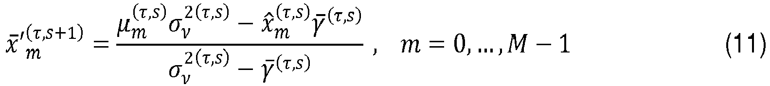

![]()
![]()
![]()
avec ε ≥ 0 étant une constante permettant de s'écarter de l'instabilité numérique. Des valeurs de l'ordre de ε = 10-3 ou 10-4 permettent d'améliorer les performances, sur les rares occurrences de blocs reçus où ![]()
D'autres stratégies sont possibles dans ce cas particulier ![]()
Par exemple, le bloc 306 peut fournir en sortie l'information a priori en provenance du décodeur, calculé à l'initialisation du démodulateur souple SISO (non représenté sur la
Ces estimations extrinsèques sont passées au bloc de lissage adaptatif 307 dont la finalité est de lisser les estimations en entrée en prenant en compte les valeurs passées. Un algorithme possible implémenté par ce bloc est d'accumuler linéairement les estimations présentes et passées (auto-itération précédente) selon les formules suivantes qui peuvent être interprétées comme un filtrage : ![]()
![]()
![]()
![]()
![]()
![]()
![]()
Au final, selon l'une des méthodes décrites précédemment ou évidentes pour l'homme de l'art, le bloc de lissage adaptatif 307 génère des estimations extrinsèques lissées ![]()
![]()
![]()
![]()
![]()
![]()
![]()
The posterior probability
The non-normalized posterior ![]()
![]()
![]()
![]()
![]()
In the case where the prior probabilities at the input of the posterior probability ![]()
![]()
![]()
![]()
![]()
![]()
![]()
In the case of a priori non-constant probabilities, the new estimation of the emitted symbols, generated by combining the a priori information available with the information contained in the observation according to the invention has characteristics superior to the estimate a priori. , or an estimate derived from the single observation. Within the framework of the theory of "expectation propagation" (EP), this operation also makes it possible to project a mixed probabilistic description on the sent symbols (Gaussian variables for the observations, combined with a priori estimates which are categorical variables) on a single probabilistic description, according to a Gaussian model as described in reference [3]. In more detail, we use here a result of information theory, known as "reverse I-projection," or "M-projection," which states that finding an exponential-type distribution ( in our case, Gaussian) which minimizes the divergence of Kullback-Leibler (a measure of probabilistic distance) with respect to any distribution, amounts to finding the exponential distribution having the same statistical moments ("moment matching").
The posterior variances are then averaged by the ![]()
Post hoc estimates ![]()
![]()
![]()
![]()
![]()
![]()
![]()
![]()
with ε ≥ 0 being a constant allowing to deviate from the numerical instability. Values of the order of ε = 10 -3 or 10 -4 allow to improve the performances, on the rare occurrences of blocks received where ![]()
Other strategies are possible in this particular ![]()
For example, the
These extrinsic estimates are passed to the ![]()
![]()
![]()
![]()
![]()
![]()
![]()
In the end, according to one of the methods previously described or obvious to those skilled in the art, the ![]()
![]()
Nous décrivons maintenant le fonctionnement du démodulateur souple SISO 105 quand ![]()
![]()
![]()
Par un procédé appelé dans la littérature « marginalisation » [4], les ![]()
![]()

![]()
Dans des implémentations sur des programmes d'ordinateur ou sur du matériel ,il convient aussi de maitriser la dynamique des LLRs du demapping souple et du décodeur afin de stabiliser, rendre plus robuste le comportement de l'algorithme, et de réduire son occupation mémoire tout en gardant des performances acceptables. Différentes stratégies telles que décrites dans les références [5], [6], [7] sont possibles et peuvent être appliquées indépendamment du procédé décrit ci-dessus.We now describe the operation of the ![]()
![]()
![]()
By a process called in the literature "marginalization" [4], the ![]()
![]()
![]()
In implementations on computer programs or on hardware, it is also necessary to master the dynamics of the LLRs of the flexible demapping and the decoder in order to stabilize, make more robust the behavior of the algorithm, and to reduce its memory occupation while keeping acceptable performance. Different strategies as described in references [5], [6], [7] are possible and can be applied independently of the method described above.
Les ![]()
![]()
![]()
![]()
![]()
![]()
![]()
![]()
![]()
![]()
Dans les mêmes hypothèses, la ![]()
![]()
Sans sortir du cadre de l'invention, le procédé peut s'appliquer dans différentes structures d'égaliseur, dont quelques exemples sont donnés ci-après à titre illustratif et nullement limitatif.Without departing from the scope of the invention, the method can be applied in different equalizer structures, some examples of which are given below by way of illustration and in no way limitative.
L'invention peut s'appliquer à un égaliseur turbo fractionnaire voir par exemple [8]. Dans ce contexte, l'unique différence est que le signal en provenance de l'antenne est sur-échantillonné avec un facteur avec un facteur o > 1, typiquement entier. En faisant référence à la
L'invention peut s'appliquer à un égaliseur de type Overlap FDE [9]. Dans ce type de récepteur, le bloc de données entre deux séquences pilotes est plus long du bloc de traitement, et pour des questions de complexité ou de nécessité (par exemple un canal variable dans le temps qui change dans l'horizon d'un bloc de données), le traitement d'égalisation fréquentiel est décomposé sur plusieurs segments (avec recouvrement) du bloc de données initial. Ces segments souffrent d'une interférence entre eux. Cela implique que la matrice de covariance du bruit en sortie du bloc d' « estimation de canal et de variance du bruit » 104 inclut aussi la variance due à l'interférence, ce qui modifie les valeurs du filtre d'égalisation.The invention can be applied to an overlap equalizer FDE [9]. In this type of receiver, the data block between two pilot sequences is longer than the processing block, and for complexity or necessity issues (for example a time-varying channel that changes in the horizon of a block of data), the frequency equalization process is broken down into several segments (with overlapping) of the initial data block. These segments suffer from interference between them. This implies that the noise covariance matrix at the output of the "channel estimate and noise variance"
L'invention peut être appliquée à la fois dans des stratégies de réjection d'interférence [10] et de suppression d'interférence [11]. Dans ce dernier cas, la variance ![]()
![]()
La technique proposée peut s'appliquer aussi à des égaliseurs linéaires au sens large.The proposed technique can also be applied to linear equalizers in the broad sense.
De manière générale, l'invention peut être utilisée au sein de tout type de récepteur itératif étant structuré comme illustré sur la
En effet, on considère disposer d'un émetteur 10 utilisant une modulation 13, une mise en trame 14 et une chaîne RF 15, quelconques, sur un bloc de données x pour le transmettre à travers un canal de propagation quelconque. On considère disposer d'un frontal RF 500 qui extrait l'observation y du signal, reçu à l'antenne, perturbé par le canal de communication, et qui le fournit au bloc d'estimation canal 501. Cet estimateur extrait du signal y, les séquences pilotes, afin d'utiliser une des techniques d'estimations, connues de l'homme de l'art, pour obtenir des paramètres caractérisant le canal. On suppose disposer d'un bloc « récepteur adaptatif à suppression d'interférence » 502, capable de fournir une estimation x̂ = x + v modélisée selon un modèle statistique gaussien additif ( v étant le bruit gaussien équivalent ajouté au signal utile). L'estimation x̂ est obtenue grâce à un procédé de suppression d'interférence qui, en utilisant une estimation préalable
Par ailleurs, on dispose d'un bloc de calcul des paramètres du récepteur 503, qui utilise les estimations du canal et la fiabilité de l'estimation préalable ![]()
![]()
L'invention s'applique au niveau du démodulateur souple 504, où, pour un bloc de données avec des statistiques supposées blanches, la technique de propagation d'espérance est utilisée pour calculer les estimations souples ![]()
![]()
Si les bits transmis ont été traités au préalable par un encodeur canal (comme par exemple dans l'émetteur 10 détaillé à la
En effet, l'invention porte, notamment, sur la technique de l'estimation du signal transmis, au niveau du démodulateur souple 504 qui travaille sur un modèle équivalent à un bruit additif gaussien. Elle peut être utilisée au sein de tout récepteur itératif qui passe par une telle étape de démodulation et se distingue des démodulateurs durs, utilisés entre autres dans les égaliseurs à retour de décision conventionnels, qui sont sujets à des problèmes de propagation de l'erreur. La technique considérée ici est différente aussi des techniques de démodulation souple utilisant une estimation a posteriori du signal, qui n'enlèvent pas de l'estimation du signal de retour l'information déjà connue par le récepteur, induisant ainsi le récepteur à l'erreur en le biaisant avec ses propres informations. Comparée à d'autres techniques d'estimation avec propagation d'espérance utilisées dans les récepteurs, le procédé selon l'invention fournit une fiabilité moyenne par bloc de données, ce qui permet de rendre le récepteur moins complexe et plus robuste face à des erreurs ponctuelles d'estimation. Par ailleurs, l'invention applique un lissage adaptatif sur le signal estimé, afin de fournir un degré de liberté additionnel qui permet de calibrer le rapport entre la robustesse des performances et la vitesse de convergence du récepteur vers les performances limites.Indeed, the invention relates, in particular, to the technique of estimating the transmitted signal, at the level of the
Par simplicité, les cas d'utilisations décrits ci-dessus, s'intéressent au traitement d'un signal mono-antennaire provenant d'un seul utilisateur. Nous allons montrer par un exemple d'usage que l'invention peut être utilisée au sein d'un récepteur multiutilisateur itératif.For simplicity, the use cases described above, are interested in the processing of a single-antennal signal from a single user. We will show by an example of use that the invention can be used within an iterative multi-user receiver.
L'invention s'applique aussi au cas mono-utilisateur single input multiple output (SIMO), c'est-à-dire à un système de communications avec un seul émetteur et un seul récepteur utilisant R antennes à la réception.The invention also applies to the single-user single-input multiple output (SIMO) case, that is to say to a communications system with a single transmitter and a single receiver using R antennas at reception.
L'invention s'applique aussi au cas mono-utilisateur multiple input multiple output (MIMO) où le seul émetteur est doté de plusieurs, Tu , antennes de transmission.The invention also applies to the multiple input multiple-output (MIMO) multiple-user case where the single transmitter is provided with several, T u , transmission antennas.
L'invention s'applique aussi à un système de transmission sans fil multi-utilisateurs, où les utilisateurs u(101,..10 u ) sont dotés d'une antenne (Tu = 1) et le récepteur 20 est doté de R antennes où R peut être égal à un ou plus. Nous supposons que U utilisateurs transmettent vers le récepteur et utilisent les mêmes ressources temporelles et fréquentielles. Le système est représenté en
L'invention s'applique aussi à un système de transmission sans fil multiutilisateur, où les utilisateurs u(101,..10 u ) sont dotés d'une ou plusieurs antennes (Tu ≥ 1) et le récepteur 20 est doté de R antennes ou R ≥ 1. Nous supposons que U utilisateurs transmettent vers le récepteur et utilisent les mêmes ressources temporelles et fréquentielles. Le système est représenté en
Nous décrivons l'invention d'abord dans le cas simple d'un récepteur multi-antennaire dans le cadre d'un système de type MU-MIMO. Nous notons que les autres scénarios ne sont que des cas particuliers de ce dernier et peuvent s'en déduire. Par exemple le cas MIMO avec un seul émetteur, s'obtient avec U = 1, l'émetteur est donc doté de T 1 antennes d'émission et le récepteur de R antennes de réception. Nous notons que lorsque T 1 = 1, R > 1, nous obtenons un système SIMO mono utilisateur. Lorsque U > 1, Tu = 1, R > 1, le système MU-MIMO peut être vu aussi comme un système SIMO multi-utilisateur. Lorsque U > 1 et R = 1, nous sommes en présence d'un système MU-MISO.We describe the invention first in the simple case of a multi-antennal receiver in the context of a MU-MIMO type system. We note that the other scenarios are only special cases of the latter and can be deduced from them. For example the case MIMO with a single transmitter, is obtained with U = 1, the transmitter is equipped with T 1 transmit antennas and the receiver of R receiving antennas. We note that when T 1 = 1, R > 1, we obtain a SIMO single-user system. When U > 1, T u = 1, R > 1, the MU-MIMO system can also be seen as a multi-user SIMO system. When U > 1 and R = 1, we are in the presence of a MU-MISO system.
La ![]()
![]()
Le code correcteur, l'entrelaceur, le modulateur et la génération de séquences pilotes peuvent présenter des caractéristiques différentes choisies en fonction de l'utilisateur. De plus, le modulateur peut présenter des caractéristiques différentes choisies en fonction de l'antenne d'émission pour un utilisateur donné.The correction code, the interleaver, the modulator and the generation of pilot sequences may have different characteristics chosen according to the user. In addition, the modulator may have different characteristics chosen according to the transmitting antenna for a given user.
La
Comme pour le cas SISO (![]()
![]()
![]()
![]()
![]()
![]()
![]()
![]()
Comme pour le cas SISO, dans la suite, les paramètres en entrée ou en sortie des blocs 106, 108, 105T, à l'exception des observations initiales y 1,...,y R sur les différentes antennes, et des estimations initiales H , Σ w , dépendent de l'identifiant de la turbo-itération courante
![]()
![]()
![]()
![]()
![]()
![]()
![]()
![]()
![]()
![]()
![]()
![]()
![]()
![]()
![]()
![]()
Les quantités échangées par le récepteur itératif de la ![]()
![]()
Comme dans le cas SISO, il convient d'initialiser les blocs au début du traitement de réception et au début de chaque turbo-itération, donc pour chaque
![]()
![]()
La description qui suit est donnée pour un cas SC-FDMA. Après avoir extrait les blocs de données en provenance des antennes du récepteur (à travers la suppression du CP dans le cas des systèmes SC avec CP ou du SC-FDMA, 101), les blocs sont soumis à une transformation de Fourier rapide 102 (Fast Fourier Transform - FFT) de taille N (passage dans le domaine fréquentiel). Ensuite, les signaux en sortie des FFTs passent dans des blocs « De-alloc sous-p » 103 qui sélectionnent uniquement les éléments des vecteurs correspondants aux sous-porteuses où les signaux ont été envoyés (dé-allocation des sous-porteuses). En sortie de ces derniers blocs, les signaux sont représentés par R vecteurs y r de taille M. Pour faciliter et simplifier la lecture du document par la suite, ces vecteurs peuvent être concaténés l'un à la suite de l'autre dans un vecteur y de taille MR. The following description is given for an SC-FDMA case. After extracting the data blocks from the receiver's antennas (by removing the CP in the case of SC systems with CP or SC-FDMA, 101), the blocks are subjected to Fast Fourier Transform (FFT) of size N (frequency domain transition). Then, the output signals of the FFTs pass into "sub-p-alloc" blocks 103 which select only the elements of the vectors corresponding to the sub-carriers where the signals have been sent (sub-carrier de-allocation). At the output of these last blocks, the signals are represented by R vectors y r of size M. To facilitate and simplify the reading of the document later, these vectors can be concatenated one after the other in a vector y of size MR.
En parallèle, les séquences pilotes sont extraites des signaux en provenance de l'antenne de réception et envoyées dans le bloc « Estimation des canaux et de la variance du bruit » 104 et utilisées pour calculer une estimation de la réponse fréquentielle des canaux MIMO entre les émetteurs et le récepteur, sur les M sous-porteuses d'intérêts (celles utilisées par les utilisateurs pour envoyer l'information). La réponse fréquentielle du canal entre l'antenne t de l'utilisateur u et l'antenne r du récepteur est organisée dans un vecteur h r,t,u de taille M, ou de façon équivalente, dans une matrice diagonale H r,t,u = diag( h r,t,u ) de taille M x M. Pour faciliter la lisibilité du document, les matrices correspondantes à une antenne de transmission t d'un utilisateur u peuvent être concaténées dans une matrice bloc-diagonale H t,u de taille MR x M. Ces dernières peuvent être concaténées séquentiellement dans une matrice bloc-diagonale H de taille MR x MT, les canaux des antennes des émetteurs sont concaténés sur la même ligne, pour la même antenne de réception. La quantité ![]()
![]()
Une fois que les observations et les estimations du canal MU-MIMO global H et de la covariance du bruit sont disponibles, la première boucle de traitement (auto-itération) est activée. Au tout premier passage (τ = 0), ou à chaque début de turbo-itération
![]()
- a) vide ses registres internes ;
- b) met à zéro les entrées des U vecteurs (signaux égalisés) x̂ u de longueur TuM formés par la concaténation des vecteurs x̂ t,u de taille M (signal égalisé de l'antenne t de l'utilisateur u) ;
- c) pose les entrées des vecteurs
- d) à la toute première activation de la phase d'initialisation (τ = 0) les informations a priori en provenance des
blocs 112u sont mises par convention égales à des vecteurs de zéros ; - e) les
blocs 105Tu de lafigure 13 s'exécutent avec un indice d'auto-itération s = -1, notamment en utilisant d'éventuelles entrées non-nulles d'information a priori en provenance des décodeurs 111u et plus précisément des blocs 112u (pour tous les u = 1, ..., U). La notation Tu est une convention indiquant à la fois que c'est le démodulateur de l'utilisateur u (en indice) et que l'entrée est égale aux signaux égalisés des Tu antennes de l'utilisateur u. Ainsi, pour tout u,le bloc 105Tu génère une estimation souplex u de longueur TuM formée par la concaténation des vecteursx t,u de taille M (estimation souple du signal de l'antenne t de l'utilisateur u) et le vecteur de leurs fiabilités correspondantesv u = [v 1, u, ...,vt ,u , ...,v Tu ,u], qui collecte une fiabilité par antenne de l'utilisateur u.
Nous notons qu'à la toute première activation de la phase d'initialisation (τ = 0) les estimations souplesx u seront des vecteurs nuls et

- f) Les sorties vers les
blocs 110u, désentrelaceurs, ne sont pas calculées parce qu'inutiles.
- a) empty its internal registers;
- b) resets the inputs of the U vectors (equalized signals) x u of length T u M formed by the concatenation of the vectors x t, u of size M (equalized signal of the antenna t of the user u ) ;
- c) poses vector inputs
- d) at the very first activation of the initialization phase ( τ = 0) the prior information from the
blocks 112 u is conventionally equal to zero vectors; - e) the
blocks 105T u of thefigure 13 execute with an index of self-iteration s = -1, in particular by using any non-zero inputs of a priori information fromdecoders 111 u and more precisely blocks 112 u (for all u = 1, ..., U ). The notation T u is a convention indicating both that it is the demodulator of the user u (in subscript) and that the input is equal to the equalized signals of the T u antennas of the user u. Thus, for all u, theblock 105T u generates a flexible estimatex u of length T u M formed by the concatenation of vectorsx t, u of size M (flexible estimate of the signal of the antenna t of the user u ) and the vector of their corresponding reliabilitiesv u = [v 1, u , ...,v t , u , ...,v Tu , u ], which collects an antenna reliability of the user u.
We note that at the very first activation of the initialization phase ( τ = 0) the soft estimatesx u will be zero vectors and - f) The outputs to the
blocks 110 u , deinterleavers, are not calculated because they are useless.
Pendant une turbo-itération donnée, quand les paquets de l'ensemble des utilisateurs ui ont été décodés, en ayant ainsi généré des informations souples, plusieurs stratégies d'initialisation sont possibles. La première est que le bloc « Gestionnaire d'ordonnancement et d'initialisation »
L'estimation du canal global MU-MIMO H et de la matrice de covariance du bruit sont passées au bloc « calcul des paramètres de l'égaliseur» 106. Ce bloc prend aussi en entrée les ![]()
![]()
![]()
![]()
![]()
![]()
![]()
![]()
Le bloc de calcul des paramètres de l'égaliseur fournit aussi en sortie les vecteurs ![]()
![]()


![]()
![]()
![]()
![]()
Les vecteurs de signaux reçus sur des antennes et transformés en fréquence y r de taille M sont passés au bloc « égaliseur linéaire à suppression d'interférence » 108 qui reçoit aussi en entrée les coefficients des égaliseurs F u , pour tous les utilisateurs u (qui sont traités parallèlement), la réponse fréquentielle globale du canal MU-MIMO H et les vecteurs de taille M d'estimations souples des symboles émis dans le domaine fréquentiel
Les vecteurs x̂ t,u sont ensuite passés à nouveau dans le domaine temporel à travers Tu IFFT normalisées de taille M (109), pour obtenir des vecteurs x̂ t,u représentant les signaux temporels égalisés, qui sont envoyés au démodulateur souple MU-MIMO 105T. Ce dernier, à partir des x̂ t,u , des correspondantes variances du bruit après égalisation ![]()
![]()
A ce moment, si l'ordonnancement commande d'exécuter une boucle d'auto-itération, les traitements poursuivent avec une réactivation des blocs 107, 106, 108, 109, 105T.At this time, if the scheduling command to execute an auto-iteration loop, the processes continue with a reactivation of the
Autrement, si l'ordonnancement commande d'exécuter une nouvelle boucle d'auto-itération ou de continuer la boucle de turbo-itération courante, les métriques souples Le ( du ), u ∈ u i sont ensuite désentrelacées par les blocs 110u pour les utilisateurs u ∈ u i. Ensuite, les métriques souples sont envoyées aux décodeurs 111u des utilisateurs u ∈ u i qui produisent des estimations des probabilités des bits d'informations envoyés (par exemple des probabilités a posteriori), si la dernière turbo-itération est atteinte, i.e.
![]()
![]()
Le démodulateur souple MU-MIMO 105T traite ses entrées et la procédure continue en fonction de l'activation d'une auto-itération ou d'une turbo-itération.The MU-
Le bloc «égaliseur linéaire à suppression d'interférence » 108 réalise la suppression d'interférence (IC) pour l'ISI, le MAI et le MUI et égalise les signaux reçus dans le domaine fréquentiel et spatial. Comme pour le cas SISO, la différence par rapport à l'état de l'art existant réside dans les entrées
La
Nous détaillons par la suite la structure du démodulateur souple MU-MIMO 105T. Comme il a été écrit pour la phase d'initialisation, le démodulateur souple MU-MIMO 105T représenté en ![]()
![]()
![]()
![]()
![]()
![]()
![]()
![]()
![]()
![]()
![]()
![]()
Nous allons détailler le bloc de démodulateur souple MIMO 105Tu, qui s'applique à un émetteur MIMO comme celui illustré à la ![]()
![]()
![]()
![]()
Dans le cas particulier d'un système mono-utilisateur (MIMO, autrement dit le cas où U = 1 avec T 1 antennes d'émission, un seul bloc de démodulateur souple MIMO 105Tu est utilisé au récepteur MIMO, et les symboles émis sont dénotés x t,1 , avec le mot de code correspondant d 1.In the particular case of a single-user system (MIMO, in other words the case where U = 1 with T 1 transmit antennas, a
L'invention s'applique aussi trivialement pour l'homme de l'art aux schémas avec des codes espace-temps par blocs de type orthogonal, comme celui d'Alamouti et décrit pour le cas SC-FDMA dans l'article [12], par exemple. Ces schémas ne sont pas représentés. Dans le cas des codes espace-temps par blocs de type orthogonal, il existe des méthodes de détection connues de l'homme de l'art [12] à maximum de vraisemblance ou à maximum de probabilité a posteriori avec complexité réduite. L'invention décrite ici peut s'appliquer après avoir adapté les calculs du bloc d'égalisation linéaire à suppression d'interférence 502 et le bloc de calcul des paramètres du récepteur 503, par exemple comme décrit dans [12] de façon à prendre en compte la structure du code espace-temps par blocs de type orthogonal utilisé à l'émetteur.The invention is also applied trivially to those skilled in the art in schemes with orthogonal block-type space-time codes, such as that of Alamouti and described for SC-FDMA in article [12] , for example. These diagrams are not represented. In the case of orthogonal block-type space-time codes, there are detection methods known to those skilled in the art [12] with maximum likelihood or with a posterior probability maximum with reduced complexity. The invention described here can be applied after having adapted the calculations of the interference canceling
-
[1]
P. Chevalier, F. Pipon, "New Insigths into Optimal Widely Linear Array Receivers for the Demodulation of BPSK, MSK, and GMSK Signais corrupted by Noncircular Interferences - Application to SAIC", IEEE Trans. on Signal Processing, v. 54, n. 3, pp: 870-883, March 2006 P. Chevalier, F. Pipon, "New Insigths into Optimal Widely Linear Array Receivers for the Demodulation of BPSK, MSK, and GMSK Signals corrupted by Noncircular Interferences - Application to SAIC", IEEE Trans. on Signal Processing, v. 54, n. 3, pp: 870-883, March 2006 -
[2]
M. Tüchler, A. C. Singer, "Turbo Equalization: An Overview," IEEE Trans. Information Theory, vol. 57, no. 2, pp. 920-952, fevrier 2011 Mr. Tüchler, AC Singer, "Turbo Equalization: An Overview," IEEE Trans. Information Theory, vol. 57, no. 2, pp. 920-952, February 2011 -
[3]
Thomas Minka, « Divergence measures and message passing », Microsoft Research, MSR-TR-2005-173, décembre 2005 Thomas Minka, "Divergence Measurements and Message Passing", Microsoft Research, MSR-TR-2005-173, December 2005 -
[4]
S. ten Brink, J. Speidel, R.-H. Yan, "Iterative Demapping and Decoding for Multilevel Modulation", IEEE GLOBECOM 1998 S. ten Brink, J. Speidel, R.-H. Yan, "Iterative Demapping and Decoding for Multilevel Modulation", IEEE GLOBECOM 1998 -
[5]
Q. Wang, Q. Xie, Z. Wang, S. Chen, L. Hanzo, "A Universal Low-Complexity Symbol-to-Bit Soft Demapper", IEEE Trans. On Vehicular Technology, 2014 Q. Wang, Q. Xie, Z. Wang, S. Chen, L. Hanzo, "A Universal Low-Complexity Symbol-to-Bit Soft Demapper", IEEE Trans. On Vehicular Technology, 2014 -
[6]
D. Auras, R. Leupers, G. Ascheid, "A Novel Class of Linear MIMO Detectors with Boosted Communications Performance: Algorithm and VLSI Architecture", IEEE ISVLSI 2014 D. Auras, R. Leupers, G. Ascheid, "A Novel Class of Linear MIMO Detectors with Boosted Communications Performance: Algorithm and VLSI Architecture," IEEE ISVLSI 2014 -
[7]
I. Collings, M. Butler and M. McKay, "Low Complexity receiver design for MIMO bit-interleaved coded modulation", IEEE ISSSTA 2004 I. Collings, M. Butler and M. McKay, "Low Complexity receiver design for MIMO bit-interleaved coded modulation", IEEE ISSSTA 2004 -
[8]
N. Benvenuto, S. Ciccotosto, and S. Tomasin, "Iterative Block Fractionally Spaced Nonlinear Equalization for Wideband Channels", IEEE Wireless Communications Letters, vol. 4, no. 5, pp. 489-492, October 2015 N. Benvenuto, S. Ciccotosto, and S. Tomasin, "Iterative Block Fractionally Spaced Nonlinear Equalization for Wideband Channels," IEEE Wireless Communications Letters, Vol. 4, no. 5, pp. 489-492, October 2015 -
[9]
L. Martoyo, T. Weiss, F. Capar, F.K. Jondral, "Low Complexity CDMA Downlink Receiver based on Frequency Domain Equalization", IEEE VTC'03 Fall, 2003 L. Martoyo, T. Weiss, F. Capar, FK Jondral, "Low Complexity CDMA Downlink Receiver based on Frequency Domain Equalization", IEEE VTC'03 Fall, 2003 -
[10]
T. Obara, F. Adachi, "MMSE Weight for Single Carrier Overlap FDE", Proc. IEEE Asia Pacific Conférence on Communications, 2011 T. Obara, F. Adachi, "MMSE Weight for Single Carrier Overlap FDE", Proc. IEEE Asia Pacific Conference on Communications, 2011 -
[11]
S. Tomasin, "Overlap and save frequency domain DFE for throughput efficient single carrier transmission", IEEE PIMRC 2005 S. Tomasin, "Overlap and save frequency domain DFE for efficient carrier single carrier transmission", IEEE PIMRC 2005 -
[12]
S.-R. Lee, F.-B. Ueng, H.-F. Wang, and Y.-K. Chang, "Iterative multiuser détection for LDPC MIMO SC-FDMA communication systems", Wiley Trans Emerging Tel Tech. doi: 10.1002/ett.2773, 15 janvier 2014 S.-R. Lee, F.-B. Ueng, H.-F. Wang, and Y.-K. Chang, "Iterative Multiuser Detection for LDPC MIMO SC-FDMA Communication Systems", Wiley Trans Emerging Tel Tech. doi: 10.1002 / ett.2773, January 15th, 2014 -
[13]
N. Benvenuto, S. Tomasin, « Iterative Design and Détection of a DFE in the Frequency Domain », IEEE Trans. on Commun., v. 53, n. 11, pp: 1867-1875, Nov. 2005 N. Benvenuto, S. Tomasin, "Iterative Design and Detection of a DFE in the Frequency Domain", IEEE Trans. on Commun., v. 53, n. 11, pp: 1867-1875, Nov. 2005 -
[14]
M. Witzke, S. Bäro, F. Schreckenbach, and J. Hagenauer, "Iterative détection of MIMO signais with linear detectors," in Proc. Asilomar Conférence on Signais, Systems and Computers (ACSSC), Pacific Grove, CA, USA. IEEE, Nov. 2002 M. Witzke, S. Bäro, F. Schreckenbach, and J. Hagenauer, "Iterative Detection of MIMO Signed with Linear Detectors," in Proc. Asilomar Conference on Signs, Systems and Computers (ACSSC), Pacific Grove, CA, USA. IEEE, Nov. 2002 -
[15]
I. Santos, J. J. Murillo-Fuentes, R. Boloix-Tortosa, E. A. de Reyna, and P. M. Olmos, "Expectation propagation as turbo equalizer in ISI channels," IEEE Trans. Commun., vol. 65, no. 1, pp. 360-370, Jan. 2017 I. Santos, JJ Murillo-Fuentes, R. Boloix-Tortosa, EA of Reyna, and PM Olmos, "Expectation Spread As Turbo Equalizer in ISI Channels," IEEE Trans. Commun., Vol. 65, no. 1, pp. 360-370, Jan. 2017 -
[16]
K. Wu, G. Ren, X. Meng, J. Wu, Q. Wang, "Spectral-Efficient Band Allocation Scheme for Frequency-Domain Pulse Shaping-Based SC-FDMA Systems", IEEE Transactions on Vehicular Technology, Vol.: 66, n: 9, pp: 8249 - 8262, Sept. 2017 K. Wu, G. Ren, X. Meng, J. Wu, Wang Q., "Spectral-Efficient Band Allocation Scheme for Frequency-Domain Pulse Shaping-Based SC-FDMA Systems", IEEE Transactions on Vehicular Technology, Vol .: 66, n: 9, pp: 8249 - 8262, Sept. 2017 -
[17]
I. Santos, J. J. Murillo-Fuentes, P. M. Olmos, "Block expectation propagation equalization for ISI channels", 23rd European signal processingconference (EUSIPCO 2015), pp 379-383, 31 août 2015 I. Santos, JJ Murillo-Fuentes, PM Olmos, "Block expectation propagation equalization for ISI channels", 23rd European Signal Processing Conference (EUSIPCO 2015), pp 379-383, August 31, 2015
Claims (23)

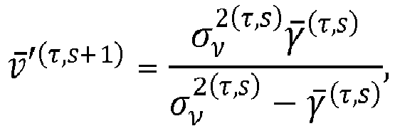
Un module de sélection (303) configuré pour sélectionner les estimés souples a priori
A selection module (303) configured to select soft estimates a priori
Priority Applications (1)
| Application Number | Priority Date | Filing Date | Title |
|---|---|---|---|
| PL19156763T PL3528443T3 (en) | 2018-02-15 | 2019-02-12 | Method for calculating an estimate of a modulated digital signal and its reliability |
Applications Claiming Priority (1)
| Application Number | Priority Date | Filing Date | Title |
|---|---|---|---|
| FR1800146A FR3077941A1 (en) | 2018-02-15 | 2018-02-15 | METHOD FOR CALCULATING AN ESTIMATION OF A MODULAR DIGITAL SIGNAL AND ITS RELIABILITY |
Publications (2)
| Publication Number | Publication Date |
|---|---|
| EP3528443A1 true EP3528443A1 (en) | 2019-08-21 |
| EP3528443B1 EP3528443B1 (en) | 2020-09-09 |
Family
ID=62167449
Family Applications (1)
| Application Number | Title | Priority Date | Filing Date |
|---|---|---|---|
| EP19156763.5A Active EP3528443B1 (en) | 2018-02-15 | 2019-02-12 | Method for calculating an estimate of a modulated digital signal and its reliability |
Country Status (4)
| Country | Link |
|---|---|
| EP (1) | EP3528443B1 (en) |
| ES (1) | ES2833540T3 (en) |
| FR (1) | FR3077941A1 (en) |
| PL (1) | PL3528443T3 (en) |
Cited By (6)
| Publication number | Priority date | Publication date | Assignee | Title |
|---|---|---|---|---|
| CN112104580A (en) * | 2020-09-11 | 2020-12-18 | 中海石油(中国)有限公司湛江分公司 | Sparse underwater acoustic channel estimation method based on generalized approximate message transfer-sparse Bayesian learning |
| FR3157997A1 (en) | 2023-12-28 | 2025-07-04 | Thales | Method for estimating a soft return signal in a turbo receiver based on expectation propagation |
| FR3157998A1 (en) | 2023-12-28 | 2025-07-04 | Thales | Method for calculating a correspondence table allowing the efficient implementation of a flexible modulator in a turbo receiver |
| FR3157999A1 (en) | 2023-12-28 | 2025-07-04 | Thales | Method for calculating a correspondence table between a variance of input samples of a flexible demodulator and a variance associated with LLR bits a priori in a turbo receiver |
| CN121367478A (en) * | 2025-12-22 | 2026-01-20 | 苏州大学 | Quantized perceptual wide-linearity minimum error mode adaptive filter |
| CN121508553A (en) * | 2026-01-14 | 2026-02-10 | 电子科技大学 | A Hadamard-LDPC Iterative Decoding Method Based on Interference Suppression |
Families Citing this family (1)
| Publication number | Priority date | Publication date | Assignee | Title |
|---|---|---|---|---|
| CN115167391B (en) * | 2022-06-14 | 2024-10-15 | 北京交通大学 | A virtual train formation control method based on sliding mode control |
-
2018
- 2018-02-15 FR FR1800146A patent/FR3077941A1/en not_active Withdrawn
-
2019
- 2019-02-12 ES ES19156763T patent/ES2833540T3/en active Active
- 2019-02-12 PL PL19156763T patent/PL3528443T3/en unknown
- 2019-02-12 EP EP19156763.5A patent/EP3528443B1/en active Active
Non-Patent Citations (2)
| Title |
|---|
| SANTOS IRENE ET AL: "Block expectation propagation equalization for ISI channels", 2015 23RD EUROPEAN SIGNAL PROCESSING CONFERENCE (EUSIPCO), EURASIP, 31 August 2015 (2015-08-31), pages 379 - 383, XP032836367, DOI: 10.1109/EUSIPCO.2015.7362409 * |
| WU KUN ET AL: "Spectral-Efficient Band Allocation Scheme for Frequency-Domain Pulse-Shaping-Based SC-FDMA Systems", IEEE TRANSACTIONS ON VEHICULAR TECHNOLOGY, IEEE SERVICE CENTER, PISCATAWAY, NJ, US, vol. 66, no. 9, 1 September 2017 (2017-09-01), pages 8249 - 8262, XP011660834, ISSN: 0018-9545, [retrieved on 20170919], DOI: 10.1109/TVT.2017.2683802 * |
Cited By (6)
| Publication number | Priority date | Publication date | Assignee | Title |
|---|---|---|---|---|
| CN112104580A (en) * | 2020-09-11 | 2020-12-18 | 中海石油(中国)有限公司湛江分公司 | Sparse underwater acoustic channel estimation method based on generalized approximate message transfer-sparse Bayesian learning |
| FR3157997A1 (en) | 2023-12-28 | 2025-07-04 | Thales | Method for estimating a soft return signal in a turbo receiver based on expectation propagation |
| FR3157998A1 (en) | 2023-12-28 | 2025-07-04 | Thales | Method for calculating a correspondence table allowing the efficient implementation of a flexible modulator in a turbo receiver |
| FR3157999A1 (en) | 2023-12-28 | 2025-07-04 | Thales | Method for calculating a correspondence table between a variance of input samples of a flexible demodulator and a variance associated with LLR bits a priori in a turbo receiver |
| CN121367478A (en) * | 2025-12-22 | 2026-01-20 | 苏州大学 | Quantized perceptual wide-linearity minimum error mode adaptive filter |
| CN121508553A (en) * | 2026-01-14 | 2026-02-10 | 电子科技大学 | A Hadamard-LDPC Iterative Decoding Method Based on Interference Suppression |
Also Published As
| Publication number | Publication date |
|---|---|
| PL3528443T3 (en) | 2021-03-08 |
| FR3077941A1 (en) | 2019-08-16 |
| EP3528443B1 (en) | 2020-09-09 |
| ES2833540T3 (en) | 2021-06-15 |
Similar Documents
| Publication | Publication Date | Title |
|---|---|---|
| EP3528443B1 (en) | Method for calculating an estimate of a modulated digital signal and its reliability | |
| EP2947799B1 (en) | Method of widely linear turbo-equalisation in a multi-user system and for a multi-antenna receiver | |
| EP1658694B1 (en) | Iterative decoding and equalizion method and apparatus for communication with multiple transmission and reception antennas | |
| EP2220803B1 (en) | Reduction of interference in an ofdm signal with weighting vectors evolving in vector subspaces | |
| EP3800813B1 (en) | Method and device for predicting the performance of a receiver in a communication system | |
| EP2274852A2 (en) | Method of decoding a signal implementing a progressive construction of a decoding tree, corresponding computer program product and decoding device | |
| EP1589685B1 (en) | Iterative chip equalization and multiuser detection for CDMA communications systems on MIMO channels | |
| FR2893433A1 (en) | METHODS AND DEVICES FOR FLEXIBLE DEMODULATION IN AN OFDM-CDMA SYSTEM | |
| EP1603264B1 (en) | Method and system for receiving a linearly precoded and channel coded signal | |
| EP1589672B1 (en) | Iterative vectorized equalization method for CDMA communications systems on MIMO channel | |
| EP1661286A1 (en) | Receiver and method for decoding a coded signal with the aid of a space-time coding matrix | |
| WO2006094860A1 (en) | Method for the iterative reception of a multicarrier signal with interference cancellation, and corresponding receiver and computer program | |
| EP1589673B1 (en) | Iterative multiuser detection method for CDMA communications systems on MIMO canal | |
| EP1999918B1 (en) | Method and device for receiving a data signal consisting of symbol blocks and corresponding computer program | |
| WO2002019557A1 (en) | Method and device for demodulating signals from multiusers | |
| FR2849306A1 (en) | Digital word packet radio propagation compensation having iterative feedback estimator/symbol detector with operations providing distinct channel estimates/removing word groups received dependent transmission conditions | |
| Petitpied | Faster-Than-Nyquist communication systems: from single-carrier to multi-carrier signaling | |
| WO2023213962A1 (en) | Continuous phase modulation receiver | |
| WO2016020611A1 (en) | Method and device for receiving signals | |
| CA2389592A1 (en) | Method and device for sequencing signals from multiusers | |
| Dietl | System Model for Iterative Multiuser Detection |
Legal Events
| Date | Code | Title | Description |
|---|---|---|---|
| PUAI | Public reference made under article 153(3) epc to a published international application that has entered the european phase |
Free format text: ORIGINAL CODE: 0009012 |
|
| STAA | Information on the status of an ep patent application or granted ep patent |
Free format text: STATUS: THE APPLICATION HAS BEEN PUBLISHED |
|
| AK | Designated contracting states |
Kind code of ref document: A1 Designated state(s): AL AT BE BG CH CY CZ DE DK EE ES FI FR GB GR HR HU IE IS IT LI LT LU LV MC MK MT NL NO PL PT RO RS SE SI SK SM TR |
|
| AX | Request for extension of the european patent |
Extension state: BA ME |
|
| STAA | Information on the status of an ep patent application or granted ep patent |
Free format text: STATUS: REQUEST FOR EXAMINATION WAS MADE |
|
| 17P | Request for examination filed |
Effective date: 20200217 |
|
| GRAP | Despatch of communication of intention to grant a patent |
Free format text: ORIGINAL CODE: EPIDOSNIGR1 |
|
| RBV | Designated contracting states (corrected) |
Designated state(s): AL AT BE BG CH CY CZ DE DK EE ES FI FR GB GR HR HU IE IS IT LI LT LU LV MC MK MT NL NO PL PT RO RS SE SI SK SM TR |
|
| STAA | Information on the status of an ep patent application or granted ep patent |
Free format text: STATUS: GRANT OF PATENT IS INTENDED |
|
| RIC1 | Information provided on ipc code assigned before grant |
Ipc: H04L 25/06 20060101ALI20200306BHEP Ipc: H04L 25/03 20060101AFI20200306BHEP |
|
| INTG | Intention to grant announced |
Effective date: 20200326 |
|
| GRAS | Grant fee paid |
Free format text: ORIGINAL CODE: EPIDOSNIGR3 |
|
| GRAA | (expected) grant |
Free format text: ORIGINAL CODE: 0009210 |
|
| STAA | Information on the status of an ep patent application or granted ep patent |
Free format text: STATUS: THE PATENT HAS BEEN GRANTED |
|
| AK | Designated contracting states |
Kind code of ref document: B1 Designated state(s): AL AT BE BG CH CY CZ DE DK EE ES FI FR GB GR HR HU IE IS IT LI LT LU LV MC MK MT NL NO PL PT RO RS SE SI SK SM TR |
|
| REG | Reference to a national code |
Ref country code: GB Ref legal event code: FG4D Free format text: NOT ENGLISH |
|
| REG | Reference to a national code |
Ref country code: AT Ref legal event code: REF Ref document number: 1312960 Country of ref document: AT Kind code of ref document: T Effective date: 20200915 Ref country code: CH Ref legal event code: EP |
|
| REG | Reference to a national code |
Ref country code: DE Ref legal event code: R096 Ref document number: 602019000579 Country of ref document: DE |
|
| REG | Reference to a national code |
Ref country code: IE Ref legal event code: FG4D Free format text: LANGUAGE OF EP DOCUMENT: FRENCH |
|
| REG | Reference to a national code |
Ref country code: FI Ref legal event code: FGE |
|
| REG | Reference to a national code |
Ref country code: LT Ref legal event code: MG4D |
|
| PG25 | Lapsed in a contracting state [announced via postgrant information from national office to epo] |
Ref country code: GR Free format text: LAPSE BECAUSE OF FAILURE TO SUBMIT A TRANSLATION OF THE DESCRIPTION OR TO PAY THE FEE WITHIN THE PRESCRIBED TIME-LIMIT Effective date: 20201210 Ref country code: LT Free format text: LAPSE BECAUSE OF FAILURE TO SUBMIT A TRANSLATION OF THE DESCRIPTION OR TO PAY THE FEE WITHIN THE PRESCRIBED TIME-LIMIT Effective date: 20200909 Ref country code: BG Free format text: LAPSE BECAUSE OF FAILURE TO SUBMIT A TRANSLATION OF THE DESCRIPTION OR TO PAY THE FEE WITHIN THE PRESCRIBED TIME-LIMIT Effective date: 20201209 Ref country code: NO Free format text: LAPSE BECAUSE OF FAILURE TO SUBMIT A TRANSLATION OF THE DESCRIPTION OR TO PAY THE FEE WITHIN THE PRESCRIBED TIME-LIMIT Effective date: 20201209 Ref country code: HR Free format text: LAPSE BECAUSE OF FAILURE TO SUBMIT A TRANSLATION OF THE DESCRIPTION OR TO PAY THE FEE WITHIN THE PRESCRIBED TIME-LIMIT Effective date: 20200909 Ref country code: SE Free format text: LAPSE BECAUSE OF FAILURE TO SUBMIT A TRANSLATION OF THE DESCRIPTION OR TO PAY THE FEE WITHIN THE PRESCRIBED TIME-LIMIT Effective date: 20200909 |
|
| REG | Reference to a national code |
Ref country code: AT Ref legal event code: MK05 Ref document number: 1312960 Country of ref document: AT Kind code of ref document: T Effective date: 20200909 |
|
| REG | Reference to a national code |
Ref country code: NL Ref legal event code: MP Effective date: 20200909 |
|
| PG25 | Lapsed in a contracting state [announced via postgrant information from national office to epo] |
Ref country code: LV Free format text: LAPSE BECAUSE OF FAILURE TO SUBMIT A TRANSLATION OF THE DESCRIPTION OR TO PAY THE FEE WITHIN THE PRESCRIBED TIME-LIMIT Effective date: 20200909 Ref country code: RS Free format text: LAPSE BECAUSE OF FAILURE TO SUBMIT A TRANSLATION OF THE DESCRIPTION OR TO PAY THE FEE WITHIN THE PRESCRIBED TIME-LIMIT Effective date: 20200909 |
|
| PG25 | Lapsed in a contracting state [announced via postgrant information from national office to epo] |
Ref country code: EE Free format text: LAPSE BECAUSE OF FAILURE TO SUBMIT A TRANSLATION OF THE DESCRIPTION OR TO PAY THE FEE WITHIN THE PRESCRIBED TIME-LIMIT Effective date: 20200909 Ref country code: PT Free format text: LAPSE BECAUSE OF FAILURE TO SUBMIT A TRANSLATION OF THE DESCRIPTION OR TO PAY THE FEE WITHIN THE PRESCRIBED TIME-LIMIT Effective date: 20210111 Ref country code: RO Free format text: LAPSE BECAUSE OF FAILURE TO SUBMIT A TRANSLATION OF THE DESCRIPTION OR TO PAY THE FEE WITHIN THE PRESCRIBED TIME-LIMIT Effective date: 20200909 Ref country code: CZ Free format text: LAPSE BECAUSE OF FAILURE TO SUBMIT A TRANSLATION OF THE DESCRIPTION OR TO PAY THE FEE WITHIN THE PRESCRIBED TIME-LIMIT Effective date: 20200909 Ref country code: SM Free format text: LAPSE BECAUSE OF FAILURE TO SUBMIT A TRANSLATION OF THE DESCRIPTION OR TO PAY THE FEE WITHIN THE PRESCRIBED TIME-LIMIT Effective date: 20200909 |
|
| PG25 | Lapsed in a contracting state [announced via postgrant information from national office to epo] |
Ref country code: AL Free format text: LAPSE BECAUSE OF FAILURE TO SUBMIT A TRANSLATION OF THE DESCRIPTION OR TO PAY THE FEE WITHIN THE PRESCRIBED TIME-LIMIT Effective date: 20200909 Ref country code: AT Free format text: LAPSE BECAUSE OF FAILURE TO SUBMIT A TRANSLATION OF THE DESCRIPTION OR TO PAY THE FEE WITHIN THE PRESCRIBED TIME-LIMIT Effective date: 20200909 Ref country code: IS Free format text: LAPSE BECAUSE OF FAILURE TO SUBMIT A TRANSLATION OF THE DESCRIPTION OR TO PAY THE FEE WITHIN THE PRESCRIBED TIME-LIMIT Effective date: 20210109 |
|
| REG | Reference to a national code |
Ref country code: DE Ref legal event code: R097 Ref document number: 602019000579 Country of ref document: DE |
|
| REG | Reference to a national code |
Ref country code: ES Ref legal event code: FG2A Ref document number: 2833540 Country of ref document: ES Kind code of ref document: T3 Effective date: 20210615 |
|
| PG25 | Lapsed in a contracting state [announced via postgrant information from national office to epo] |
Ref country code: SK Free format text: LAPSE BECAUSE OF FAILURE TO SUBMIT A TRANSLATION OF THE DESCRIPTION OR TO PAY THE FEE WITHIN THE PRESCRIBED TIME-LIMIT Effective date: 20200909 |
|
| PLBE | No opposition filed within time limit |
Free format text: ORIGINAL CODE: 0009261 |
|
| STAA | Information on the status of an ep patent application or granted ep patent |
Free format text: STATUS: NO OPPOSITION FILED WITHIN TIME LIMIT |
|
| 26N | No opposition filed |
Effective date: 20210610 |
|
| PG25 | Lapsed in a contracting state [announced via postgrant information from national office to epo] |
Ref country code: DK Free format text: LAPSE BECAUSE OF FAILURE TO SUBMIT A TRANSLATION OF THE DESCRIPTION OR TO PAY THE FEE WITHIN THE PRESCRIBED TIME-LIMIT Effective date: 20200909 Ref country code: SI Free format text: LAPSE BECAUSE OF FAILURE TO SUBMIT A TRANSLATION OF THE DESCRIPTION OR TO PAY THE FEE WITHIN THE PRESCRIBED TIME-LIMIT Effective date: 20200909 |
|
| PG25 | Lapsed in a contracting state [announced via postgrant information from national office to epo] |
Ref country code: MC Free format text: LAPSE BECAUSE OF FAILURE TO SUBMIT A TRANSLATION OF THE DESCRIPTION OR TO PAY THE FEE WITHIN THE PRESCRIBED TIME-LIMIT Effective date: 20200909 |
|
| REG | Reference to a national code |
Ref country code: BE Ref legal event code: MM Effective date: 20210228 |
|
| PG25 | Lapsed in a contracting state [announced via postgrant information from national office to epo] |
Ref country code: LU Free format text: LAPSE BECAUSE OF NON-PAYMENT OF DUE FEES Effective date: 20210212 |
|
| PG25 | Lapsed in a contracting state [announced via postgrant information from national office to epo] |
Ref country code: IE Free format text: LAPSE BECAUSE OF NON-PAYMENT OF DUE FEES Effective date: 20210212 |
|
| PG25 | Lapsed in a contracting state [announced via postgrant information from national office to epo] |
Ref country code: BE Free format text: LAPSE BECAUSE OF NON-PAYMENT OF DUE FEES Effective date: 20210228 |
|
| REG | Reference to a national code |
Ref country code: CH Ref legal event code: PL |
|
| PG25 | Lapsed in a contracting state [announced via postgrant information from national office to epo] |
Ref country code: LI Free format text: LAPSE BECAUSE OF NON-PAYMENT OF DUE FEES Effective date: 20220228 Ref country code: CH Free format text: LAPSE BECAUSE OF NON-PAYMENT OF DUE FEES Effective date: 20220228 |
|
| PG25 | Lapsed in a contracting state [announced via postgrant information from national office to epo] |
Ref country code: NL Free format text: LAPSE BECAUSE OF NON-PAYMENT OF DUE FEES Effective date: 20200923 Ref country code: CY Free format text: LAPSE BECAUSE OF FAILURE TO SUBMIT A TRANSLATION OF THE DESCRIPTION OR TO PAY THE FEE WITHIN THE PRESCRIBED TIME-LIMIT Effective date: 20200909 |
|
| PG25 | Lapsed in a contracting state [announced via postgrant information from national office to epo] |
Ref country code: HU Free format text: LAPSE BECAUSE OF FAILURE TO SUBMIT A TRANSLATION OF THE DESCRIPTION OR TO PAY THE FEE WITHIN THE PRESCRIBED TIME-LIMIT; INVALID AB INITIO Effective date: 20190212 |
|
| GBPC | Gb: european patent ceased through non-payment of renewal fee |
Effective date: 20230212 |
|
| PG25 | Lapsed in a contracting state [announced via postgrant information from national office to epo] |
Ref country code: GB Free format text: LAPSE BECAUSE OF NON-PAYMENT OF DUE FEES Effective date: 20230212 |
|
| PG25 | Lapsed in a contracting state [announced via postgrant information from national office to epo] |
Ref country code: GB Free format text: LAPSE BECAUSE OF NON-PAYMENT OF DUE FEES Effective date: 20230212 |
|
| PG25 | Lapsed in a contracting state [announced via postgrant information from national office to epo] |
Ref country code: MK Free format text: LAPSE BECAUSE OF FAILURE TO SUBMIT A TRANSLATION OF THE DESCRIPTION OR TO PAY THE FEE WITHIN THE PRESCRIBED TIME-LIMIT Effective date: 20200909 |
|
| PG25 | Lapsed in a contracting state [announced via postgrant information from national office to epo] |
Ref country code: MT Free format text: LAPSE BECAUSE OF FAILURE TO SUBMIT A TRANSLATION OF THE DESCRIPTION OR TO PAY THE FEE WITHIN THE PRESCRIBED TIME-LIMIT Effective date: 20200909 |
|
| PGFP | Annual fee paid to national office [announced via postgrant information from national office to epo] |
Ref country code: PL Payment date: 20250117 Year of fee payment: 7 |
|
| PG25 | Lapsed in a contracting state [announced via postgrant information from national office to epo] |
Ref country code: TR Free format text: LAPSE BECAUSE OF FAILURE TO SUBMIT A TRANSLATION OF THE DESCRIPTION OR TO PAY THE FEE WITHIN THE PRESCRIBED TIME-LIMIT Effective date: 20200909 |
|
| PGFP | Annual fee paid to national office [announced via postgrant information from national office to epo] |
Ref country code: ES Payment date: 20260311 Year of fee payment: 8 |
|
| PGFP | Annual fee paid to national office [announced via postgrant information from national office to epo] |
Ref country code: DE Payment date: 20260114 Year of fee payment: 8 |
|
| PGFP | Annual fee paid to national office [announced via postgrant information from national office to epo] |
Ref country code: FI Payment date: 20260213 Year of fee payment: 8 Ref country code: IT Payment date: 20260128 Year of fee payment: 8 |
|
| PGFP | Annual fee paid to national office [announced via postgrant information from national office to epo] |
Ref country code: FR Payment date: 20260121 Year of fee payment: 8 |