WO2020121943A1 - Système d'inspection, procédé d'inspection et programme - Google Patents
Système d'inspection, procédé d'inspection et programme Download PDFInfo
- Publication number
- WO2020121943A1 WO2020121943A1 PCT/JP2019/047673 JP2019047673W WO2020121943A1 WO 2020121943 A1 WO2020121943 A1 WO 2020121943A1 JP 2019047673 W JP2019047673 W JP 2019047673W WO 2020121943 A1 WO2020121943 A1 WO 2020121943A1
- Authority
- WO
- WIPO (PCT)
- Prior art keywords
- equation
- motion
- state
- variable
- angular displacement
- Prior art date
- Legal status (The legal status is an assumption and is not a legal conclusion. Google has not performed a legal analysis and makes no representation as to the accuracy of the status listed.)
- Ceased
Links
Images









Classifications
-
- B—PERFORMING OPERATIONS; TRANSPORTING
- B61—RAILWAYS
- B61L—GUIDING RAILWAY TRAFFIC; ENSURING THE SAFETY OF RAILWAY TRAFFIC
- B61L23/00—Control, warning or like safety means along the route or between vehicles or trains
- B61L23/04—Control, warning or like safety means along the route or between vehicles or trains for monitoring the mechanical state of the route
- B61L23/042—Track changes detection
- B61L23/047—Track or rail movements
-
- B—PERFORMING OPERATIONS; TRANSPORTING
- B61—RAILWAYS
- B61K—AUXILIARY EQUIPMENT SPECIALLY ADAPTED FOR RAILWAYS, NOT OTHERWISE PROVIDED FOR
- B61K9/00—Railway vehicle profile gauges; Detecting or indicating overheating of components; Apparatus on locomotives or cars to indicate bad track sections; General design of track recording vehicles
- B61K9/08—Measuring installations for surveying permanent way
Definitions
- the present invention relates to an inspection system, an inspection method, and a program, and is particularly suitable for being used for inspecting the track of a railway vehicle.
- the present application claims priority based on Japanese Patent Application No. 2018-230834 filed in Japan on December 10, 2018, the entire contents of which are incorporated herein.
- Patent Document 1 in the equation of motion describing the yaw of the wheel set, the angular displacement of the wheel set in the yawing direction, the state variable obtained by a filter that assimilates the data, and the front and rear directions generated in the member for supporting the axle box are described. There is disclosed a technique of substituting a measured value of a front-back direction force, which is a force in a direction, with a track irregularity (passage amount, etc.) of a railway vehicle.
- the present invention has been made in view of the above problems, and it is an object of the present invention to reduce the number of sensors used for detecting railroad track irregularities.
- the inspection system of the present invention is a data acquisition unit that acquires the data of the measured value of the front-rear direction force as the data of the measured value measured by running the railway vehicle having the vehicle body, the bogie, and the wheel axle on the track.
- a state variable deriving means for deriving a state variable which is a variable to be determined by a state equation constituted by using a motion equation describing the motion of the railway vehicle, by using the measured value of the longitudinal force
- the front-rear direction force is a front-rear direction force generated in a member arranged between the wheel shaft and the bogie on which the wheel shaft is provided.
- the front-rear direction is a direction along the traveling direction of the railway vehicle
- the yawing direction is a rotation direction having a vertical axis that is a direction perpendicular to the track as a rotation axis. Is an equation described using the state variable, the longitudinal force, and the conversion variable, and the state variable is the lateral displacement and velocity of the bogie and the yaw direction angle of the bogie.
- the rolling direction does not include the angular displacement and the angular velocity of the wheel axle in the yawing direction, and the rolling direction is a rotation direction with the front-rear direction as a rotation axis, and the conversion variable is the angular displacement of the wheel axle in the yawing direction and the trolley.
- a variable for mutually converting an angular displacement in the yawing direction wherein the track state deriving means is an angular displacement in the yawing direction of the carriage that is one of the state variables derived by the state variable deriving means, and
- the actual value of the conversion variable is used to derive an estimated value of the angular displacement of the wheel axle in the yawing direction, and the information that reflects the state of the track using the derived estimated value of the angular displacement of the wheel axle in the yawing direction.
- the actual value of the conversion variable is derived using the measured value of the front-back direction force, and the state variable deriving means, in the period in which the measured value of the front-back direction force is obtained, the trolley, the It is characterized in that the state variable is derived without using the measured values of the wheel axle and the lateral acceleration of the vehicle body.
- the inspection method of the present invention includes a data acquisition step of acquiring measurement value data of longitudinal force as measurement value data measured by running a railroad vehicle having a vehicle body, a bogie, and a wheel set on a track.
- the front-rear direction is a direction along the traveling direction of the railway vehicle
- the yawing direction is a rotation direction having a vertical axis that is a direction perpendicular to the track as a rotation axis. Is an equation described using the state variable, the longitudinal force, and the conversion variable, and the state variable is the lateral displacement and velocity of the bogie and the yaw direction angle of the bogie.
- the rolling direction does not include the angular displacement and the angular velocity of the wheel axle in the yawing direction, and the rolling direction is a rotation direction with the front-rear direction as a rotation axis, and the conversion variable is the angular displacement of the wheel axle in the yawing direction and the trolley.
- a variable for mutually converting the angular displacement in the yawing direction, and the trajectory state deriving step is an angular displacement in the yawing direction of the carriage that is one of the state variables derived by the state variable deriving step, and
- the actual value of the conversion variable is used to derive an estimated value of the angular displacement of the wheel axle in the yawing direction, and the information that reflects the state of the track using the derived estimated value of the angular displacement of the wheel axle in the yawing direction.
- the actual value of the conversion variable is derived using the measured value of the front-rear direction force, and the state variable derivation step, in the period in which the measured value of the front-rear direction force is obtained, It is characterized in that the state variable is derived without using the measured values of the wheel axle and the lateral acceleration of the vehicle body.
- the program of the present invention includes a data acquisition step of acquiring measurement value data of longitudinal force as measurement value data measured by running a railroad vehicle having a vehicle body, a bogie, and a wheel set on a track.
- a state variable deriving step of deriving a state variable which is a variable to be determined by a state equation formed by using a motion equation describing the motion of the railway vehicle, by using the measured value of the longitudinal force, and a state of the track.
- a track state deriving step of deriving information reflecting the information, and the front-rear direction force is a force in a front-rear direction generated in a member arranged between the wheel shaft and the carriage on which the wheel shaft is provided.
- the force is a force determined according to the difference between the angular displacement in the yawing direction of the wheel shaft and the angular displacement in the yawing direction of the carriage on which the wheel shaft is provided, and the member is a member for supporting the axle box.
- the front-back direction is a direction along the traveling direction of the railway vehicle
- the yawing direction is a rotation direction having a vertical axis that is a direction perpendicular to the track as a rotation axis.
- the equation is an equation described using the state variable, the longitudinal force, and the conversion variable, and the state variable is the lateral displacement and speed of the carriage and the yawing direction of the carriage.
- the rolling direction does not include the angular displacement and angular velocity of the wheel axle in the yawing direction, and the rolling direction is a rotational direction with the longitudinal axis as the rotational axis, and the conversion variable is the angular displacement of the wheel axle in the yawing direction and the carriage.
- the track state deriving step is an angular displacement in the yawing direction of the carriage that is one of the state variables derived by the state variable deriving step
- the actual value of the conversion variable is used to derive an estimated value of the angular displacement of the wheel axle in the yawing direction
- the derived estimated value of the angular displacement of the wheel axle in the yawing direction is used to reflect the state of the track.
- the actual value of the conversion variable is derived using the measured value of the longitudinal force, the state variable derivation step, in the period in which the measured value of the longitudinal force is obtained, the trolley, It is characterized in that the state variable is derived without using the measured values of the acceleration in the lateral direction of the vehicle body and the vehicle body.
- FIG. 1 is a diagram showing an example of an outline of a railway vehicle.
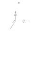
- FIG. 2 is a diagram conceptually showing the main directions of movement of the components of the railway vehicle.
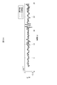
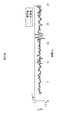
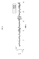
- FIG. 3 is a diagram showing a measured value and a calculated value in each of the lateral acceleration of the bogie and the lateral acceleration of the wheel axle.
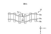
- FIG. 4A is a diagram showing an example of a deviation amount in a straight track.
- FIG. 4B is a diagram showing an example of a deviation amount in a curved track.
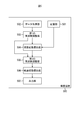
- FIG. 5 is a diagram illustrating an example of a functional configuration of the inspection device.
- FIG. 6 is a diagram illustrating an example of the hardware configuration of the inspection device.
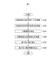
- FIG. 7 is a flowchart showing an example of processing in the inspection device.
- FIG. 1 is a diagram showing an example of an outline of a railway vehicle.
- FIG. 2 is a diagram conceptually showing the main directions of movement of the components of the railway vehicle.
- FIG. 3 is a diagram
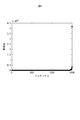
- FIG. 8 is a diagram showing an example of the distribution of eigenvalues of the autocorrelation matrix.
- FIG. 9 is a figure which shows an example of the time series data (measured value) of the measured value of the front-back direction force, and the time series data (calculated value) of the predicted value of the front-back direction force.
- FIG. 10 is a figure which shows an example of the time series data of the high frequency component of the front-back direction force.
- FIG. 11 is a diagram showing an example of the configuration of the inspection system.
- FIG. 12 is a diagram showing a calculation example, and is a diagram showing the curvature 1/R of the track from which the deviation amount is derived and the traveling speed of the railway vehicle.
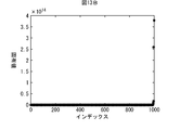
- FIG. 13A is a diagram showing a calculation example, and is a diagram showing a first example of the distribution of eigenvalues of the autocorrelation matrix R.
- FIG. 13B is a diagram showing a calculation example, and is a diagram showing a second example of the distribution of the eigenvalues of the autocorrelation matrix R.
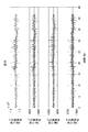
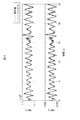
- FIG. 14 is a diagram showing a calculation example, and is a diagram showing time-series data of measured values of longitudinal force and time-series data of predicted values of longitudinal force.
- FIG. 15 is a diagram showing a calculation example, and is a diagram showing time-series data of high-frequency components of the longitudinal force.
- FIG. 16A is a diagram showing a calculation example according to the method of the first embodiment, and is a diagram showing a first example of the deviation amount y R.
- FIG. 16B is a diagram showing a calculation example by the method of the first embodiment, and is a diagram showing a second example of the deviation amount y R.
- FIG. 17A is a diagram showing a calculation example according to the method of the second embodiment, and is a diagram showing a first example of the deviation amount y R.
- FIG. 17B is a diagram showing a calculation example according to the method of the second embodiment, and is a diagram showing a first example of the deviation amount y R.
- FIG. 1 is a diagram showing an example of an outline of a railway vehicle.
- the railway vehicle travels in the positive direction of the x-axis (the x-axis is an axis along the traveling direction of the railway vehicle).
- the z-axis is assumed to be in the direction perpendicular to the track 16 (ground) (the height direction of the railway vehicle).
- the y-axis is assumed to be a horizontal direction perpendicular to the traveling direction of the railway vehicle (direction perpendicular to both the traveling direction and the height direction of the railway vehicle).
- rail vehicles are assumed to be business vehicles.
- the circles with a circle indicate the direction from the back side to the front side of the paper, and the circles with a circle indicate from the front side of the paper. The direction toward the back is shown.
- the railway vehicle has a vehicle body 11, bogies 12a and 12b, and wheel shafts 13a to 13d.
- a railroad vehicle in which one vehicle body 11 is provided with the two bogies 12a and 12b and the four wheel sets 13a to 13d will be described as an example.
- the wheel axles 13a to 13d have axles 15a to 15d and wheels 14a to 14d provided at both ends thereof.
- the carriages 12a and 12b are bolsterless carriages will be described as an example.
- the railroad vehicle has constituent elements other than the constituent elements shown in FIG. 1 (such as the constituent elements described in the equation of motion described later), but for convenience of notation, the constituent elements are not shown in FIG.
- the bogies 12a and 12b have bogie frames and pillow springs.
- axle boxes are arranged on both sides of each wheel axle 13a to 13d in the direction along the y-axis. Further, the bogie frame and the axle box are connected to each other by the axle box supporting device.
- the axle box support device is a device (suspension) arranged between the axle box and the bogie frame.
- the axle box support device absorbs the vibration transmitted from the track 16 to the railway vehicle. Further, the axle box supporting device suppresses movement of the axle box in the direction along the x axis and the direction along the y axis with respect to the bogie frame (preferably, such movement does not occur).
- the axle box is supported in a state in which its position with respect to the bogie frame is restricted.
- the axle box support devices are arranged on both sides of each wheel axle 13a to 13d in the direction along the y-axis. Since the railway vehicle itself can be realized by a known technique, its detailed description is omitted here.
- FIG. 2 is a diagram conceptually showing the main directions of movement of the components of the railway vehicle (the wheel sets 13a to 13d, the bogies 12a and 12b, the vehicle body 11).
- the x-axis, y-axis, and z-axis shown in FIG. 2 correspond to the x-axis, y-axis, and z-axis shown in FIG. 1, respectively.
- the wheel shafts 13a to 13d, the bogies 12a and 12b, and the vehicle body 11 rotate about the x axis as a rotation axis and move about the z axis as a rotation axis.
- a case of performing a motion along the y-axis will be described as an example.
- the motion of turning around the x-axis will be referred to as rolling, if necessary, and the turning direction around the x-axis will be referred to as the rolling direction, if necessary, along the x-axis.
- the direction will be referred to as the front-back direction as necessary.
- the front-rear direction is the traveling direction of the railway vehicle.
- the direction along the x-axis is the traveling direction of the railway vehicle.
- a motion of rotating about the z-axis as a rotating shaft is referred to as yawing as necessary
- a rotating direction about the z-axis as a rotating shaft is referred to as yawing direction as necessary
- a direction along the z-axis is required.
- the vertical direction is a direction perpendicular to the track 16.
- the motion along the y-axis is referred to as lateral vibration as necessary
- the direction along the y-axis is referred to as the left-right direction as necessary.
- the left-right direction is a direction that is perpendicular to both the front-rear direction (the traveling direction of the railway vehicle) and the up-down direction (the direction perpendicular to the track 16).
- the railway vehicle also performs other exercises, these exercises will not be taken into consideration in each embodiment for the sake of simplicity. However, these movements may be considered.
- FIG. 3 shows the measured and calculated values of the acceleration y t1 ⁇ in the lateral direction of the carriage 12a and the acceleration y w1 ⁇ , y w2 ⁇ in the lateral direction of the wheel axles 13a, 13b.
- the calculated value is an estimated value of the observed variable calculated by data assimilation.
- the horizontal axis of FIG. 3 is the elapsed time (seconds) from the reference time when the reference time is 0 (zero). Specifically, the horizontal axis of FIG. 3 represents the measurement time/calculation time of the acceleration y t1 ... In the lateral direction of the carriage 12a and the acceleration y w1 ..., Y w2 ... In the lateral direction of the wheel axles 13a and 13b.
- the estimated value of the state variable is derived so that the error between the value originally given as the measured value of the observation variable and the estimated value is the minimum or the expected value of the error is the minimum.
- the measured values of the accelerations y w1 ⁇ , y w2 ⁇ in the left-right direction of the wheel axles 13a, 13b and the measured values of the accelerations y t1 ⁇ , y t2 ⁇ in the lateral direction of the carriage 12a are It contains a lot of noise. From this, the present inventors have found that, depending on the state of the track 16 (railway), the estimated value does not approach the measured value and becomes a substantially constant value even if data assimilation is performed. This also applies to the lateral accelerations y w3 ..., Y w4 ... Of the wheel axles 13c, 13d, the lateral acceleration y t2 ...
- the present inventors significantly reduce the accuracy of the deviation amounts y R1 , y R2 , y R3 , y R4 without using the measured values of these accelerations when deriving the state variables. I thought that it could be derived without any effort.
- the amount of deviation is a formula based on the equation of motion that describes the motion of a railroad vehicle when traveling on a straight track, and is calculated using an expression that indicates the relationship between the amount of deviation and longitudinal force.
- the track 16 includes a straight line portion and a curved line portion.
- the straight line portion of the track 16 will be referred to as a straight line trajectory as necessary
- the curved portion of the track 16 will be referred to as a curved track as necessary.
- a state equation is constructed using a motion equation that describes the motion of a railroad vehicle traveling on a curved track when filtering by a filter (Kalman filter) that performs data assimilation
- the state variables may diverge. Therefore, the equation of state when filtering by a filter (Kalman filter) for data assimilation is constructed by using the equation of motion that describes the movement of a railroad vehicle traveling on a straight track.
- the equation of motion that describes the motion of a railway vehicle traveling on a curved track it is necessary to consider the centrifugal force that the railway vehicle receives during traveling. Therefore, the equation of motion that describes the motion of the railway vehicle traveling on the curved track includes a term including the radius of curvature of the rail.
- the inventors of the present invention have noticed that when a railroad vehicle travels on a curved track, the measured value of the longitudinal force has a certain bias compared to when it travels on a straight track.
- the component of the front-back direction force due to the passage is the same whether it is a curved track or a straight track. Therefore, the present inventors consider that the amount of deviation itself is irrelevant to the amount of the bias, and reduce the low frequency component (the behavior of the bias) from the time series data of the measured value of the longitudinal force.
- the calculation formula of the deviation amount is the same calculation formula whether it is a curved track or a straight track. Even if the design is a linear trajectory, it may actually have a curvature that affects the accuracy of estimating the deviation amount. Therefore, reducing not only low-frequency components (behavior of the bias) from the time-series data of the measured values of the longitudinal force contributes to the improvement of the accuracy of the deviation amount not only on the curved trajectory but also on the linear trajectory. .. In the description below, even if the trajectory is a linear trajectory by design, the trajectory having a curvature that affects the estimation accuracy of the deviation amount is actually a curved trajectory.
- Equation of motion an example of a motion equation that describes the motion of the railway vehicle will be described.
- the degree of freedom is not limited to 21 degrees of freedom. Increasing the degree of freedom improves the calculation accuracy but increases the calculation load. Further, the operation of the Kalman filter described below may become unstable. The degree of freedom can be appropriately determined in consideration of these points. Further, the following equations of motion represent movements of respective constituent elements (vehicle body 11, carriages 12a and 12b, wheel axles 13a to 13d) in respective directions (left-right direction, yawing direction, rolling direction), for example, Non-Patent Document 1 It can be realized by expressing it based on the description of 2. Therefore, an outline of each equation of motion will be described here, and detailed description will be omitted.
- the subscript w represents the wheel shafts 13a to 13d.
- a variable with a subscript w (only) is common to the wheel axles 13a to 13d.
- the subscripts w1, w2, w3, w4 represent the wheel sets 13a, 13b, 13c, 13d, respectively.
- the subscripts t and T represent the trucks 12a and 12b.
- Variables with subscripts t and T are common to the carriages 12a and 12b.
- the subscripts t1 and t2 represent the trucks 12a and 12b, respectively.
- the subscripts b and B represent the vehicle body 11.
- the subscript x represents the front-rear direction or the rolling direction
- the subscript y represents the horizontal direction
- the subscript z represents the vertical direction or the yawing direction.
- "..” and ".” added above the variables represent the second-order time differential and the first-order time differential, respectively.
- m w is the mass of the wheel shafts 13a to 13d.
- y w1 ⁇ (in the formula, ⁇ is attached on y w1 (hereinafter, the same applies to other variables)) is the acceleration in the left-right direction of the wheel shaft 13a.
- f 2 is a lateral creep coefficient (note that the lateral creep coefficient f 2 may be given for each of the wheel axles 13a to 13d).
- v is the traveling speed of the railway vehicle.
- y w1 ⁇ (in the formula, ⁇ is added above y w1 (hereinafter, the same applies to other variables)) is the speed of the wheel shaft 13a in the left-right direction.
- C wy is a damping constant in the left-right direction of the axle box supporting device that connects the axle box and the wheel axle.
- y t1 ⁇ is the speed of the carriage 12a in the left-right direction.
- a represents 1/2 of the distance in the front-rear direction between the wheel sets 13a, 13b, 13c, 13d provided on the trucks 12a, 12b (the wheel sets 13a, 13b, 13c, 13d provided on the trucks 12a, 12b). The distance between them is 2a).
- ⁇ t1 ⁇ is the angular velocity of the carriage 12a in the yawing direction.
- h 1 is the vertical distance between the center of the axle and the center of gravity of the carriage 12a.
- ⁇ t1 ⁇ is the angular velocity of the carriage 12a in the rolling direction.
- ⁇ w1 is the amount of rotation (angular displacement) of the wheel shaft 13a in the yawing direction.
- K wy is the spring constant of the axle box support device in the left-right direction.
- y w1 is the displacement of the wheel shaft 13a in the left-right direction.
- yt1 is the displacement of the carriage 12a in the left-right direction.
- ⁇ t1 is the amount of rotation (angular displacement) of the carriage 12a in the yawing direction.
- ⁇ t1 is the rotation amount (angular displacement) of the carriage 12a in the rolling direction.
- the variables in the expressions (2) to (4) are represented by replacing the variables in the expression (1) with the meaning of the subscripts described above.
- I wz is the moment of inertia of the wheel shafts 13a to 13d in the yawing direction. .psi..sub.w1 ... Is the angular acceleration of the wheel shaft 13a in the yawing direction.
- f 1 is a vertical creep coefficient.
- b is the distance in the left-right direction between the contact points between the two wheels attached to the wheel axles 13a to 13d and the track 16 (railway).
- ⁇ w1 ⁇ is the angular velocity of the wheel shaft 13 a in the yawing direction.
- C wx is a damping constant in the front-rear direction of the axle box supporting device.
- b 1 represents a half length of the interval in the left-right direction of the axle box support device (the interval in the left-right direction between the two axle box support devices provided on the left and right with respect to one wheel axle is 2b 1 ) .
- ⁇ is the tread slope.
- r is the radius of the wheels 14a to 14d.
- y R1 is the deviation amount at the position of the wheel shaft 13a.
- s a is an offset amount in the longitudinal direction from the center of the axle 15a ⁇ 15d to the axle box support spring.
- yt1 is the displacement of the carriage 12a in the left-right direction.
- K wx is a spring constant in the front-rear direction of the axle box supporting device.
- variables in the expressions (6) to (8) are represented by replacing the variables in the expression (5) with the meaning of the subscripts described above.
- y R2 , y R3 , and y R4 are deviation amounts at the positions of the wheel shafts 13b, 13c, and 13d, respectively.
- the deviation is a lateral displacement in the longitudinal direction of the rail, as described in Japanese Industrial Standards (JIS E 1001:2001).
- the amount of passage is the amount of displacement.
- 4A and 4B show an example of the deviation amount y R1 at the position of the wheel shaft 13a.
- FIG. 4A a case where the trajectory 16 is a linear trajectory will be described as an example.
- FIG. 4B a case where the trajectory 16 is a curved trajectory will be described as an example.
- 16a shows a rail and 16b shows a sleeper.
- FIG. 4A it is assumed that the wheel 14a of the wheel axle 13a is in contact with the rail 16a at the position 401.
- FIG. 4A it is assumed that the wheel 14a of the wheel axle 13a is in contact with the rail 16a at the position 401.
- the deviation amount y R1 at the position of the wheel axle 13a is the distance in the left-right direction between the contact position between the wheel 14a of the wheel axle 13a and the rail 16a and the position of the rail 16a in the case of assuming a normal state. ..
- the position of the wheel shaft 13a is a contact position between the wheel 14a of the wheel shaft 13a and the rail 16a.
- the deviation amounts y R2 , y R3 , y R4 at the positions of the wheel shafts 13b, 13c, 13d are also defined in the same manner as the deviation amount y R1 at the position of the wheel shaft 13a.
- m T is the mass of the trucks 12a and 12b.
- c'2 is a damping constant of the lateral movement damper.
- h 4 is the distance in the vertical direction between the center of gravity of the carriage 12a and the left/right moving damper.
- y b ⁇ is the speed of the vehicle body 11 in the left-right direction.
- L represents 1/2 of the distance between the centers of the carriages 12a and 12b in the front-rear direction (the distance between the centers of the carriages 12a and 12b in the front-rear direction is 2L).
- ⁇ b ⁇ is the angular velocity of the vehicle body 11 in the yawing direction.
- h 5 is the distance in the up-down direction between the left-right movement damper and the center of gravity of the vehicle body 11.
- ⁇ b ⁇ is the angular velocity of the vehicle body 11 in the rolling direction.
- y w2 ⁇ is the speed in the left-right direction of the wheel shaft 13b.
- k′ 2 is the spring constant of the air spring (pillow spring) in the left-right direction.
- h 2 is the vertical distance between the center of gravity of the carriages 12 a and 12 b and the center of the air spring (pillow spring).
- y b is the displacement of the vehicle body 11 in the left-right direction.
- ⁇ b is the amount of rotation (angular displacement) of the vehicle body 11 in the yawing direction.
- h 3 is a vertical distance between the center of the air spring (pillow spring) and the center of gravity of the vehicle body 11.
- ⁇ b is a rotation amount (angular displacement) of the vehicle body 11 in the rolling direction.
- Each variable in the expression (10) is represented by replacing the variable in the expression (9) with the meaning of the subscript described above.
- I Tz is the moment of inertia of the carriages 12a and 12b in the yawing direction.
- [psi t1 ⁇ ⁇ is the angular acceleration in the yawing direction of the carriage 12a.
- ⁇ w2 ⁇ is the angular velocity of the wheel shaft 13b in the yawing direction.
- ⁇ w2 is the rotation amount (angular displacement) of the wheel shaft 13b in the yawing direction.
- y w2 is the displacement of the wheel shaft 13b in the left-right direction.
- k'0 is a rubber bush rigidity of the yaw damper.
- b'0 is carriage 12a, two intervals in the lateral direction of the yaw damper which represents 1/2 of the interval in the horizontal direction of the two yaw damper, which is disposed on the left and right (carriage 12a, to 12b are disposed on the left and right with respect to 12b Becomes 2b' 0 ).
- ⁇ y1 is the rotation amount (angular displacement) in the yawing direction of the yaw damper arranged on the carriage 12a.
- k′′ 2 is a spring constant in the front-rear direction of the air spring (pillow spring).
- b 2 represents 1/2 of the distance in the left-right direction between the two air springs (pillow springs) arranged on the left and right sides of the carriages 12a and 12b (the two air springs arranged on the left and right sides of the carriages 12a and 12b). (The distance between the pillow springs in the left-right direction is 2b 2. )
- Each variable in the equation (12) is represented by replacing the variable in the equation (11) with the meaning of the subscript described above.
- ITx is the moment of inertia of the carriages 12a and 12b in the rolling direction.
- c 1 is a vertical damping constant of the shaft damper.
- b'1 is trolley 12a, the right and left directions of the two axes dampers representing 1/2 of the interval in the lateral direction of the two axes damper which is disposed on the left and right (carriage 12a, to 12b are disposed on the left and right with respect to 12b interval becomes 2b' 1 in).
- c 2 is a vertical damping constant of the air spring (pillow spring).
- ⁇ a1 ⁇ is an angular velocity in the rolling direction of the air spring (pillow spring) arranged on the carriage 12a.
- k 1 is the vertical spring constant of the axial spring.
- ⁇ is a value obtained by dividing the volume of the main body of the air spring (pillow spring) by the volume of the auxiliary air chamber.
- k 2 is the spring constant of the air spring (pillow spring) in the vertical direction.
- ⁇ a1 is a rotation amount (angular displacement) in the rolling direction of the air spring (pillow spring) arranged on the carriage 12a.
- k 3 is an equivalent rigidity due to a change in the effective pressure receiving area of the air spring (pillow spring).
- ⁇ a2 is the rotation amount (angular displacement) in the rolling direction of the air spring (pillow spring) arranged on the carriage 12b.
- m B is the mass of the carriages 12a and 12b.
- y b ... Is the acceleration in the left-right direction of the vehicle body 11.
- y t2 ⁇ is the speed of the carriage 12b in the left-right direction.
- ⁇ t2 ⁇ is the angular velocity of the carriage 12b in the rolling direction.
- y t2 is the displacement of the carriage 12b in the left-right direction.
- ⁇ t2 is the rotation amount (angular displacement) of the carriage 12b in the rolling direction.
- I Bz is the moment of inertia of the vehicle body 11 in the yawing direction.
- ⁇ b ⁇ is an angular acceleration of the vehicle body 11 in the yawing direction.
- c 0 is a damping constant in the front-rear direction of the yaw damper.
- ⁇ y1 ⁇ is the angular velocity in the yawing direction of the yaw damper arranged on the carriage 12 a.
- ⁇ y2 ⁇ is the angular velocity in the yawing direction of the yaw damper arranged on the carriage 12b.
- ⁇ t2 is a rotation amount (angular displacement) of the carriage 12b in the yawing direction.
- I Bx is the moment of inertia of the vehicle body 11 in the rolling direction.
- ⁇ b is the angular acceleration of the vehicle body 11 in the rolling direction.
- ⁇ y2 is the rotation amount (angular displacement) in the yawing direction of the yaw damper arranged on the carriage 12b.
- ⁇ a2 ⁇ is an angular velocity in the rolling direction of the air spring (pillow spring) arranged on the carriage 12b.
- the longitudinal force itself is the same as that described in Patent Document 1.
- the in-phase component of the vertical creep force of one of the left and right wheels of the one wheel axle and the vertical creep force of the other wheel is a component corresponding to the braking force or the driving force. Therefore, it is preferable to determine the longitudinal force so as to correspond to the antiphase component of the longitudinal creep force.
- the anti-phase component of the longitudinal creep force is a component in which the longitudinal creep force of one of the left and right wheels of one wheel axle and the longitudinal creep force of the other wheel have mutually opposite phases. That is, the antiphase component of the vertical creep force is the component of the vertical creep force in the direction of twisting the axle.
- the front-rear direction force is a component having a phase opposite to each other among the front-rear direction components of the forces generated in the two members attached to the left and right sides of one wheel axle.
- the axle box support device is a monolink type axle box support device
- the axle box support device includes a link
- the axle box and the bogie frame are connected by the link. Rubber bushes are attached to both ends of this link.
- the front-rear direction force is a component having opposite phases to each other in the front-rear direction component of the load received by each of the two links attached to the left and right ends of one wheel axle.
- the links mainly receive the load in the front-back direction among the loads in the front-back direction, the left-right direction, and the vertical direction.
- one strain gauge may be attached to each link.
- the longitudinal component of the load received by the link is derived to obtain the measured value of the longitudinal force.
- the displacement of the rubber bush attached to the link in the front-rear direction may be measured by a displacement meter.
- the product of the measured displacement and the spring constant of the rubber bush is used as the measured value of the longitudinal force.
- the load measured by the strain gauge attached to the link may include not only the front-back direction component but also at least one of the left-right direction component and the up-down direction component.
- the load of the component in the horizontal direction and the load of the component in the vertical direction received by the link are sufficiently smaller than the load in the component in the front-rear direction. Therefore, only by attaching one strain gauge to each link, it is possible to obtain a measured value of the front-rear direction force having an accuracy required for practical use.
- the measured value of the front-back direction force may include components other than the front-back direction component. Therefore, three or more strain gauges may be attached to each link so that the strains in the vertical and horizontal directions are canceled. By doing so, the accuracy of the measured value of the front-back direction force can be improved.
- the axle box support device is an axle beam type axle box support device
- the axle box support device includes an axle beam
- the axle box and the bogie frame are connected by the axle beam.
- the axle beam may be formed integrally with the axle box.
- a rubber bush is attached to the end of the axle beam on the bogie frame side.
- the front-rear direction force is a component in the front-rear direction component of the load received by each of the two axle beams attached to each of the left and right ends of the one wheel axle, and the components having opposite phases.
- the shaft beam is likely to receive the load in the left-right direction in addition to the load in the front-rear direction among the loads in the front-rear direction, the left-right direction, and the vertical direction.
- two or more strain gauges are attached to each shaft beam so that the strain in the left-right direction is canceled.
- the measured values of these strain gauges are used to derive the longitudinal component of the load applied to the axial beam to obtain the measured longitudinal force.
- the displacement of the rubber bush attached to the shaft beam in the front-rear direction may be measured by a displacement meter.
- the product of the measured displacement and the spring constant of the rubber bush is used as the measured value of the longitudinal force.
- the axle box support device is an axle beam type axle box support device
- the aforementioned member for supporting the axle box is an axle beam or a rubber bush.
- the load measured by the strain gauge attached to the shaft beam may include not only components in the front-rear direction and left-right direction but also components in the up-down direction.
- the vertical component load received by the shaft beam is sufficiently smaller than the longitudinal component load and the lateral component load. .. Therefore, even if the strain gauge is not attached so as to cancel the load of the component in the vertical direction received by the axial beam, it is possible to obtain the measured value of the longitudinal force having the accuracy required for practical use.
- the measured longitudinal force may include components other than the longitudinal component, and three or more strain gauges may be added to cancel the vertical strain in addition to the horizontal strain. May be attached to each shaft beam. By doing so, the accuracy of the measured value of the front-back direction force can be improved.
- the axle box support device is a leaf spring type axle box support device
- the axle box support device is provided with a leaf spring
- the axle box and the bogie frame are connected by the leaf spring.
- a rubber bush is attached to the end of the leaf spring.
- the front-rear direction force is a component having opposite phases to each other in the front-rear direction component of the load received by each of the two leaf springs attached to the left and right ends of one wheel axle.
- the leaf springs are likely to receive the load in the left-right direction and the load in the up-down direction in addition to the load in the front-rear direction among the loads in the front-rear direction, the left-right direction, and the vertical direction.
- the axle box support device is a leaf spring type axle box support device
- the aforementioned member for supporting the axle box is a leaf spring or a rubber bush.
- a known laser displacement gauge or an eddy current displacement gauge can be used as the displacement gauge described above.
- the front-back direction force has been described by exemplifying the case where the system of the axle box supporting device is the monolink type, the shaft beam type, and the leaf spring type.
- the system of the axle box supporting device is not limited to the monolink type, the shaft beam type, and the leaf spring type.
- the longitudinal force can be determined similarly to the monolink type, the axial beam type, and the leaf spring type.
- the case where one measured value of the front-rear direction force is obtained for one wheel axle will be described as an example. That is, the railway vehicle shown in FIG. 1 has four wheel axles 13a to 13d. Therefore, the measured values of the four longitudinal forces T 1 to T 4 are obtained.
- FIG. 5 is a diagram showing an example of a functional configuration of the inspection device 500.
- FIG. 6 is a diagram illustrating an example of a hardware configuration of the inspection device 500.
- FIG. 7 is a flowchart showing an example of processing in the inspection device 500.
- the case where the inspection device 500 is mounted on a railway vehicle is shown as an example.
- the inspection device 500 has, as its functions, a storage unit 501, a data acquisition unit 502, a first frequency adjustment unit 503, a state variable derivation unit 504, a second frequency adjustment unit 505, an orbit state derivation unit 506, And an output unit 507.
- the inspection device 500 includes a CPU 601, a main storage device 602, an auxiliary storage device 603, a communication circuit 604, a signal processing circuit 605, an image processing circuit 606, an I/F circuit 607, a user interface 608, a display 609, and a bus. 610.
- the CPU 601 controls the inspection device 500 as a whole.
- the CPU 601 executes the program stored in the auxiliary storage device 603 by using the main storage device 602 as a work area.
- the main storage device 602 temporarily stores data.
- the auxiliary storage device 603 stores various data in addition to the program executed by the CPU 601.
- the auxiliary storage device 603 stores a state equation and an observation equation described later.
- the storage unit 501 is realized by using the CPU 601 and the auxiliary storage device 603, for example.
- the communication circuit 604 is a circuit for communicating with the outside of the inspection device 500.
- the communication circuit 604 receives, for example, information on the measured value of the front-back direction force.
- the communication circuit 604 may perform wireless communication or wired communication with the outside of the inspection apparatus 500.
- the communication circuit 604 is connected to an antenna provided in a railway vehicle when performing wireless communication.
- the signal processing circuit 605 performs various kinds of signal processing on the signal received by the communication circuit 604 and the signal input under the control of the CPU 601.
- the data acquisition unit 502 is realized by using the CPU 601, the communication circuit 604, and the signal processing circuit 605, for example.
- the first frequency adjusting unit 503, the state variable deriving unit 504, the second frequency adjusting unit 505, and the trajectory state deriving unit 506 are realized by using the CPU 601 and the signal processing circuit 605, for example.
- the image processing circuit 606 performs various kinds of image processing on the signal input under the control of the CPU 601.
- the signal subjected to this image processing is output to the display 609.
- the user interface 608 is a part where the operator gives an instruction to the inspection apparatus 500.
- the user interface 608 has, for example, buttons, switches, dials, and the like. Further, the user interface 608 may have a graphical user interface using the display 609.
- the display 609 displays an image based on the signal output from the image processing circuit 606.
- the I/F circuit 607 exchanges data with a device connected to the I/F circuit 607.
- a user interface 608 and a display 609 are shown as devices connected to the I/F circuit 607.
- the device connected to the I/F circuit 607 is not limited to these.
- a portable storage medium may be connected to the I/F circuit 607.
- at least a part of the user interface 608 and the display 609 may be outside the inspection device 500.
- the output unit 507 is realized, for example, by using at least one of the communication circuit 604 and the signal processing circuit 605, the image processing circuit 606, the I/F circuit 607, and the display 609.
- the CPU 601, the main storage device 602, the auxiliary storage device 603, the signal processing circuit 605, the image processing circuit 606, and the I/F circuit 607 are connected to the bus 610. Communication between these components is done via bus 610. Further, the hardware of the inspection device 500 is not limited to that shown in FIG. 6 as long as the functions of the inspection device 500 described later can be realized.
- the storage unit 501 stores an equation used by the state variable derivation unit 504 described below to derive a state variable.
- the storage unit 501 stores the state equation and the observation equation.
- the case of using the state equation and the observation equation described in Patent Document 1 will be described as an example.
- the state equation is constructed as follows without including the equations (5) to (8) (the equation of motion describing the yawing of the wheel axles 13a to 13d) in the state equation.
- equations (9) and (10) (equation of motion describing lateral vibration (movement in the left-right direction) of the carriages 12a and 12b) and equations (13) and (14) (rolling of the carriages 12a and 12b) are described.
- Equations (20) and (21) (equation of motion describing the rolling of the air spring (pillow spring) arranged on the carriage 12a and the air spring (pillow spring) arranged on the carriage 12b) are used as they are.
- equations (1) to (4) (equation of motion describing lateral vibration (motion in the left-right direction) of the wheel axles 13a to 13d) and equations (11) and (12) (yawing of the bogies 12a and 12b)
- the described equation of motion includes the rotation amounts (angular displacements) ⁇ w1 to ⁇ w4 and the angular velocities ⁇ w1 ⁇ to ⁇ w4 ⁇ of the wheel shafts 13 a to 13 d in the yawing direction. Equations (1) to (4), (11), and (12) are obtained by eliminating these variables to form a state equation.
- the longitudinal forces T 1 to T 4 on the wheel shafts 13a to 13d are expressed by the following equations (22) to (25).
- the longitudinal forces T 1 to T 4 depend on the difference between the angular displacements ⁇ w1 to ⁇ w4 of the wheel axle in the yawing direction and the angular displacements ⁇ t1 to ⁇ t2 of the bogie on which the wheel axle is provided. Determined.
- the conversion variables e 1 to e 4 are defined as in Expressions (26) to (29) below. In this way, the conversion variables e 1 to e 4 are defined by the difference between the angular displacements ⁇ t1 to ⁇ t2 of the bogie in the yawing direction and the angular displacements ⁇ w1 to ⁇ w4 of the wheel axle in the yawing direction.
- the conversion variables e 1 to e 4 are variables for mutually converting the angular displacements ⁇ t1 to ⁇ t2 of the carriage in the yawing direction and the angular displacements ⁇ w1 to ⁇ w4 of the wheel axle in the yawing direction.
- the equations (11) and (12) (the equation of motion describing the yawing of the bogies 12a and 12b) are expressed by using the longitudinal forces T 1 to T 4 to be included in the equations of motion.
- the angular displacement ⁇ w1 ⁇ ⁇ w4 and the angular velocity ⁇ w1 ⁇ ⁇ ⁇ w4 ⁇ in the yawing direction of which was Wajiku 13a ⁇ 13d may be erased.
- Equation 39 represents the equation of motion that describes the yawing of the carriages 12a and 12b.
- a state equation is constructed using the equations (34) to (39).
- equations (40) to (43) are ordinary differential equations.
- the actual values of the conversion variables e 1 to e 4 which are the solutions of the ordinary differential equation, can be obtained by using the values of the longitudinal forces T 1 to T 4 on the wheel shafts 13a to 13d.
- the values of the front-rear direction forces T 1 to T 4 are caused by the first frequency adjusting unit 503, which will be described later, from the fact that the railroad vehicle travels on the curved portion of the track from the time-series data of the measured values of the front-rear direction force.
- the signal strength of the low frequency component generated by the above is reduced.
- the actual values of the conversion variables e 1 to e 4 thus obtained are given to the equations (34) to (37). Further, the values of the longitudinal forces T 1 to T 4 on the wheel shafts 13a to 13d are given to the equations (38) and (39).
- the values of the front-rear direction forces T 1 to T 4 are caused by the first frequency adjusting unit 503, which will be described later, from the fact that the railroad vehicle travels on the curved portion of the track from the time-series data of the measured values of the front-rear direction force. The signal strength of the low frequency component generated by the above is reduced.
- equation (44) the variables shown in the following equation (44) are used as state variables, and the movements of the equations (9), (10), (13) to (21), and (34) to (39) are used. Construct equations of state using equations.
- the storage unit 501 inputs and stores, for example, the state equation configured as described above based on the operation of the user interface 608 by the operator.
- the left and right accelerations of the vehicle body 11, the left and right accelerations of the carriages 12a and 12b, and the left and right accelerations of the wheel axles 13a to 13d are used as observation variables.
- This observation variable is an observation variable for filtering by the Kalman filter described later.
- the observation equation is constructed using the equations (34) to (37), (9), (10), and (15) (motion equation describing lateral vibration).
- the storage unit 501 inputs, for example, the observation equation thus configured based on the operation of the user interface 608 by the operator and stores it.
- the derivation unit 506 and the output unit 507 are activated. That is, the process according to the flowchart of FIG. 7 starts after the state equation and the observation equation are stored in the inspection device 500.
- the data acquisition unit 502 acquires time-series data of measured values of the front-back direction force.
- the method of measuring the longitudinal force is as described above.
- the data acquisition unit 502 communicates with a computing device that computes the longitudinal force using the measured value of the strain gauge for measuring the longitudinal force, for example, to obtain time-series data of the longitudinal force measurement value. Can be obtained.
- the data acquisition unit 502 uses the time-series data of the measured values of the acceleration of the vehicle body 11 in the left-right direction, the time-series data of the measured values of the acceleration of the carts 12a and 12b in the left-right direction, and the acceleration of the wheel axles 13a to 13d in the left-right direction. Do not acquire the time series data of the measured value of.
- the first frequency adjustment unit 503 reduces (preferably removes) the signal strength of the low frequency component included in the time series data of the measured values of the longitudinal force acquired by the data acquisition unit 502.
- This low-frequency component signal is not measured when the railway vehicle is traveling on a straight track having a curvature of 0 (zero), but is measured when the railway vehicle is traveling on a curved track. Is. That is, the signal measured when the railroad vehicle is traveling on a curved track is the signal measured when the railroad vehicle is traveling on a straight track with a curvature of 0 (zero). It can be regarded as a signal in which signals are superimposed.
- the present inventors have devised a model in which an auto-regressive model (AR (Auto-regressive) model) is modified. Then, the present inventors have conceived to use this model to reduce the signal strength of the low frequency component included in the time series data of the measured value of the longitudinal force.
- AR Auto-regressive
- the model devised by the present inventors will be referred to as a modified autoregressive model.
- a known autoregressive model is simply called an autoregressive model.
- an example of the modified autoregressive model will be described.
- the value of the time series data of the physical quantity y at time k (1 ⁇ k ⁇ M) is y k .
- M is a number indicating up to what time the time series data of the physical quantity y includes data, and is set in advance.
- the time series data of the physical quantity will be abbreviated as data y as necessary.
- An autoregressive model approximating the value y k of the data y is, for example, as shown in the following expression (45).
- the autoregressive model means that the predicted value y ⁇ k of the physical quantity at the time k (m+1 ⁇ k ⁇ M) in the data y is the time k ⁇ before the time k ⁇ in the data y. It is an expression represented by using the actual value y kl of the physical quantity of l (1 ⁇ l ⁇ m).
- y ⁇ k is expressed by adding ⁇ on yk in the equation (45).
- ⁇ in the equation (45) is a coefficient of the autoregressive model.
- m is a number of values of the data y to be used to approximate the value y k of the data y at time k in the autoregressive model, the time k-1 ⁇ k-m of consecutive before that time k Is the number of values y k ⁇ 1 to y k ⁇ m of the data y.
- m is an integer less than M. For example, 1500 can be used as m.
- the least squares method is used to find a conditional expression for approximating the predicted value y ⁇ k of the physical quantity at the time k by the autoregressive model to the value y k .
- a condition for the predicted value y ⁇ k of the physical quantity at the time k by autoregressive model approximates a value y k for example, square errors between the predicted value y ⁇ k value y k of the physical quantity at the time k by autoregressive model Can be adopted. That is, using the least squares method to approximate the predicted value y ⁇ k of the physical quantity at the time k by autoregressive model to a value y k.
- the following expression (46) is a conditional expression for minimizing the squared error between the predicted value y ⁇ k of the physical quantity at the time k by the autoregressive model and the value y k .
- R jl in the equation (48) is called autocorrelation of the data y, and is a value defined by the following equation (49).
- at this time is called the time difference.
- Equation (50) derived from the condition that minimizes the prediction value y ⁇ k of the physical quantity at the time k by autoregressive model, the value y k of the physical quantity at the time k corresponding to the predicted value y ⁇ k, the error Is the equation
- the equation (50) is called the Yule-Walker equation.
- the equation (50) is a linear equation in which a vector consisting of the coefficients of the autoregressive model is a variable vector.
- the constant vector on the left side of the equation (50) is a vector whose component is the autocorrelation of the data y with a time difference of 1 to m.
- the constant vector on the left side of the equation (50) will be referred to as an autocorrelation vector as necessary.
- the coefficient matrix on the right side of the equation (50) is a matrix whose component is the autocorrelation of the data y with a time difference of 0 to m-1.
- the coefficient matrix on the right side of Expression (50) will be referred to as an autocorrelation matrix as necessary.
- the coefficient ⁇ is derived so that the predicted value y ⁇ k of the physical quantity at the time k derived by the autoregressive model is as close as possible to the value y k of the physical quantity at the time k. Therefore, the frequency characteristic of the autoregressive model includes many frequency components included in the value y k of the data y at each time.
- the present inventors paid their attention to the autocorrelation matrix R by which the coefficient ⁇ of the autoregressive model is multiplied, and diligently studied. As a result, the present inventors have found that the influence of high frequency components included in the data y can be reduced by using a part of the eigenvalues of the autocorrelation matrix R. That is, the present inventors have found that the autocorrelation matrix R can be rewritten so that the low frequency component is emphasized.
- the diagonal matrix ⁇ of the equation (52) is a matrix whose diagonal components are the eigenvalues of the autocorrelation matrix R, as shown in the following equation (53).
- the diagonal components of the diagonal matrix ⁇ are ⁇ 11 , ⁇ 22 ,..., ⁇ mm .
- the orthogonal matrix U is a matrix in which each column component vector becomes an eigenvector of the autocorrelation matrix R.
- the column component vectors of the orthogonal matrix U are u 1 , u 2 ,..., U m .
- the eigenvalue of the autocorrelation matrix R with respect to the eigenvector u j is ⁇ jj .
- the eigenvalue of the autocorrelation matrix R is a variable that reflects the intensity of each frequency component included in the time waveform of the physical quantity predicted value y ⁇ k at time k by the autoregressive model.
- ⁇ 11 , ⁇ 22 ,..., ⁇ mm which are the diagonal components of the diagonal matrix ⁇ obtained from the result of the singular value decomposition of the autocorrelation matrix R, are in descending order in order to simplify the notation of the mathematical expression.
- the matrix R′ is defined as in equation (54) below, using s eigenvalues starting from the largest one. s is a number of 1 or more and less than m. In this embodiment, s is predetermined.
- the matrix R′ is a matrix that approximates the autocorrelation matrix R using s eigenvalues of the eigenvalues of the autocorrelation matrix R.
- the matrix U s in the equation (54) is an m ⁇ s matrix configured by s column component vectors (eigenvectors corresponding to the eigenvalues used) from the left of the orthogonal matrix U in the equation (52). That is, the matrix U s is a partial matrix formed by cutting out the left m ⁇ s elements from the orthogonal matrix U.
- U s T in the equation (54) is a transposed matrix of U s .
- U s T is an s ⁇ m matrix composed of s row component vectors from the top of the matrix U T of the equation (52).
- the matrix ⁇ s in the equation (54) is an s ⁇ s matrix configured by s columns from the left and s rows from the top of the diagonal matrix ⁇ in the equation (52). That is, the matrix ⁇ s is a partial matrix configured by cutting out the upper left s ⁇ s element from the diagonal matrix ⁇ . If the matrix ⁇ s and the matrix U s are expressed by matrix elements, the following expression (55) is obtained.
- the following equation (57) is obtained as an equation for obtaining the coefficient ⁇ .
- the “corrected autoregressive model” is a model for calculating the predicted value y ⁇ k of the physical quantity at the time k by the equation (45) using the coefficient ⁇ obtained by the equation (57).
- the matrix U s is not a submatrix formed by cutting out the left m ⁇ s elements from the orthogonal matrix U, but is formed by cutting out a column component vector (eigenvector) corresponding to the eigenvalue used. Becomes a submatrix.
- the matrix ⁇ s is not a sub-matrix formed by cutting out the upper left s ⁇ s element from the diagonal matrix ⁇ , but the eigenvalues used to determine the coefficients of the modified autoregressive model are diagonal elements. It becomes a submatrix cut out into.
- Equation (57) is an equation used to determine the coefficient of the modified autoregressive model.
- the matrix U s of the expression (57) is a submatrix of the orthogonal matrix U obtained by singular value decomposition of the autocorrelation matrix R, and the eigenvectors corresponding to the eigenvalues used to determine the coefficients of the modified autoregressive model are listed. It is a matrix (third matrix) used as a component vector.
- the matrix ⁇ s of Expression (57) is a partial matrix of the diagonal matrix obtained by singular value decomposition of the autocorrelation matrix R, and the eigenvalues used to determine the coefficients of the modified autoregressive model are the diagonal components. Is a matrix (second matrix).
- the matrix U s ⁇ s U s T of the expression (57) is a matrix (first matrix) derived from the matrix ⁇ s and the matrix U s .
- the coefficient ⁇ of the modified autoregressive model is obtained by calculating the right side of the expression (57).
- the method of deriving the coefficient ⁇ of the modified autoregressive model which is the basis of the modified autoregressive model, is the method of using the least squares method for the predicted value y ⁇ k of the physical quantity at the time k so that it can be intuitively understood. ..
- a method of defining an autoregressive model using the concept of stochastic process and deriving its coefficient In that case, the autocorrelation is represented by the autocorrelation of the stochastic process (population).
- the autocorrelation of this stochastic process is expressed as a function of the time difference. Therefore, the autocorrelation of the data y in this embodiment may be replaced with a value calculated by another calculation formula as long as it approximates the autocorrelation of the stochastic process.
- R 22 to R mm are autocorrelations with a time difference of 0 (zero), but they may be replaced with R 11 .
- the number s of eigenvalues extracted from the autocorrelation matrix R shown in Expression (53) can be determined, for example, from the distribution of the eigenvalues of the autocorrelation matrix R.
- the physical quantity in the description of the modified autoregressive model described above is the longitudinal force.
- the value of the longitudinal force fluctuates according to the condition of the rail vehicle. Therefore, first, the railway vehicle is run on the track 16 to obtain data y regarding the measured value of the longitudinal force.
- An autocorrelation matrix R is obtained using the equations (49) and (51) for each of the obtained data y.
- the eigenvalues of the autocorrelation matrix R are obtained by performing singular value decomposition represented by the equation (52) on the autocorrelation matrix R.
- FIG. 8 is a diagram showing an example of the distribution of eigenvalues of the autocorrelation matrix R.
- the eigenvalues ⁇ 11 to ⁇ mm obtained by singular value decomposition of the autocorrelation matrix R for each of the time series data of the measured value y of the longitudinal force T 1 on the wheel axle 13a are rearranged in ascending order, I'm plotting.
- the horizontal axis of FIG. 8 is the index of the eigenvalue, and the vertical axis is the value of the eigenvalue.
- the first frequency adjustment unit 503 performs the following processing each time the data acquisition unit 502 acquires the value y k at time k of the time series data of the measured value y of the longitudinal force in a predetermined sampling cycle. First, the first frequency adjusting unit 503 calculates the equations (49) and (51) based on the time-series data of the measured value y of the front-back direction force and the preset numbers M and m. To generate an autocorrelation matrix R.
- the first frequency adjusting unit 503 derives the orthogonal matrix U and the diagonal matrix ⁇ of equation (52) by performing singular value decomposition on the autocorrelation matrix R, and the autocorrelation matrix R is calculated from the diagonal matrix ⁇ .
- the eigenvalues ⁇ 11 to ⁇ mm of are derived.
- the first frequency adjusting unit 503 calculates the s eigenvalues ⁇ 11 to ⁇ ss of the largest eigenvalues ⁇ 11 to ⁇ mm of the autocorrelation matrix R from the largest eigenvalues ⁇ 11 to ⁇ ss , and determines the coefficient ⁇ Is selected as the eigenvalue of the autocorrelation matrix R used to obtain
- the first frequency adjustment unit 503 uses the coefficient ⁇ of the modified autoregressive model and the time series data of the measured value y of the front-back direction to calculate the measured value y of the front-back direction according to the equation (45).
- a prediction value y ⁇ k at time k of the time series data of is derived.
- the time-series data of the predicted value y ⁇ k of the front-rear direction force is time-series data obtained by extracting the low-frequency component included in the time-series data of the measured value y of the front-rear direction force.
- FIG. 9 is a figure which shows an example of the time series data (measured value) of the measured value of the front-back direction force, and the time series data (calculated value) of the predicted value of the front-back direction force.
- the measured values of the four longitudinal forces T 1 to T 4 are obtained. That is, four pieces of data y are obtained for the longitudinal force.
- FIG. 9 shows measured values and calculated values for each of these four data y.
- the horizontal axis of FIG. 9 is the elapsed time (seconds) from the reference time when the reference time is 0 (zero), and represents the measurement time/calculation time of the longitudinal forces T 1 to T 4 .
- the vertical axis represents the longitudinal forces T 1 to T 4 (Nm).
- the calculated value of the front-rear direction force T 1 on the wheel axle 13a is biased in about 15 seconds to 35 seconds. That is, the calculated value of the front-rear direction force T 1 on the wheel axle 13a is a value larger than the other time in about 15 seconds to 35 seconds. This period corresponds to the period in which the wheel axle 13a passes through the curved track.
- the calculated values of the front-rear direction force T 2 on the wheel shaft 13b, the calculated values of the front-rear direction force T 3 on the wheel shaft 13c, and the calculated values of the front-rear direction force T 4 on the wheel shaft 13d are also calculated values of the front-rear direction force T 1 on the wheel shaft 13a.
- the wheel axles 13b, 13c and 13d are biased during the passage of the curved track.
- wheel sets 13a ⁇ 13d is a curved track It is possible to remove low frequency components due to passage. That is, in FIG. 9, except the calculated value from the measured values of the longitudinal force T 1 ⁇ T 4 in axle 13a ⁇ 13d, the longitudinal direction forces T 1 ⁇ T 4 when the wheel shaft 13a ⁇ 13d has passed the curved track A longitudinal force equivalent to that when the wheel shafts 13a to 13d pass a straight track can be obtained.
- the first frequency adjusting unit 503 subtracts the time-series data of the predicted value y ⁇ k of the longitudinal force from the time-series data (data y) of the measured value y k of the longitudinal force.
- the time series data obtained by subtracting the time series data of the predicted value y ⁇ k of the front-back direction force from the time series data (data y) of the measured value y k of the front-back direction force is used in the front-back direction as necessary. This is called time series data of high frequency components of force.
- the value at each sampling time of the time series data of the high frequency component of the front-rear direction force is referred to as the value of the high frequency component of the front-rear direction force as necessary.
- FIG. 10 is a figure which shows an example of the time series data of the high frequency component of the front-back direction force.
- the vertical axis of FIG. 10 shows time-series data of high-frequency components of the longitudinal forces T 1 , T 2 , T 3 , and T 4 . That is, the high frequency component of the longitudinal force T 1, T 2, T 3 , T 4 indicated on the vertical axis of FIG. 10, respectively, shown in FIG. 9, axle 13a, 13b, 13c, anteroposterior 13d directed force T 1 , T 2 , T 3 , and T 4 are obtained by subtracting the calculated values from the measured values.
- the horizontal axis of FIG. 10 is, similarly to the horizontal axis of FIG.
- the first frequency adjusting unit 503 derives the time-series data of the high frequency components of the front-rear direction forces T 1 to T 4 as described above.
- the state variable deriving unit 504 uses the Kalman filter as the observation equation stored in the storage unit 501 as the observation equation, and the state equation stored in the storage unit 501 as the state equation stored in the storage unit 501. decide. At this time, the state variable deriving unit 504 uses the time-series data of the high frequency components of the front-rear direction forces T 1 to T 4 generated by the first frequency adjusting unit 503. In the present embodiment, when determining the estimated value of the state variable, time-series data of measured values of acceleration of the vehicle body 11 in the left-right direction, time-series data of measured values of acceleration of the carts 12a and 12b in the left-right direction, and the wheel axle. Of the time-series data of the acceleration measurement values in the left-right direction of 13a to 13d, at least the time-series data in the period in which the measurement values of the longitudinal forces T 1 to T 4 are obtained are not used.
- the Kalman filter is one of the methods for data assimilation. That is, the Kalman filter is an example of a method of determining an estimated value of an unobserved variable (state variable) so that the difference between the measured value and the estimated value of an observable variable (observed variable) becomes small (minimum). ..
- the state variable deriving unit 504 obtains a Kalman gain that makes the difference between the measured value and the estimated value of the observed variable small (minimum), and obtains the estimated value of the unobserved variable (state variable) at that time.
- X ⁇ ⁇ X+W ⁇ (59)
- Equation (58) Y is a vector that stores the measured value of the observed variable.
- H is an observation model.
- X is a vector that stores state variables.
- V is the observation noise.
- X ⁇ represents the time derivative of X.
- ⁇ is a linear model.
- W is system noise. Since the Kalman filter itself can be realized by a known technique, its detailed description will be omitted.
- a measurement value (a measurement value of acceleration in the left-right direction of the vehicle body 11, a measurement value of acceleration in the left-right direction of the carriages 12a and 12b, and a wheel axle 13a...
- the measurement value of the acceleration in the horizontal direction of 13d) is used as it is.
- the value originally given as the measurement value of the observation variable at the time of data assimilation is not a measurement value but a preset value.
- the average value of the time series data of acceleration is 0 (zero)
- all constant values given as observation variables are set to 0 (zero).
- the state variable derivation unit 504 minimizes the error of the estimated value of the observation variable with respect to a constant value (here, 0 (zero)) or the expected value of the error when performing data assimilation.
- the estimated value of the state variable is derived so that The state variable derivation unit 504 generates time series data of the estimated value of the state variable shown in the equation (44) by determining the estimated value of the state variable shown in the equation (44) at a predetermined sampling cycle.
- the first frequency adjusting unit 503 uses the autocorrelation matrix R shown in the equation (53) so that the signal intensity of the low-frequency component included in the time series data of the measured value of the longitudinal force is sufficiently removed.
- the process of the second frequency adjusting unit 505 is unnecessary.
- the second frequency adjusting unit 505 uses the modified autoregressive model, similarly to the first frequency adjusting unit 503, and outputs the signal of the low frequency component included in the time series data of the estimated value of the state variable. Reduce strength.
- the second frequency adjusting unit 505 performs the following processing for each state variable at a predetermined sampling cycle.
- the physical quantity in the above description of the modified autoregressive model becomes a state variable. That is, the state variable data y becomes time series data of the estimated value of the state variable generated by the state variable derivation unit 504.
- Each of the estimated values of the state variables fluctuates according to the state of the railway vehicle.
- the second frequency adjusting unit 505 uses the equations (49) and (51) based on the estimated value data y of the state variable and the preset numbers M and m. Generate a correlation matrix R.
- the second frequency adjusting unit 505 derives the orthogonal matrix U and the diagonal matrix ⁇ of equation (52) by performing singular value decomposition on the autocorrelation matrix R, and calculates the autocorrelation matrix R from the diagonal matrix ⁇ .
- the eigenvalues ⁇ 11 to ⁇ mm of are derived.
- the second frequency adjusting unit 505 determines s eigenvalues ⁇ 11 to ⁇ ss from the largest of the plurality of eigenvalues ⁇ 11 to ⁇ mm of the autocorrelation matrix R by the coefficient ⁇ of the modified autoregressive model. Is selected as the eigenvalue of the autocorrelation matrix R used to obtain s is predetermined for each state variable.
- the data y of the estimated value of each state variable is obtained, for example, in the state in which the railway vehicle is running on the track 16 as described above. Then, the second frequency adjusting unit 505 individually creates a distribution of eigenvalues of the autocorrelation matrix R for each state variable. From the distribution of the eigenvalues of the autocorrelation matrix R, the second frequency adjustment unit 505 determines the number s of eigenvalues extracted from the autocorrelation matrix R shown in equation (53) for each state variable.
- the second frequency adjusting unit 505 is based on the estimated value data y of the state variable, the eigenvalues ⁇ 11 to ⁇ ss, and the orthogonal matrix U obtained by the singular value decomposition of the autocorrelation matrix R. , (57) is used to determine the coefficient ⁇ of the modified autoregressive model.
- the second frequency adjusting unit 505 calculates the time of the data y of the estimated value of the state variable by the equation (45) based on the coefficient ⁇ of the modified autoregressive model and the data y of the estimated value of the state variable. Derive the predicted value y ⁇ k at k .
- the time series data of the predicted value y ⁇ k of the state variable is time series data obtained by extracting the low frequency component included in the estimated value data y of the state variable.
- the second frequency adjustment unit 505 subtracts the time series data of the predicted value y ⁇ k of the state variable from the data y of the estimated value of the state variable.
- the value at each sampling time of the time-series data obtained by subtracting the time-series data of the predicted value y ⁇ k of the state variable from the data y of the estimated value of the state variable is set to the high-frequency component of the state variable as necessary. Is called the value of.
- the relationship between the longitudinal forces T 1 to T 4 and the deviation amounts y R1 to y R4 at the positions of the wheel shafts 13a to 13d is shown by the formulas (60) to (63).
- a relational expression is defined.
- the track state deriving unit 506 calculates the estimated values of the rotation amounts (angular displacements) ⁇ w1 to ⁇ w4 of the wheel shafts 13a to 13d in the yawing direction from the formulas (30) to (33).
- the track state deriving unit 506 estimates the rotation amounts (angular displacements) ⁇ w1 to ⁇ w4 of the wheel axles 13 a to 13 d in the yawing direction and the high frequency components of the state variables generated by the second frequency adjusting unit 505.
- the values and the values of the high frequency components of the longitudinal forces T 1 to T 4 generated by the first frequency adjusting unit 503 are given to the expressions (60) to (63) to determine the positions of the wheel shafts 13a to 13d.
- the deviation amounts y R1 to y R4 are calculated.
- Track state deriving unit 506 by performing the calculation of the street deviation amount y R1 ⁇ y R4 as described above at a predetermined sampling period, obtaining the time-series data of the street deviation amount y R1 ⁇ y R4.
- the trajectory state deriving unit 506 calculates the final deviation amount y R from the deviation amounts y R1 to y R4 .
- the trajectory state deriving unit 506 matches the phase of the time series data of the deviation amounts y R2 to y R4 with the phase of the time series data of the deviation amount y R1 . That is, the track state deriving unit 506 determines the position of the wheel axles 13b to 13d with respect to the time when the wheel axle 13a passes a certain position, based on the front-rear distance between the wheel axle 13a and the wheel axles 13b to 13d and the speed of the railway vehicle. Calculate the delay time of the passage time. The trajectory state deriving unit 506 shifts the phase with respect to the time series data of the deviation amounts y R2 to y R4 by the delay time.
- the trajectory state deriving unit 506 calculates the arithmetic mean value of the sums of the phase deviation amounts y R1 to y R4 at the same sampling time as the final deviation amount y R at the sampling time.
- the trajectory state deriving unit 506 obtains the time series data of the final deviation amount y R by performing such a calculation at each sampling time.
- the phase of the street deviation amount y R2 ⁇ y R4 so match the phase of the street deviation amount y R1, it is possible to offset the disturbance factors present in common to time-series data of the street deviation amount y R1 ⁇ y R4.
- the track state deriving unit 506 takes a moving average for each street deviation amount y R1 ⁇ y R4 the combined phase (i.e., passed through a low-pass filter), as took the moving average deviation amount y R1 ⁇ y
- the final deviation amount y R may be calculated from R4 .
- the trajectory state deriving unit 506 finally passes the arithmetic mean value of the two values, excluding the maximum value and the minimum value, out of the values of the deviation amounts y R1 to y R4 in which the phases are matched at the same sampling time. It may be calculated as the amount y R.
- the inspection device 500 uses the time-series data of the measured values of the front-rear direction force at each sampling time acquired by the data acquisition unit 502 while the railway vehicle travels in the travel section where the deviation amount is to be derived. , The first frequency adjusting unit 503, the state variable deriving unit 504, the second frequency adjusting unit 505, and the trajectory state deriving unit 506 are executed.
- the track state deriving unit 506 can obtain the deviation amount y R at each sampling time while the railway vehicle is traveling in the traveling section where the deviation amount is to be derived.
- the track state deriving unit 506 calculates the traveling position of the railway vehicle at each sampling time based on, for example, the traveling speed of the railway vehicle and the elapsed time from the start of traveling of the railway vehicle.
- the traveling position of the railway vehicle may be the position of the wheel axle 13a, for example.
- the track state deriving unit 506 derives a final deviation amount y R at each traveling position of the railway vehicle based on the deviation amount y R at each sampling time and the traveling position of the railway vehicle at each sampling time. To do.
- the track state deriving unit 506 does not necessarily have to calculate the traveling position of the railway vehicle at each sampling time as described above.
- the track state deriving unit 506 may use GPS (Global Positioning System) to obtain the traveling position of the railway vehicle at each sampling time.
- GPS Global Positioning System
- the output unit 507 outputs information on the final deviation amount y R calculated by the trajectory state derivation unit 506. At this time, the output unit 507 may output information indicating that the trajectory 16 is abnormal when the final deviation amount y R is larger than a preset value.
- the output form for example, at least one of display on a computer display, transmission to an external device, and storage in an internal or external storage medium can be adopted.
- the inspection device 500 provides the Kalman filter with the measured values of the longitudinal forces T 1 to T 4 and the actual values of the conversion variables e 1 to e 4 , and the state variable (y w1 ⁇ ⁇ y w4 ⁇ , y w1 ⁇ y w4, y t1 ⁇ ⁇ y t2 ⁇ , y t1 ⁇ y t2, ⁇ t1 ⁇ ⁇ ⁇ t2 ⁇ , ⁇ t1 ⁇ ⁇ t2, ⁇ t1 ⁇ ⁇ ⁇ t2 ⁇ , ⁇ t1 ⁇ t2 , y b ⁇ , y b , ⁇ b ⁇ , ⁇ b , ⁇ b ⁇ , ⁇ b , ⁇ y , ⁇ y1 , ⁇ y2 , ⁇ a1 , ⁇ a2 ).
- the inspection device 500 uses the rotation amounts (angular displacements) ⁇ t1 to ⁇ t2 of the carriages 12a and 12b in the yawing direction and the actual values of the conversion variables e 1 to e 4 included in the state variables. , The rotation amounts (angular displacements) ⁇ w1 to ⁇ w4 of the wheel shafts 13a to 13d in the yawing direction are derived.
- the inspection device 500 uses the equations of motion that describe the yawing of the wheel shafts 13a to 13d as the rotation amounts (angular displacements) ⁇ w1 to ⁇ w4 of the wheel shafts 13a to 13d in the yawing direction, the state variables, and the longitudinal force. Substituting the measured values of T 1 to T 4 and the deviation amounts y R1 to y R4 at the positions of the wheel shafts 13a to 13d are derived. Then, the inspection device 500 derives the final deviation amount y R from the deviation amounts y R1 to y R4 .
- the deviation amounts y R1 to y R4 (final deviation amount y R ) can be accurately determined without using the measured values of the accelerations of the vehicle body 11, the bogies 12a and 12b, and the wheel shafts 13a to 13d in the left-right direction. It can be derived without a large drop. Therefore, the number of sensors used when deriving the deviation amounts y R1 to y R4 (final deviation amount y R ) can be reduced.
- the inspection device 500 generates an autocorrelation matrix R from the time series data of the measured value y of the longitudinal force, and among the eigenvalues obtained by singular value decomposition of the autocorrelation matrix R, The s eigenvalues from the largest one are used to determine the coefficient ⁇ of the modified autoregressive model that approximates the time series data of the longitudinal force measurement value y. Therefore, the coefficient ⁇ can be determined so that the low-frequency component signal included in the time-series data of the longitudinal force measurement value y remains and the high-frequency component does not remain.
- the predicted value y ⁇ k of the longitudinal force at time k in this way modifying autoregressive model coefficient ⁇ has been determined, the time k-l (1 ⁇ l ⁇ earlier than that time It is calculated by giving time-series data of the measured value y of the longitudinal force in m). Therefore, it is possible to reduce the signal of the low frequency component resulting from the traveling of the railroad vehicle on the curved track from the time series data of the measured value y of the longitudinal force without assuming the cutoff frequency in advance.
- the inspection device 500 reduces the signal strength of the low-frequency component contained in the time series data of the measured values of the front-rear direction forces T 1 to T 4 in this way, and the high-frequency component of the front-rear direction forces T 1 to T 4 is reduced.
- Generate time series data of. Inspecting apparatus 500 the time-series data of the high-frequency component of the longitudinal force T 1 ⁇ T 4, the relationship between the street deviation amount y R1 ⁇ y R4 in position in the longitudinal direction forces T 1 ⁇ T 4 and Wajiku 13a ⁇ 13d
- the deviation amounts y R1 to y R4 at the positions of the wheel shafts 13a to 13d are calculated by giving the formulas.
- This relational expression is an expression based on a motion equation (that is, an expression that does not include the radius of curvature R of the track 16 (rail)) that describes the motion of the railway vehicle during traveling on a straight track. Therefore, a special measuring device is used to determine the deviations y R1 to y R4 (final deviations y R ) in the curved track based on the equation of motion that describes the motion of the railway vehicle when traveling on a straight track. Can be detected without.
- a preset constant value is given as a value originally given as a measurement value of an observation variable at the time of data assimilation.
- This constant value is not limited to 0 (zero).
- a railroad vehicle equipped with the inspection device 500 or a railroad vehicle equivalent to the railroad vehicle has deviation amounts y R1 to y R4 (final deviation amount y R ).
- the time series data of the measured values of the acceleration of the vehicle body 11 in the left and right directions the time series data of the measured values of the acceleration of the carts 12a and 12b in the left and right directions, and the wheel axles 13a to It is also possible to obtain time-series data of measured values of acceleration in the left-right direction of 13d and use the average value of each time-series data as a constant value.
- the modified autoregressive model described above the time-series data of the predicted value of the acceleration y ⁇ k in the lateral direction of the vehicle body 11, carriage 12a, the prediction of the acceleration y ⁇ k in the right-left direction of the 12b
- the time series data of the values and the time series data of the predicted value y ⁇ k of the acceleration in the left-right direction of the wheel axles 13a to 13d are derived.
- the average value thereof may be used as a constant value.
- the acceleration is measured, but the measurement may be performed once for each of the railcar and the track 16, and the measured values of the longitudinal forces T 1 to T 4 on the wheel axles 13a to 13d are obtained. Measurements of acceleration over a given period are not used in the derivation of state variables.
- the case of using the modified autoregressive model has been described as an example.
- a high-pass filter is used to determine the traveling of the curved track of the railway vehicle from the time series data of the measured value y of the longitudinal force.
- the signal of the low frequency component resulting from the may be reduced.
- the track on which the railroad car runs is a straight track (ideal with 0 (zero) curvature), or a straight track by design, but with a curvature that does not affect the estimation accuracy of the deviation amount.
- the processes of the first frequency adjusting unit 503 and the second frequency adjusting unit 505 are unnecessary.
- the case where the wheel shaft that serves as the reference when the phases are matched is the wheel shaft 13a has been described as an example.
- the reference wheel set may be the wheel set 13b, 13c, or 13d other than the wheel set 13a.
- the case where the Kalman filter is used has been described as an example.
- a filter for deriving the estimated value of the state variable that is, a filter that performs data assimilation
- a particle filter may be used as an error of the estimated value of the observation variable with respect to the constant value.
- an error of the estimated value of the observation variable with respect to the constant value for example, there is a squared error between the estimated value of the observation variable and the constant value.
- the case where the deviation amount is derived has been described as an example.
- the information that reflects the irregularity of the track is derived as the information that reflects the state of the track 16
- the deviation amount does not necessarily have to be derived.
- the following formulas (64) to (67) are used to calculate the lateral pressure generated when the railway vehicle is traveling on a straight track ( The stress in the left-right direction) may be derived.
- Q 1 , Q 2 , Q 3 , and Q 4 are lateral pressures at the wheels 14 a, 14 b, 14 c, and 14 d, respectively.
- f 3 represents the spin creep coefficient.
- the state variable indicating the state of the vehicle body 11 is included.
- the vehicle body 11 is a portion where the propagation of vibration due to the acting force (creep force) between the wheels 14a to 14d and the track 16 is finally transmitted. Therefore, for example, when it is determined that the influence of the propagation on the vehicle body 11 is small, the state variable indicating the state of the vehicle body 11 may not be included.
- equations (15) to (17) motion equations describing lateral vibration, yawing, and rolling of the vehicle body 11
- (18) Equations (19) and (19) the equation of motion describing the yawing of the yaw damper arranged on the carriage 12a and the yaw damper arranged on the carriage 12b) are unnecessary.
- the state quantity (state quantity including the subscript b) related to the vehicle body and the state quantity (state quantity including the subscript b) related to the vehicle body A value (for example, ⁇ a2 ⁇ b ⁇ of the third term on the left side of the equation (21)) is set to 0 (zero).
- the carriages 12a and 12b are bolsterless carriages
- the carriages 12a and 12b are not limited to the bolsterless carriage.
- the equation of motion can be appropriately rewritten according to the constituent elements of the railway vehicle, the force received by the railway vehicle, the direction of the movement of the railway vehicle, and the like. That is, the equation of motion is not limited to the one exemplified in this embodiment. If the equation of motion represents that the railway vehicle receives an external force that does not depend on the state variable, the state equation includes a term that represents the external force.
- the method of deriving the state variable (the function of the state variable deriving unit 504) is mainly different between the present embodiment and the first embodiment. Therefore, in the description of the present embodiment, the same parts as those in the first embodiment will be denoted by the same reference numerals as those in FIGS. 1 to 10, and detailed description thereof will be omitted.
- the storage unit 501 stores the following equation of motion (68) without storing the state equation (equation (58)) and the observation equation (equation (59)).
- X ⁇ c ⁇ X (68)
- the equation (68) uses the state variables shown in the equation (44) for the equations of motion of the equations (9), (10), (13) to (21), and (34) to (39). It is an example of an expression in which the expressed expression (an expression in which c is 1 in the expression (68)) is changed so that the time change of the state variable is smaller than that of the expression.
- the equation (68) is a state in which the equations of motion of the equations (9), (10), (13) to (21), and (34) to (39) are shown in the equation (44).
- the term connected to the first-order time derivative (X ⁇ ) of the state variable by an equal sign is multiplied by a forgetting factor c. That is, the equation (68) makes the system noise W zero (0) by introducing the forgetting factor c in the state equation of the equation (59).
- the forgetting factor c is a predetermined value, which is (theoretically) a value of more than 0 and less than 1 (0 ⁇ c ⁇ 1).
- the forgetting factor c is such that the smaller the value, the more forgetting the past observed value.
- the smaller the value of the forgetting factor c the smaller the influence of the measured value of the longitudinal force on the estimated value (solution) of the state variable. Therefore, from the viewpoint of accurately obtaining the estimated value (solution) of the state variable, it is desirable that the value of the forgetting factor c be close to 1.
- the value of the forgetting factor c is too large, the estimated value (solution) of the state variable is likely to diverge.
- the equation (68) is solved as it is without using a filter for data assimilation. Therefore, it is necessary to suppress the divergence of the estimated value (solution) of the state variable.
- the value of the forgetting factor c is determined.
- the forgetting factor c is, for example, a value of more than 0.0 and 1.0 or less (0.0 ⁇ c ⁇ 1.0), preferably 0.90 or more and 1.0 or less (0.90 ⁇ c ⁇ 1.0). Value of 0.95 or more and 1.0 or less (0.995 ⁇ c ⁇ 1.0), more preferably 0.99 or more and 1.0 or less (0.99 ⁇ c ⁇ 1.0) Most preferably, 1.0 is selected from the values of.
- the forgetting factor c it is essential that the forgetting factor c be selected so that the estimated value (solution) of the state variable obtained by solving the equation (68) does not diverge. If the estimated value (solution) of the state variable obtained by solving the equation (68) does not diverge, the estimated value (solution) of the relevant state variable when the value of the forgetting factor c is 1.0 is the most accurate. It becomes a solution. However, if the value of the forgetting factor c is 1.0, the estimated value (solution) of the state variable obtained by solving the equation (68) is likely to diverge (the solution cannot be obtained). From such a viewpoint, the forgetting factor c may be selected with the upper limit value of the forgetting factor c being less than 1.0.
- the value of the forgetting factor c is, for example, more than 0.0 and less than 1.0 (0.0 ⁇ c ⁇ 1.0), preferably 0.90 or more and less than 1.0 (0.90 ⁇ c ⁇ 1.0), more preferably 0.95 or more and less than 1.0 (0.95 ⁇ c ⁇ 1.0), and even more preferably 0.99 or more and less than 1.0 (0.99 ⁇ c ⁇ 1.0). It can be selected from the values of 1.0).
- the equation (68) is represented by the equations (9), (10), (13) to (21), and (34) to (39). Is the equation of motion itself (the equation of motion is simply expressed using state variables).
- the state variable deriving unit 504 derives the actual values of the conversion variables e 1 to e 4 by using the time series data of the high frequency components of the longitudinal forces T 1 to T 4 generated by the first frequency adjusting unit 503. (34) to (37), and time-series data of the high frequency components of the longitudinal forces T 1 to T 4 generated by the first frequency adjusting unit 503 are longitudinal forces T 1 to T 4.
- the estimated value of the state variable shown in the equation (44) is determined by substituting the measured value of the equation (38) into the equations (38) to (39) and solving the equation (68).
- the method of solving the equation (68) can be realized by a known numerical solution method (Euler method or the like), for example.
- the state variable deriving unit 504 when deriving the estimated value of the state variable, the state variable deriving unit 504 time-series data of the measurement value of the acceleration in the left-right direction of the vehicle body 11 and the time-series of the measurement value of the acceleration in the left-right direction of the carriages 12a and 12b.
- the data and the time series data of the measured values of the acceleration in the left-right direction of the wheel axles 13a to 13d are not used. Also, the observation equation is not used.
- the inspection apparatus 500 allows, in the state equation with the system noise W of 0 (zero), an equation obtained by multiplying a term other than the time differential term X ⁇ of the state variable by the forgetting factor c,
- the measured values of the longitudinal forces T 1 to T 4 and the actual values of the conversion variables e 1 to e 4 are given, and the state variables (y w1 ⁇ y y w4 ⁇ , y w1 ⁇ y w4 , y t1 t2 ⁇ , y t1 ⁇ ⁇ t2 , ⁇ t1 ⁇ ⁇ ⁇ t2 ⁇ , ⁇ t1 ⁇ ⁇ t2, ⁇ t1 ⁇ ⁇ ⁇ t2 ⁇ , ⁇ t1 ⁇ ⁇ t2, y b ⁇ , y b, ⁇ b ⁇ , ⁇ b ⁇ , ⁇ b ⁇ , ⁇ b , ⁇ y1 , ⁇ y1 ,
- the deviation amounts y R1 to y R4 (final deviation amount y R ) can be accurately determined without using the measured values of the accelerations of the vehicle body 11, the bogies 12a and 12b, and the wheel shafts 13a to 13d in the left-right direction. It can be derived without a large drop. Also in this embodiment, the various modifications described in the first embodiment can be adopted.
- the equation (68) is expressed as the following equation (69).
- X ⁇ c( ⁇ X+Gf) ⁇ (69)
- G is a vector that stores a term that does not depend on the state equation in the equation of motion.
- f is a matrix corresponding to the vector G.
- the inspection device 500 mounted on the railway vehicle calculates the final deviation amount y R has been described as an example.
- the data processing device in which a part of the functions of the inspection device 500 is mounted is arranged at the command station. This data processing device receives the measurement data transmitted from the railway vehicle and calculates the final deviation amount y R using the received measurement data.
- the functions of the inspection device 500 of the first and second embodiments are shared and executed by the railway vehicle and the command center. The present embodiment is different from the first and second embodiments mainly in the configuration and the processing due to this.
- FIG. 11 is a diagram showing an example of the configuration of the inspection system.
- the inspection system includes data collection devices 1110a and 1110b and a data processing device 1120.
- FIG. 11 also shows an example of the functional configuration of the data collection devices 1110a and 1110b and the data processing device 1120.
- the hardware of the data collection devices 1110a and 1110b and the data processing device 1120 can be realized by, for example, the one shown in FIG. Therefore, detailed description of the hardware configurations of the data collection devices 1110a and 1110b and the data processing device 1120 will be omitted.
- Each of the railway vehicles is equipped with one data collection device 1110a, 1110b.
- the data processing device 1120 is located at the command center.
- the command center centrally manages the operation of a plurality of railway vehicles, for example.
- the data collection devices 1110a and 1110b can be realized by the same thing.
- the data collection devices 1110a and 1110b include data acquisition units 1111a and 1111b and data transmission units 1112a and 1112b.
- the data acquisition units 1111a and 1111b have the same functions as the data acquisition unit 502. That is, the data acquisition units 1111a and 1111b, like the data acquisition unit 502, acquire time-series data of the measured values of the longitudinal force.
- the configuration for obtaining the measured value of the front-back direction force is the same as that described in the first embodiment.
- the data transmission units 1112a and 1112b transmit the time series data of the measured values of the longitudinal force acquired by the data acquisition units 1111a and 1111b to the data processing device 1120.
- the data transmission units 1112a and 1112b transmit the time series data of the measured values of the longitudinal force acquired by the data acquisition units 1111a and 1111b to the data processing device 1120 by wireless communication.
- the data transmission units 1112a and 1112b use the identification numbers of the railway vehicles equipped with the data collection devices 1110a and 1110b as time-series data of the longitudinal force measurement values acquired by the data acquisition units 1111a and 1111b. Add. In this way, the data transmission units 1112a and 1112b transmit time series data of the measured values of the longitudinal force to which the identification number of the railway vehicle is added.
- the data receiving unit 1121 receives the time series data of the measured values of the front-back direction force transmitted by the data transmitting units 1112a and 1112b.
- the time series data of the measured value of the longitudinal force is added with the identification number of the railway vehicle that is the transmission source of the time series data of the measured value of the longitudinal force.
- the data storage unit 1122 stores the time series data of the measured values of the longitudinal force received by the data receiving unit 1121.
- the data storage unit 1122 stores time series data of measured values of longitudinal force for each identification number of the rail vehicle.
- the data storage unit 1122 based on the current operation status of the railroad vehicle and the reception time of the time series data of the measured value of the front-rear direction force, the railroad vehicle at the reception time of the time series data of the measured value of the front-rear direction force. Is specified, and the information of the specified position and the time series data of the measured value of the longitudinal force are stored in association with each other.
- the data collection devices 1110a and 1110b may collect information on the current position of the railway vehicle and include the collected information in the time series data of the longitudinal force measurement values.
- the data reading unit 1123 reads the time series data of the measured values of the longitudinal force stored in the data storage unit 1122.
- the data reading unit 1123 can read the data designated by the operator from the time series data of the measured values of the longitudinal force stored in the data storage unit 1122. Further, the data reading unit 1123 can also read the time-series data of the measured value of the front-back direction force that meets the predetermined condition at the predetermined timing.
- the time-series data of the measured values of the longitudinal force read by the data reading unit 1123 is determined based on at least one of the identification number and the position of the railway vehicle, for example.
- the storage unit 501, the first frequency adjustment unit 503, the state variable derivation unit 504, the second frequency adjustment unit 505, the trajectory state derivation unit 506, and the output unit 507 are the same as those described in the first embodiment. is there. Therefore, detailed description thereof will be omitted here.
- the first frequency adjusting unit 503 replaces the time-series data of the measured values of the longitudinal force acquired by the data acquisition unit 502 with the time-series data of the measured values of the longitudinal force read by the data reading unit 1123. The data is used to generate time-series data of high-frequency components of the longitudinal forces T 1 to T 4 .
- the data collection devices 1110a and 1110b mounted on the railway vehicle collect the time series data of the measured values of the front-rear direction force and transmit them to the data processing device 1120.
- the data processing device 1120 arranged at the command station stores the time series data of the measured values of the longitudinal force received from the data collection devices 1110a and 1110b, and uses the stored time series data of the measured values of the longitudinal force.
- the final deviation amount y R is calculated. Therefore, in addition to the effects described in the first and second embodiments, for example, the following effects are achieved. That is, the data processing device 1120 can calculate the final deviation amount y R at any timing by reading the measurement data at any timing. Further, the data processing device 1120 can output a time series change of the final deviation amount y R at the same position. Further, the data processing device 1120 can output the final deviation amount y R on a plurality of routes for each route.
- the inspection system may be constructed using cloud computing.
- the various modifications described in the first embodiment and the second embodiment can be adopted.
- the case where the output unit 507 is included in one device has been described as an example. However, this need not always be the case.
- the functions of the storage unit 501, the data acquisition unit 502, the first frequency adjustment unit 503, the state variable derivation unit 504, the second frequency adjustment unit 505, the trajectory state derivation unit 506, and the output unit 507 are realized by a plurality of devices. May be. In this case, the inspection system is configured by using these plural devices.
- a predetermined constant value (measurement value of acceleration in the left-right direction of the vehicle body 11, the bogies 12a and 12b, and the wheel shafts 13a to 13d) given as a measurement value of the observation variable is set.
- the final deviation amount y R was derived by giving the measured value as it is (that is, the method described in Patent Document 1) instead of the value.
- FIG. 12 shows an example of this calculation, and is a diagram showing the curvature 1/R of the track 16 from which the deviation amount is to be derived and the traveling speed v of the railway vehicle.
- a graph 1201 shows the traveling speed of the railway vehicle
- a graph 1202 shows the curvature 1/R of the track 16.
- the horizontal axis of FIG. 12 represents the elapsed time (seconds) from the reference time when the reference time is 0 (zero).
- FIGS. 13A and 13B are graphs showing the present calculation example and showing the distribution of eigenvalues of the autocorrelation matrix R.
- FIG. 13A shows a distribution of eigenvalues of the autocorrelation matrix R with respect to the longitudinal force T 1 on the wheel shaft 13a
- FIG. 13B shows a distribution of eigenvalues of the autocorrelation matrix R with respect to the longitudinal force T 2 on the wheel shaft 13b.
- Figure 14 shows this calculation example, the time series data of the measured value y of the longitudinal force T 1, T 2, time-series data (longitudinal direction force of the predicted value y ⁇ k of the longitudinal force T 1, T 2 Is a time series data obtained by extracting a low frequency component included in the time series data of the measurement value y of FIG.
- the measured value indicates time series data of the measured value y of the longitudinal force
- the bias indicates time series data of the predicted value y ⁇ k of the longitudinal force.
- the horizontal axis of FIG. 14 represents the elapsed time (seconds) from the reference time when the reference time is 0 (zero), and indicates the measurement time/calculation time of the longitudinal forces T 1 to T 4.
- FIG. 15 is a diagram showing an example of this calculation and showing time-series data of high-frequency components of the longitudinal forces T 1 and T 2 .
- the horizontal axis of FIG. 15 is the time (seconds) elapsed from the reference time when the reference time is 0 (zero), and is the time series data of the high frequency components of the front-rear direction forces T 1 and T 2. Represents the calculation time of.
- FIG. 16A and FIG. 16B are incorrect as derived by the method of the first embodiment and the method described in Patent Document 1 using the time-series data of the high frequency components of the longitudinal forces T 1 and T 2 shown in FIG. is a diagram showing the amount y R.
- the calculated value shows the deviation amount y R derived by the method described in Patent Document 1
- the measured value shows the measured value of the deviation amount y R.
- the calculated value represents the deviation amount y R derived by the method of the first embodiment
- the measured value represents the measured value of the deviation amount y R.
- the average value of the deviation amount y R1 at the position of the wheel shaft 13a and the deviation amount y R2 at the position of the wheel shaft 13b was used as the calculated value of the deviation amount y R.
- the measured value shown in FIG. 16A and the measured value shown in FIG. 16B are the same.
- the horizontal axis in FIGS. 16A and 16B is the elapsed time (seconds) from the reference time when the reference time is 0 (zero), and corresponds to the position where the deviation amount y R exists. It's time.
- illustration of data of a portion where the distance from the starting point of the railway vehicle is small is omitted.
- FIG. 17A is a diagram showing the deviation amount y R derived by the method of the second embodiment using the time series data of the high frequency components of the longitudinal forces T 1 and T 2 shown in FIG.
- FIG. 17B is a diagram showing the deviation amount y R derived by the method described in Patent Document 1 using the time-series data of the high frequency components of the longitudinal forces T 1 and T 2 shown in FIG.
- the calculated value shows the deviation amount y R derived by the method described in Patent Document 1
- the measured value shows the measured value of the deviation amount y R.
- the calculated value represents the deviation amount y R derived by the method of the second embodiment
- the measured value represents the measured value of the deviation amount y R.
- the average value of the deviation amount y R1 at the position of the wheel shaft 13a and the deviation amount y R2 at the position of the wheel shaft 13b was used as the calculated value of the deviation amount y R.
- the measured values shown in FIG. 17A and the measured values shown in FIG. 17B are the same (these measured values are also the same as the measured values shown in FIGS. 16A and 16B).
- the horizontal axis of FIGS. 17A and 17B is the elapsed time (seconds) from the reference time when the reference time is 0 (zero), and corresponds to the position where the deviation amount y R exists. It's time. Further, in FIGS. 17A and 17B, for convenience of notation, the illustration of the data of the portion where the distance from the starting point of the railway vehicle is small is omitted.
- the embodiment of the present invention described above can be realized by a computer executing a program.
- a computer-readable recording medium recording the program and a computer program product such as the program can be applied as an embodiment of the present invention.
- the recording medium for example, a flexible disk, a hard disk, an optical disk, a magneto-optical disk, a CD-ROM, a magnetic tape, a non-volatile memory card, a ROM or the like can be used.
- all the embodiments of the present invention described above are merely examples of embodying the present invention, and the technical scope of the present invention should not be limitedly interpreted by these. It is a thing. That is, the present invention can be implemented in various forms without departing from the technical idea or the main features thereof. All the contents of the specification and the drawings of Patent Document 1 can be incorporated herein.
- the present invention can be used, for example, for inspecting railway vehicles.
Landscapes
- Engineering & Computer Science (AREA)
- Mechanical Engineering (AREA)
- Vehicle Body Suspensions (AREA)
- Machines For Laying And Maintaining Railways (AREA)
- Electric Propulsion And Braking For Vehicles (AREA)
Abstract
L'invention porte sur un dispositif d'inspection (500) qui dérive une variable d'état par application d'une valeur mesurée d'une force de direction avant-arrière, et d'une valeur réelle d'une variable de conversion, à un filtre de Kalman. À ce moment, une valeur fixe (par exemple 0 (zéro)), définie à l'avance en tant que valeur initialement appliquée en tant que valeur mesurée d'une variable observée (accélération dans la direction gauche-droite de la carrosserie du véhicule (11), des bogies (12a, 12b) et des ensembles de roues (13a à 13d)), est utilisée pendant l'assimilation des données.
Priority Applications (3)
| Application Number | Priority Date | Filing Date | Title |
|---|---|---|---|
| JP2020560017A JP7088315B2 (ja) | 2018-12-10 | 2019-12-05 | 検査システム、検査方法、およびプログラム |
| CN201980079590.2A CN113165676B (zh) | 2018-12-10 | 2019-12-05 | 检查系统、检查方法以及存储介质 |
| EP19894582.6A EP3895955A4 (fr) | 2018-12-10 | 2019-12-05 | Système d'inspection, procédé d'inspection et programme |
Applications Claiming Priority (2)
| Application Number | Priority Date | Filing Date | Title |
|---|---|---|---|
| JP2018230834 | 2018-12-10 | ||
| JP2018-230834 | 2018-12-10 |
Publications (1)
| Publication Number | Publication Date |
|---|---|
| WO2020121943A1 true WO2020121943A1 (fr) | 2020-06-18 |
Family
ID=71076963
Family Applications (1)
| Application Number | Title | Priority Date | Filing Date |
|---|---|---|---|
| PCT/JP2019/047673 Ceased WO2020121943A1 (fr) | 2018-12-10 | 2019-12-05 | Système d'inspection, procédé d'inspection et programme |
Country Status (4)
| Country | Link |
|---|---|
| EP (1) | EP3895955A4 (fr) |
| JP (1) | JP7088315B2 (fr) |
| CN (1) | CN113165676B (fr) |
| WO (1) | WO2020121943A1 (fr) |
Families Citing this family (1)
| Publication number | Priority date | Publication date | Assignee | Title |
|---|---|---|---|---|
| CN116258040B (zh) * | 2022-12-30 | 2024-01-23 | 武汉理工大学 | 一种轨道不平顺检测方法 |
Citations (3)
| Publication number | Priority date | Publication date | Assignee | Title |
|---|---|---|---|---|
| WO2017164133A1 (fr) | 2016-03-23 | 2017-09-28 | 新日鐵住金株式会社 | Système d'inspection, procédé et programme d'inspection |
| WO2019043859A1 (fr) * | 2017-08-31 | 2019-03-07 | 新日鐵住金株式会社 | Système d'inspection, procédé d'inspection, et programme |
| WO2020008525A1 (fr) * | 2018-07-03 | 2020-01-09 | 日本製鉄株式会社 | Système d'inspection, procédé d'inspection, et programme |
Family Cites Families (5)
| Publication number | Priority date | Publication date | Assignee | Title |
|---|---|---|---|---|
| JP2005231427A (ja) * | 2004-02-18 | 2005-09-02 | B M C:Kk | 軌道モニタリング装置 |
| JP6096424B2 (ja) * | 2012-05-25 | 2017-03-15 | 東海旅客鉄道株式会社 | 軌道状態監視装置 |
| JP5959378B2 (ja) * | 2012-09-11 | 2016-08-02 | 川崎重工業株式会社 | 荷重測定方法及び装置、荷重測定装置を備えた鉄道車両、並びに荷重管理システム |
| EP3040251B1 (fr) * | 2013-08-28 | 2018-10-17 | Nippon Steel & Sumitomo Metal Corporation | Procédé de diminution de la pression latérale dans un véhicule ferroviaire |
| EP3832284B1 (fr) * | 2018-07-31 | 2025-06-25 | Nippon Steel Corporation | Système d'inspection, procédé d'inspection et programme |
-
2019
- 2019-12-05 WO PCT/JP2019/047673 patent/WO2020121943A1/fr not_active Ceased
- 2019-12-05 JP JP2020560017A patent/JP7088315B2/ja active Active
- 2019-12-05 EP EP19894582.6A patent/EP3895955A4/fr active Pending
- 2019-12-05 CN CN201980079590.2A patent/CN113165676B/zh active Active
Patent Citations (3)
| Publication number | Priority date | Publication date | Assignee | Title |
|---|---|---|---|---|
| WO2017164133A1 (fr) | 2016-03-23 | 2017-09-28 | 新日鐵住金株式会社 | Système d'inspection, procédé et programme d'inspection |
| WO2019043859A1 (fr) * | 2017-08-31 | 2019-03-07 | 新日鐵住金株式会社 | Système d'inspection, procédé d'inspection, et programme |
| WO2020008525A1 (fr) * | 2018-07-03 | 2020-01-09 | 日本製鉄株式会社 | Système d'inspection, procédé d'inspection, et programme |
Non-Patent Citations (1)
| Title |
|---|
| See also references of EP3895955A4 |
Also Published As
| Publication number | Publication date |
|---|---|
| CN113165676A (zh) | 2021-07-23 |
| EP3895955A1 (fr) | 2021-10-20 |
| JP7088315B2 (ja) | 2022-06-21 |
| EP3895955A4 (fr) | 2022-10-12 |
| CN113165676B (zh) | 2024-04-02 |
| JPWO2020121943A1 (ja) | 2021-10-28 |
Similar Documents
| Publication | Publication Date | Title |
|---|---|---|
| JP6747598B2 (ja) | 検査システム、検査方法、およびプログラム | |
| JP6547902B2 (ja) | 検査システム、検査方法、およびプログラム | |
| JP7017179B2 (ja) | 検査システム、検査方法、およびプログラム | |
| Muñoz et al. | Estimation of lateral track irregularity through Kalman filtering techniques | |
| CN110874450B (zh) | 一种基于车载监测的铁路桥梁轨道不平顺计算方法 | |
| JP7024874B6 (ja) | 検査システム、検査方法、およびプログラム | |
| JP7553778B2 (ja) | 推定装置、推定方法、およびプログラム | |
| JP2023083700A (ja) | 軌道状態推定方法、軌道状態推定装置及び車両 | |
| JP6939540B2 (ja) | 接触角推定システム、接触角推定方法、およびプログラム | |
| JP7088315B2 (ja) | 検査システム、検査方法、およびプログラム | |
| JP7099637B2 (ja) | 検査システム、検査方法、およびプログラム | |
| JP6644598B2 (ja) | 鉄道車両の車輪とレールとのアタック角測定方法及び装置 | |
| JP7628028B2 (ja) | 軌道状態推定方法、軌道状態推定装置及び車両 | |
| BR102013019072A2 (pt) | sistema de identificação de qualidade de vias férreas e de veículos metroferroviários e método de identificação do índice de segurança por estimativa direta das forças de contato entre as rodas do veículo metroferroviário e a via férrea | |
| JP7328779B2 (ja) | 軸梁式台車の異常検知装置 | |
| JP7420669B2 (ja) | 線路形状データ推定方法及び線路形状データ推定システム | |
| CN119836376A (zh) | 推定方法、推定装置及推定程序 |
Legal Events
| Date | Code | Title | Description |
|---|---|---|---|
| 121 | Ep: the epo has been informed by wipo that ep was designated in this application |
Ref document number: 19894582 Country of ref document: EP Kind code of ref document: A1 |
|
| ENP | Entry into the national phase |
Ref document number: 2020560017 Country of ref document: JP Kind code of ref document: A |
|
| NENP | Non-entry into the national phase |
Ref country code: DE |
|
| ENP | Entry into the national phase |
Ref document number: 2019894582 Country of ref document: EP Effective date: 20210712 |