EP0317020B1 - Méthode et dispositif pour l'établissement de route - Google Patents
Méthode et dispositif pour l'établissement de route Download PDFInfo
- Publication number
- EP0317020B1 EP0317020B1 EP88202551A EP88202551A EP0317020B1 EP 0317020 B1 EP0317020 B1 EP 0317020B1 EP 88202551 A EP88202551 A EP 88202551A EP 88202551 A EP88202551 A EP 88202551A EP 0317020 B1 EP0317020 B1 EP 0317020B1
- Authority
- EP
- European Patent Office
- Prior art keywords
- state
- cost
- states
- goal
- path
- Prior art date
- Legal status (The legal status is an assumption and is not a legal conclusion. Google has not performed a legal analysis and makes no representation as to the accuracy of the status listed.)
- Expired - Lifetime
Links
Images


Classifications
-
- G—PHYSICS
- G05—CONTROLLING; REGULATING
- G05D—SYSTEMS FOR CONTROLLING OR REGULATING NON-ELECTRIC VARIABLES
- G05D1/00—Control of position, course, altitude or attitude of land, water, air or space vehicles, e.g. using automatic pilots
- G05D1/02—Control of position or course in two dimensions
- G05D1/021—Control of position or course in two dimensions specially adapted to land vehicles
- G05D1/0268—Control of position or course in two dimensions specially adapted to land vehicles using internal positioning means
- G05D1/0272—Control of position or course in two dimensions specially adapted to land vehicles using internal positioning means comprising means for registering the travel distance, e.g. revolutions of wheels
-
- B—PERFORMING OPERATIONS; TRANSPORTING
- B25—HAND TOOLS; PORTABLE POWER-DRIVEN TOOLS; MANIPULATORS
- B25J—MANIPULATORS; CHAMBERS PROVIDED WITH MANIPULATION DEVICES
- B25J9/00—Program-controlled manipulators
- B25J9/16—Program controls
- B25J9/1656—Program controls characterised by programming, planning systems for manipulators
- B25J9/1664—Program controls characterised by programming, planning systems for manipulators characterised by motion, path, trajectory planning
- B25J9/1666—Avoiding collision or forbidden zones
-
- G—PHYSICS
- G05—CONTROLLING; REGULATING
- G05B—CONTROL OR REGULATING SYSTEMS IN GENERAL; FUNCTIONAL ELEMENTS OF SUCH SYSTEMS; MONITORING OR TESTING ARRANGEMENTS FOR SUCH SYSTEMS OR ELEMENTS
- G05B19/00—Program-control systems
- G05B19/02—Program-control systems electric
- G05B19/18—Numerical control [NC], i.e. automatically operating machines, in particular machine tools, e.g. in a manufacturing environment, so as to execute positioning, movement or co-ordinated operations by means of program data in numerical form
- G05B19/406—Numerical control [NC], i.e. automatically operating machines, in particular machine tools, e.g. in a manufacturing environment, so as to execute positioning, movement or co-ordinated operations by means of program data in numerical form characterised by monitoring or safety
- G05B19/4061—Avoiding collision or forbidden zones
-
- G—PHYSICS
- G05—CONTROLLING; REGULATING
- G05D—SYSTEMS FOR CONTROLLING OR REGULATING NON-ELECTRIC VARIABLES
- G05D1/00—Control of position, course, altitude or attitude of land, water, air or space vehicles, e.g. using automatic pilots
- G05D1/02—Control of position or course in two dimensions
- G05D1/021—Control of position or course in two dimensions specially adapted to land vehicles
- G05D1/0231—Control of position or course in two dimensions specially adapted to land vehicles using optical position detecting means
- G05D1/0246—Control of position or course in two dimensions specially adapted to land vehicles using optical position detecting means using a video camera in combination with image processing means
-
- G—PHYSICS
- G05—CONTROLLING; REGULATING
- G05D—SYSTEMS FOR CONTROLLING OR REGULATING NON-ELECTRIC VARIABLES
- G05D1/00—Control of position, course, altitude or attitude of land, water, air or space vehicles, e.g. using automatic pilots
- G05D1/20—Control system inputs
- G05D1/24—Arrangements for determining position or orientation
- G05D1/246—Arrangements for determining position or orientation using environment maps, e.g. simultaneous localisation and mapping [SLAM]
-
- G—PHYSICS
- G05—CONTROLLING; REGULATING
- G05D—SYSTEMS FOR CONTROLLING OR REGULATING NON-ELECTRIC VARIABLES
- G05D1/00—Control of position, course, altitude or attitude of land, water, air or space vehicles, e.g. using automatic pilots
- G05D1/60—Intended control result
- G05D1/644—Optimisation of travel parameters, e.g. of energy consumption, journey time or distance
-
- G—PHYSICS
- G06—COMPUTING OR CALCULATING; COUNTING
- G06F—ELECTRIC DIGITAL DATA PROCESSING
- G06F30/00—Computer-aided design [CAD]
- G06F30/10—Geometric CAD
- G06F30/18—Network design, e.g. design based on topological or interconnect aspects of utility systems, piping, heating ventilation air conditioning [HVAC] or cabling
-
- G—PHYSICS
- G05—CONTROLLING; REGULATING
- G05B—CONTROL OR REGULATING SYSTEMS IN GENERAL; FUNCTIONAL ELEMENTS OF SUCH SYSTEMS; MONITORING OR TESTING ARRANGEMENTS FOR SUCH SYSTEMS OR ELEMENTS
- G05B2219/00—Program-control systems
- G05B2219/30—Nc systems
- G05B2219/35—Nc in input of data, input till input file format
- G05B2219/35415—3-D three dimension, space input, spaceball
-
- G—PHYSICS
- G05—CONTROLLING; REGULATING
- G05B—CONTROL OR REGULATING SYSTEMS IN GENERAL; FUNCTIONAL ELEMENTS OF SUCH SYSTEMS; MONITORING OR TESTING ARRANGEMENTS FOR SUCH SYSTEMS OR ELEMENTS
- G05B2219/00—Program-control systems
- G05B2219/30—Nc systems
- G05B2219/39—Robotics, robotics to robotics hand
- G05B2219/39217—Keep constant orientation of handled object while moving manipulator
-
- G—PHYSICS
- G05—CONTROLLING; REGULATING
- G05B—CONTROL OR REGULATING SYSTEMS IN GENERAL; FUNCTIONAL ELEMENTS OF SUCH SYSTEMS; MONITORING OR TESTING ARRANGEMENTS FOR SUCH SYSTEMS OR ELEMENTS
- G05B2219/00—Program-control systems
- G05B2219/30—Nc systems
- G05B2219/40—Robotics, robotics mapping to robotics vision
- G05B2219/40443—Conditional and iterative planning
-
- G—PHYSICS
- G05—CONTROLLING; REGULATING
- G05B—CONTROL OR REGULATING SYSTEMS IN GENERAL; FUNCTIONAL ELEMENTS OF SUCH SYSTEMS; MONITORING OR TESTING ARRANGEMENTS FOR SUCH SYSTEMS OR ELEMENTS
- G05B2219/00—Program-control systems
- G05B2219/30—Nc systems
- G05B2219/40—Robotics, robotics mapping to robotics vision
- G05B2219/40448—Preprocess nodes with arm configurations, c-space and planning by connecting nodes
-
- G—PHYSICS
- G05—CONTROLLING; REGULATING
- G05B—CONTROL OR REGULATING SYSTEMS IN GENERAL; FUNCTIONAL ELEMENTS OF SUCH SYSTEMS; MONITORING OR TESTING ARRANGEMENTS FOR SUCH SYSTEMS OR ELEMENTS
- G05B2219/00—Program-control systems
- G05B2219/30—Nc systems
- G05B2219/40—Robotics, robotics mapping to robotics vision
- G05B2219/40465—Criteria is lowest cost function, minimum work path
-
- G—PHYSICS
- G05—CONTROLLING; REGULATING
- G05B—CONTROL OR REGULATING SYSTEMS IN GENERAL; FUNCTIONAL ELEMENTS OF SUCH SYSTEMS; MONITORING OR TESTING ARRANGEMENTS FOR SUCH SYSTEMS OR ELEMENTS
- G05B2219/00—Program-control systems
- G05B2219/30—Nc systems
- G05B2219/40—Robotics, robotics mapping to robotics vision
- G05B2219/40471—Using gradient method
-
- G—PHYSICS
- G05—CONTROLLING; REGULATING
- G05B—CONTROL OR REGULATING SYSTEMS IN GENERAL; FUNCTIONAL ELEMENTS OF SUCH SYSTEMS; MONITORING OR TESTING ARRANGEMENTS FOR SUCH SYSTEMS OR ELEMENTS
- G05B2219/00—Program-control systems
- G05B2219/30—Nc systems
- G05B2219/40—Robotics, robotics mapping to robotics vision
- G05B2219/40476—Collision, planning for collision free path
-
- G—PHYSICS
- G05—CONTROLLING; REGULATING
- G05B—CONTROL OR REGULATING SYSTEMS IN GENERAL; FUNCTIONAL ELEMENTS OF SUCH SYSTEMS; MONITORING OR TESTING ARRANGEMENTS FOR SUCH SYSTEMS OR ELEMENTS
- G05B2219/00—Program-control systems
- G05B2219/30—Nc systems
- G05B2219/45—Nc applications
- G05B2219/45131—Turret punch press
-
- G—PHYSICS
- G05—CONTROLLING; REGULATING
- G05B—CONTROL OR REGULATING SYSTEMS IN GENERAL; FUNCTIONAL ELEMENTS OF SUCH SYSTEMS; MONITORING OR TESTING ARRANGEMENTS FOR SUCH SYSTEMS OR ELEMENTS
- G05B2219/00—Program-control systems
- G05B2219/30—Nc systems
- G05B2219/49—Nc machine tool, till multiple
- G05B2219/49143—Obstacle, collision avoiding control, move so that no collision occurs
-
- Y—GENERAL TAGGING OF NEW TECHNOLOGICAL DEVELOPMENTS; GENERAL TAGGING OF CROSS-SECTIONAL TECHNOLOGIES SPANNING OVER SEVERAL SECTIONS OF THE IPC; TECHNICAL SUBJECTS COVERED BY FORMER USPC CROSS-REFERENCE ART COLLECTIONS [XRACs] AND DIGESTS
- Y10—TECHNICAL SUBJECTS COVERED BY FORMER USPC
- Y10S—TECHNICAL SUBJECTS COVERED BY FORMER USPC CROSS-REFERENCE ART COLLECTIONS [XRACs] AND DIGESTS
- Y10S706/00—Data processing: artificial intelligence
- Y10S706/902—Application using ai with detail of the ai system
- Y10S706/903—Control
- Y10S706/905—Vehicle or aerospace
-
- Y—GENERAL TAGGING OF NEW TECHNOLOGICAL DEVELOPMENTS; GENERAL TAGGING OF CROSS-SECTIONAL TECHNOLOGIES SPANNING OVER SEVERAL SECTIONS OF THE IPC; TECHNICAL SUBJECTS COVERED BY FORMER USPC CROSS-REFERENCE ART COLLECTIONS [XRACs] AND DIGESTS
- Y10—TECHNICAL SUBJECTS COVERED BY FORMER USPC
- Y10S—TECHNICAL SUBJECTS COVERED BY FORMER USPC CROSS-REFERENCE ART COLLECTIONS [XRACs] AND DIGESTS
- Y10S706/00—Data processing: artificial intelligence
- Y10S706/902—Application using ai with detail of the ai system
- Y10S706/919—Designing, planning, programming, CAD, CASE
Definitions
- the invention relates to planning an optimal path for an object to follow from a given start point to a nearest one of a set of goals, taking into account constraints and obstacles.
- Val II can be used to control products such as Unimations' Puma Robots and Adept Robots.
- a user can specify the movement of a robot, from a current point to a desired point, using the command MOVE POINT () on page 4-20 of the reference. Points are usually generated in joint coordinates. It is therefore sufficient for a path planning method to generate a series of set points to be inserted in the appropriate Val II command. The technology is in place for the robot to follow a path once the set points are generated.
- Typical industrial robots use manually generated set points. Such manually generated set points are adequate for performing a simple repetitive task such as automated assembly in an environment which does not change from one task to the next. Manually generated set points are not practical and paths followed are often not efficient for dynamic situations, or for situations with large numbers of obstacles, or for obstacles with complex shapes. Therefore there is a need for a method to generate set points automatically.
- One known method automatically generates a set of points along an optimal path.
- the set of points allows a robot to get from a start point to one of a set of goal points.
- One goal point is chosen over the others because it minimizes movement of the robot.
- This known method is disclosed in L. Dorst et al., "The Constrained Distance Transformation, A Pseudo-Euclidean, Recursive Implementation of the Lee-algorithm", Signal Processing III (I.T. Yount et al. eds; Elsevier Science Publishers B.V., EURASIP 1986) ("L. Dorst et al.”); and P.W.
- step 2) the whole configuration space has to be scanned several times.
- step 2) the kinds of cost metrics considered are restricted. In particular the cost of transitions between states in configuration space are considered to be the same for a given direction independent of the state at which cost is calculated.
- These restrictions limit practical applications. For instance, it is not possible to find a path for a robot arm with revolute joints that will result in minimal movement of an end-effector. Minimal time paths are only possible for a few robots which are of limited practical application.
- a third disadvantage is that following the gradient requires computation of the gradient at every point of the path.
- An example of this would be a cost function which allows minimization of the movement of the effector end of the robot.
- cost metrics which are referred to herein as "space-variant metrics.”
- the invention also relates to an apparatus for controlling an object to follow a path through a given task space from a start point to a goal point according to claim 18.
- Fig. 1a is a high level flowchart giving a conceptual view of the method of path planning.
- Fig. 1b is a more detailed flowchart of a part of a method of path planning.
- Fig. 2 shows a data structure used as a configuration space.
- Fig. 3 is a plan of a highly simplified task space.
- Figs. 4a, 5, 7, 11, 13, 15 and 16 illustrate the progressive organization of a configuration space corresponding to the highly simplified task space by the method called "budding".
- Figs. 4b, 6, 8, 9, 10, 12 and 14 illustrate the progressive building of a heap during organization of the configuration space.
- Fig. 17 is a schematic drawing of a two link robot.
- Fig. 18 shows a metric for one state of the highly simplified configuration space.
- Fig. 19 shows the metric for the whole highly simplified configuration space.
- Fig. 20 shows a coarse configuration space for a 2-link robot with two rotational degrees of freedom.
- Figs. 22, 23, 25, 27, 31, 32, 36, 37 and 39 show task spaces for the robot with two rotational degrees of freedom.
- Figs. 21, 24, 26, 28, 29, 30, 33, 34, 35 and 38 show configuration spaces for the robot with two rotational degrees of freedom.
- Fig. 40 shows a three-link robot.
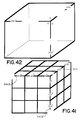
- Fig. 41 shows a coarsely discretized three dimensional configuration space.
- Fig. 42 shows a three dimensional configuration space.
- Fig. 43 is a flow chart of an alternate embodiment of the method of path planning.
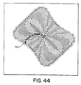
- Fig. 44 shows a configuration space budded according to the method of Fig. 43.
- a robot has degrees of freedom.
- the degrees of freedom are the independent parameters needed to specify its position in its task space. Some examples follow.
- a hinged door has 1 degree of freedom. In other words, any position can be characterized by one parameter, an opening angle.
- a robot which moves freely over a factory floor has two degrees of freedom, for instance the x- and y- position coordinates.
- An object in space can be considered to have six degrees of freedom.
- the 6 independent parameters that need to be specified are three position coordinates and three orientation angles. Therefore in order for a robot to be capable of manipulating an object into an arbitrary position and orientation in space, the robot must have at least six degrees of freedom.
- An example of a commercially available robot with six degrees of freedom is the Puma 562, manufactured by Unimation, Inc.
- a rotational degree of freedom is a degree of freedom that corresponds to an angle about a rotation axis of a robot joint.
- a rotational degree of freedom is a periodic parameter with values running from 0° to 360°; i.e. 360° corresponds to the same configuration of the robot as does 0°.
- Translational degrees of freedom correspond to non-periodic parameters that can take on values over an infinite range. Usually, however, the ranges of both rotational and translational degrees of freedom are limited by the scope of the robot.
- the “configuration space” of a robot is the space spanned by the parameters of the robot.
- the configuration space has one dimension for each degree of freedom of the robot.
- a point in configuration space will be called a "state”.
- Each "state" in an n-dimensional configuration space is characterized by a set of n values of the n robot degrees of freedom.
- a robot in the position characterized by the set of values is in a certain configuration.
- the set of states in the configuration space correspond to the set of all possible robot configurations.
- the configuration space is "discretized”. This means that only a limited number of states are used for calculations.
- Fig. 2 shows a data structure 1503 which is used as the configuration space of a robot with two degrees of freedom.
- Data structure 1503 is an MxN matrix of configuration states. The states are identified by their indices (i,j), where i represents a row number and j represents a column number.
- Each state (i,j) is itself a data structure as shown at 1501 and has a cost-to-goal field 1502 and a direction arrows field 1504. These fields are filled in by "budding” as described below.
- the cost-to-goal field 1502 generally contains a number which represents the cost of transition to get from the present state to a nearest "goal state”.
- "Goal states" represent potential end points of th e path to be planned.
- the cost of a transition on configuration space is a representation of a "criterion" or constraint in task space.
- a criterion is a cost according to which a user seeks to optimize. Examples of criteria that a user might chose are: amount of fuel, time, distance, wear and tear on robot parts, and danger.
- the direction-arrows field 1504 can contain zero or more arrows which indicate a direction of best transition in the configuration space from the present state to a neighbor state in the direction of the goal state resulting in a path of least total cost.
- Arrows are selected from sets of permissible transitions between neighboring states within the configuration space.
- the term "neighbor state” is used herein to mean a state which is reached from a given state by a single permissible transition.
- One set of arrows could be ⁇ up, down, right, left ⁇ , where, for instance, "up” would mean a transition to the state immediately above the present state.
- Another set of arrows could be ⁇ NORTH, SOUTH, EAST, WEST, NE, NW, SE, SW ⁇ .
- a third set of arrows could be ⁇ ( 0,1 ), ( 1,0 ), ( 0, -1 ), ( -1,0 ), ( 1,1 ), ( 1,-1 ), ( -1,1 ), ( -1,-1 ), ( 1,2 ), ( -1,2 ), ( 1,-2 ), ( -1,-1 ), ( 2,1 ), (-2,1), (2,-1), (-2, -1) ⁇ .
- the arrows "up”, “NORTH”, and "( -1,0 )" are all representations of the same transition within the configuration space. In general one skilled in the art may devise a number of sets of legal transitions according to the requirements of particular applications.
- any unambiguous symbolic representation of the set of permissible transitions can serve as the direction arrows.
- transition to a "neighbor" state in a two dimensional matrix 1503 actually requires a "knight's move", as that term is known from the game of chess.
- (1, -2) represents the move in the neighbor direction "down one and left 2".
- a metric In the configuration space, a metric is defined.
- the "metric" specifies for each state in configuration space the cost of a transition to any neighboring state.
- This metric may be specified by a function.
- a locally Euclidean metric can be defined as follows. As a state (i,j), the cost of a transition in a neighbor removed from (i,j) by directon arrow (di,dj) is given by di2 + dj2 . In other situations, it is more convenient to compute the metric in advance and store it. Obstacles can be represented in the metric by transitions of infinite cost. A transition between two arbitrary states must take the form of a series of transitions from neighbor to neighbor. The cost of any arbitrary path from a start state to a goal state is the sum of the costs of transitions from neighbor to neighbor along the path.
- a standard data structure called a heap is used to maintain an ordering of states. This is only one of many possible schemes for ordering, but the heap is considered to be the most efficient schedule for implementations with a small nubmer of parallel processors. Heaps are illustrated in Figs. 4b, 6, 8, 9, 10, 12 and 14.
- the heap is a balanced binary tree of nodes each representing a configuration state. In the preferred embodiment, the nodes actually store the indices of respective configuration states.
- each parent state e.g. at 601 has a lower cost-to-goal than either of its two children states e.g. at 602. Therefore, the state at the top of the heap, e.g. at 600, is that with the least value of cost-to-goal.
- Heaps are well known data structures, which are maintained using well known methods.
- One description of heaps and heap maintenance may be found in Aho et al., The Design and Analysis of Computer Algorithms , (Addison-WEsley 1974) pp 87-92.
- other ways of ordering states may be used during budding. For instance, a gueue can be used. This means that nodes are not necessarily budded in order of lower cost.
- Fig. 1a gives a general overview of steps used in generating a series of set points using the method of the invention.
- box 150 the configuration space is set up and permitted direction arrows are specified.
- One skilled in the art might devise a number of ways of doing this.
- the method is that of specifying aspects of the configuration space interactively.
- the number of states in a configuration space might be chosen to reflect how finely or coarsely a user wishes to plan a path.
- the set of direction arrows may be chosen to be more complete to get finer control of direction.
- the set of direction arrows may be chosen to be less complete if speed of path planning is more important than fine control of direction.
- a "background metric" is induced by a criterion.
- a background metric is one which applies throughout a configuration space without taking into account local variations which relate to a particular problem.
- Another option offered by the method is to specify the transition costs interactively.
- box 152 obstacles and constraints are transformed from task space to configuration space. This transformation generates obstacle states and/or constraint states. In addition or alternatively the transformation can represent obstacles and constraints as part of the metric. Boxes 151 and 152 are represented as separate steps in Fig. 1a, but in fact they can be combined.
- goals are transformed from points in task space to one or many goal states in configuration space.
- Budding results in filling the direction-arrows fields of the configuration space with direction arrows.
- a start state is identified.
- the start point in task space can be input by a user, or it can be sensed automatically, where applicable. This start point must then be transformed into a state in configuration space. If robot encoders are read, or the command WHERE in Val II is used one obtains the parameters of the start state immediately, without any need for transformations. The WHERE command returns the joint encoder angles in degrees.
- the method follows the direction arrows set up in box 154 from the start point indicated in box 155 to the goal state.
- the path states passed through in box 156 are sent to a robot at 157.
- the path can be sent in the form of set points.
- Each set point can then be a parameter of a MOVE POINT () command in Val II.
- the set points can be transformations into task space of the path states passed through in box 156.
- the set points can be the path states themselves. As will be discussed below, in some applications the set points need not be used to direct a robot. They can also be used as instructions to human beings.
- Fig. 1b expands box 154 of Fig. 1a.
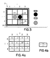
- Fig. 3 represents a factory floor 21 on which a robot is to travel.
- the map of the actual room is called a "task space".
- the floor consists of cells. There are four cells horizontally and three cells vertically. The robot moves from cell to cell, in any of 8 directions: horizontally, vertically, or diagonally.
- the factory floor is bounded by walls 24. There is a pillar 23 which is an obstacle to the movement of the robot.
- the floor sags.
- the sagging floor in cell 25 is a constraint to the movement of the robot.
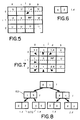
- Fig. 4a is a configuration space representation of the task space of Fig.3.
- Configuration space represents the combination of all the parameters of the task space. It is noted that the configuration space has twelve configuration states (0,0), (0,1), (0,2), (0,3), (1,0), (1,1), (1,2), (1,3), (2,0), (2,1), (2,2), and (2,3), described by the i and j locations on the factory floor and denoted as (i, j).
- Each configuration state has a cost-to-goal field 1502 and a direction-arrows field 1504, as shown in Fig.2.
- the set of arrows to be used in the direction arrows field 1504 are ⁇ ( 0,1 ), ( -1,1 ), ( -1,0 ), ( -1,-1 ), ( 0,-1 ), ( 1,-1 ), ( 1,0 ), (1,1 ) ⁇ (or ⁇ E, NE, N, NW, W, SW, S, SE) ⁇ , which correspond to the 8 directions in task space.
- moving from one state to a neighbor state in the configuration space of Fig. 4 corresponds to moving from cell to cell in the task space of Fig.3.
- Propagating cost waves is treating layer after layer of unprocessed states. If a queue is used to schedule budding, unprocessed states are treated first in, first out. If a heap is used, then the lowest cost node will always be budded first.
- 'time' is taken to be the cost criterion of movement. It is assumed that the horizontal or vertical movement from cell to cell in the task space generally takes one unit of time. A diagonal movement generally takes ⁇ 2 units of time, which can be rounded off to 1.4 units of time.
- transition cost of movement is not commutative (that is, there may be different costs for moving from (2,2) to (1,1) and from (1,1) to (2,2).
- the sagging floor 25 it takes longer to move out of the cell than into the cell.
- the cost into the sagging floor area 25 is taken to be the same as a normal movement. It is assumed for this simple problem that the robot slows down when moving uphill, but does not go faster downhill.
- the metric for transition costs between states of the configuration space is different from the cost criterion of movement in the task space, because cost waves are propagated from goal state to start state, in other words the transition costs are associated with transitions in configuration space.
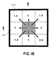
- the data structure of Fig.18 illustrates the value of the metric applicable to state (1,1) of the configuration space of Fig. 4a.
- a data structure is shown which illustrates the value of the metric applicable to state (1,1) of the configuration space of Fig.3.
- State (1,1) corresponds to the goal cell 22.
- a transition from state (1,1) to state (1,0) indicated at 1801 would take one unit of time and therefore has a cost of one.
- a transition from state (1,1) to state (0,0) indicated at 1802 has a cost of 1.4.
- a transition from state (1,1) to state (2,2) has a cost of 2.8, indicated at 1803. This transition cost indicates that climbing out of the sagging floor area 25 to the goal 22 costs 2.8 units of time.
- the transition cost of Fig. 18 represents the cost criterion of movement in the task space, in a direction opposite to the transition.
- Fig. 19 illustrates the values of the metric applicable to the entire configuration space of Fig. 4a.
- uncosted values U are assigned to the cost-to-goal field of each configuration state, and all the direction arrows fields are cleared.
- INF infinite values are set in the cost-to-goal field of configuration states (1,2) which represent obstacles such as the pillar 23. Since Fig. 4a is a highly simplified example, there is only one obstacle (1.2). In addition, the bounding walls 24 are obstacles. However, there are often many more obstacles in a real situation.
- Box 153 assigns zero O to the cost-to-goal fields of the configuration states which represent goals (1,1). Since Fig. 4a represents a highly simplified example, there is only one goal (1,1) shown. However, in a real world example there may be many goals. Also in box 153, the indices of the goals (1,1) are added to a heap. Standard methods of heap maintenance are employed for addition and removal of states to/from the heap. As a result, the state with the lowest cost will always be the top state of the heap. In the example of Fig. 4a, the sample goal has indices (1,1). Therefore, the indices (1,1) are added to the heap. In a more complicated example, with more goals, the indices of all the goals are added to the heap.
- Fig. 4a illustrates the configuration space after the completion of boxes 150, 151, 152, and 153 of Fig. 1a.
- Fig. 4b illustrates the corresponding heap.
- Box 14 of Fig. 1b checks to see if the heap is empty. In the example of Fig. 4b, the heap is not empty. It contains the indices (1,1) of the goal. Therefore the algorithm takes the NO branch 15 to box 16.
- Box 16 takes the smallest cost item from the heap (top state), using a standard heap deletion operation.
- the goal (1,1) is the current smallest cost item, with a cost of O.
- Neighbor states are those states which are immediately adjacent to the top state.
- the neighbor states at the present stage of processing are the states (0,0), (0,1), (0,2), (1,0), (1,2), (2,0), (2,1), and (2,2). So far, the neighboring states have not been checked. Therefore the method takes the NO branch 181 from box 17.
- the transition cost between the top state and its neighboring states is calculated using the metric function.
- transition cost between state (1,1) and state (0,2) is 1.4.
- Transition costs from state (1,1) to states (1,0), (2,0), (2,1), (2,2), (0,1), and (0,0) are calculated analogously, and are repsectively 1, 1.4, 1, 2.8, 1. 1.4.
- the transition from the top state (1,1) to the obstacle state (1,2) is INF. These are given here beforehand for convenience; but box 18 calculates each of these transition costs one at a time as part of the loop which includes boxes 17, 18, 19, 120, 121, 122, and 125.
- Box 19 compares the sum of the transition cost and the contents of the cost-to-goal field of the top state with the contents of the cost-to-goal field of the neighboring state.
- the transition cost is 1.4 and the contents of the cost-to-goal field of the top state are O.
- the sum of 1.4 and O is 1.4.
- the contents of the cost-to-goal field of the state (0,2) are currently U, uncosted, indicating that state (0,2) is in its initialized condition.
- One way to implement "U” is to assign to the cos-to-goal field a value which exceeds the largest possible value for the configuration space, other than INF. Performing the comparison in Box 19 thus gives a comparison result of " ⁇ ". Therefore the method takes branch 124 to box 121. Following branch 124 will be referred to herein as "improviding a state.
- box 121 the cost-to-goal field of the neighbor state is updated with the new (lower) cost-to-goal, i.e. the sum of the transition cost and the contents of the cost-to-goal field.
- the cost-to-goal field is updated to 1.4.
- box 121 adds an arrow pointing to the top state in the direction arrows field of the neighboring state. In the case of state (0,2), the arrow added is (1,-1).
- the downard direction on the figure corresponds to an increase in the first value of the direction arrow.
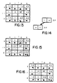
- the results of box 121 on state (0,2) are illustrated in Fig.5.
- box 122 which follows box 121, the indices (i,j) of the neighboring state (0,2) are added to the heap. This is illustrated in Fig.6. The cost values are noted next to the state indices, for reference, but are not actually stored in the heap.
- the method now returns control to box 17. This return results in a loop.
- the method executes boxes 17, 18, 19, 121, and 122 for each of the neighboring states, other than the obstacle. For the obstacle, the method takes branch 126 to box 125. Since the transition cost is infinite, branch 127 is taken from box 125 to return control to box 17.
- the effects on the configuration states which are neighbors of the goal (1,1) are illustrated in Fig.7.
- the heap corresponding to Fig.7 is illustrated at Fig.8.
- next top state is retrieved. This is the smallest cost item which is on top of the heap.
- the next top state has indices (0,1), 600 in Fig.8.
- the (0,1) state at the top of the heap is the next to be "budded".
- the neighbors in the directions (-1,1), (-1,0), and (-1,-1) have an infinite transition cost since the walls are constraints. No impact can be made on any other neighbor of the (0,1) state, so no changes are made to the configuration space.
- the cost-to-goal field of (0,2) is already set to 1.4.
- the transition cost to state (0,2) is 1.
- the sum of the transition cost and the top state's (0,1)'s cost-to-goal is 2. The sum is thus greater than the neighbor's (0,2)'s pre-existing cost-to-goal. Therefore branch 124 is not taken. No improvement can be made.
- Branch 129 is taken instead, returning control to box 17. Taking branch 129 is referred to herein as "not impacting" another state.
- the budding of (0,1) is complete.
- the heap now is as shown in Fig.9.
- the top state (1,0) from Fig. 9 is the next to be budded. Budding of this state does not result in any impact, nor does the budding of node (2,1) (the next to be budded after (1,0)). After consideration of state (2,1) the heap appears as shown in Fig. 10.
- Budding of (2,2) results in improvement of the "uncosted" state (2,3) to its right, so we add the new cost and arrow to that neighbor, and add (2,3) to the heap. No impact can be made on any other neighbor.
- the results are illustrated in Figs. 13 and 14.
- direction arrows field can contain more than one arrow as illustrated in 1504 of Fig. 2.
- the last node in the heap to be budded is (2,3) the budding of which does not impact on any neighbors.
- a path can be followed from any starting position to the goal by simply following the direction-arrows values.
- the cost in each configuration state gives the total cost required to reach the goal from that state. If the user wanted to start at (2,3), 2 alternate routes exist. Both cost 3.8 (units of time). These routes are illustrated in Figs. 15 and 16. In Fig. 15 the route starts at (2,3) and proceeds to (1,3), (0,2), and finally to the goal state (1,1) in that order. In Fig. 16 the route goes over the sagging floor from (2,3) to (2,2) and then to the goal state (1,1). The series of set points sent to the robot would thus be (2,3), (1,3), (0,2), (1,1), or (2,3) (2,2), (1,1). Both will lead to arrival of the robot in 3.8 units of time.
- Appendix A contains source code implementing the method of Figures 1a and 1b.
- Fig. 17 represents a two-link robot.
- the robot has a shoulder joint 1601, an upper arm 1602, an elbow joint 1603, forearm 1604, a protruding part 1610 beyond the elbow joint 1603, and an end effector 1605. Because the two-link robot has two joints, the elbow joint 1603 and the shoulder joint 1601, the robot has two rotational degrees of freedom.
- Fig. 17 illustrates a convention for measuring the angles of rotation.
- the angle 1606 of the shoulder joint 1601 is 60°, measured from a horizontal axis 1607.
- the angle 1608 of the elbow 1603 is 120°, measured from a horizontal axis 1609.
- Fig. 20 represents a coarse discrete configuration space of the robot of Fig. 17. This coarse configuration space is presented as a simplfified example. In practice, one skilled in the art would generally use a finer configuration space to allow for finer specification of the motion of the corresponding robot arm.
- the first degree of freedom in Fig. 20 is the angle of the shoulder joint of the robot arm. This first degree of freedom is plotted along the vertical axis of Fig. 20.
- the second degree of freedom is the angle of elbow of the robot arm and is plotted along the horizontal axis.
- the discretization of the angles is in multiples of 60°.
- the position of the robot which corresponds to each state of the configuration space is illustrated within the appropriate box in Fig. 20.
- the state (0°,0°) corresponds to the position in which the arm is competely extended horizontally, with both the shoulder and the elbow at 0°.
- the fat part of the arm, e.g. 2001 is the upper arm, between the shoulder and the elbow.
- the thin part of the arm, e.g. 2002, is the forearm, between the elbow and the end effector.
- each state of the configuration space of Fig.20 has a cost-to-goal and a direction arrows field. These fields are not shown again in Fig. 20.
- Fig. 21 is a fine-grained configuration space for a two-joint robot arm.
- the fine-grained configuration space is a 64x64 array.
- the individual states of the fine-grained configuration space are not demarcated with separator lines, unlike Fig. 20, because the scale of the figure is too small to permit such separator lines.
- the vertical axis is the angle of the elbow.
- the angle of the elbow increases from top to bottom from 0° to 360°.
- the horizontal axis is the angle of the shoulder.
- the angle of the shoulder increases from left to right from 0° to 360°.
- the axes were marked off in units of 60°. However, in the fine space of Fig. 21, the axes are divided into units of 360°/64, or approximately 5.6°.
- Fig. 22 is a task space which corresponds to the configuration space of Fig. 21.
- the upper arm of the two-link robot is at 2201.
- the forearm is at 2202.
- a goal is shown at 2203.
- An obstacle is shown at 2204.
- the robot is shown in a position which it in fact cannot assume, that is overlapping an obstacle. This position has been chosen to illustrate a point in the configuration space.
- the white state 2101 of the configuration space in Fig. 21 corresponds to the position of the robot in the task space of Fig. 22.
- the white state 2101 is located in a black region 2102 which is a representation of the obstacle 2204.
- the black areas represent all of the configurations in which the robot will overlap the obstacle.
- the goal appears at 2104.
- One skilled in the art might devise a number of ways of determining which regions in configuration space correspond to an obstacle in task space.
- One simple way of making this determination is to simulate each state of the configuration space one by one in task space and test whether each state corresponds to the robot hitting the obstacle.
- Standard solid-modelling algorithms may be used to determine whether the robot hits the obstacle in task space.
- One such set of algorithms is implemented by representing surfaces using the B-rep technique in the Silma package sold by SILMA, 211 Grant Road, Los Altos, CA 94022.
- the forearm 2202 hits the obstacle 2204, which corresponds to the white state 2101 of the configuration space.
- the white state 2101 therefore becomes part of the obstacle region.
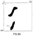
- Figs. 23 and 24 illustrate the determination of an additional state in the obstacle region of the configuration space.
- the elbow 2301 hits the obstacle 2302. This position of the robot corresponds to the white state 2401 in Fig. 24.
- the states should be assigned a cost-to-goal of INF as indicated in box 12 of Fig. 1b.
- assigning a cost-to-goal of INF will be represented by making the region of states corresponding to the obstacle black in the configuration space.
- Figs. 28, 29 and 30 illustrate various states in the process of budding for such a space, once the obstacle regions and goal states have been located.
- a metric data structure such as is illustrated in Fig. 19 may become awkward.
- a function can be used in place of the data structure.
- the configuration space of Fig. 28 corresponds to the task space of Fig. 27.
- the obstacle regions 2801 corespond to the obstacle 2701.
- the goal 2703 corresponds to the state at 2802.
- the states at 2803 and 2804 both correspond to the goal 2702. This occurs because the robot arm can take two positions and still have the end effector at the same point. In one of these two positions, the robot looks like a right arm and in the other position the robot looks like a left arm. In Fig. 28, the process of budding around the goal states has begun. A number of direction arrows, e.g. at 2805, appear. It is to be noted that the configuration space of Fig. 28 corresponds to two rotational degrees of freedom and is therefore periodic so that the picture will 'wrap-around' both horizontally and vertically.
- Fig. 28 This manifests itself in that the configuration space of Fig. 28 is topologically equivalent to a torus. Therefore direction arrows, e.g. at 2806, which point to goal state 2802 appear instead to point to the boundaries of the configuration state. In fact, it is perfectly possible for a path of the robot to wrap around the configuration space.
- the configuration space of Fig. 30 shows how the direction arrows look when budding has been completed.
- Fig. 31 is the same as the task space of Fig. 27, except that the motion of the robot along a path from starting point 3101 to goal 2702 is shown.
- the motion is shown by the superposition of a number of images of the robot in various intermediate positions, e.g. 3102 and 3103, along the path.
- the path also appears on the configuration space of Fig. 30.
- the path appears as shaded dots, e.g. 3003 and 3304, which are not part of the obstacle region.
- the metric of Eq.(1) is a locally "Euclidean metric", because it allocates transition costs to the neighbor states equal to their Euclidean distance in configuration space.
- the path in configuration space in the absence of obstacle regions is an approximation of a straight line.
- the approximation is better if more directions are available as direction arrows.
- the accuracy of the approximation using the 8 direction arrows corresponding to the horizontal, vertical and diagonal transitions is about 5% maximum error, 3% average error.
- the accuracy of the approximation also using the knight's moves is about 1%.
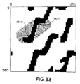
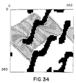
- Fig. 33 and Fig. 34 show two intermediate stages in budding.
- Fig. 35 shows the final result.
- the path found in configuration space is indicated by shaded states 35001. Note that the path is a curve in configuration space.
- Fig. 36 shows the path 36001 of the end effector in task space, and the the goal pose reached. Note that 36001 is almost a straight path.
- the smaller deviations from a straight path are due to the resolution in configuration space and obstacle avoidance. With angle increments of 5.6 degrees one cannot produce points along perfect straight lines.
- the larger deviations from a straight path are due to the fact that the robot should not only produce the shortest path for the end effector, but also avoid the obstacles.
- Fig. 37 shows all intermediate states of the robot as it moves from start to goal. This simultaneous optimization of collision-free paths with a minimization criterion is an important feature of the method.
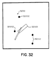
- Fig. 38 shows the configuration space corresponding to the same task space as Fig. 32, but using the metric of Eq.(1).
- Fig. 39 shows the path 39001 found using the configuration space of Fig. 38.
- a path minimizing time can also be planned for a robot in its configuration space, if the speed with which the robot moves in a particular configurion is known. The time the robot takes to make a transition from state (i,j) in the direction ( di,dj ) can be used as the cost for that transition. The minimal cost paths found by the method are then minimum time paths.
- Task dependent constraints can also be accommodated. For example, in carrying a cup containing a liquid, it is important that the cup not be tilted too much. In the configuration space, the states corresponding to a configuration of too much tilt can be made into obstacle regions. They do not correspond to physical obstacles in task space, but to constraints dependent on the task. The transition costs are progressively increased according to their proximity to obstacles regions imposed by the constraints. Such transition costs lead to a tendency to keep the cup upright. This metric will allow the robot to deviate slightly from an upright position, if this is needed for obstacle avoidance, with a tendency to return to the upright position.
- Fig. 40 illustrates a three-link robot with three rotational degrees of freedom.
- the robot has a waist 3201, shoulder 3203, an upper arm 3219, a forearm 3204, en elbow 3205, and an end effector 3207.
- Fig. 40 also illustrates the waist angle 3208, the shoulder angle 3209, and the elbow angle 3210.
- Fig. 41 illustrates a coarse three-dimensional configuration space corresponding to three rotational degrees of freedom.
- This configuration space corresponds to the robot of Fig. 40; however it could equally well be used for any robot with three rotational degrees of freedom.
- the configuration space has three axes: angle of waist 3401, angle of elbow 3402, and angle of shoulder 3403. The axes are divided into units of 120°.
- the coarse configuration space has 27 states (0°,0°,0°), (0°,0°,120°), (0°,0°,120°), (0°,0°,120°),
- Fig. 42 illustrates a fine configuration space. Here the demarcations between states are too small to fit in the scale of the figure.
- each state has a cost-go-goal field and a direction-arrows field; the principle difference being that the set of permissible directions of travel, direction arrows, is different in three dimensions from two dimensions.
- One set of possible direction arrows is ⁇ ( 0,0,1 ), ( 0,0,-1 ), ( 0,1,0 ), ( 0,-1,0 ), ( 1,0,0 ), ( -1,0,0 ) ⁇ ⁇ (right), (left), (up), (down), (forward), (backward) ⁇ which would allow for no diagonal motion.
- These direction arrows may be characterized as being parallel to the axes of the configuration space.
- Another set of direction arrows would be ⁇ ( 0,0,1 ), ( 0,0,-1 ), ( 0,1,0 ), ( 0,-1,0 , ( 1,0,0 ), ( -1,0,0 ), ( 0,1,1 ), ( 0,-1,1 ), ( 1,0,1 ), ( -1,0,1 ), ( 0,1,-1 ), ( 0,-1,-1 ), ( 1,0,-1 ), ( -1,0,-1 ) ( 1,1,0 ), ( -1,1,0 ), ( 1,-1,0 ), ( -1,-1,0 ), ( 1,1,1 ), ( 1,1,-1 ), ( 1,-1,1 ), ( -1,1,1 ) ( 1,-1,-1 ), ( -1,-1,1 ), ( -1,1,-1 ), ( -1,-1,-1 ) ⁇ .
- robots are not the only objects which can be directed using the method of Fig. 1b.
- the configuration space of Fig. 2 might equally well apply to a task space which is a city street map.
- the method of Fig. 1b could then be employed to plot the path of an emergency vehicle through the streets.
- a metric for this application should reflect the time necessary to travel from one point to another.
- One-way streets would have a certain time-cost for one direction and infinite cost in the illegal direction.
- Highways would generally have a lower time-cost than small side streets. Since highway blockages due to accidents, bad weather, or automobile failure are commonly reported by radio (broadcast and police) at rush hour, this information might be used as an input to increase expected time-costs on those constricted routes. This would result in the generation of alternate routes by the path planner.
- Figs. 1a and 1b could also be employed with the city street task space to generate electronic maps for automobiles.
- Dynamic emergency exit routes can be obtained for buildings that report the location of fire or other emergency.
- the currently used fixed routes for emergency exits can lead directly to a fire.
- a dynamic alarm system can report the suspected fire locations directly to a path planning device according to the invention.
- the path planning device can then light up safe directions for escape routes that lead away from the fire.
- the safest escape route may be longer, but away from the fire.
- 'safety' is the criterion.
- the method of the present invention finds a discrete approximation to the set of all geodesics perpendicular to a set of goal points in a space variant metric. "Following the direction arrows" is analogous to following the intrinsic gradient. Following the direction arrows from a specific start state yields the geodesic connecting the start state to the closest goal state. A device incorporating this method could be applied to the solution of any problem which requires the finding of such a geodesic.
- the early path detection feature makes use of the fact that as soon as the cost waves have been propagated just behond the starting state, the optimal path can be reported, since no further budding changes will affect the region between the start and goal.
- Fig. 43 shows the additional steps necessary for early path reporting.
- Fig. 43 is the same as Fig. 1b, except that several steps have been added.
- the method tests whether the value of the cost-to-goal field of the state at the top of the heap is greater than the cost-to-goal field of the start state. If the result of the test of box 3701 is negative, budding continues as usual, along branch 3702. If the result of the test of box 3701 is positive, the method follows branch 3703 to box 3704 where the path is reported. After the path is reported at box 3704, normal budding continues. It is possible to stop after this early detection if the entire cost field is not needed.
- Fig. 44 shows an example of configuration space in which the path 3701 has been reported prior to the 'normal' termination of budding.
- Another efficiency technique is to begin budding from both the goal and the start states. The path then is found when the expanding cost waves meet. Usually, a different metric must be used for budding the start state from that which is used for budding the goal states. This results from the fact that budding out from the start state would be in the actual direction of motion in the task space which is essentialy calling the same metric function with the top and neighbor states swapped. By contrast, budding from the goal states is in a direction opposite to motion in the task space.
- Fig. 1A 150 set up configuration space data structure and specify permitted direction arrows; 151 induce "background metric" depending on criterion; 152 transform obstacles and/or constraints from task space to configuration space; 153 transform goals; 154 bud; 155 identify start state; 156 follow direction arrows; 157 send set points to robot to perform movement.
- Fig. 1B 14 heap empty?; 16 take smallest cost item (top state) from heap; 17 Checked all neighbor states?; 18 Calculate transition cost (from metric function) between top & neighboring state; 19 Compare (transition cost + top state's cost-to-goal) to (neighbor state's cost-to-goal); 125 Transition Cost is INF (infinite)?; 120 Add a direction arrow (pointing to top state) to the neighbor state's direction arrows; 121 Update neighbor state with new (lower) cost-to-goal. Make neighbor's direction arrows point to top state; 122 Add neighbor's (i, j) location to heap.
- Fig. 43 3705 Start of Budding; 3706 Budding is complete; 3707 Heap empty? 3708 Take smallest cost item (top state) from heap; 3701 Top's cost-to-goal > Start's cost-to-goal?; 3704 Report Path; 3709 Checked all neighbor states?; 3710 Calculate transition cost (from metric function) between top & neighboring state; 3711 Compare (transition cost + top state's cost-to-goal) to (neighbor states's cost-to-goal); 3712 Transition Cost is INF (infinite)?; 3713 Add a direction arrow (pointing to top state) to the neighbor state's direction arrows; 3714 Update neighbor state with new (lower) cost-to-goal. Make neighbor's direction arrows point to top state; 3715 Add neighbor's (i, j) location to heap.
Landscapes
- Engineering & Computer Science (AREA)
- Physics & Mathematics (AREA)
- General Physics & Mathematics (AREA)
- Automation & Control Theory (AREA)
- Aviation & Aerospace Engineering (AREA)
- Geometry (AREA)
- Radar, Positioning & Navigation (AREA)
- Remote Sensing (AREA)
- Theoretical Computer Science (AREA)
- Robotics (AREA)
- Manufacturing & Machinery (AREA)
- Human Computer Interaction (AREA)
- Mechanical Engineering (AREA)
- Mathematical Optimization (AREA)
- Computer Networks & Wireless Communication (AREA)
- Evolutionary Computation (AREA)
- Computer Hardware Design (AREA)
- Pure & Applied Mathematics (AREA)
- Mathematical Analysis (AREA)
- Computational Mathematics (AREA)
- General Engineering & Computer Science (AREA)
- Computer Vision & Pattern Recognition (AREA)
- Multimedia (AREA)
- Electromagnetism (AREA)
- Manipulator (AREA)
- Control Of Position, Course, Altitude, Or Attitude Of Moving Bodies (AREA)
- Feedback Control In General (AREA)
- Numerical Control (AREA)
Claims (22)
- Procédé de commande d'un objet pour l'amener à suivre une route dans un espace de tâches entre un point de départ et un point de destination, ledit espace de tâches étant une représentation de l'espace tridimensionnel réel dans lequel ladite route est définie, ledit procédé comprenant les étapes consistant à :a. initialiser un espace de configuration qui correspond à l'espace de tâches, l'espace de configuration comprenant une pluralité d'états, chaque état ayant une dimension pour chaque degré de liberté de l'objet, lesdits états correspondant respectivement à un sous-ensemble discrétisé de toutes les positions de l'objet dans l'espace de tâches;b. transformer une première fois le point de destination en au moins un état de destination de l'espace de configuration;c. au départ de l'état de destination, affecter des valeurs de coût et de flèches directionnelles à des états voisins de l'espace de configuration, de telle sorte que chaque état voisin respectif qui peut être atteint se voie affecté d'une valeur de coût selon une métrique prédéfinie qui représente le coût d'une transition optimale de l'état voisin respectif à l'état de destination, et de telle sorte que chaque état voisin respectif se voie affecté d'au moins une valeur de flèche directionnelle qui représente une direction de déplacement le long de la transition de coût minimum;d. répéter l'étape c jusqu'à ce que tous les états pouvant être atteints de l'espace de configuration aient été traités;e. transformer une deuxième fois le point de départ en un état de départ;f. suivre les flèches directionnelles de l'état de départ vers l'état de destination pour obtenir une série de transitions dans l'espace de configuration qui constituent une représentation de la route dans ledit espace de tâches;g. fournir des points sur la route, de telle sorte que l'objet soit commandé pour suivre la route.
- Procédé selon la revendication 1, comprenant les étapes consistant à :a. déterminer, après l'étape de la deuxième transformation, si la route existe, une routeexistant lorsqu'il y a au moins une valeur de flèche directionnelle pour l'état de départ, etb. arrêter la planification de la route après l'étape de détermination, lorsqu'aucune route n'existe.
- Procédé selon la revendication 1, dans lequel l'étape d'initialisation consiste à choisir une valeur qui est une représentation grossière de l'espace de configuration.
- Procédé selon la revendication 1, comprenant l'étape consistant à choisir de manière interactive un ensemble de flèches directionnelles possibles.
- Procédé selon la revendication 1, dans lequel l'étape d'affectation consiste à choisir des valeurs des fèches directionnelles dans un ensemble comprenant des flèches directionnelles représentant des transitions parallèles aux axes de l'espace de configuration.
- Procédé selon la revendication 1, dans lequel l'étape d'affectation consiste à choisir des valeurs des flèches directionnelles dans un ensemble comprenant des flèches directionnelles représentant des transitions entre un premier état et des états respectifs d'une pluralité de deuxièmes états, lesdits deuxièmes états étant les états visibles d'un cube n de p états sur un côté, le cube n entourant le premier état, où n est un nombre entier positif représentant un certain nombre de degrés de liberté de l'objet et p est un nombre entier positif.
- Procédé selon la revendication 1, dans lequel l'étape d'affectation comprend la mesure des valeurs de transition de coût entre les états voisins par une métrique.
- Procédé selon la revendication 7, comprenant l'étape consistant à induire la métrique dérivée d'un critère.
- Procédé selon la revendication 8, comprenant l'étape consistant à utiliser le critère de réduction au minimum du temps de mouvement dans l'espace de tâches.
- Procédé selon la revendication 1, dans lequel l'objet est un robot avec des articulations mobiles et comprenant l'étape consistait à utiliser le critère de réduction au minimum du mouvement des articulations du robot.
- Procédé selon la revendication 8, comprenant l'étape consistant à utiliser le critère de réduction au minimum de la distance de mouvement dans l'espace de tâches.
- Procédé selon la revendication 1, dans lequel l'étape d'affectation comprend l'étape de greffage de chaque état, qui comprend les étapes consistant à :a. partir de l'état de destination;b. explorer les états voisins d'un état présent pour contrôler s'il n'y aucun besoin de heurt;c. heurter l'état voisin approprié, ce qui comprend les étapes consistant à :i. améliorer les états voisins qui ont une valeur de coût supérieure à ce qui est nécessaire en mettant à jour les valeurs de coût et les valeurs de flèches directionnelles, etii. établir des routes équivalentes en ajoutant des valeurs de flèches directionnelles;d. passer à un état supérieur suivant, qui est choisi parce qu'il a une valeur de coût suivant immédiatement moindre pour atteindre l'état de destination, ete. revenir à l'étape b jusqu'à ce que tous les états aient été explorés.
- Procédé selon la revendication 12, dans lequel l'étape d'affectation comprend l'évaluation du coût selon une métrique variable dans l'espace.
- Procédé selon la revendication 12, dans lequel l'étape d'affectation comprend l'évaluation du coût selon une métrique variable dans l'espace, dans laquelle des points de limitation de l'espace de tâches sont exprimés comme nécessitant des transitions de coût supérieures dans l'espace de configuration.
- Procédé selon la revendication 1, comprenant une autre étape consistant à effectuer une troisième transformation d'au moins un autre point de destination en d'autres états de destination correspondants dans l'espace de configuration, dans lequel l'étape d'affectation comprend l'affectation de valeurs de coût et de valeurs de flèches directionnelles qui représentent le coût et la direction d'une route de transition optimale depuis l'état respectif et jusqu'à un état de coût moindre parmi les états de destination, et dans lequel l'étape suivante consiste à suivre les flèches de direction depuis l'état de départ jusqu'à l'état de coût moindre parmi les états de destination.
- Procédé selon la revendication 1, comprenant l'étape consistant à effectuer une troisième transformation d'au moins un point d'obstacle de l'espace de tâches en un état d'obstacle de l'espace de configuration; et dans lequel l'étape d'affectation comprend l'affectation de coût et de flèches directionnelles, de telle sorte que la route de transition optimum évite l'état d'obstacle et ainsi que l'état d'obstacle n'ait aucune valeur de flèche directionnelle; I'étape suivante permettant d'obtenir une route qui évite l'obstacle.
- Procédé selon la revendication 16, dans lequel la troisième étape de transformation comprend l'affectation d'une valeur de coût sensiblement infini à l'état d'obstacle, I'état d'obstacle devenant ainsi partie d'une métrique variable dans l'espace qui mesure le coût.
- Appareil de commande d'un objet pour lui faire suivre une route à travers un espace de tâches donné entre un point de départ et un point de destination, la route satisfaisant à un critère de coût donné, ledit espace de tâches étant une représentation de l'espace tridimensionnel réel où ladite route est définie, l'appareil comprenant :a. une mémoire pour stocker un espace de configuration discrétisé qui comprend une pluralité d'états dont chacun a une dimension pour chaque degré de liberté de l'objet, lesdits états correspondant à un sous-ensemble discrétisé de toutes les positions de l'objet dans l'espace de tâches, les états étant agencés, de telle sorte que chaque état ait une pluralité d'états voisins situés le long de directions de transition admissibles respectives;b. des moyens pour initialiser les états;c. des moyens pour stocker des informations de destination correspondant au point de destination dans un état de destination respectif;d. des moyens pour mesurer le coût de transition de chaque état vers ses états voisins le long des directions admissibles selon une métrique prédéterminée variable dans l'espace;e. des moyens pour propager les oncles de coût depuis l'état de destination en utilisant les moyens de mesure, les moyens de propagation affectant à chaque état adjacent une valeur de coût et une direction de déplacement correspondant à une transition de moindre coût à partir de l'état du point de destination; lesdits moyens exécutant, en outre, la propagation des ondes de coût jusqu'à ce que tous les états pouvant être atteints dans l'espace de configuration aient été atteints;f. des moyens pour déterminer une série de transitions d'états discrètes, les moyens de détermination correspondant à ladite route, les moyens de détermination déterminant ladite série d'états en partant du point de départ et en suivant les valeurs de coûts et de directions de déplacement affectées à l'état de départ et aux états suivants, constituant ainsi une représentation de ladite route.
- Appareil selon la revendication 18, dans lequel :a. l'objet est un robot, etb. les états discrets le long de la route de transition correspondent à des points de consigne du robot.
- Appareil selon la revendication 18, dans lequel :a. l'objet est un véhicule de secours;b. les états discrets le long de la route de transition correspondent à des emplacements de rues vers lesquels le véhicule de secours doit se diriger, etc. l'appareil comprend des moyens pour transmettre les états discrets au chauffeur du véhicule de secours.
- Appareil selon la revendication 18, dans lequel :a. l'objet est un système d'alarme d'urgence dans un bâtiment;b. l'objet est une personne essayant de s'échapper du bâtiment;c. la route représente la voie la plus sûre dans une situation d'urgence, etd. l'appareil comprend des moyens pour communiquer la route à la personne concernée.
- Appareil selon la revendication 18, dans lequel :a. l'appareil est une carte électronique;b. l'objet est une personne essayant de trouver une route dans une zone nouvelle, etc. les états discrets correspondent à des emplacements de rues vers lesquels la personne doit se diriger.
Applications Claiming Priority (2)
| Application Number | Priority Date | Filing Date | Title |
|---|---|---|---|
| US12350287A | 1987-11-20 | 1987-11-20 | |
| US123502 | 1987-11-20 |
Publications (3)
| Publication Number | Publication Date |
|---|---|
| EP0317020A2 EP0317020A2 (fr) | 1989-05-24 |
| EP0317020A3 EP0317020A3 (en) | 1989-10-25 |
| EP0317020B1 true EP0317020B1 (fr) | 1995-04-19 |
Family
ID=22409048
Family Applications (1)
| Application Number | Title | Priority Date | Filing Date |
|---|---|---|---|
| EP88202551A Expired - Lifetime EP0317020B1 (fr) | 1987-11-20 | 1988-11-15 | Méthode et dispositif pour l'établissement de route |
Country Status (5)
| Country | Link |
|---|---|
| US (1) | US6604005B1 (fr) |
| EP (1) | EP0317020B1 (fr) |
| JP (1) | JP2840608B2 (fr) |
| KR (1) | KR0133294B1 (fr) |
| DE (1) | DE3853616T2 (fr) |
Cited By (2)
| Publication number | Priority date | Publication date | Assignee | Title |
|---|---|---|---|---|
| US20090182464A1 (en) * | 2008-01-11 | 2009-07-16 | Samsung Electronics Co., Ltd. | Method and apparatus for planning path of mobile robot |
| US8417491B2 (en) | 2005-10-11 | 2013-04-09 | Koninklijke Philips Electronics N.V. | 3D tool path planning, simulation and control system |
Families Citing this family (47)
| Publication number | Priority date | Publication date | Assignee | Title |
|---|---|---|---|---|
| US5187667A (en) * | 1991-06-12 | 1993-02-16 | Hughes Simulation Systems, Inc. | Tactical route planning method for use in simulated tactical engagements |
| EP0546633A2 (fr) * | 1991-12-11 | 1993-06-16 | Koninklijke Philips Electronics N.V. | Préparation de la voie dans un environnement indéterminé |
| EP0609928B1 (fr) * | 1993-01-22 | 2000-08-23 | Koninklijke Philips Electronics N.V. | Méthode et appareil pour identifier et contrôler un déplacement vers un rendez-vous |
| JPH07186074A (ja) * | 1993-12-27 | 1995-07-25 | Agency Of Ind Science & Technol | ロボット制御装置 |
| US6226622B1 (en) * | 1995-11-27 | 2001-05-01 | Alan James Dabbiere | Methods and devices utilizing a GPS tracking system |
| US6909746B2 (en) * | 2001-03-30 | 2005-06-21 | Koninklijke Philips Electronics N.V. | Fast robust data compression method and system |
| EP1587650B1 (fr) * | 2003-01-31 | 2018-08-29 | Thermo CRS Ltd. | Procédé de prévision de mouvement inférentiel syntactique destiné à des systèmes robotisés |
| US7216033B2 (en) | 2003-03-31 | 2007-05-08 | Deere & Company | Path planner and method for planning a contour path of a vehicle |
| US7079943B2 (en) * | 2003-10-07 | 2006-07-18 | Deere & Company | Point-to-point path planning |
| US7110881B2 (en) * | 2003-10-07 | 2006-09-19 | Deere & Company | Modular path planner |
| US8352174B2 (en) | 2004-01-15 | 2013-01-08 | Algotec Systems Ltd. | Targeted marching |
| US7440447B2 (en) * | 2004-03-25 | 2008-10-21 | Aiseek Ltd. | Techniques for path finding and terrain analysis |
| US20100235608A1 (en) * | 2004-03-25 | 2010-09-16 | Aiseek Ltd. | Method and apparatus for game physics concurrent computations |
| US7512485B2 (en) * | 2005-03-29 | 2009-03-31 | International Business Machines Corporation | Method for routing multiple paths through polygonal obstacles |
| DE102006007623B4 (de) * | 2006-02-18 | 2015-06-25 | Kuka Laboratories Gmbh | Roboter mit einer Steuereinheit zum Steuern einer Bewegung zwischen einer Anfangspose und einer Endpose |
| FR2900360B1 (fr) * | 2006-04-28 | 2008-06-20 | Staubli Faverges Sca | Procede et dispositif de reglage de parametres de fonctionnement d'un robot, programme et support d'enregistrement pour ce procede |
| US7912574B2 (en) | 2006-06-19 | 2011-03-22 | Kiva Systems, Inc. | System and method for transporting inventory items |
| US8538692B2 (en) | 2006-06-19 | 2013-09-17 | Amazon Technologies, Inc. | System and method for generating a path for a mobile drive unit |
| US20130302132A1 (en) | 2012-05-14 | 2013-11-14 | Kiva Systems, Inc. | System and Method for Maneuvering a Mobile Drive Unit |
| US7920962B2 (en) | 2006-06-19 | 2011-04-05 | Kiva Systems, Inc. | System and method for coordinating movement of mobile drive units |
| US8220710B2 (en) | 2006-06-19 | 2012-07-17 | Kiva Systems, Inc. | System and method for positioning a mobile drive unit |
| EP2005886B1 (fr) * | 2007-06-19 | 2011-09-14 | Biocompatibles UK Limited | Procédé et appareil de mesure de la texture de la peau |
| KR100956663B1 (ko) * | 2007-09-20 | 2010-05-10 | 한국과학기술연구원 | 로봇의 경로 설계 방법 및 그 로봇 |
| JP4978494B2 (ja) * | 2008-02-07 | 2012-07-18 | トヨタ自動車株式会社 | 自律移動体、及びその制御方法 |
| US9946979B2 (en) * | 2008-06-26 | 2018-04-17 | Koninklijke Philips N.V. | Method and system for fast precise path planning |
| RU2012122469A (ru) | 2009-11-06 | 2013-12-20 | Эволюшн Роботикс, Инк. | Способы и системы для полного охвата поверхности автономным роботом |
| EP2506106B1 (fr) | 2009-11-27 | 2019-03-20 | Toyota Jidosha Kabushiki Kaisha | Objet mobile autonome et procédé de contrôle |
| EP2546712A1 (fr) * | 2011-07-12 | 2013-01-16 | Siemens Aktiengesellschaft | Procédé de fonctionnement d'une machine de production |
| US9046888B2 (en) * | 2012-06-27 | 2015-06-02 | Mitsubishi Electric Research Laboratories, Inc. | Method and system for detouring around features cut from sheet materials with a laser cutter according to a pattern |
| US11370128B2 (en) | 2015-09-01 | 2022-06-28 | Berkshire Grey Operating Company, Inc. | Systems and methods for providing dynamic robotic control systems |
| ES2845683T3 (es) | 2015-09-01 | 2021-07-27 | Berkshire Grey Inc | Sistemas y métodos para proporcionar sistemas de control robótico dinámico |
| EP3355824A1 (fr) * | 2015-09-29 | 2018-08-08 | Koninklijke Philips N.V. | Dispositif de commande d'instrument pour chirurgie mini-invasive assistée par robot |
| US10625432B2 (en) | 2015-11-13 | 2020-04-21 | Berkshire Grey, Inc. | Processing systems and methods for providing processing of a variety of objects |
| US9740207B2 (en) * | 2015-12-23 | 2017-08-22 | Intel Corporation | Navigating semi-autonomous mobile robots |
| US10350755B2 (en) | 2016-02-08 | 2019-07-16 | Berkshire Grey, Inc. | Systems and methods for providing processing of a variety of objects employing motion planning |
| WO2017139613A1 (fr) * | 2016-02-11 | 2017-08-17 | Massachusetts Institute Of Technology | Planification de mouvement pour systèmes robotiques |
| JP6154509B2 (ja) * | 2016-04-04 | 2017-06-28 | 富士機械製造株式会社 | ワーク搬送装置 |
| JP6931457B2 (ja) * | 2017-07-14 | 2021-09-08 | オムロン株式会社 | モーション生成方法、モーション生成装置、システム及びコンピュータプログラム |
| CN113396035A (zh) | 2019-02-27 | 2021-09-14 | 伯克希尔格雷股份有限公司 | 用于在可编程运动系统中的软管布线的系统和方法 |
| CN110045731B (zh) * | 2019-03-26 | 2022-04-12 | 深圳市中科晟达互联智能科技有限公司 | 一种路径规划方法、电子装置及计算机可读存储介质 |
| US11254003B1 (en) | 2019-04-18 | 2022-02-22 | Intrinsic Innovation Llc | Enhanced robot path planning |
| ES2982678T3 (es) | 2019-04-25 | 2024-10-17 | Berkshire Grey Operating Company Inc | Sistema y método para mantener la vida útil de una manguera de vacío en sistemas de enrutamiento de mangueras en sistemas de movimientos programables |
| US11504849B2 (en) * | 2019-11-22 | 2022-11-22 | Edda Technology, Inc. | Deterministic robot path planning method for obstacle avoidance |
| US11029691B1 (en) * | 2020-01-23 | 2021-06-08 | Left Hand Robotics, Inc. | Nonholonomic robot field coverage method |
| USD968401S1 (en) | 2020-06-17 | 2022-11-01 | Focus Labs, LLC | Device for event-triggered eye occlusion |
| CN114030652B (zh) * | 2021-09-22 | 2023-09-12 | 北京电子工程总体研究所 | 一种避障路径规划方法和系统 |
| CN113895729B (zh) * | 2021-10-11 | 2023-02-03 | 上海第二工业大学 | 装箱方法、装箱控制系统 |
Family Cites Families (9)
| Publication number | Priority date | Publication date | Assignee | Title |
|---|---|---|---|---|
| JPS5773402A (en) * | 1980-10-23 | 1982-05-08 | Fanuc Ltd | Numerical control system |
| JPS57113111A (en) * | 1980-12-30 | 1982-07-14 | Fanuc Ltd | Robot control system |
| US4674048A (en) * | 1983-10-26 | 1987-06-16 | Automax Kabushiki-Kaisha | Multiple robot control system using grid coordinate system for tracking and completing travel over a mapped region containing obstructions |
| JPS59108200A (ja) * | 1983-12-02 | 1984-06-22 | 株式会社日立製作所 | 径路誘導システム |
| JPH0731667B2 (ja) * | 1985-08-06 | 1995-04-10 | 神鋼電機株式会社 | 移動ロボツトの最適経路探索方法 |
| JPH0630010B2 (ja) * | 1985-10-11 | 1994-04-20 | 株式会社日立製作所 | 電子部品挿入順序決定方法 |
| US4764873A (en) * | 1987-02-13 | 1988-08-16 | Dalmo Victor, Inc., Div. Of The Singer Company | Path blockage determination system and method |
| US4862373A (en) * | 1987-05-13 | 1989-08-29 | Texas Instruments Incorporated | Method for providing a collision free path in a three-dimensional space |
| EP0546633A2 (fr) * | 1991-12-11 | 1993-06-16 | Koninklijke Philips Electronics N.V. | Préparation de la voie dans un environnement indéterminé |
-
1988
- 1988-11-15 EP EP88202551A patent/EP0317020B1/fr not_active Expired - Lifetime
- 1988-11-15 DE DE3853616T patent/DE3853616T2/de not_active Expired - Fee Related
- 1988-11-19 KR KR1019880015241A patent/KR0133294B1/ko not_active Expired - Fee Related
- 1988-11-21 JP JP63294480A patent/JP2840608B2/ja not_active Expired - Lifetime
-
1990
- 1990-11-16 US US07/617,303 patent/US6604005B1/en not_active Expired - Lifetime
Cited By (2)
| Publication number | Priority date | Publication date | Assignee | Title |
|---|---|---|---|---|
| US8417491B2 (en) | 2005-10-11 | 2013-04-09 | Koninklijke Philips Electronics N.V. | 3D tool path planning, simulation and control system |
| US20090182464A1 (en) * | 2008-01-11 | 2009-07-16 | Samsung Electronics Co., Ltd. | Method and apparatus for planning path of mobile robot |
Also Published As
| Publication number | Publication date |
|---|---|
| JPH01205205A (ja) | 1989-08-17 |
| DE3853616T2 (de) | 1995-11-30 |
| KR0133294B1 (ko) | 1998-04-24 |
| US6604005B1 (en) | 2003-08-05 |
| EP0317020A2 (fr) | 1989-05-24 |
| KR890007854A (ko) | 1989-07-06 |
| EP0317020A3 (en) | 1989-10-25 |
| DE3853616D1 (de) | 1995-05-24 |
| JP2840608B2 (ja) | 1998-12-24 |
Similar Documents
| Publication | Publication Date | Title |
|---|---|---|
| EP0317020B1 (fr) | Méthode et dispositif pour l'établissement de route | |
| US5808887A (en) | Animation of path planning | |
| Zelinsky | A mobile robot navigation exploration algorithm | |
| US5870303A (en) | Method and apparatus for controlling maneuvers of a vehicle | |
| Payton | An architecture for reflexive autonomous vehicle control | |
| Yahja et al. | An efficient on-line path planner for outdoor mobile robots | |
| Herman | Fast, three-dimensional, collision-free motion planning | |
| Hwang et al. | Gross motion planning—a survey | |
| US4949277A (en) | Differential budding: method and apparatus for path planning with moving obstacles and goals | |
| Teng et al. | Stealth terrain navigation | |
| Connell et al. | Rapid task learning for real robots | |
| Makaliwe et al. | Automatic planning of nanoparticle assembly tasks | |
| Katevas et al. | The approximate cell decomposition with local node refinement global path planning method: Path nodes refinement and curve parametric interpolation | |
| Szczerba et al. | Planning shortest paths among 2D and 3D weighted regions using framed-subspaces | |
| Trovato | A* planning in discrete configuration spaces of autonomous systems | |
| EP0375055B1 (fr) | Méthode et dispositif pour contrôler les manoeuvres d'un véhicule et véhicule équipé d'un tel dispositif | |
| Wan et al. | Real-time path planning for navigation in unknown environment | |
| Elnagar et al. | Local path planning in dynamic environments with uncertainty | |
| Ali et al. | Global mobile robot path planning using laser simulator | |
| Meystel et al. | Multiresolutional pyramidal knowledge representation and algorithmic basis of IMAS-2 | |
| Chen et al. | Using framed-octrees to find conditional shortest paths in an unknown 3-d environment | |
| Wan et al. | Automated rebar arrangement in prefabricated concrete components using multi-agent transfer reinforcement learning | |
| Mukherjee | AI based tele-operation support through voxel based workspace modeling and automated 3D robot path determination | |
| Patnaik et al. | Cognition techniques and their applications | |
| Zimmer et al. | Comparing world-modelling strategies for autonomous mobile robots |
Legal Events
| Date | Code | Title | Description |
|---|---|---|---|
| PUAI | Public reference made under article 153(3) epc to a published international application that has entered the european phase |
Free format text: ORIGINAL CODE: 0009012 |
|
| AK | Designated contracting states |
Kind code of ref document: A2 Designated state(s): DE FR GB IT NL SE |
|
| PUAL | Search report despatched |
Free format text: ORIGINAL CODE: 0009013 |
|
| AK | Designated contracting states |
Kind code of ref document: A3 Designated state(s): DE FR GB IT NL SE |
|
| 17P | Request for examination filed |
Effective date: 19900423 |
|
| 17Q | First examination report despatched |
Effective date: 19921015 |
|
| GRAA | (expected) grant |
Free format text: ORIGINAL CODE: 0009210 |
|
| AK | Designated contracting states |
Kind code of ref document: B1 Designated state(s): DE FR GB IT NL SE |
|
| PG25 | Lapsed in a contracting state [announced via postgrant information from national office to epo] |
Ref country code: IT Free format text: LAPSE BECAUSE OF FAILURE TO SUBMIT A TRANSLATION OF THE DESCRIPTION OR TO PAY THE FEE WITHIN THE PRE;WARNING: LAPSES OF ITALIAN PATENTS WITH EFFECTIVE DATE BEFORE 2007 MAY HAVE OCCURRED AT ANY TIME BEFORE 2007. THE CORRECT EFFECTIVE DATE MAY BE DIFFERENT FROM THE ONE RECORDED.SCRIBED TIME-LIMIT Effective date: 19950419 Ref country code: NL Free format text: LAPSE BECAUSE OF FAILURE TO SUBMIT A TRANSLATION OF THE DESCRIPTION OR TO PAY THE FEE WITHIN THE PRESCRIBED TIME-LIMIT Effective date: 19950419 |
|
| REF | Corresponds to: |
Ref document number: 3853616 Country of ref document: DE Date of ref document: 19950524 |
|
| ET | Fr: translation filed | ||
| PG25 | Lapsed in a contracting state [announced via postgrant information from national office to epo] |
Ref country code: SE Effective date: 19950719 |
|
| NLV1 | Nl: lapsed or annulled due to failure to fulfill the requirements of art. 29p and 29m of the patents act | ||
| PLBE | No opposition filed within time limit |
Free format text: ORIGINAL CODE: 0009261 |
|
| STAA | Information on the status of an ep patent application or granted ep patent |
Free format text: STATUS: NO OPPOSITION FILED WITHIN TIME LIMIT |
|
| 26N | No opposition filed | ||
| REG | Reference to a national code |
Ref country code: FR Ref legal event code: CD |
|
| REG | Reference to a national code |
Ref country code: GB Ref legal event code: IF02 |
|
| PGFP | Annual fee paid to national office [announced via postgrant information from national office to epo] |
Ref country code: DE Payment date: 20040121 Year of fee payment: 16 |
|
| PG25 | Lapsed in a contracting state [announced via postgrant information from national office to epo] |
Ref country code: DE Free format text: LAPSE BECAUSE OF NON-PAYMENT OF DUE FEES Effective date: 20050601 |
|
| PGFP | Annual fee paid to national office [announced via postgrant information from national office to epo] |
Ref country code: GB Payment date: 20071218 Year of fee payment: 20 Ref country code: FR Payment date: 20071128 Year of fee payment: 20 |
|
| REG | Reference to a national code |
Ref country code: GB Ref legal event code: PE20 Expiry date: 20081114 |
|
| PG25 | Lapsed in a contracting state [announced via postgrant information from national office to epo] |
Ref country code: GB Free format text: LAPSE BECAUSE OF EXPIRATION OF PROTECTION Effective date: 20081114 |